New Constraints from High Redshift Supernovae and Lensing Statistics upon Scalar Field Cosmologies

Abstract

We explore the implications of gravitationally lensed QSOs and high-redshift SNe Ia observations for spatially flat cosmological models in which a classically evolving scalar field currently dominates the energy density of the Universe. We consider two representative scalar field potentials that give rise to effective decaying $\Lambda$ (“quintessence”) models: pseudo-Nambu-Goldstone bosons ($V(\phi)=M^{4}\left(1+\cos\left(\phi/f\right)\right)$) and an inverse power-law potential ($V(\phi)=M^{4+\alpha}\phi^{-\alpha}$). We show that a large region of parameter space is consistent with current data if $\Omega_{m0}>0.15$. On the other hand, a higher lower bound for the matter density parameter suggested by large-scale galaxy flows, $\Omega_{m0}>0.3$, considerably reduces the allowed parameter space, forcing the scalar field behavior to approach that of a cosmological constant.

I Introduction

Recent observations of type Ia supernovae (SNe Ia) at high redshift suggest that the expansion of the Universe is accelerating [1, 2]: these calibrated ‘standard’ candles appear fainter than would be expected if the expansion were slowing due to gravity. While concerns about systematic errors (such as possible evolution of the source population and grey dust) remain, the current evidence indicates that the high-redshift supernovae appear fainter because, at fixed redshift, they are at larger distances. According to the Friedmann equation, ${{\ddot{a}}/a}=-(4\pi G/3)(\rho+3p)$, accelerated expansion requires a dominant component with either negative energy density, which is physically inadmissible, or effective negative pressure. Dark energy, dynamical-$\Lambda$ (dynamical vacuum energy), or quintessence are different names that have been used to denote this component. A cosmological constant, with $p_{\Lambda}=-\rho_{\Lambda}$, is the simplest possibility.

Recent studies incorporating new CMB data [3, 4] confirm previous analyses suggesting a large value for the total density parameter, $\Omega_{total}>0.4$, and favor a nearly flat Universe ($\Omega_{total}=1$). A different set of observations [5] now unambiguously point to low values for the matter density parameter, $\Omega_{m0}=0.3\pm 0.1$. In combination, these two results provide independent evidence for the conventional interpretation of the SNe Ia results and strongly support a spatially flat cosmology with $\Omega_{m0}\sim 0.3$ and a dark energy component with $\Omega_{X}\sim 0.7$. These models are also theoretically appealing since a dark energy component that is homogeneous on small scales (20–30 $h^{-1\text{ }}$ Mpc) reconciles the spatial flatness predicted by inflation with the sub-critical value of $\Omega_{m0}$ [6].

The cosmological constant has been introduced several times in modern cosmology to reconcile theory with observations [10] and subsequently discarded when improved data or interpretation showed it was not needed. However, it may be that the “genie” will now remain forever out of the bottle [9]. Although current cosmological observations favor a cosmological constant, there is as yet no explanation why its value is 50 to 120 orders of magnitude below the naive estimates of quantum field theory. One of the original motivations for introducing the idea of a dynamical $\Lambda$-term was to alleviate this problem. There are also observational motivations for considering dynamical-$\Lambda$ as opposed to constant-$\Lambda$ models. For instance, the COBE-normalized amplitude of the mass power spectrum is in general lower in a dynamical-$\Lambda$ model than in a constant-$\Lambda$ one, in accordance with observations [14]. Further, since distances are smaller (for fixed $z$ and $\Omega_{m0}$), constraints from the statistics of lensed QSOs are weaker in dynamical-$\Lambda$ models[7, 8, 12].

II Scalar Field Models

A number of models with a dynamical $\Lambda$ have been discussed in the literature [17, 12, 16, 18, 19, 20]. We report here new constraints from gravitational lensing statistics and high-z SNe Ia on two representative scalar field potentials that give rise to effective decaying $\Lambda$ models: pseudo-Nambu-Goldstone bosons (PNGB), with potential of the form $V(\phi)=M^{4}\left(1+\cos\left(\phi/f\right)\right)$, and inverse power-law models, $V(\phi)=M^{4+\alpha}\phi^{-\alpha}$. These two models are chosen to be representative of the range of dynamical behavior of scalar field ‘quintessence’ models. In the PNGB model, the scalar field at early times is frozen and therefore acts as a cosmological constant; at late times, the field becomes dynamical, eventually oscillating about the potential minimum, and the large-scale equation of state approaches that of non-relativistic matter ($p=0$). The power-law model, on the other hand, exhibits “tracker” solutions [17, 21]: at high redshift, the scalar field equation of state is close to that of non-relativistic matter, and at late times it approaches that of the cosmological constant.

Let us consider first the motivation for the PNGB model. All “quintessence” models involve a scalar field with ultra-low effective mass. In quantum field theory, such ultra-low-mass scalars are not generically natural: radiative corrections generate large mass renormalizations at each order of perturbation theory. To incorporate ultra-light scalars into particle physics, their small masses should be at least ‘technically’ natural, that is, protected by symmetries, such that when the small masses are set to zero, they cannot be generated in any order of perturbation theory, owing to the restrictive symmetry. Pseudo-Nambu-Goldstone bosons (PNGBs) are the simplest way to have naturally ultra–low mass, spin–$0$ particles. These models are characterized by two mass scales, a spontaneous symmetry breaking scale $f$ (at which the effective Lagrangian still retains the symmetry) and an explicit breaking scale $M$ (at which the effective Lagrangian contains the explicit symmetry breaking term). In order to act approximately like a cosmological constant at recent epochs with $\Omega_{\phi}\sim 1$, the potential energy density should be of order the critical density, $M^{4}\sim 3H_{0}^{2}m_{Pl}^{2}/8\pi$, or $M\simeq 3\times 10^{-3}h^{1/2}$ eV. As usual we set $V=0$ at the minimum of the potential by the assumption that the fundamental vacuum energy of the Universe is zero – for reasons not yet understood. Further, since observations indicate an accelerated expansion, at present the field kinetic energy must be relatively small compared to its potential energy. This implies that the motion of the field is still (nearly) overdamped, that is, $\sqrt{|V^{\prime\prime}(\phi_{0})|}\lesssim 3H_{0}=5\times 10^{-33}h$ eV, i.e., that the PNGB is ultra-light. The two conditions above imply that $f\sim m_{Pl}\simeq 10^{19}$ GeV. Note that $M\sim 10^{-3}$ eV is close to the neutrino mass scale for the MSW solution to the solar neutrino problem, and $f\sim m_{Pl}\simeq 10^{19}$ GeV, the Planck scale. Since these scales have a plausible origin in particle physics models, we may have an explanation for the ‘coincidence’ that the vacuum energy is dynamically important at the present epoch [12, 11, 13]. Moreover, the small mass $m_{\phi}\sim M^{2}/f$ is technically natural.

Next consider the inverse power-law model: this potential gives rise to attractor (tracking) solutions. If $\rho_{\phi}$ and $\rho_{B}$ denote the mean scalar and dominant background (radiation or matter) densities, then if $\rho_{\phi}\ll\rho_{B}$, the following ‘tracker’ relationship is satisfied: $\rho_{\phi}^{TR}\sim a^{3(\gamma_{B}-\gamma_{\phi}^{TR})}\rho_{B}$, where $\gamma_{\phi}^{TR}=\gamma_{B}\;\alpha/(2+\alpha)<\gamma_{B}$ [17, 21]. Here, $a(t)$ is the cosmic scale factor, and $\gamma_{B}=(p_{B}+\rho_{B})/\rho_{B}$ denotes the adiabatic index of the background ($\gamma_{B}=4/3$ during the radiation-dominated era and $\gamma_{B}=1$ during the matter-dominated epoch (MDE)). If the scalar field is in the tracker solution, its energy density decreases more slowly than the background energy density, and the field eventually begins to dominate the dynamics of the expansion. If the field is on track during the MDE, its effective adiabatic index is less than unity—its effective pressure $p_{\phi}=(\dot{\phi}^{2}/2)-V(\phi)$ is negative. This condition by itself does not guarantee accelerated expansion: the field must have sufficiently negative pressure and a sufficiently large energy density such that the total effective adiabatic index (of the field plus the matter) is less than 2/3. Moreoever, for inverse power-law potentials, at late times $\Omega_{\phi}\rightarrow 1$, such that when the growing $\Omega_{\phi}$ starts to become appreciable, $\gamma_{\phi}$ deviates from the above tracking value, decreasing toward the value $\gamma_{\phi}\rightarrow 0$. Thus, even if $\alpha>4$, such that initially $\gamma_{\phi}=\gamma_{\phi}^{TR}>2/3$ in the MDE, when the field begins to dominate the energy density and $\gamma_{\phi}$ decreases, the Universe will enter a phase of accelerated expansion. If $\Omega_{m0}$ and $\alpha$ are sufficiently small, this will happen before the present time. For inverse power-law potentials, the two conditions $\Omega_{\phi 0}\sim 1$ and the preponderance of the field potential energy over its kinetic energy (the condition for negative pressure) imply $M\sim 10^{\frac{27\alpha-12}{\alpha+4}}$ eV and $\phi_{0}\sim m_{Pl}$. Since $\phi_{0}\sim m_{Pl}$, quantum gravitational corrections to the potential may be important and could invalidate this picture [22].

In the very early Universe, in order to successfully achieve tracking, the scalar field energy density must be smaller than the radiation energy density. If, in addition, $\rho_{\phi}$ is smaller than the initial value of the tracking energy density, the field will remain frozen until they have comparable magnitude; at that point, the field starts to follow the tracking solution. On the other hand, if $\rho_{\phi}$ is larger than the initial value of the tracking energy density, the field will enter a phase of kinetic energy domination ($\gamma_{\phi}\sim 2$); this causes $\rho_{\phi}$ to decrease rapidly ($\rho_{\phi}\propto a^{-6}$), overshooting the tracker solution [21]. Subsequently, as in the case above, the field is frozen and later begins to follow the tracking solution when its energy density becomes comparable to the tracking energy density. In either case, there is always a phase before tracking during which the field is frozen. Consequently, an important variable is the value of the field energy density when it freezes. For instance, is it smaller or larger than $\rho_{eq}$, the mean energy density at the epoch of radiation-matter equality? Did the field have time to completely achieve tracking or not? In fact, the exact constraints imposed by cosmological tests on the parameter space of this model depend upon this condition.

In a previous study [15], we numerically evolved the scalar field equations of motion forward from the epoch of matter-radiation equality, assuming the field is initially frozen, ${\dot{\phi}}(t_{eq})=0$. In this case, depending on the values of $\alpha$ and $\Omega_{m0}$, it may happen that the field does not have time to reach the tracking solution before the present. In general, if $\Omega_{m0}$ is large, we observe that at the present $\gamma_{\phi}$ is still growing away from its initial value $\gamma_{\phi}=0$. On the other hand, if $\Omega_{m0}$ is sufficiently low, $\gamma_{\phi}$ will reach a maximum value (not necessarily the tracking value) at some point in the past and at the present time will be decreasing to the value $\gamma_{\phi}\rightarrow 0$. Here we follow a different approach. In our numerical computation we now start the evolution of the scalar field during the radiation dominated epoch and assume that it is on track early in the evolution of the Universe. When $\rho_{\phi}$ becomes non-negligible compared to the matter density, $\gamma_{\phi}$ starts to decrease toward zero. Recently, constraints from high-z SNe Ia on power-law potentials with the field rolling with this set of initial conditions were obtained by Podariu and Ratra[23]. We complement their analysis by including the lensing constraints as well. In the next section we show using the scalar field equations that present data prefer low values of $\alpha$. We also update and expand the observational constraints on the PNGB models [15].

III Observational Constraints

In the following we briefly outline our main assumptions for lensing and supernovae analysis. Our approach for lensing statistics is based on Refs: [29, 30] and is described in more detail in [8]. To perform the statistical analysis we consider data from the HST Snapshot survey (498 highly luminous quasars (HLQ)), the Crampton survey (43 HLQ), the Yee survey (37 HLQ), the ESO/Liege survey (61 HLQ), the HST GO observations (17 HLQ), the CFA survey (102 HLQ) , and the NOT survey (104 HLQ) [24]. We consider a total of 862 ($z>1$) highly luminous optical quasars plus 5 lenses. The lens galaxies are modeled as singular isothermal spheres (SIS), and we consider lensing only by early-type galaxies, since they are expected to dominate the lens population. We assume a conserved comoving number density of lenses, $n=n_{0}(1+z)^{3}$, and a Schechter form for the early type galaxy population, $n_{0}=\int_{0}^{\infty}n_{*}\left(\frac{L}{L^{*}}\right)^{\alpha}\exp\left(-\frac{L}{L^{*}}\right)\frac{dL}{L^{*}}$ , with $n_{*}=0.61\times 10^{-2}h^{3}\mbox{Mpc}^{-3}$ and $\alpha=-1.0$ [28]. We assume that the luminosity satisfies the Faber-Jackson relation [26], ${L}/{L^{*}}=({\sigma_{||}}/{\sigma_{||}^{*}})^{\gamma}$, with $\gamma=4$. Since the lensing optical depth depends upon the fourth power of the velocity dispersion of an $L^{*}$ galaxy, a correct estimate of this quantity is crucial for strong lensing calculations. The image angular separation is also very sensitive to $\sigma_{||}^{*}$: larger velocities give rise to larger image separations. In our likelihood analysis we take into account the observed image separation of the lensed quasars and adopt the value $\sigma_{||}^{*}=225$ km/s, which gives the best fit to the observed image separations [30].

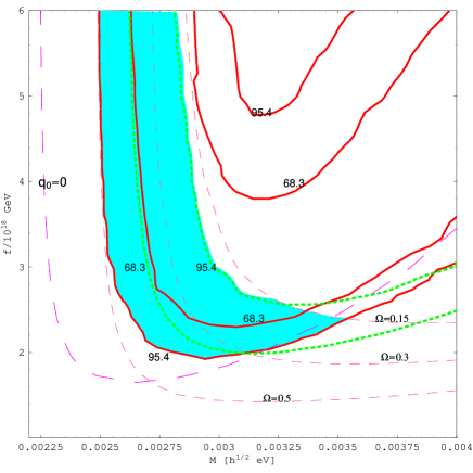
FIG. 1.: Contours of constant likelihood ($95.4\%$ and $68.3\%$) arising from lensing statistics (the region above and to the right of the short dashed curves is excluded) and type Ia supernovae (solid curves) are shown for the PNGB model. Also shown are contours of constant $\Omega_{m0}$ and the limit for present acceleration, $q_{0}=0$. The shaded region shows the parameter space allowed at $95\%$ C.L. by the lensing, SNe, and cluster observations.

For SIS, the total lensing optical depth can be expressed analytically, $\tau(z_{S})=\frac{F}{30}(d_{A}(0,z_{S})(1+z_{S}))^{3}(cH_{0}^{-1})^{-3}$, where $z_{S}$ is the source redshift, $d_{A}(0,z_{S})$ is its angular diameter distance, and $F=16\pi^{3}n(cH_{0}^{-1})^{3}(\sigma_{||}^{*}/c)^{4}\Gamma(1+\alpha+4/\gamma)\simeq 0.026$ measures the effectiveness of the lens in producing multiple images [25]. We correct the optical depth for the effects of magnification bias and include the selection function due to finite angular resolution and dynamic range [29, 30, 8]. We assume a mean optical extinction of $\Delta m$ =$0.5$ mag, as suggested by Falco et al. [31]: this makes the lensing statistics for optically selected quasars consistent with the results for radio sources, for which there is no extinction. When applied to spatially flat cosmological constant models, our approach yields the upper bounds $\Omega_{\Lambda}\lesssim 0.76$ (at $2\sigma$) and $\Omega_{\Lambda}\lesssim 0.61$ (at $1\sigma$), with a best-fit value of $\Omega_{\Lambda}\simeq 0.39$. Recent statistical analyses using both HLQ and radio sources slightly tighten these constraints on a cosmological constant [31]. A combined (optical+radio) lensing analysis for dynamical-$\Lambda$ models is still in progress; qualitatively, we expect this to tighten the lensing constraints below by approximately $1\sigma$.

For the SNe Ia analysis [15], we consider the latest published data from the High-z Supernovae Search Team [1][32]. We use the 27 low-redshift and 10 high-redshift SNe Ia (including SN97ck) reported in Riess et al. [1] and consider data with the MLCS [33, 1] method applied to the supernovae light curves. Following a procedure similar to that described in Riess et al.[1], we determine the cosmological parameters through a $\chi^{2}$ minimization, neglecting the unphysical region $\Omega_{m0}<0$.

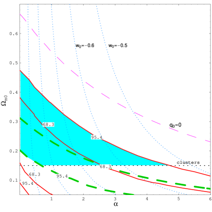
FIG. 2.: Contours of constant likelihood ($95.4\%$ and $68.3\%$) arising from lensing statistics (the region below the thick dashed curves is excluded) and type Ia supernovae (solid curves) are shown for the inverse power-law model. Also shown is the lower bound $\Omega_{m0}=0.15$ from clusters and curves of constant present equation of state $w_{0}=p_{\phi 0}/\rho_{\phi 0}$. The shaded region shows the parameter space allowed at $95\%$ C.L. by the lensing, SNe, and cluster observations.

In Fig. 1 we show the $95.4\%$ and $68.3\%$ C. L. limits from lensing (short dashed contours) and the SNe Ia data (solid curves) on the parameters $f$ and $M$ of the PNGB potential. As in [15], these limits apply to models with the initial condition $\frac{4\sqrt{\pi}\phi(t_{i})}{m_{Pl}}=1.5$ and $\frac{d\phi}{dt}(t_{i})=0$, with $t_{i}=10^{-5}t_{0}$ ; for other choices, the bounding contours would shift by small amounts in the $f-M$ plane. We also plot some contours of constant $\Omega_{m0}$ (dashed) and the curve $q_{0}=0$ (long dashed contour) as a function of the parameters $f$ and $M$. The allowed region (shown by the shaded area in Fig. 1) is limited by the lensing and SNe Ia $95.4\%$ C. L. contours and also by the constraint $\Omega_{m0}>0.15$, which we interpret as $2\sigma$ lower bound from observations of galaxy clusters. The data clearly favors accelerated expansion (the region above the $q_{0}=0$ curve) but curiously there is a small region in the parameter space, close to the point where the $\Omega_{m0}=0.15$ and the Sne Ia $2\sigma$ curves cross, where the Universe is not in accelerated expansion by the present time. This small area disappears if we adopt the tighter constraint $\Omega_{m0}>0.3$. We note that the bulk of the $2\sigma$-allowed parameter space, where the lensing and SNe contours are nearly vertical, corresponds to the scalar field being nearly frozen, i.e., in this region the model is degenerate with a cosmological constant.

In Fig. 2 we show the $95.4\%$ and $68.3\%$ C. L. limits from lensing (thick dashed contours) and the SNe Ia data (solid curves) on the parameters $\alpha$ and $\Omega_{m0}$ of the inverse power-law potential. The horizontal dotted line shows a lower bound on the matter density inferred from the dynamics of galaxy clusters, $\Omega_{m0}=0.15$. We also show contours of the present equation of state $w_{0}=\gamma_{0}-1$ (thin dotted curves) and the curve $q_{0}=0$ (long dashed curve). At $95.4\%$ confidence, the SNe Ia and $\Omega_{m0}$ constraints require $\alpha<5$ and $w_{0}<-0.5$; the latter bound agrees roughly with the constraint obtained by assuming a time-independent equation of state [8], an approximation sometimes used for the inverse power-law model. We also observe that the lensing constraints on the model parameters are weak, constraining only low values of $\Omega_{m0}$ and $\alpha$. We remark, however, that they are consistent with the SNe Ia constraints. We can tighten the constraints on the equation of state if we consider a higher value for the $\Omega_{m0}$ lower bound. For instance, if we adopt $\Omega_{m0}>0.3$, as suggested in [34], we obtain $w_{0}<-0.67$ and $\alpha<1.8$. In both models, a larger lower bound on $\Omega_{m0}$ pushes the scalar field behavior toward that of the cosmological constant ($w=-1$).

IV Conclusion

A consensus is beginning to emerge that we live in a nearly flat, low-matter-density Universe with $\Omega_{m0}\sim 0.3$ and a dark energy, negative-pressure component with $\Omega_{X}\sim 0.7$. The nature of this dark energy component is still not well understood; further developments will require deeper understanding of fundamental physics as well as improved observational tests to measure the equation of state at recent epochs, $w(t)$, and determine if it is distinguishable from that of the cosmological constant [35]. Classical scalar field models provide a simple dynamical framework for posing these questions. In this paper we analyzed two representative scalar field models, the PNGB and power-law potentials, which span the range of expected dynamical behavior. The inverse power-law model displays tracking solutions [21] which allow the scalar field to start from a wide set of initial conditions. We showed that current data favors a small value of the parameter, $\alpha<5$. This may be a problem for these models: in Refs:[21] it was shown that, starting from the equipartition condition after inflation, it is necessary to have $\alpha>5$ for the field to begin tracking before matter-radiation equality. Since the observational constraints indicate that tracking could only be achieved (if at all) at more recent times, it is not clear what theoretical advantage, in terms of alleviating the ‘cosmic coincidence’ problem, is gained by the tracking solution. Although well motivated from the particle physics viewpoint, the PNGB model is strongly constrained by the SNe Ia and lensing data. Finally, as noted above, these two models predict radically different futures for the Universe. In the inverse power law model, the expansion will continue accelerating and approach de Sitter space. In the PNGB model, the present epoch of acceleration may be brief, followed by a return to what is effectively matter-dominated evolution.

- [1] A. G. Riess et al.,Astron. J. 116 , 1009 (1998); P. M. Garnavich et al., Astrophys. J. 509, 74 (1998).
- [2] S. Perlmutter et al., Astrophys. J. 517, 565, (1999).
- [3] S. Dodelson and L. Knox, astro-ph/9909454.
- [4] A. Melchiorri et al., astro-ph/9911445.
- [5] N. A. Bahcall, J. P. Ostriker, S. Perlmutter and P. J. Steinhardt Science, 284, 1481 (1999); M. S. Turner, astro-ph/9901109.
- [6] P.J.E. Peebles, Astrophys. J. 284, 439 (1984); M. S. Turner, G.Steigman, L. M. Krauss, Phys. Rev. Lett. 52, 2090 (1984).
- [7] B. Ratra and A. Quillen, Mon. Not. R. Astron. Soc., 259, 738, (1992); L. F. Bloomfield Torres and I. Waga, Mon. Not. R. Astron. Soc. 279, 712 (1996); A. R. Cooray, Astron. Astrophys. 342, 353 (1999).
- [8] I. Waga and A. P. M. R. Miceli, Phys. Rev. D 59, 103507, (1999).
- [9] Y. B. Zeldovich, Sov. Phys. Uspekhi 11 , 381 (1968).
- [10] S. Weinberg, Rev. Mod. Phys. 61, 1 (1989); S. M. Carroll, W. H. Press and E. L. Turner, Annu. Rev. Astron. Astrophys.,30, 499 (1992); J. Frieman, in “Third Paris Cosmology Colloquium”, eds. H. J. de Vega & N. Sanchez (World Scientific, 1995); V. Sahni and A. Starobinsky, astro-ph/9904398.
- [11] J. A. Frieman, C. T. Hill, and R. Watkins, Phys. Rev. D 46, 1226 (1992).
- [12] J. A. Frieman, C. T. Hill, A. Stebbins and I. Waga, Phys. Rev. Lett. 75, 2077 (1995).
- [13] M. Fukugita and T. Yanagida, preprint YITP/K-1098 (1995).
- [14] K. Coble, S. Dodelson, and J. A. Frieman, Phys. Rev. D 55, 1851 (1997).
- [15] J. A. Frieman and I. Waga, Phys. Rev. D 57, 4642 (1998).
- [16] R. R. Caldwell, R. Dave, and P.J. Steinhardt, Phys. Rev. Lett. 80, 1582 (1998).
- [17] B. Ratra and P. J. E. Peebles, Phys. Rev. D 37, 3407 (1988); P. J. E. Peebles and B. Ratra, Astrophys. J. 325, L17 (1988).
- [18] M. Ozer and M. O. Taha, Nucl. Phys. B287, 776 (1987); K. Freese et al., Nucl. Phys. B287, 797 (1987); M. Reuter and C. Wetterich, Phys. Lett. B188, 38 (1987); W. Chen and Y. S. Wu, Phys. Rev. D 41, 695 (1990); J. C. Carvalho, J. A. S. Lima and I. Waga, Phys. Rev. D 46, 2404, (1992); I. Waga, Astrophys. J. 414, 436 (1993); V. Silveira and I. Waga, Phys. Rev. D 50, 4890 (1994); V. Silveira and I. Waga, Phys. Rev. D 56, 4625 (1997); J. M. Overduin and F. I. Cooperstock, Phys. Rev. D 58, 043506, (1998).
- [19] A. Vilenkin, Phys. Rev. Lett., 53, 1016 (1984); J. N. Fry, Phys. Lett. B158, 211 (1985); H. A. Feldman and A. E. Evrard, Int. J. Mod. Phys. D2, 113 (1993); J. Stelmach and M. P. Dabrowski, Nucl. Phys. B406, 471 (1993); H. Martel, Astrophys. J. 445, 537 (1995); L. M. A. Bittencourt, P. Laguna, R. A. Matzner, hep-ph/9612350; M. Kamionkowski and N. Toumbas, Phys. Rev. Lett., 77, 587 (1997); D. N. Spergel and U. L. Pen, Astrophys. J. 491, L67 (1997); T. Chiba, N. Sugiyama, and T. Nakamura, Mon. Not. R. Astron. Soc. 289, 5 (1997); M. S. Turner and M. White, Phys. Rev. D 56, R4439 (1997); M. White, Astrophys. J. 506, 485 (1998); W. Hu, Astrophys. J. 506, 495 (1998); S. Perlmutter, M.S. Turner and M. White, Phys. Rev. Lett. 83, 670 (1999); M. Bucher and D. Spergel, Phys. Rev. D 60, 043505, (1999); L. Wang, R. R. Caldwell, J. P. Ostriker and P. J. Steinhardt, astro-ph/9901388.
- [20] C. Wetterich, Nuclear Physics B302, 668 (1988); V. Sahni, H. A. Feldman and A. Stebbins, Astrophys. J. 385, 1 (1992); P. T. P. Viana and A. R. Liddle, Phys. Rev. D 57, 674 (1998); P. Ferreira and M. Joyce, Phys. Rev. Lett., 79, 4740 (1997); Phys. Rev. D 58, 023503 (1998); A. Liddle and R. Scherrer, Phys. Rev D 59, 023509 (1999); J. Uzan, Phys. Rev D 59, 123510 (1999); P. Binétruy, Phys. Rev D 60, 063502 (1999); A. Masiero, M. Pietroni and F. Rosati, hep-ph/9905346; L. Amendola, astro-ph/9906073 ; astro-ph/9908023; A. Albrecht and C. Skordis, astro-ph/9908085; V. Sahni and L. Wang , astro-ph/9910097;
- [21] I. Zlatev, L. Wang and P. J. Steinhardt, Phys. Rev. Lett. 82, 896 (1999); P. J. Steinhardt, L. Wang and I. Zlatev, Phys. Rev D 59, 123504 (1999).
- [22] S. M. Carroll, Phys. Rev. Lett 81, 3067 (1998); C. Kolda and D. H. Lyth, Phys. Lett B458, 197 (1999); K. Choi, hep-ph/9912218.
- [23] S. Podariu and B. Ratra, astro-ph/9910527.
- [24] D. Maoz et al., Astrophys. J. 409, 28 (1993); D. Crampton ,R. D. McClure, and J. M. Fletcher, ibid. 392, 23 (1992); H. K. C. Yee , A. V. Filipenko, and D. H. Tang, A. J. 105, 7 (1993); J. Surdej et al., ibid. 105, 2064 (1993); E. E. Falco, in Gravitational Lenses in the Universe, edited by J. Surdej, D. Fraipont-Caro, E. Gosset, S. Refsdal, and M. Remy (Liege: Univ. Liege), p. 127 (1994); C. S. Kochanek, E. E. Falco, and R. Shild, Astrophys. J. 452, 109 (1995); A. O. Jaunsen et al., Astron. Astrophys. 300, 323 (1995).
- [25] E. L. Turner, J. P. Ostriker, J. R. Gott III, Astrophys. J. 284, 1, (1984).
- [26] S. M. Faber and R. E. Jackson, Astrophys. J. 204, 668 (1976).
- [27] P. Schechter, Astrophys. J. 203, 297 (1976).
- [28] J. Loveday, B. A. Peterson, G. Efstathiou and S. J. Maddox, Astrophys. J. 390, 338 (1994).
- [29] C. S. Kochanek, Astrophys. J. 419, 12 (1993).
- [30] C. S. Kochanek, Astrophys. J. 466, 47 (1996).
- [31] E. E. Falco, C. S. Kochanek and J. A. Muñoz, Astrophys. J. 494, 47 (1998).
- [32] The results would not change appreciably if we had considered data from [2].
- [33] A. G. Riess, W. H. Press and R. P. Kirchner, Astrophys. J. 473, 88 (1996).
- [34] I. Zehavi and A. Dekel, Nature 401, 252 (1999).
- [35] A. R. Cooray and D. Huterer, Astrophys. J. 513, L95 (1999); D. Huterer and M. S. Turner, Phys. Rev. D 60, 081301 (1999); T. D. Saini, S. Raychaudhury, V. Sahni and A. A. Starobinsky, astro-ph/9910231.