Probing The Gravity Induced Bias with Weak Lensing:
Test of Analytical results Against Simulations

Abstract

Future weak lensing surveys will directly probe the density fluctuation in the universe. Recent studies have shown how the statistics of the weak lensing convergence field is related to the statistics of collapsed objects. Extending earlier analytical results on the probability distribution function of the convergence field we show that the bias associated with the convergence field can directly be related to the bias associated with the statistics of underlying over-dense objects. This will provide us a direct method to study the gravity induced bias in galaxy clustering. Based on our analytical results which use the hierarchical ansatz for non-linear clustering, we study how such a bias depends on the smoothing angle and the source red-shift. We compare our analytical results against ray tracing experiments through N-body simulations of four different realistic cosmological scenarios and found a very good match. Our study shows that the bias in the convergence map strongly depends on the background geometry and hence can help us in distinguishing different cosmological models in addition to improving our understanding of the gravity induced bias in galaxy clustering.

1 Introduction

Weak gravitational lensing (Bartelmann & Schneider 1999) is the distortion of images of the background galaxies through the tidal gravitational field of large scale background mass distribution. Study of such distortions provides us an unique way to probe statistical properties of intervening mass distribution.

Although there is no generally applicable definition of weak lensing the common aspect of all studies in weak gravitational lensing is that measurements of its effects are statistical in nature. Pioneering works in this direction were done by Blandford et al. (1991), Miralda-Escude (1991) and Kaiser (1992) based on the earlier work by Gunn (1967). Current progress in weak lensing can broadly be divided into two distinct categories. Where as Villumsen (1996), Stebbins (1996), Bernardeau et al. (1997) and Kaiser (1987) have focussed on linear and quasi-linear regime by assuming a large smoothing angle, several authors have developed a numerical technique to simulate weak lensing catalogs. Numerical simulations of weak lensing typically employ N-body simulations, through which ray tracing experiments are conducted (Schneider & Weiss 1988; Jarosszn’ski et al. 1990; Lee & Paczyn’ski 1990; Jarosszn’ski 1991; Babul & Lee 1991; Bartelmann & Schneider 1991, Blandford et al. 1991). Building on the earlier work of Wambsganns et al. (1995, 1997, 1998) most detailed numerical study of lensing was done by Wambsganns, Cen & Ostriker (1998). Other recent studies using ray tracing experiments have been conducted by Premadi, Martel & Matzner (1998), van Waerbeke, Bernardeau & Mellier (1998), Bartelmann et al (1998) and Couchman, Barber & Thomas (1998). While peturbative analysis can provide valuable information at large smoothing angle such analysis can not be used to study lensing at small angular scales as the whole perturbative series starts to diverge.

A complete analysis of the weak lensing statistics at small angular scales will require a similar analysis for the underlying dark matter distribution which we do not have at present. However there are several non-linear ansatze which predict a tree hierarchy for matter correlation functions and are thought to be successful to some degree in modeling results from numerical simulations. Most of these ansatze assumes a tree hierarchy for higher order correlation functions and they disagree with each other by the way they assign weights to trees of same order but of different topologies (Balian & Schaeffer 1989, Bernardeau & Schaeffer 1992; Szapudi & Szalay 1993). Evolution of two-point correlation functions in all such approximations are left arbitrary. However recent studies by several authors (Hamilton et al 1991; Nityananda & Padmanabhan 1994; Padmanabhan et al. 1996; Jain, Mo & White 1995; Peacock & Dodds 1996) have provided us a very accurate fitting formula for the evolution of the two-point correlation function which can be used in combination with these hierarchical ansatze to predict clustering properties of dark matter distribution in the universe.

Most recent studies in weak lensing have mainly focussed on lower order cumulants (van Waerbeke, Bernardeau & Mellier 1998, Hui 1999, Munshi & Jain 1999a), cumulant correlators (Munshi & Jain 1999b) and errors associated with their measurement from observational data using different filter functions (Reblinsky et al. 1999). However it is well known that higher order moments and more sensitive to the tail of the distribution function which they represent and are sensitive to measurement errors due to finite size of catalogs (Szapudi & Colombi 1996). On the other hand numerical simulations involving ray tracing techniques have already shown that while probability distribution function (PDF) associated with density field is not sensitive to cosmological parameters its weak lensing counterpart can lift such a degeneracy and can help us in estimation of cosmological parameters from observational data (Jain, Seljak & White 1999). Munshi & Jain (1999a,b) extended such studies to show that the hierarchical ansatz can actually be used to make concrete analytical predictions for lower order statistical properties of the convergence field. Valageas (1999a) has used hierarchical ansatz for computing error involved in estimation of $\Omega_{0}$ and $\Lambda$ from SNeIa observations. A similar fitting function was recently proposed by Wang (1999). Our formalism is similar to that of Valageas (1999a) although the results obtained by us include the effect of smoothing and analysis presented here correspond to the joint probability distribution function of two smoothed patches and hence the bias associated with them. Our formalism presented here is an extension of the study of the PDF using similar techniques (Munshi & Jain 1999b, Valageas 1999b), it can very easily be extended to multi-point PDF and hence to compute the $S_{N}$ parameters associated with “hot spots” of the convergence maps. Analytical results and detailed comparison against numerical simulations will be presented elsewhere (Munshi & Coles 1999a,b).

The paper is organized as follows. In section $2$ we describe briefly ray tracing simulations. Section $3$ presents most of the analytical results necessary for computation of the bias of the smoothed convergence field $\kappa_{s}$. Results of data analysis are presented in section $4$. Section $5$ is left for discussion of our result in general cosmological framework.

2 Generation of Convergence Maps from N-body Simulations

Convergence maps are generated by solving the geodesic equations for the propagation of light rays through N-body simulations of dark matter clustering. The simulations used for our study are adaptive $P^{3}M$ simulations with $256^{3}$ particles and were carried out using codes kindly made available by the VIRGO consortium. These simulations can resolve structures larger than $30h^{-1}kpc$ at $z=0$ accurately. These simulations were carried out using 128 or 256 processors on CRAY T3D machines at Edinburgh Parallel Computer Center and at the Garching Computer Center of the Max-Planck Society. These simulations were intended primarily for studies of the formation and clustering of galaxies (Kauffmann et al 1999a, 1999b; Diaferio et al 1999) but were made available by these authors and by the Virgo Consortium for this and earlier studies of gravitational lensing (Jain, Seljak & White 1999, Reblinsky et al. 1999, Munshi & Jain 1999a,b).

Ray tracing simulations were carried out by Jain et al. (1999) using a multiple lens-plane calculation which implements the discrete version of recursion relations for mapping the photon position and the Jacobian matrix (Schneider & Weiss 1988; Schneider, Ehler & Falco 1992). In a typical experiment $4\times 10^{6}$ rays are used to trace the underlying mass distribution. The dark matter distribution between the source and the observer is projected onto $20$ - $30$ planes. The particle positions on each plane are interpolated onto a $2048^{2}$ grid. On each plane the shear matrix is computed on this grid from the projected density by using Fourier space relations between the two. The photons are propagated starting from a rectangular grid on the first lens plane. The regular grid of photon position gets distorted along the line of sight. To ensure that all photons reach the observer, the ray tracing experiments are generally done backward in time from the observer to the source plane at red-shift $z=z_{s}$. The resolution of the convergence maps is limited by both the resolution scale associated with numerical simulations and also due to the finite resolution of the grid to propagate photons. The outcome of these simulations are shear and convergence maps on a two dimensional grid. Depending on the background cosmology the two dimensional box represents a few degree scale patch on the sky. For more details on the generation of $\kappa$-maps, see Jain et al (1999).

3 Analytical Predictions

In this section we will provide necessary theoretical background for the bias function in the context of hierarchical clustering.

We will be using the following line element for the background geometry of the universe:

$$d\tau^{2}=-c^{2}dt^{2}+a^{2}(t)(d\chi^{2}+r^{2}(\chi)d^{2}\Omega)$$ (1)

Where we have denoted angular diameter distance by $r(\chi)$ and scale factor of the universe by $a(t)$. $r(\chi)=K^{-1/2}\sin(K^{-1/2}\chi)$ for positive curvature, $r(\chi)=(-K)^{-1/2}\sinh((-K)^{-1/2}\chi)$ for negative curvature and $\chi$ for the flat universe. For a present value of of $H_{0}$ and $\Omega_{0}$ we have $K=(\Omega_{0}-1)H_{0}^{2}$. The various parameters charecterising different cosmological models are listed in Table - 1.

Table 1: Cosmological Parameters charecterising different models

	SCDM	TCDM	LCDM	OCDM
$\Gamma$	0.5	0.21	0.21	0.21
$\Omega_{0}$	1.0	1.0	0.3	0.3
$\Lambda_{0}$	0.0	0.0	0.7	0.0
$\sigma_{8}$	0.6	0.6	0.9	0.85
$H_{0}$	50	50	70	70

3.1 The Formalism

The statistics of weak lensing convergence $\kappa$ is very much similar to that of the projected density field. In what follows we will be considering a small patch of the sky where we can use the plane parallel approximation or small angle approximation to replace spherical harmonics by Fourier modes. The 3D density contrast $\delta$ along the line of sight when projected into 2D sky with a weight function $\omega(\chi)$ will provide us the projected density contrast or the weak-lensing convergence at a direction $\gamma$.

$$\kappa({\bf\gamma}_{1})={\int_{0}^{\chi_{s}}}{d\chi}_{1}\omega(\chi_{1})\delta(r(\chi){\bf\gamma}_{1})$$ (2)

In all our discussion we will be placing the sources at a fixed red-shift (an approximation not too difficult to modify for more realistic description), the weight function can be expressed as $\omega(\chi)=3/4ac^{-2}H_{0}^{2}\Omega_{m}r(\chi)r(\chi_{s}-\chi)/r(\chi_{s})$. Where $\chi_{s}$ is the comoving radial distance to the source at a redshift $z_{s}$. Fourier decomposition of $\delta$ can be written as:

$$\kappa(\gamma_{1})={\int_{0}^{\chi_{s}}}{d\chi}_{1}\omega(\chi_{1})\int{d^{3}{\bf k}\over{(2\pi)}^{3}}\exp(i\chi_{1}k_{\parallel}+ir\theta k_{\perp})\delta_{k}$$ (3)

Where we have used $k_{\parallel}$ and $k_{\perp}$ to denote components of wave vector ${\bf k}$ parallel and perpendicular to line of sight direction $\gamma$. In small angle approximation however one assumes that $k_{\perp}$ much larger compared to $k_{\parallel}$. We will denote the angle between the line of sight direction ${\bf\gamma}$ and the wave vector ${\bf k}$ by $\theta$. Using the definitions we have introduced above we can compute the smoothed projected two-point correlation function (Peebles 1980, Kaiser 1992, Kaiser 1998):

$$\langle\kappa(\gamma_{1})\kappa(\gamma_{2})\rangle_{c}={\int_{0}^{\chi_{s}}}d{\chi_{1}}{\omega^{2}(\chi_{1})\over r^{2}(\chi_{1})}\int{d^{2}{\bf l}\over(2\pi)^{2}}~{}\exp(\theta l)~{}{\rm P}{\big{(}{l\over r(\chi)}\big{)}}W_{2}^{2}(l\theta_{0}).$$ (4)

Where we have introduced a new notation ${\bf l}=r(\chi){\bf k}_{\perp}$ which denotes a scaled wave vector projected on the surface of the sky. The average of two-point correlation function $\langle\kappa_{s}^{2}\rangle$ smoothed over an angle $\theta_{0}$ with a top-hat smoothing window $W_{2}(l\theta_{0})$ is useful to quantify the fluctuations in $\kappa_{s}$ which is often used to reconstruct the matter power spectrum $P({\bf k})$ (Jain, Selzak & White 1998).

$$\langle\kappa_{s}^{2}\rangle_{c}={\int_{0}^{\chi_{s}}}d{\chi_{1}}{\omega^{2}(\chi_{1})\over r^{2}(\chi_{1})}\int{d^{2}{\bf l}\over(2\pi)^{2}}~{}{\rm P}{\big{(}{l\over r(\chi)}\big{)}}W_{2}^{2}(l\theta_{0})$$ (5)

Similar analysis for the higher order cumulant correlators (Szapudi & Szalay 1997, Munshi & Coles 1999) of the smoothed convergence field relating $\langle\kappa_{s}^{m}(\gamma_{1})\kappa_{s}^{n}(\gamma_{2})\rangle_{c}$ with multi-spectra of underlying dark matter distribution $B_{p}$ (Munshi & Coles 1999a):

$$\langle\kappa_{s}^{2}(\gamma_{1})\kappa_{s}(\gamma_{2})\rangle_{c}=\int_{0}^{\chi_{s}}{\omega^{3}(\chi)\over r^{4}(\chi)}d\chi\int\frac{d^{2}{\bf l}_{1}}{(2\pi)^{2}}\int\frac{d^{2}{\bf l}_{2}}{(2\pi)^{2}}W_{2}(l_{1}\theta_{0})W_{2}(l_{2}\theta_{0})W_{2}(l_{3}\theta_{0})\exp(il_{2}\theta_{12})B_{3}\left({{\bf l}_{1}\over r(\chi)},{{\bf l}_{2}\over r(\chi)},{{\bf l}_{3}\over r(\chi)}\right);$$ (6)

$$\langle\kappa_{s}^{3}(\gamma_{1})\kappa_{s}(\gamma_{2})\rangle_{c}=\int_{0}^{\chi_{s}}{\omega^{3}(\chi)\over r^{4}(\chi)}d\chi\int\frac{d^{2}{\bf l}_{1}}{(2\pi)^{2}}\int\frac{d^{2}{\bf l}_{2}}{(2\pi)^{2}}\int\frac{d^{2}{\bf l}_{3}}{(2\pi)^{2}}W_{2}(l_{1}\theta_{0})W_{2}(l_{2}\theta_{0})W_{2}(l_{3}\theta_{0})W_{2}(l_{4}\theta_{0})\exp(il_{3}\theta_{12})$$

$$B_{4}\left({{\bf l}_{1}\over r(\chi)},{{\bf l}_{2}\over r(\chi)},{{\bf l}_{3}\over r(\chi)},{{\bf l}_{4}\over r(\chi)}\right);$$ (7)

$$\langle\kappa_{s}^{2}(\gamma_{1})\kappa_{s}^{2}(\gamma_{2})\rangle_{c}=\int_{0}^{\chi_{s}}{\omega^{3}(\chi)\over r^{4}(\chi)}d\chi\int\frac{d^{2}{\bf l}_{1}}{(2\pi)^{2}}\int\frac{d^{2}{\bf l}_{2}}{(2\pi)^{2}}\int\frac{d^{2}{\bf l}_{3}}{(2\pi)^{2}}W(l_{1}\theta_{0})W_{2}(l_{2}\theta_{0})W_{2}(l_{3}\theta_{0})W_{2}(l_{4}\theta_{0})\exp(i(l_{1}+l_{2})\theta_{12})$$

$$B_{4}\left({{\bf l}_{1}\over r(\chi)},{{\bf l}_{2}\over r(\chi)},{{\bf l}_{3}\over r(\chi)},{{\bf l}_{4}\over r(\chi)}\right).$$ (8)

In general we can express the cumulant correlators of arbitrary order $\langle\kappa_{s}^{m}(\gamma_{1})\kappa_{s}^{n}(\gamma_{2})\rangle_{c}$ in terms of multi-spectra $B_{m+n}$ as:

$$\langle\kappa_{s}^{m}(\gamma_{1})\kappa_{s}^{n}(\gamma_{2})\rangle_{c}=\int_{0}^{\chi_{s}}{\omega^{n+m}(\chi)\over r^{2(n+m-1)}(\chi)}d\chi\int\frac{d^{2}{\bf l}_{1}}{(2\pi)^{2}}\dots\int\frac{d^{2}{\bf l}_{n+m-1}}{(2\pi)^{2}}W_{2}(l_{1}\theta_{0})\dots W_{2}(l_{n+m}\theta_{0})\exp[i(l_{1}+\dots+l_{m})\theta_{12}]$$

$$B_{m+n}\left({{\bf l}_{1}\over r(\chi)},\dots,{{\bf l}_{m+n}\over r(\chi)}\right).$$ (9)

We will use and extend these results in this paper to show that it is possible to compute the whole bias function $b(>\kappa_{s})$, i.e. the bias associated with those spots in convergence map which $\kappa_{s}$ is above certain threshold (which acts as a generating function for these cumulant correlators) from the statistics of underlying over-dense dark objects.Details of analytical results presented here can be found in Munshi & Coles (1999b).

3.2 Hierarchical Ansatze

In deriving the above expressions we have not used any specific form for the matter correlation hierarchy, however the length scales involved in small angles are in the highly non-linear regime. Assuming a tree model for the matter correlation hierarchy in the highly non-linear regime one can write the most general case as (Groth & Peebles 1977; Fry & Peebles 1978; Davis & Peebles 1983; Bernardeau & Schaeffer 1992; Szapudi & Szalay 1993):

$$\xi_{N}({\bf r_{1}},\dots{\bf r_{N}})=\sum_{\alpha,\rm N-trees}Q_{N,\alpha}\sum_{\rm labellings}\prod_{\rm edges(i,j)}^{(N-1)}\xi({\bf r_{i}},{\bf r_{j}})$$ (10)

It is interesting to note that an exactly similar hierarchy develops in the quasi-linear regime in the limit of vanishing variance (Bernardeau 1992), however the hierarchal amplitudes $Q_{N,\alpha}$ become shape dependent in such a case. In the highly nonlinear regime there are some indications that these functions become independent of shape parameters as has been proved by studies of lowest order parameter $Q_{3}=Q$ using high resolution numerical simulations (Sccociamarro et al. 1998). In the Fourier space such an ansatz will mean that the whole hierarchy of multi-spectra $B_{p}$ can be written in terms of sum of products of power-spectra, e.g. in low orders we can write:

$$B_{2}({\bf k}_{1},{\bf k}_{2},{\bf k}_{3})_{\sum k_{i}=0}=Q(P({\bf k_{1}})P({\bf k_{2}})+P({\bf k_{2}})P({\bf k_{3}})+P({\bf k_{3}})P({\bf k_{1}})),$$ (11)

$$B_{3}({\bf k}_{1},{\bf k}_{2},{\bf k}_{3},{\bf k}_{4})_{\sum k_{i}=0}=R_{a}P({\bf k_{1}})P({\bf k_{1}+k_{2}})P({\bf k_{1}+k_{2}+k_{3}})+{\rm cyc.perm.}+R_{b}P({\bf k_{1}})P({\bf k_{2}})p({\bf k_{3}})+{\rm cyc.perm.}$$ (12)

Different hierarchal models differ the way they predict the amplitudes of different tree topologies. Bernardeau & Schaeffer (1992) considered the case where amplitudes in general are factorizable, at each order one has a new “star” amplitude and higher order “snake” and “hybrid” amplitudes are constructed from lower order “star” amplitudes (see Munshi, Melott & Coles 1999a,b,c for a detailed description). In models proposed by Szapudi & Szalay (1993) it is assumed that all hierarchal amplitudes of a given order are actually degenerate.

We do not use any of these specific models for clustering and only assume a hierarchal nature for the higher order correlation functions. Galaxy surveys have been used to study these ansatze. Our main motivation here is to show that weak-lensing surveys can also provide valuable information in this direction, in addition to constraining matter power-spectra and the background geometry of the universe. The most general form for the lower order cumulant correlators in the large separation limit can be expressed as:

$$\langle\kappa_{s}^{2}(\gamma_{1})\kappa_{s}(\gamma_{2})\rangle_{c} = 2Q_{3}{\cal C}_{3}[\kappa_{\theta_{0}}\kappa_{\theta_{12}}]=C_{21}^{\eta}{\cal C}_{3}[\kappa_{\theta_{0}}\kappa_{\theta_{12}}]\equiv C_{21}^{\kappa}\langle\kappa_{s}^{2}\rangle_{c}\langle\kappa_{s}(\gamma_{1})\kappa_{s}(\gamma_{2})\rangle_{c},$$ (13)

$$\langle\kappa_{s}^{3}(\gamma_{1})\kappa_{s}(\gamma_{2})\rangle_{c} = (3R_{a}+6R_{b}){\cal C}_{4}[\kappa_{\theta_{0}}^{2}\kappa_{\theta_{12}}]=C_{31}^{\eta}{\cal C}_{4}[\kappa_{\theta_{0}}^{2}\kappa_{\theta_{12}}]\equiv C_{31}^{\kappa}\langle\kappa_{s}^{2}\rangle_{c}^{2}\langle\kappa_{s}(\gamma_{1})\kappa_{s}(\gamma_{2})\rangle_{c},$$ (14)

$$\langle\kappa_{s}^{2}(\gamma_{1})\kappa_{s}^{2}(\gamma_{2})\rangle_{c} = 4R_{b}{\cal C}_{4}[\kappa_{\theta_{0}}^{2}\kappa_{\theta_{12}}]=C_{22}^{\eta}{\cal C}_{4}[\kappa_{\theta_{0}}\kappa_{\theta_{12}}]\equiv C_{22}^{\kappa}\langle\kappa_{s}^{2}\rangle_{c}^{2}\langle\kappa_{s}(\gamma_{1})\kappa_{s}(\gamma_{2})\rangle_{c},$$ (15)

$$\langle\kappa_{s}^{4}(\gamma_{1})\kappa_{s}(\gamma_{2})\rangle_{c} = (24S_{a}+36S_{b}+4S_{c}){\cal C}_{5}[\kappa_{\theta_{0}}^{3}\kappa_{\theta_{12}}]=C_{41}^{\eta}{\cal C}_{5}[\kappa_{\theta_{0}}^{3}\kappa_{\theta_{12}}]\equiv C_{41}^{\kappa}\langle\kappa_{s}^{2}\rangle_{c}^{3}\langle\kappa_{s}(\gamma_{1})\kappa_{s}(\gamma_{2})\rangle_{c},$$ (16)

$$\langle\kappa_{s}^{3}(\gamma_{1})\kappa_{s}^{2}(\gamma_{2})\rangle_{c} = (12S_{a}+6S_{b}){\cal C}_{5}[\kappa_{\theta_{0}}^{3}\kappa_{\theta_{12}}]=C_{32}^{\eta}{\cal C}_{5}[\kappa_{\theta_{0}}^{3}\kappa_{\theta_{12}}]\equiv C_{32}^{\kappa}\langle\kappa_{s}^{2}\rangle_{c}^{3}\langle\kappa_{s}(\gamma_{1})\kappa_{s}(\gamma_{2})\rangle_{c}.$$ (17)

Where $C_{mn}^{\kappa}$ denotes the cumulant correlators of the convergence field and $C_{mn}^{\eta}$ denotes the cumulant correlators for the underlying mass distribution. Extending above results to arbitrary order we can write:

$$\langle\kappa_{s}^{p}(\gamma_{1})\kappa_{s}^{q}(\gamma_{2})\rangle_{c}=C_{pq}^{\eta}{\cal C}_{p+q}[\kappa_{\theta_{0}}^{(p+q-2)}\kappa_{\theta_{12}}]=C_{pq}^{\kappa}\langle\kappa_{s}^{2}\rangle_{c}^{(p+q-2)}\langle\kappa_{s}(\gamma_{1})\kappa_{s}(\gamma_{2})\rangle_{c}.$$ (18)

where $C_{pq}^{\eta}$ denotes the cumulant correlators for the underlying mass distribution,

$${\cal C}_{t}[\kappa^{m}_{\theta_{0}}\kappa_{\theta_{12}}]=\int_{0}^{\chi_{s}}{\omega^{t}(\chi)\over r^{2(t-1)}(\chi)}\kappa^{m}_{\theta_{0}}\kappa_{\theta_{12}}d\chi,$$ (19)

similarly the following notations were used to simplify the above expressions:

$$\kappa_{\theta_{0}} \equiv \int\frac{d^{2}\bf l}{(2\pi)^{2}}P\left({l\over r(\chi)}\right)W_{2}^{2}(l\theta_{0}),$$ (20)

$$\kappa_{\theta_{12}} \equiv \int\frac{d^{2}\bf l}{(2\pi)^{2}}P\left({l\over r(\chi)}\right)W_{2}^{2}(l\theta_{0})\exp(l\theta_{12}).$$ (21)

.

The hierarchical expression for the lowest order cumulant i.e. $S_{3}$ was derived by Hui 1998. He also showed that his result agrees well with numerical ray tracing experiments by Jain, Seljak and White (1998). More recent studies have shown that higher order cumulants and even the two-point statistics such as cumulant correlators can also be reliably modeled in a similar way (Munshi & Coles 1999, Munshi & Jain 1999a). We extend such results in this paper to compute the complete bias function $b_{\kappa}(\kappa_{s})$ (which is related to the low order two-point statistics such as the cumulant correlators defined above) associated with high $\kappa_{s}$ spots in the convergence map,

$$p_{\kappa}(\kappa_{1},\kappa_{2})d\kappa_{1}d\kappa_{2}=p_{\kappa}(\kappa_{1})p_{\kappa}(\kappa_{2})(1+b_{\kappa}(\kappa_{1})\xi^{\kappa}_{12}b_{\kappa}(\kappa_{2}))d\kappa_{1}d\kappa_{2},$$ (22)

and its relation to the bias associated with collapsed objects in underlying density field $1+\delta$.

3.3 The bias associated with collapsed objects

The success of analytical results in predicting the lower order cumulants, cumulant correlators and the one-point smoothed PDF(Munshi & Coles 199a,b; Munshi & Jain 1999a,b; Valageas 1999a,b), motivates a general analysis of the bias associated with the high $\kappa_{s}$ spots in convergence maps and their relation with bias associated with the high peaks in the underlying mass distribution. For this purpose we found that formalism developed by Balian & Schaeffer (1989) and Bernardeau & Schaeffer (1992) (later extended Bernardeau (1992, 1994)) to be most suitable. These results are based on a very general tree hierarchy for higher order correlation function and the assumption that amplitudes associated with different tree-topologies are constant once in the highly non-linear regime. Later these results were generalized by Bernardeau (1992, 1994) for the case of quasi-linear regime too, where perturbative dynamics can be used to make more concrete predictions. Errors associated with top-hat smoothing and its use with hierarchical ansatz has been studied in detail by Szapudi et al.(1992) and Boschan et al. (1994) and will be assumed small even in the case of two-point cumulant correlators throughout this paper. In this section we review the basic results from scaling models in the highly non-linear regime and quasi-linear regime before extending such models to the statistics of smoothed convergence field $\kappa(\theta_{0})$ where we will show that although weak lensing statistics probes the highly non-linear regime, projection effects make the variance smaller than unity justifying the use of quasi-linear results even though the generating function remains the one for highly non-linear regime. We will be using the small angle approximation in our derivation. Our results can in principle be generalized for the case of projected galaxy catalogs too, a detailed analysis will be presented elsewhere.

3.3.1 The Generating Function

In scaling analysis of the probability distribution function (PDF) the void probability distribution function (VPF) plays most fundamental role, which can related to the generating function of the cumulants or $S_{N}$ parameters, $\phi(y)$ (White 1979, Balian & Schaeffer 1989)

$$P_{v}(0)=\exp(-\bar{N}\sigma(N_{c}))=\exp\Big{(}-{\phi(N_{c})\over\bar{\xi}_{2}}\Big{)}.$$ (23)

Where $P_{v}(0)$ is the probability of having no “particles” in a cell of of volume $v$, $\bar{N}$ is the average occupancy of these “particles” and $N_{c}=\bar{N}{\bar{\xi}}_{2}$. The VPF is meaningful only for discrete distribution of particles and can not be defined for smooth density fields such as $\delta$ or $\kappa(\theta_{0})$. However the scaling functions defined above $\sigma(y)=-{\phi(y)\over y}$ are very much useful even for continuous distributions where they can be used as a generating function of one-point cumulants or $S_{p}$ parameters,

$$\phi(y)=\sum_{p=1}^{\infty}{S_{p}\over p!}y^{p}.$$ (24)

The function $\phi(y)$ satisfies the constraint $S_{1}=S_{2}=1$ necessary for proper normalization of PDF. The other generating function which plays a very important role in such analysis is the generating function for vertex amplitudes $\nu_{n}$, associated with nodes appearing in tree representation of higher order correlation hierarchy ($Q_{3}=\nu_{2}$, $R_{a}=\nu_{2}^{2}$ and $R_{b}=\nu_{3}$).

$${\cal G}(\tau)=1-\tau+{\nu_{2}\over 2!}\tau^{2}-{\nu_{3}\over 3!}\tau^{3}+\dots$$ (25)

A more specific model for ${\cal G}(\tau)$ can be used, which is useful to make more specific predictions (Bernardeau & Schaeffer 1979):

$${\cal G}(\tau)=\Big{(}1+{\tau\over\kappa_{a}}\Big{)}^{-\kappa_{a}}.$$ (26)

We will relate $\kappa_{a}$ with other parameters of scaling models. While the definition of VPF do not use any specific form of hierarchical ansatz it is to realize that writing the tree amplitudes in terms of the weights associated with nodes is only possible when one assumes a factorizable model for tree hierarchy (Bernardeau & Schaeffer 1992) and other possibilities which do not violate the tree models are indeed possible too (Bernardeau & Schaeffer 1999). The generating functions for tree nodes can be related to the VPF by solving a pair of implicit equations (Balian & Schaeffer 1989),

$$\phi(y)=y{\cal G}(\tau)-{1\over 2}y{\tau}{d\over d\tau}G(\tau),$$ (27)

$$\tau=-y{d\over d\tau}{\cal G}(\tau).$$ (28)

However a more detailed analysis is needed to include the effect of correlation between two or more correlated volume element which will provide information about bias, cumulants and cumulant correlators of these collapsed object (as opposed to the cumulants and cumulant correlators of the whole convergence map, e.g. Munshi & Jain (1999a)). However we will only quote results useful for measurement of bias from ray-tracing simulations as detailed derivations of related results including related error analysis can be found elsewhere (Bernardeau & Schaeffer 1992, 1999; Munshi et al. 1999a,b,c; Coles et al. 1999).

Notice that $\tau(y)$ (also denoted by $\beta(y)$ in the literature) plays the role of generating function for factorized cumulant correlators $C_{p1}$ ($C_{pq}=C_{p1}C_{q1}$):

$$\tau(y)=\sum_{p=1}^{\infty}{C_{p1}\over p!}y^{p}$$ (29)

3.3.2 The Highly Non-linear Regime

The PDF $p(\delta)$ and bias $b(\delta)$ can be related to their generating functions VPF $\phi(y)$ and $\tau(y)$ respectively by following equations (Balian & Schaeffer 1989, Bernardeau & Schaeffer 1992, Bernardeau & Schaeffer 1999),

$$p(\delta)=\int_{-i\infty}^{i\infty}{dy\over 2\pi i}\exp\Big{[}{(1+\delta)y-\phi(y)\over\bar{\xi}_{2}}\Big{]},$$ (30)

$$b(\delta)p(\delta)=\int_{-i\infty}^{i\infty}{dy\over 2\pi i}\tau(y)\exp\Big{[}{(1+\delta)y-\phi(y)\over\bar{\xi}_{2}}\Big{]}.$$ (31)

It is clear that the function $\phi(y)$ completely determines the behavior of the PDF $p(\delta)$ for all values of $\delta$. However different asymptotic expressions of $\phi(y)$ govern the behavior of $p(\delta)$ for different intervals of $\delta$. For large $y$ we can express $\phi(y)$ as:

$$\phi(y)=ay^{1-\omega}.$$ (32)

Where we have introduced a new parameter $\omega$ for the description of VPF. This parameter plays a very important role in scaling analysis. No theoretical analysis has been done so far to link $\omega$ with initial power spectral index $n$. Numerical simulations are generally used to fix $\omega$ for a specific initial condition. Such studies have confirmed that the increase in power on smaller scales increases the value of $\omega$. Typically initial power spectrum with spectral index $n=-2$ (which should model CDM like spectra we considered in our simulations at small length scales) produces a value of $.3$ which we will be using in our analysis of PDF of the convergence field $\kappa_{s}$ (Colombi et. al. (1992, 1994, 1995). The VPF $\phi(y)$ and its two-point analog $\tau(y)$ both exhibit singularity for small but negative value of $y_{s}$,

$$\phi(y)=\phi_{s}-a_{s}\Gamma(\omega_{s})(y-y_{s})^{-\omega_{s}},$$ (33)

$$\tau(y)=\tau_{s}-b_{s}(y-y_{s})^{-\omega_{s}-1}.$$

For the factorizable model of the hierarchical clustering the parameter $\omega_{s}$ takes the value $-3/2$ and $a_{s}$ and $b_{s}$ can be expressed in terms of the nature of the generating function ${\cal G}(\tau)$ and its derivatives near the singularity $\tau_{s}$ (Bernardeau & Schaeffer 1992):

$$a_{s}={1\over\Gamma(-1/2)}{\cal G}^{\prime}(\tau_{s}){\cal G}^{\prime\prime}(\tau_{s})\left[{2{\cal G}^{\prime}(\tau_{s}){\cal G}^{\prime\prime}(\tau_{s})\over{\cal G}^{\prime\prime\prime}(\tau_{s})}\right]^{3/2},$$ (34)

$$b_{s}=\left[{2{\cal G}^{\prime}(\tau_{s}){\cal G}^{\prime\prime}(\tau_{s})\over{\cal G}^{\prime\prime\prime}(\tau_{s})}\right]^{1/2}.$$ (35)

As mentioned before the parameter $k_{a}$ which we have introduced in the definition of ${\cal G}(\tau)$ can be related to the parameters $a$ and $\omega$ appearing in the asymptotic expressions of $\phi(y)$ (Balian & Schaeffer 1989, Bernardeau & Schaeffer 1992),

$$\omega=k_{a}/(k_{a}+2),$$ (36)

$$a={k_{a}+2\over 2}k_{a}^{k_{a}/k_{a}+2}.$$ (37)

Similarly the parameter $y_{s}$ which describe the behavior of the function $\phi(y)$ near its singularity can be related to the behavior of ${\cal G(\tau)}$ near $\tau_{s}$ which is the solution of the equation (Balian & Schaeffer 1989, Bernardeau & Schaeffer 1992),

$$\tau_{s}={{\cal G}^{\prime}(\tau_{s})\over{\cal G}^{\prime\prime}(\tau_{s})},$$ (38)

finally we can relate $k_{a}$ to $y_{s}$ by following expression (see eq. (36)):

$$y_{s}=-{\tau_{s}\over{\cal G}^{\prime}(\tau_{s})},$$ (39)

or

$$-{1\over y_{s}}=x_{\star}={1\over k_{a}}{(k_{a}+2)^{k_{a}+2}\over(k_{a}+1)^{k_{a}+1}}.$$ (40)

The newly introduced variable $x_{\star}$ will be useful to define large $\delta$ tail of the PDF $p(\delta)$ and the bias $b(\delta)$. Different asymptotes in $\phi(y)$ are linked with behavior of $p(\delta)$ for various regimes of $\delta$. For very large values of variance i.e. $\xi_{2}$ it is possible to define a scaling function $p(\delta)={1\over\xi_{2}^{2}}h(x)$ which will encode the scaling behavior of PDF, where plays the role of the scaling variable and is defined as ${1+\delta}\over\xi_{2}$. We list different ranges of $\delta$ and specify the behavior of $p(\delta)$ and $b(\delta)$ in these regimes (Balian & Schaeffer 1989).

$${\bar{\xi}}^{-\omega\over(1-\omega)}<<1+\delta<<\bar{\xi};~{}~{}~{}~{}~{}~{}p(\delta)={a\over\bar{\xi}_{2}^{2}}{1-\omega\over\Gamma(\omega)}\Big{(}{1+\delta\over\xi_{2}}\Big{)}^{\omega-2};~{}~{}~{}~{}~{}b(\delta)=\left({\omega\over 2a}\right)^{1/2}{\Gamma(\omega)\over\Gamma[{1\over 2}(1+\omega)]}\left({1+\delta\over\bar{\xi}_{2}}\right)^{(1-\omega)/2}$$ (41)

$$1+\delta>>{\bar{\xi}}_{2};~{}~{}~{}~{}p(\delta)={a_{s}\over\bar{\xi}_{2}^{2}}\Big{(}{1+\delta\over\bar{\xi}_{2}}\Big{)}\exp\Big{(}-{1+\delta\over x_{\star}\bar{\xi}_{2}}\Big{)};~{}~{}~{}~{}~{}b(\delta)=-{1\over{\cal G}^{\prime}(\tau_{s})}{(1+\delta)\over{{\bar{\xi}}_{2}}}$$ (42)

The integral constraints satisfied by scaling function are $S_{1}=\int_{0}^{\infty}xh(x)dx=1$ and $S_{2}=\int_{0}^{\infty}x^{2}h(x)dx=1$. These take care of normalization of the function $p(\delta)$. Similarly the normalization constraint over $b(\delta)$ can be expressed as $C_{11}=\int_{0}^{\infty}xb(x)h(x)dx=1$, which translates into $\int_{-1}^{\infty}d\delta b(\delta)p(\delta)=0$ and $\int_{-1}^{\infty}d\delta\delta b(\delta)p(\delta)=1$. Several numerical studies have been conducted to study the behavior of $h(x)$ and $b(x)$ for different initial conditions (e.g. Colombi et al. 1992,1994,1995; Munshi et al. 1999, Valageas et al. 1999). For very small values of $\delta$ the behavior of $p(\delta)$ is determined by the asymptotic behavior of $\phi(y)$ for large values of $y$, and it is possible to define another scaling function $g(z)$ which is completely determined by $\omega$, the scaling parameter can be expressed as $z=(1+\delta)a^{-1/(1-\omega)}{\bar{\xi}}_{2}^{\omega/(1-\omega)}$. However numerically it is much easier to determine $\omega$ from the study of $\sigma(y)$ compared to the study of $g(z)$ (e.g. Bouchet & Hernquist 1992).

$$1+\delta<<\bar{\xi}_{2};~{}~{}~{}~{}p(\delta)=a^{-1\over 1-\omega}{\bar{\xi}}_{2}^{\omega\over 1-\omega}\sqrt{(1-\omega)^{1/\omega}\over 2\pi\omega z^{(1+\omega)/\omega}}\exp\Big{[}-\omega\Big{(}{z\over 1-\omega}\Big{)}^{-{{1-\omega}\over\omega}}\Big{]};~{}~{}~{}~{}~{}~{}~{}b(\delta)=-\left({2\omega\over\bar{\xi}_{2}}\right)^{1/2}\left({1-\omega\over z}\right)^{(1-\omega)/2\omega}$$ (43)

To summarize, we can say that the entire behavior of the PDF $P(\delta)$ is encoded in two different scaling functions, h(x) and g(z) and one can also study the scaling properties of $b(\delta)$ in terms of the scaling variables $x$ and $z$ in a very similar way. These scaling functions are relevant for small and large $\delta$ behavior of the function $p(\delta)$ and $b(\delta)$. Typically the PDF $p(\delta)$ shows a cutoff at both large and small values of $\delta$ and it exhibits a power-law in the middle. The power law behavior is observed when both $g(z)$ and $h(x)$ overlap and is typical of highly non-linear regime. With the decrease in $\bar{\xi}_{2}$ the range of $\delta$ for which $p(\delta)$ shows such a power law behavior decreases finally to vanish for the case of very small variance i.e. in the quasi-linear regime. Similarly the bias is very small and a slowly varying function for moderately over dense objects but increases rapidly for over dense objects which are in qualitative agreement with PS formalism.

3.3.3 The Quasi-linear Regime

In the quasi-linear regime, a similar formalism can be used to study the PDF. However the generating function now can be explicitly evaluated by using tree-level perturbative dynamics (Bernardeau 1992; Bernardeau 1994). It is also possible to take smoothing corrections into account in which case one can have explicit expression of $\omega$ in terms of the initial power spectral index $n$. In general the parameters $k_{a}$ or $\omega$ charecterising VPF or CPDF are different from there highly non-linear values.

For the purpose of weak lensing calculations it is important to notice that although the generating function for the matter correlation hierarchy for very small angular smoothing is the one from the highly non-linear regime, the analytical results that are useful are the ones from the quasi-linear regime as the variance of projected density field remains very small even for small smoothing scales.

The PDF and bias now can be expressed in terms of $G_{\delta}(\tau)$ (Bernardeau 1992, Bernardeau 1994):

Figure 1: The cumulative bias $b_{\eta}(>\eta)$ associated with the reduced convergence field $\eta$ is plotted as a function of $\eta$ for three different values of variance (bottom to top) i.e. ${\sqrt{\xi}_{\eta}}=.25,.5,$ and $1$. Scaling parameter $\omega=0.3$ is used through out out our analysis.

$$p(\delta)d\delta={1\over-G_{\delta}^{\prime}(\tau)}\Big{[}{1-\tau G_{\delta}^{\prime\prime}(\tau)/G_{\delta}^{\prime}(\tau)\over 2\pi{\bar{\xi}}_{2}}\Big{]}^{1/2}\exp\Big{(}-{\tau^{2}\over 2{\bar{\xi}}_{2}}\Big{)}d\tau;~{}~{}~{}~{}~{}b(\delta)=-\left({k_{a}\over\bar{\xi}_{2}}\right)\left[(1+G_{\delta}(\tau))^{1/k_{a}}-1\right],$$ (44)

$$G_{\delta}(\tau)=G(\tau)-1=\delta.$$ (45)

The above expression is valid for $\delta<\delta_{c}$ where the $\delta_{c}$ is the value of $\delta$ which cancels the numerator of the pre-factor of the exponential function appearing in the above expression. For $\delta>\delta_{c}$ the PDF develops an exponential tail which is related to the presence of singularity in $\phi(y)$ in a very similar way as in the case of its highly non-linear counterpart (Bernardeau 1992, Bernardeau 1994).

$$p(\delta)d\delta={3a_{s}\sqrt{{\bar{\xi}}_{2}}\over 4{\sqrt{\pi}}}\delta^{-5/2}\exp\Big{[}-|y_{s}|{\delta\over{\bar{\xi}}_{2}}+{|\phi_{s}|\over{\bar{\xi}}_{2}}\Big{]}d\delta;~{}~{}~{}~{}~{}b(\delta)=-{1\over{\cal G}^{\prime}(\tau_{s})}{(1+\delta)\over{{\bar{\xi}}_{2}}}$$ (46)

In recent studies it was shown that the underlying smoothed density PDF and its convergence counterpart $p_{\kappa}(\kappa_{s})$ are exactly same (Munshi & Jain 1999b) under small angle approximation. In this paper we will extend such result to show that even the bias associated with the convergence map can be related to the bias associated with over-dense objects in a very similar manner. Such results can also be obtained from the extended PS formalism and we plan to present details of such analytical results elsewhere.

It may be noted that similar analytical expressions for the PDF and bias can also be derived for the case of approximate dynamics sometime used to simulate gravitational clustering in the weakly non-linear regime or to reconstruct the projected density maps from convergence maps with large smoothing angles (e.g. Lagrangian perturbation theory which is an extension of Zeldovich approximation (Munshi et al. 1994)).

3.4 The Bias of the Convergence Field

To compute the bias associated with the peaks in the convergence field we have to fist develop an analytic expression for the generating field $\beta(y_{1},y_{2})$ for the convergence field $\kappa_{s}$. For that we will use the usual definition for the two-point cumulant correlator $C_{pq}$ for the convergence field (for a complete treatment of statistical properties of $\kappa_{s}$ see Munshi & Coles, 1999b).

$$C^{\kappa}_{pq}={\langle\kappa_{s}(\gamma_{1})^{p}\kappa_{s}(\gamma_{2})^{q}\rangle\over\langle k_{s}^{2}\rangle^{p+q-2}\langle\kappa_{s}(\gamma_{1})\kappa_{s}(\gamma_{2})\rangle}=C^{\kappa}_{p1}C^{\kappa}_{q1}$$ (47)

We will show that like its density field counterpart the two-point generating function for the convergence field $\kappa_{s}$ can also be expressed (under certain simplifying assumptions) as a product of two one-point generating functions $\beta(y)$ which can then be directly related to the bias associated with “hot-spots”in the convergence field.

$$\beta_{\kappa}(y_{1},y_{2})=\sum_{p,q}^{\infty}{C^{\kappa}_{pq}\over p!q!}y_{1}^{p}y_{2}^{q}=\sum_{p}^{\infty}{C^{\kappa}_{p1}\over p!}y_{1}^{p}\sum_{q}^{\infty}{C^{\kappa}_{q1}\over q!}y_{2}^{q}=\beta_{\kappa}(y_{1})\beta_{\kappa}(y_{2})\equiv\tau_{\kappa}(y_{1})\tau_{\kappa}(y_{2})$$ (48)

It is clear that the factorization of generating function actually depend on the factorization property of the cumulant correlators i.e. $C^{\eta}_{pq}=C^{\eta}_{p1}C^{\eta}_{q1}$. Note that such a factorization is possible when the correlation of two patches in the directions $gamma_{1}$ and $\gamma_{2}$ $\langle\kappa_{s}(\gamma_{1})\kappa_{s}(\gamma_{2})\rangle_{c}$ is smaller compared to the variance $\langle\kappa_{s}^{2}\rangle$ for the smoothed patches

$$\beta_{\kappa}(y_{1},y_{2})=\sum_{p,q}^{\infty}{1\over p!q!}{y_{1}^{p}y_{2}^{q}\over\langle\kappa_{s}^{2}\rangle^{p+q-2}}{\langle\kappa_{s}(\gamma_{1})^{p}\kappa_{s}(\gamma_{2})^{q}\rangle\over\langle\kappa_{s}(\gamma_{1})\kappa_{s}(\gamma_{2})\rangle}.$$ (49)

We will now use the integral expression for cumulant correlators (Munshi & Coles 1999a) to express the generating function which in turn uses the hierarchical ansatz and the far field approximation as explained above

$$\beta_{\kappa}(y_{1},y_{2}) = \sum_{p,q}^{\infty}{C^{\eta}_{pq}\over p!q!}{1\over\langle\kappa_{s}^{2}\rangle^{p+q-2}}{1\over\langle\kappa_{s}(\gamma_{1})\kappa_{s}(\gamma_{2})\rangle}$$ (50)

$$\times\int_{0}^{\chi_{s}}d\chi{\omega^{p+q}\over r^{2(p+q-1)}}\Big{[}\int{d^{2}{\bf l}\over(2\pi)^{2})}P({\bf l\over r(\chi)})W^{2}(l\theta_{0})\exp[il\theta_{12}\Big{]}\Big{[}\int{d^{2}{\bf l}\over(2\pi)^{2})}P({\bf l\over r(\chi)})W^{2}(l\theta_{0})\Big{]}^{p+q-2}y_{1}^{p}y_{2}^{q}.$$

It is possible to further simplify the above expression by separating the summation over dummy variables $p$ and $q$, which will be useful to establish the factorization property of two-point generating function for bias $\beta(y_{1},y_{2})$.

$$\beta_{\kappa}(y_{1},y_{2}) = {\int_{0}^{\chi_{s}}}d\chi{\left({1\over r^{2}(\chi)}\right)\Big{[}\int{d^{2}{\bf l}\over(2\pi)^{2})}{\rm P}({\bf l\over r(\chi)})W^{2}(l\theta_{0})\exp[il\theta_{12}]\Big{]}\over\langle\kappa_{s}(\gamma_{1})\kappa_{s}(\gamma_{2})\rangle_{c}}{\langle\kappa_{s}^{2}\rangle^{2}\over{\left({1\over r^{2}(\chi)}\right)^{2}\Big{[}\int{d^{2}{\bf l}\over(2\pi)^{2})}{\rm P}({\bf l\over r(\chi)})W^{2}(l\theta_{0})\Big{]}^{2}}}$$ (51)

$$\times\sum_{pq}^{\infty}{C^{\eta}_{pq}\over p!q!}\Big{(}{y_{1}\over\langle\kappa_{s}^{2}\rangle}{\omega(\chi)\over r^{2}(\chi)}\Big{[}\int{d^{2}{\bf l}\over(2\pi)^{2})}{\rm P}({\bf l\over r(\chi)})W^{2}(l\theta_{0})\Big{]}\Big{)}^{p}\Big{(}{y_{2}\over\langle\kappa_{s}^{2}\rangle}{\omega(\chi)\over r^{2}(\chi)}\Big{[}\int{d^{2}{\bf l}\over(2\pi)^{2})}{\rm P}({\bf l\over r(\chi)})W^{2}(l\theta_{0})\Big{]}\Big{)}^{q}$$

We can now decompose the double sum over the two indices into two separate sums over individual indices. Finally using the definition of the one-point generating function for the cumulant correlators we can write:

$$\beta_{\kappa}(y_{1},y_{2}) = {\int_{0}^{\chi_{s}}}d\chi{{\left({1\over r^{2}(\chi)}\right)}\Big{[}\int{d^{2}{\bf l}\over(2\pi)^{2})}{\rm P}({\bf l\over r(\chi)})W^{2}(l\theta_{0})\exp[il\theta_{12}]\Big{]}\over\langle\kappa_{s}(\gamma_{1})\kappa_{s}(\gamma_{2})\rangle_{c}}{\langle\kappa_{s}^{2}\rangle^{2}\over{\left({1\over r^{2}(\chi)}\right)^{2}\Big{[}\int{d^{2}{\bf l}\over(2\pi)^{2})}{\rm P}({\bf l\over r(\chi)})W^{2}(l\theta_{0})\Big{]}^{2}}}$$ (52)

$$\times\beta_{\eta}\Big{(}{y_{1}\over\langle\kappa_{s}^{2}\rangle}{\omega(\chi)\over r^{2}(\chi)}\Big{[}\int{d^{2}{\bf l}\over(2\pi)^{2})}{\rm P}({\bf l\over r(\chi)})W^{2}(l\theta_{0})\Big{]}\Big{)}\beta_{\eta}\Big{(}{y_{2}\over\langle\kappa_{s}^{2}\rangle}{\omega(\chi)\over r^{2}(\chi)}\Big{[}\int{d^{2}{\bf l}\over(2\pi)^{2})}{\rm P}({\bf l\over r(\chi)})W^{2}(l\theta_{0})\Big{]}\Big{)}.$$

Figure 2: The construction of the bias function $b(\kappa_{s})$ for the smoothed convergence field from the bias $b(\eta_{s})$ associated with the smoothed reduced convergence field $\eta_{s}$.

The above expression is quite general and depends only on the small angle approximation and the large separation approximation and is valid for any given specific model for the generating function $G(\tau)$. However it is easy to notice that the projection effects as encoded in the line of sight integration do not allow us to write down the two-point generating function $\beta_{\kappa}(y_{1},y_{2})$ simply as a product of two one-point generating functions $\beta_{\eta}(y)$ as was the case for the density field $1+\delta$.

As in the case of the derivation of the probability distribution function for the smoothed convergence field $\kappa_{s}$ it will be much easier if we define a reduced smoothed convergence field $\eta_{s}$. The statistical properties of $\eta_{s}$ are very similar to that of the underlying 3D density field (under certain simplifying approximation) and are roughly independent of the background geometry and dynamics of the universe,

$$\eta_{s}={\kappa_{s}-\kappa_{min}\over-\kappa_{min}}=1+{\kappa_{s}\over|\kappa_{min}|}.$$ (53)

Where the minimum vale of $\kappa_{s}$ i.e. $k_{min}$ is defined as:

$$k_{min}=-\int_{0}^{\chi_{s}}d\chi\omega(\chi).$$ (54)

It is easy to notice that the minimum value of the convergence field will occur in those line of sight which are completely devoid of any matter i.e. $\delta=-1$ all along the line of sight. We will also find out later that the cosmological dependence of the statistics of $\kappa_{s}$ field is encoded in $k_{min}$ and this choice of the new variable $\eta_{s}$ makes its related statistics almost independent of the background cosmology. Repeating the above analysis again for the $\eta_{s}$ field, we can express the cumulant correlator generating function for the reduced convergence field $\eta_{s}$ as:

$$\beta_{\eta}(y_{1},y_{2}) = {\int_{0}^{\chi_{s}}}\omega^{2}(\chi)d\chi{{\left(\omega^{2}(\chi)\over r^{2}(\chi)\right)}\Big{[}\int{d^{2}{\bf l}\over(2\pi)^{2})}{\rm P}({\bf l\over r(\chi)})W^{2}(l\theta_{0})\exp[il\theta_{12}]\Big{]}\over\langle\kappa_{s}(\gamma_{1})\kappa_{s}(\gamma_{2})\rangle_{c}}{\langle\kappa_{s}^{2}\rangle^{2}\over{\left(\omega(\chi)\over r^{2}(\chi)\right)^{2}}\Big{[}\int{d^{2}{\bf l}\over(2\pi)^{2})}{\rm P}({\bf l\over r(\chi)})W^{2}(l\theta_{0})\Big{]}^{2}\Big{[}{\int_{0}^{\chi_{s}}\omega(\chi)d\chi}\Big{]}^{2}}$$ (55)

$$\times\beta_{\eta}\Big{(}{y_{1}\over\langle\kappa_{s}^{2}\rangle}{\omega(\chi)\over r^{2}(\chi)}\Big{[}\int{d^{2}{\bf l}\over(2\pi)^{2})}{\rm P}({\bf l\over r(\chi)})W^{2}(l\theta_{0})\Big{]}{\int_{0}^{\chi_{s}}\omega(\chi)d\chi}\Big{)}$$

$$\times\beta_{\eta}\Big{(}{y_{2}\over\langle\kappa_{s}^{2}\rangle}{\omega(\chi)\over r^{2}(\chi)}\Big{[}\int{d^{2}{\bf l}\over(2\pi)^{2})}{\rm P}({\bf l\over r(\chi)})W^{2}(l\theta_{0})\Big{]}{\int_{0}^{\chi_{s}}\omega(\chi)d\chi}\Big{)}.$$

While the above expression is indeed very accurate and relates the generating function of the density field with that of the convergence field, it is difficult to handel for any practical purpose. Also it is important to notice that the scaling functions such as $h(x)$ for the density probability distribution function and $b(x)$ for the bias associated with over-dense objects are typically estimated from numerical simulations specially in the highly non-linear regime. Such estimations are plagued with several uncertainties such as finite size of the simulation box. It was noted in earlier studies that such uncertainties lead to only a rather approximate estimation of $h(x)$. The estimation of the scaling function associated with the bias i.e. $b(x)$ is even more complicated due to the fact that the two-point quantities such as the cumulant correlators and the bias are more affected by finite size of the catalogs. So it is not fruitful to actually integrate the exact integral expression we have derived above and we will replace all line of sight integrals with its approximate values. recent study by Munshi & Jain (1999) have used an exactly similar approximation to simplify the one-point probability distribution function for $\kappa_{s}$ and found good agreement with ray tracing simulations. We will show that our approximation reproduces the numerical results quite accurately for a wide range of smoothing angle,

$$|\kappa_{min}|\approx{1\over 2}\chi_{s}\omega(\chi_{c}),$$ (56)

$$\langle\kappa_{s}^{2}\rangle\approx{1\over 2}\chi_{s}\omega^{2}(\chi_{c})\Big{[}{d^{2}k\over(2\pi)^{2}}{\rm P(k)}W^{2}(kr(\chi_{c})\theta_{0})\Big{]},$$ (57)

$$\langle\kappa_{s}(\gamma_{1})\kappa_{s}(\gamma_{2})\rangle_{c}\approx{1\over 2}\chi_{s}\omega^{2}(\chi_{c})\Big{[}{d^{2}k\over(2\pi)^{2}}{\rm P(k)}W^{2}(kr(\chi_{c})\theta_{0})\exp[ikr(\chi_{c})\theta_{12}]\Big{]}.$$ (58)

Use of these approximations gives us the leading order contributions to these integrals and we can check that to this order we recover the factorization property of the generating function i.e. $\beta_{\eta}(y_{1},y_{2})=\beta_{\eta}(y_{1})\beta_{\eta}(y_{2})$,

$$\beta_{\eta}(y_{1},y_{2})=\beta_{\eta}(y_{1})\beta_{\eta}(y_{2})=\beta_{1+\delta}(y_{1})\beta_{1+\delta}(y_{2})\equiv\tau(y_{1})\tau(y_{2}).$$ (59)

So it is clear that at this level of approximation, due to the factorization property of the cumulant correlators, the bias function $b_{\eta}(x)$ associated with the peaks in the convergence field $\kappa_{s}$, beyond certain threshold, obeys a similar factorization property too, which is exactly same as its density field counterpart. Earlier studies have established such a correspondence between convergence field and density field in the case of one-point probability distribution function $p(\delta)$ (Munshi & Jain 1999b),

$$b_{\eta}(x_{1})h_{\eta}(x_{1})b_{\eta}(x_{2})h_{\eta}(x_{2})=b_{1+\delta}(x_{1})h_{1+\delta}(x_{1})b_{1+\delta}(x_{2})h_{1+\delta}(x_{2}).$$ (60)

Where we have used the following relation between $\beta_{\eta}(y)$ and $b_{\eta}(x)$,

$$b_{\eta}(x)h_{\eta}(x)=-{1\over 2\pi i}\int_{-i\infty}^{i\infty}dy\tau(y)\exp(xy).$$ (61)

For all practical purpose we found that the differential bias as defined above is more difficult to measure from numerical simulations as compared to its integral counterpart where we concentrate on the bias associated with peaks above certain threshold,

$$b_{\eta}(>x)h_{\eta}(>x)=-{1\over 2\pi i}\int_{-i\infty}^{i\infty}dy{\tau(y)\over y}\exp(xy).$$ (62)

It is important to notice that although the bias $b(x)$ associated with the convergence field and the underlying density field is exactly same, the variance associated with the density field is very high but the projection effects in the convergence field brings down the variance in the convergence field to less than unity which indicates that we have to use the integral definition of bias to recover it from its generating function (see eq.(30) and eq.(31)).

Now writing down the full two point probability distribution function for two correlated spots in terms of the convergence field $\kappa$ and its reduced version $\eta$:

$$p_{\kappa}(\kappa_{1},\kappa_{2})d\kappa_{1}d\kappa_{2}=p_{\kappa}(\kappa_{1})p_{\kappa}(\kappa_{2})(1+b_{\kappa}(\kappa_{1})\xi^{\kappa}_{12}b_{\kappa}(\kappa_{2}))d\kappa_{1}d\kappa_{2},$$ (63)

$$p_{\eta}(\eta_{1},\eta_{2})d\eta_{1}d\eta_{2}=p_{\eta}(\eta_{1})p_{\eta}(\eta_{2})(1+b_{\eta}(\eta_{1})\xi^{\eta}_{12}b_{\eta}(\eta_{2}))d\eta_{1}d\eta_{2}$$ (64)

In our earlier analysis (Munshi et al. 1999b) we found that $p^{\kappa}(\kappa)={p^{\eta}(\eta)\over{k_{min}}}$ we also noticed that $\xi^{\kappa}_{12}={\xi^{\eta}_{12}\over{\kappa_{min}}^{2}}$. Using these relations we can now write:

$$b_{\kappa}(\kappa)={b_{\eta}(\eta)\over{k_{min}}}.$$ (65)

This is one of the main result of our analysis and in the next section we will show that it is indeed a very good approximation to numerical simulations.

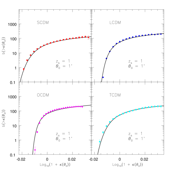
Figure 3: The cumulative bias function $b(>\kappa(\theta_{0}))$ is plotted against the smoothed convergence field $\kappa(\theta_{0})=\kappa_{s}$. The different panels correspond to the different cosmological models and the smoothing angle $\theta_{0}$ is fixed at $1^{\prime}$. The solid line at each panel correspond to analytical predictions from the hierarchical ansatz. The source redshift $z_{s}$ is fixed at unity.

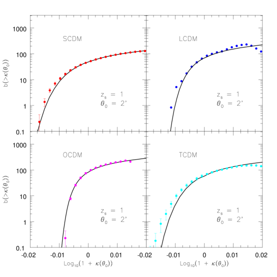
Figure 4: Same as Figure - 3 but for smoothing angle $\theta=2^{\prime}$.

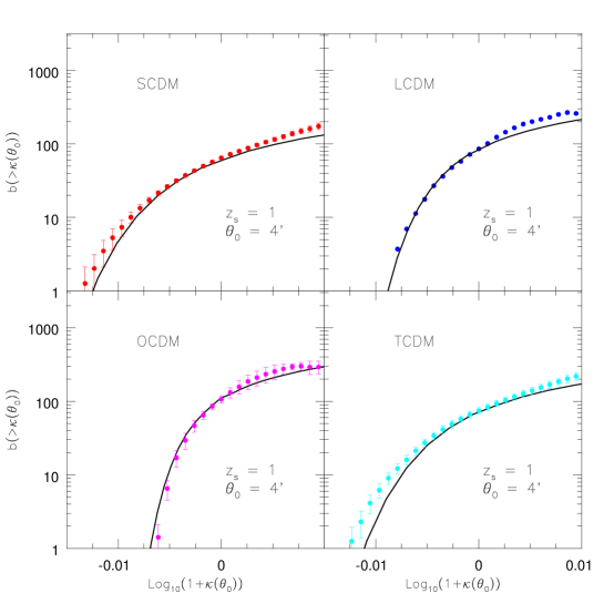
Figure 5: Same as Figure - 3 but for smoothing angle $\theta=4^{\prime}$.

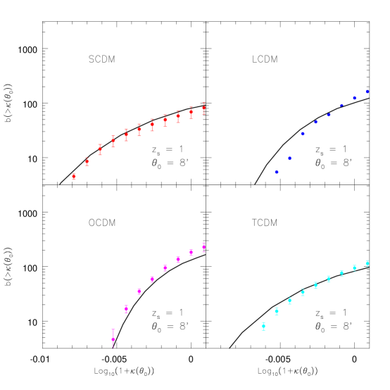
Figure 6: Same as Figure - 3 but for smoothing angle $\theta=8^{\prime}$.

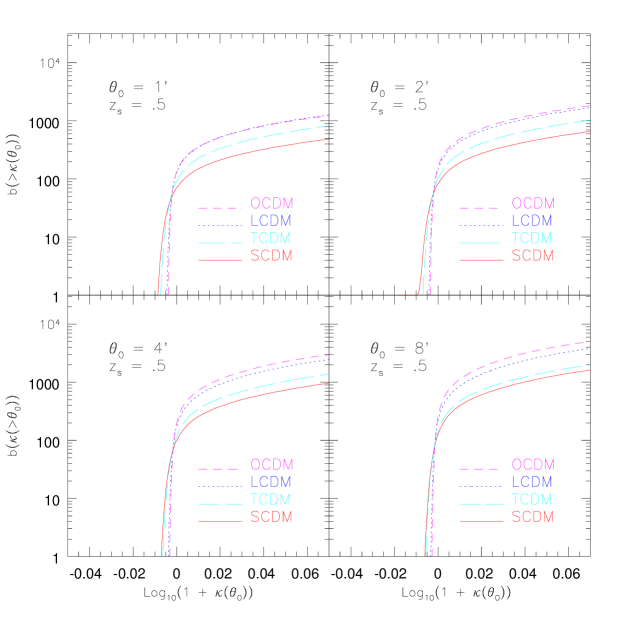
Figure 7: The analytical predictions for the bias associate with the convergence field $\kappa(\theta_{0})$ is plotted as a function of $\kappa(\theta_{0})$. The smoothing angle varies from 1’ to 8’ as indicated. The source redshift is fixed at $z_{s}=.5$. Different curves correspond to SCDM, LCDM, OCDM and TCDM models.

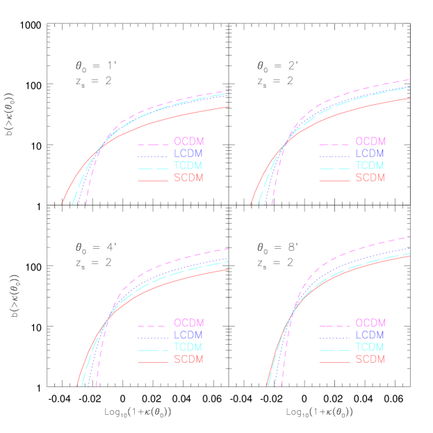
Figure 8: Same as Figure - 7 but for the redshift $z_{s}=2$. Note that the bias associated with high $\kappa(\theta_{0})$ spots in the convergence field decreases as we increase the source redshift $z_{s}$.

4 Comparison against Numerical Ray Tracing Simulations

To compare the analytical results with numerical simulations we have smoothed the convergence field or $\kappa$- map generated from numerical simulations using a top-hat filter of suitable smoothing angle $\theta_{0}$. The minimum smoothing radius we have used is $1^{\prime}$ which is much larger compared to the numerical resolution length scale. In our earlier studies we found that numerical artifacts are negligible even for angles as small as $.25^{\prime}$. The maximum smoothing radius we have studied is $8^{\prime}$, which is much smaller compared to the box size of all models and we expect that the finite volume corrections are not significant in our studies. The box size is L = 166.28’ for the EDS models, L =235.68’ for $\Omega=0.3$ open model and L = 209.44’ for $\Omega=0.3$ model with cosmological constant $\Lambda=0.7$. The numerical outputs from more than ten realizations of these cosmological models were used to find the average and the scatter and were tested against the analytical predictions. For LCDM models we have used only one particular relaisation.

For the determination of the bias from the convergence maps we found that the computation of cumulative bias $b(>\kappa_{s})$ is much more stable compared to the computation of the differential bias $b(\kappa_{s})$. We have therefore used the analytical predictions for $b(>\kappa_{s})$ to compare against numerical simulations. The bias we have studied will represent the correlation of those spots in the convergence maps which are above certain threshold and is defined as:

$$b_{\kappa}(>\kappa_{s})={1\over\sqrt{\langle\kappa_{s}(\gamma_{1})\kappa_{s}(\gamma_{2})\rangle_{c}}}{\left({\int_{\kappa_{s}}^{\infty}d\kappa_{1}\int_{\kappa_{s}}^{\infty}d\kappa_{2}{p_{\kappa}(\kappa_{1},\kappa_{2})}\over\left[\int_{\kappa_{s}}^{\infty}p_{\kappa}(\kappa_{1})d\kappa_{1}\right]^{2}}-1\right)}^{1/2}.$$ (66)

The above expression relies on evaluating bias by finding out directly correlation of points in the convergence map which are above certain threshold and does not depend on any factorization property of bias. We have tested the functional form for the bias as predicted from the analytical model against numerical simulations. The analytical prediction tells us that the bias associated with spots where the smoothed convergence field is negative is very small and is almost zero. On the other hand the negative convergence spots are not biased at all, this property also holds for the bias associated with under-dense regions in the density field which are responsible for producing the negative spots in the convergence field. For positive peaks in the convergence map the bias is positive and it increases sharply as we move towards higher thresholds for $\kappa_{s}$. Contributions to positive spots in the convergence maps comes from density peaks in underlying 3D mass distributions and again its remarkable that the bias associated with both of them are actually described by the same functional form. While we change variables from the reduced convergence $\eta_{s}$ to the actual convergence field $\kappa_{s}$ we introduce a multiplicative factor of $1/k_{min}$. As we explained before that this term introduces the cosmological dependence for the bias in the convergence field. This multiplicative factor is largest for the OCDM model and is smallest for the SCDM model and hence the bias associated with peaks in the convergence maps also follow the same pattern.

The analytical results and results of numerical simulations are plotted in figures - 3-6. Comparing the analytical results with the results obtained from the numerical simulations we find that these predictions match very accurately. The general trend of increase of bias with $\kappa_{s}$ is well reproduced by the analytical models. Also we find that the analytical model is able to describe the relative ordering of the bias function for different cosmological models quite accurately. We have also computed the scatter in numerical results and found them to increase with $\kappa_{s}$. With increasing the threshold we decrease the number of spots which cross that threshold thereby increasing the sample variance. The sample variance also increases with the smoothing length scale $\theta_{0}$ due to decrease in the number of smoothed patches which carry completely independent information. To improve upon the situation we have increased the sampling by shifting the grid used to bin the convergence map in two perpendicular direction. Although there has been several detailed studies to quantify the effect of finite volume correction on the statistics of galaxy clustering, similar studies are still lacking for weak lensing statistics. However it was found in numerical studies clustering that the computed PDF shows a sharp cutoff at some maximum value of cell count $n_{max}$ which is the densest cell in the catalog. Increasing the size of the catalog will increase $n_{max}$ up to which one can reliably compute the PDF. The long exponential tail of PDF also shows large fluctuations due to the presence or absence of any rare dense objects in the N-body catalog. In this paper we have shown how intimately statistics of the weak lensing convergence field $\kappa_{s}$ and its density field counterpart are related. This will indicate that the numerical computations of the one-point PDF and the bias of $\kappa_{s}$ and $\delta$ are both affected in a very similar manner due to the finite size of the catalog. It is therefore quite remarkable that despite the fact that we have not introduced any involved correction procedure in our measurement of bias or PDF the numerical results match the analytical predictions so accurately. We have not studied the factorization property of the bias as predicted by hierarchical ansatz, as there has not been any parallel study in this direction so far dark matter clustering in 3D. However we plan to extend our results to such analysis elsewhere.

We have studied both analytically and numerically how the bias changes if we change the source redshift $z_{s}$. In our earlier studies of PDF we have shown that for low source redshift when one probes the highly non-linear regime directly, the PDF is charecterised by a long exponential tail originating from collapsed objects. Where as if we increase the source redshift we are adding more slabs of matter in the intervening path which are virtually uncorrelated and hence it makes the distribution more Gaussian. However it also increases the variance of the convergence field. We find a similar result for the bias in $\kappa_{s}$ field too, for low source redshift the highly dense spots which are contributing towards the nearby high $\kappa_{s}$spots may also be physically be very near by and hence they themselves may be correlated more strongly than the underlying mass distribution. On the other hand when we increase the source redshift we increase the number of hight density spots which will produce the high convergence $\kappa_{s}$ spots in the map, however it is to be kept in mind that clearly not all these high density spots are in physical proximity in 3D space and might exist in different slabs of the underlying mass distribution. This explains why although the variance of $\kappa_{s}$ and correlation in $\kappa_{s}$ do increase with the source redshift but the bias associated with high $\kappa_{s}$ spots actually decrease with the source redshift.

In our analytical studies we have assumed that the small angle approximation is valid and we also assumed that the separation angle $\theta_{12}$ is much larger than the smoothing angle $\theta_{0}$. This will imply that variance within the smoothed patch is much larger compared to the correlation between the two smoothed patches. However the separation angle should again be small so that we can still replace all spherical harmonics by Fourier modes. In numerical simulations we have placed the smoothed patches separated by an angle at least by thrice the smoothing angle. In almost all cases the separation angle is 3.5 times larger than the smoothing angle. We have also found (as predicted by analytical results) that once the large separation limit is reached the bias function no-longer depends on the separation angle $\theta_{12}$.

5 Discussion

The hierarchical ansatz provides a framework in which gravitational clustering is generally studied in the highly non-linear regime. However most of such earlier studies are directed towards understanding of galaxy clustering and were tested against numerical N-body simulations. However studies based on clustering properties of galaxies are more difficult to interpret as they always depend on a particular biasing scheme employed to relate galaxy population to the underlying mass fluctuation. Forthcoming weak lensing surveys will provide an unique opportunity to directly study matter distribution in the universe and will help us in understanding their clustering properties. The main motivation of this paper is to extend use of hierarchical ansatz to the study of bias as measured from weak lensing surveys.

There have been several studies in which perturbative techniques were used to relate the convergence statistics measured from weak lensing surveys to the clustering statistics of the underlying mass distribution. However analytical predictions based on perturbative techniques normally requires a large smoothing angle. Most of early observational studies of weak lensing surveys will focus on smaller angular scales and hence will require a completely non-linear treatment. In this paper we have shown that our current level of understanding of gravitationally clustering is enough to make concrete predictions for two-point statistics of the convergence field.

We have used the non-local scaling relations to evolve the matter two-point correlation function and used the hierarchical ansatz to relate the higher order correlation function with two-point correlation function. Combined with the generating function approach these two ansatze provide a powerful tool for the analysis of the weak lensing maps and its multi-point statistics. In accompanying papers we have computed the lower order cumulants and the cumulant correlators for various smoothing angle and for different source redshifts (Munshi & Jain 1999a). We have also studied the complete PDF for the smoothed convergence field (Munshi & Jain 1999b). In this paper we have extended these studies by testing analytical predictions for the bias against numerical simulations. The cumulant correlators are nothing but lower order moments of the bias function which we have studied in this paper. We found a very good agreement between analytical results and ray tracing simulations.

The bias which we have studied here is induced by gravitational clustering. It is known from earlier studies that such a bias occurs naturally both in the quasi-linear (Bernardeau 1994) and the highly non-linear regime for over-dense objects (Bernardeau & Schaeffer 1992, 1999, Munshi et al. 1999a,b). It is factorizable and will only depend on the scaling parameters $x$ associated with collapsed objects. We have extended such analytical studies for the weak-lensing convergence field and have shown that similar results do indeed hold even for such cases. Our numerical study confirms such analytical claims and also shows that the functional form for the bias associated with the convergence field is exactly same as that for over-dense spots in underlying mass distribution, so measurement of the bias from weak lensing observations will provide a direct probe into the bias associated with over-dense dark objects in the underlying mass distribution as induced by gravitational clustering. This will help us to separate the contribution to the bias due to gravitational clustering from the bias associated with other non-gravitational sources involved in galaxy formation process.

Although our formalism (which is based on formalism developed by Bernardeau & Schaeffer (1992)) relates the bias of overdense cells in density field with “hot-spots” of the convergence map. Similar results can be obtained by using the extended Press-Schechter formalism to relate the peaks in the convergence field directly with the bias associated with collapsed halos. A detailed analysis will be presented elsewhere.

The hierarchical ansatz not only provides the two-point correlation function (i.e. the bias which we have studied here) for the over-dense objects but it also provides a recipe for computing the higher order correlation functions and the associated cumulants and cumulant correlators. Our formalism which we have developed here can directly be extended to compute such quantities in the highly non-linear regime i.e. at small smoothing angle. However a detailed error analysis is necessary to study the possibility of estimating such quantities from weak lensing observations.

Our analytical results use the top-hat filter, however it was pointed out before that the compensated filter is more suitable for observational studies. We plan to extend our analytical and numerical studies for other filters and results will be presented elsewhere. However it should be kept in mind that although nearby cells do have correlated convergence fields after smoothing with the top-hat window, such correlations are much less significant for the compensated filter (a property which makes it more suitable for the observational purposes for PDF studies).

It is clear that the Born approximation is a necessary ingredient in the analytical computation which we have undertaken in this paper. The Born approximation neglects all the higher order terms in the photon propagation equation. It is then obvious that any statistical quantity such as the higher order cumulants and the cumulant correlators will have correction terms which are neglected in our approach. In the quasi-linear regime i.e. for large smoothing length scales these correction terms can in fact be evaluated using perturbative calculations. However such an approach is not possible to adopt in the highly non-linear regime, because in small angular scales where most contribution comes from length scales with variance well above unity the whole perturbative analysis breaks down and the only way we can check such an approximation is to compare analytical predictions against numerical simulations. Earlier studies of lower order cumulant correlators confirmed that such correction terms are indeed negligible even in small smoothing angle (Munshi & Jain 1999b). A very good match that we have found for the bias function in this study shows that such correction terms are indeed negligible at arbitrary order.

References

- [1] Babul, A., Lee, M.H., 1991, MNRAS, 250, 407
- [2] Balian R., Schaeffer R., 1989, A& A, 220, 1
- [3] Bartelmann M., Huss H., Colberg J.M., Jenkins A.
- [4] Bartelmann, M., Schneider, P., 1991, A& A, 248, 353 Pearce F.R., 1998, A&A, 330, 1
- [5] Bartelmann, M., Schneider, P., 1999, astro-ph/9912508
- [6] Bernardeau F., 1992, ApJ, 392, 1
- [7] Bernardeau F., 1999, astro-ph/9901117
- [8] Bernardeau F., Schaeffer R., 1992, A& A, 255, 1
- [9] Bernardeau F., Schaeffer R., 1999, astro-ph/9903087
- [10] Bernardeau F., van Waerbeke L., Mellier Y., 1997, A& A, 322, 1
- [11] Blandford R.D., Saust A.B., Brainerd T.G., Villumsen J.V., 1991, MNRAS, 251, 600
- [12] Boschan P., Szapudi I., Szalay A.S., 1994, ApJS, 93, 65
- [13] Coles, P., Melott, A., Munshi,D., 1999, ApJL,
- [14] Colombi, S., Bouchet, F.R., & Schaeffer, R., 1992 A&A, 263, 1
- [15] Colombi, S., Bouchet, F.R., & Schaeffer, R., 1994 A&A, 283,301
- [16] Colombi, S., Bouchet, F.R., & Schaeffer, R., 1995 ApJS, 96,401
- [17] Couchman H.M.P., Barber A.J., Thomas P.A., 1998, astro-ph/9810063
- [18] Davis M., Peebles P.J.E., 1977, ApJS, 34, 425
- [19] Diaferio A., Kauffmann G, Colberg J.M., White S.D.M, 1999, MNRAS, 307, 537
- [20] Fry, J.N., 1984, ApJ, 279, 499
- [21] Fry, J.N., Peebles, P.J.E., 1978, ApJ, 221, 19
- [22] Groth, E., Peebles, P.J.E., 1977, ApJ, 217, 385
- [23] Gunn, J.E., 1967, ApJ, 147, 61
- [24] Hamilton A.J.S., Kumar, P., Lu, E. & Matthews, A., 1991, ApJ, 374, L1
- [25] Hui, L., astro-ph/9902275
- [26] Hui, L., Gaztanaga, astro-ph/9810194
- [27] Jain, B., Mo H.J., White S.D.M., 1995, MNRAS, 276, L25
- [28] Jain, B., Seljak, U., 1997, ApJ, 484, 560
- [29] Jain, B., Seljak, U., White, S.D.M., 1998, astro-ph/9804238
- [30] Jain, B., Seljak, U., White, S.D.M., 1999a, astro-ph/9901191
- [31] Jain, B., Seljak, U., White, S.D.M., 1999b, astro-ph/9901287
- [32] Jaroszyn’ski, M., Park, C., Paczynski, B., Gott, J.R., 1990, ApJ, 365, 22
- [33] Jaroszyn’ski, M. 1991, MNRAS, 249, 430
- [34] Kaiser, N., 1992, ApJ, 388, 272
- [35] Kaiser, N., 1998, ApJ, 498, 26
- [36] Kauffmann G, Colberg J.M., Diaferio A., White S.D.M, 1999a, MNRAS, 303, 188
- [37] Kauffmann G, Colberg J.M., Diaferio A., White S.D.M, 1999b, MNRAS, 307, 529
- [38] Limber D.N., 1954, ApJ, 119, 665
- [39] Lee, M.H., Paczyn’ski B., 1990, ApJ, 357, 32
- [40] Miralda-Escudé J., 1991, ApJ, 380, 1
- [41] Munshi D., Bernardeau F., Melott A.L., Schaeffer R., 1999, MNRAS, 303, 433
- [42] Munshi D., Melott A.L, 1998, astro-ph/9801011
- [43] Munshi D., Coles P., Melott A.L., 1999a, MNRAS, 307, 387
- [44] Munshi D., Coles P., Melott A.L., 1999b, MNRAS, 310, 892
- [45] Munshi D., Melott A.L., Coles P., 1999c, MNRAS, 311, 149
- [46] Munshi D., Coles P., 1999a, MNRAS, in press, astro-ph/9911008
- [47] Munshi D., Coles P., 1999b, MNRAS, submitted
- [48] Munshi D., Jain B., 1999a, MNRAS, submitted
- [49] Munshi D., Jain B., 1999b, MNRAS, submitted, astro-ph/9911502
- [50] Mellier Y., 1999, astro-ph/9901116
- [51] Nityananda R., Padamanabhan T., 1994, MNRAS, 271, 976
- [52] Padmanabhan T., Cen R., Ostriker J.P., Summers, F.J., 1996, ApJ, 466, 604
- [53] Premadi P., Martel H., Matzner R., 1998, ApJ, 493, 10
- [54] Press, W.H., Schechter, P. 1974, ApJ, 187, 425
- [55] Peebles P.J.E., 1980, The Large Scale Structure of the Universe. Princeton University Press, Princeton
- [56] Reblinsky, K., Kruse, G., Jain, B., Schneider, P., astro-ph/9907250
- [57] Schneider, P., Weiss, A., 1988, ApJ, 330,1
- [58] Schneider, P., van Waerbeke, L., Jain, B. & Kruse, G. 1998, MNRAS, 296, 873, 873
- [59] Scoccimarro R., Colombi S., Fry J.N., Frieman J.A., Hivon E., Melott A.L., 1998, ApJ, 496, 586 astro-ph/9811184
- [60] Szapudi I., Colombi S., 1996, ApJ, 470, 131
- [61] Szapudi I., Szalay A.S., 1993, ApJ, 408, 43
- [62] Szapudi I., Szalay A.S., 1997, ApJ, 481, L1
- [63] Szapudi I., Szalay A.S., Boschan P., 1992, ApJ, 390, 350
- [64] Valageas, P., Lacey, C., Schaeffer, R., 1999, astro-ph/9902320
- [65] Valageas, P., 1999a, astro-ph/9904300
- [66] Valageas, P., 1999b, astro-ph/9911336
- [67] van Waerbeke, L., Bernardeau, F., Mellier, Y., 1998, astro-ph/9807007
- [68] Wambsganss, J., Cen, R., Ostriker, J.P., 1998, ApJ, 494, 298
- [69] Wambsganss, J., Cen, R., Xu, G. Ostriker, J.P., 1997, ApJ, 494, 29
- [70] Wambsganss, J., Cen, R., Ostriker, J.P., Turner, E.L., 1995, Science, 268, 274
- [71] Wang Y., 1999, ApJ, in press.
- [72] White S.D.M, 1979, MNRAS, 186, 145