The Effect of Resistivity on the Nonlinear Stage of the Magnetorotational Instability in Accretion Disks

Abstract

We present three-dimensional magnetohydrodynamic simulations of the nonlinear evolution of the magnetorotational instability (MRI) with a non-zero Ohmic resistivity. The simulations begin from a homogeneous (unstratified) density distribution, and use the local shearing-box approximation. The evolution of a variety of initial field configurations and strengths is considered, for several values of constant coefficient of resistivity $\eta$. For uniform vertical and toroidal magnetic fields we find unstable growth consistent with the linear analyses; finite resistivity reduces growth rates, and, when large enough, stabilizes the MRI. Even when unstable modes remain, resistivity has significant effects on the nonlinear state. The properties of the saturated state depend on the initial magnetic field configuration. In simulations with an initial uniform vertical field, the MRI is able to support angular momentum transport even for large resistivities through the quasi-periodic generation of axisymmetric radial channel solutions rather than through the maintenance of anisotropic turbulence. Reconnective processes rather than parasitic instabilities mediate the resurgent channel solution in this case. Simulations with zero net flux show that the angular momentum transport and the amplitude of magnetic energy after saturation are significantly reduced by finite resistivity, even at levels where the linear modes are only slightly affected. The MRI is unable to sustain angular momentum transport and turbulent flow against diffusion for $Re_{M}\mathrel{\vbox{\offinterlineskip\hbox{$<$} \kern 1.29167pt\hbox{$\sim$}}}10^{4}$, where the Reynolds number is defined in terms of the disk scale height and sound speed, $Re_{M}=c_{s}H/\eta$. As this is close to the Reynolds numbers expected in low, cool states of dwarf novae, these results suggest that finite resistivity may account for the low and high angular momentum transport rates inferred for these systems.

1 Introduction

In recent years a more complete understanding of the origin of angular momentum transport and turbulence in accretion disks has emerged. The discovery that weak magnetic fields render a differentially rotating plasma unstable (Balbus & Hawley 1991; 1992) has directed the focus of research efforts to magnetohydrodynamic (MHD) processes and the onset and evolution of the magnetorotational instability (MRI). The MRI is a linear, local instability whose existence is independent of both field orientation and strength. The action of the MRI directly produces outward angular momentum transport, as required for accretion disks to accrete.

Studies of the nonlinear evolution and saturation of the MRI are required in any comparison between theory and observation; such studies rely on numerical MHD simulations. Many such numerical investigations have been carried out in recent years. Local three-dimensional MHD simulations have shown that turbulence is initiated and sustained by the MRI (Hawley, Gammie, & Balbus 1995, hereafter HGB; Brandenburg et al. 1995; Stone et al. 1996), and that this turbulence supports a significant outward flux of angular momentum. Both the turbulent energy and angular momentum fluxes are dominated by Maxwell rather than Reynolds stress. Simulations that begin with a vanishing mean flux have been used to examine the implications of the MRI for dynamo action in accretion disks (Brandenburg et al. 1995; Hawley, Gammie, & Balbus 1996, hereafter HGB2) These have demonstrated that the MRI is capable of amplifying and sustaining an initially weak magnetic field for many resistive decay times, thus satisfying the minimum definition of a dynamo. Moreover, these studies show that this process cannot be described by kinematic dynamo theory: the effect of the Lorentz force on the flow can never be ignored, even when the field is weak. A comprehensive review of these and many other results pertaining to the MRI and angular momentum transport in accretion disks is given by Balbus & Hawley (1998, hereafter BH).

Most of the numerical studies of the nonlinear stage of the MRI reported to date have adopted the assumption of ideal MHD, i.e. infinite conductivity, so that the field is perfectly frozen-in to the gas. However, in cold, dense plasmas such as might be expected at the centers of protostellar disks (Stone et al. 1998), or disks in dwarf novae systems (Gammie & Menou 1997), the ionization fraction may become so small that this approximation no longer holds. Obviously, the appropriate representation of some region of interest within a partially ionized plasma depends on the specific densities, temperatures, and ionization fractions therein. Different nonideal MHD effects can be important for different physical conditions (see, e.g., Parker 1979). For example, the ambipolar diffusion regime occurs when the neutral-ion collision time is too long to prevent the gas from drifting across magnetic field lines; generally this corresponds to low densities and ionization fractions (more precisely, when the ratio ${\cal R}$ of the product of the ion and electron gyrofrequencies to the product of the electron-neutral and ion-neutral collision frequencies is ${\cal R}>1$). The linear properties of the MRI in the ambipolar diffusion limit have been studied in detail by Blaes & Balbus (1994). Their primary conclusion is that the MRI will grow provided the neutral-ion collision frequency is greater than the orbital frequency. The resistive regime occurs when collisions between the charge carrying species and neutrals damp electric currents (and therefore magnetic fields) in the plasma, a process equivalent to Ohmic resistivity. Resistive effects generally dominate in high density but weakly ionized plasmas (more precisely, when ${\cal R}<1$). The local linear stability properties of the MRI with simple resistivity have been examined for both vertical fields (Jin 1996; BH) and toroidal fields (Papaloizou & Terquem 1997). The global stability of resistive disks has been examined by Sano & Miyama (1999). The effect of resistivity on the linear instability is straightforward: if Ohmic diffusion is sufficiently rapid, it can stabilize the MRI. Recently Wardle (1999) has explored the linear properties of the MRI in the a third regime where the conductivity tensor is dominated by the Hall effect. In this limit the MRI exhibits interesting new behavior, including a loss of symmetry with respect to the sign of the background magnetic field.

Just as the linear properties of the MRI in these regimes have been investigated, the nonlinear evolution has also been simulated for a variety of limits. In the so called “strong-coupling limit” (in which the ion inertia is ignored, and the ion density is assumed to be a simple power law of the neutral density), the effect of ambipolar diffusion is to add a nonlinear diffusion term to the induction equation. As a test of a numerical algorithm to solve this term, MacLow et al (1995) reported two-dimensional simulations of the initial growth of the MRI; their results were in agreement with the stability criterion derived by Blaes & Balbus (1994). Brandenburg et al. (1995) performed three-dimensional simulations of the MRI in stratified disks; some of their models included the effects of ambipolar diffusion. They found that sufficiently large diffusivity could damp the MHD turbulence, consistent with the conclusions of Blaes & Balbus (1994).

Hawley & Stone (1998) carried out a full ion-neutral simulation of the MRI in weakly ionized plasmas, where the ions and neutrals are treated as separate fluids coupled only through a collisional drag term. Although they found close agreement with the Blaes and Balbus linear results, the structure and evolution of the saturated state of the MRI in weakly coupled fluids is more complex. Full turbulence is produced only when the collision frequency is $\mathrel{\vbox{\offinterlineskip\hbox{$>$} \kern 1.29167pt\hbox{$\sim$}}}100$ times the orbital frequency. At lower collision frequencies, the nonlinear turbulence is increasingly inhibited by the neutrals, resulting in significantly lowered angular momentum transport rates. These results illustrate that it is possible for nonideal effects to have significant consequences for the nonlinear evolution even when their impact on the linear instability is slight.

The nonlinear evolution of a differentially rotating flow with a nonzero resistivity represents a more straightforward simulation regime. In their study of dynamo action associated with the MRI, HGB2 presented two simulations in which explicit resistive effects were included. These indicated that saturation amplitude and angular momentum transport rates could be significantly decreased by a large resistivity. More recently, Sano, Inutsuka, & Miyama (1998; hereafter SIM) explored saturation of the 2D channel solution in the presence of strong resistivity. They found reconnection of magnetic field lines across the channels could act as a saturation mechanism.

In this paper we will explore in greater depth the nonlinear behavior of the MRI in a single fluid with a finite resistivity. We present an extensive series of resistive MHD simulations in three-dimensions. We study a variety of initial field configurations and strengths over a wide range of resistivities. We find that there are substantial differences between the nonlinear evolution of the MRI in the presence of a net flux compared to the evolution at the resistivity with zero volume-averaged flux. This behavior arises because Ohmic dissipation can never destroy a net field, i.e., one which is supported by currents outside the simulation domain.

As has already been pointed out (BH), a critical dimensionless parameter which may control the behavior of the MRI in dissipative disks is the magnetic Prandtl number, i.e., the ratio of the coefficients of viscosity and resistivity. The present study does not include a physical viscous dissipation; some effective viscous dissipation is, of course, already present due to numerical effects. Thus, the exploration of the role of magnetic Prandtl number in determining the nonlinear outcome of the MRI must await future studies.

This paper is organized as follows. In §2, we discuss our numerical method (including the extension of the ZEUS algorithm to model highly resistive plasmas), and initial and boundary conditions that characterize the simulations. In §3, we discuss the results of simulations with uniform vertical fields, vertical fields with zero net flux, and uniform azimuthal fields. Our conclusions are presented in §4.

2 Method

2.1 Equations and Algorithms

Our computational model is based on the shearing box approximation developed by HGB. This approximation uses a local expansion of the equations of motion about a fiducial point of radius $R_{\circ}$ in cylindrical coordinates $(R,\phi,z)$. By considering a region whose extent is much less than $R_{\circ}$, one can define a local set of Cartesian coordinates $x=R-R_{\circ},y=R_{\circ}(\phi-\Omega t),z=z$ that corotate with the disk. Using $|x|/R_{\circ}\ll 1$, we expand the equations of motion to first order in $|x|/R_{\circ}$ to obtain the local equations of compressible MHD (HGB):

$${{\partial\rho}\over{\partial t}}+{\bf\nabla}\cdot(\rho{\bf v})=0$$ (1)

$${{\partial{\bf v}}\over{\partial t}}+{\bf v}\cdot\nabla{\bf v}=-{1\over\rho}\nabla\left(P+{B^{2}\over 8\pi}\right)+{{{\bf B}\cdot\nabla{\bf B}}\over 4\pi\rho}-2{\bf\Omega}\times{\bf v}+3\Omega^{2}x{\bf{\hat{x}}}$$ (2)

$${\partial{\bf B}\over{\partial t}}={\bf\nabla}\times[({\bf v}\times{\bf B})-\eta{\bf J}],$$ (3)

$${\partial{\rho\epsilon}\over{\partial t}}+{\bf\nabla}\cdot(\rho\epsilon{\bf v})+P({\bf\nabla}\cdot{\bf v})-\eta\bf J^{2}=0$$ (4)

where $\epsilon$ is the specific internal energy, ${\bf J}={\bf\nabla}\times{\bf B}$ is the current density, and the other symbols have their usual meaning. For our study, the magnetic diffusivity $\eta$ is spatially uniform and time independent. The $z$ component of gravity is ignored; consequently, there are no vertical buoyancy effects. We adopt an adiabatic equation of state

$$P=\rho\epsilon(\gamma-1)$$ (5)

with $\gamma=5/3$. A hydrodynamic equilibrium solution to equations (1)–(4) is constant density and pressure and a uniform shear flow, ${\bf v}=-(3/2)\Omega x{\bf{\hat{y}}}$.

The shearing box approximation employs strictly periodic boundary conditions in the angular ($y$) and vertical ($z$) directions, and shearing-periodic boundary conditions in the radial ($x$) direction. These boundary conditions and their implementation are described in more detail in HGB. Briefly, faces along the $x$ directions are periodic initially but subsequently shear with respect to each other. Any fluid element that travels off the outer radial boundary reappears at the lower radial boundary at the corresponding sheared position.

The above equations of MHD are solved using the ZEUS code (Stone and Norman 1992a; 1992b). ZEUS is a time explicit MHD code based on finite differences that uses the Method of Characteristics – Constrained Transport (MOCCT) algorithm (Hawley & Stone 1995) to evolve both the induction equation and the Lorentz force. The advantage of MOCCT is that it evolves the magnetic field in such a way as to maintain the constraint $\nabla\cdot\bf{B}=0$. Key to this property is the use of Stoke’s Law to write the induction equation in integral form: the rate of change of the magnetic flux through any face of a computational zone is then simply the line integral of the electromotive force (emf) around the edges of the face (Evans & Hawley 1988). To extend the method to include resistivity, we use an operator split solution procedure in which the MOCCT technique is used to update the first term on the RHS of (3) and then the constrained transport formalism is again used to update the magnetic flux using an effective emf defined by the resistive term (i.e. $-\eta\bf{J}$). The current ${\bf J}$ used in this step is computed from the partially updated field resulting from the MOCCT step. Resistive heating [i.e. the last term on the LHS of eq. (4)] is computed with this same current, appropriately averaged to the grid center. Since our update of the resistive term is time explicit, we also add a new timestep constraint so that $\bigtriangleup t\leq[\min(\bigtriangleup x,\bigtriangleup y,\bigtriangleup z)]^{2}/\eta$.

We tested our implementation of the resistivity algorithm by following the diffusion of a magnetic field with an initially gaussian profile in a non-rotating box, a problem whose solution is known analytically. As described in §3, we also have reproduced the linear stability criterion for the MRI in resistive differentially rotating flows.

2.2 Initial Conditions

For these simulations we use a computational volume with radial dimension $L_{x}$ = 1, azimuthal dimension $L_{y}=2\pi$, and vertical dimension $L_{z}$ = 1. Most of the runs use a standard grid resolution of $59\times 123\times 59$. (Note that this resolution is comparable to the high-resolution runs of HGB and HGB2. The increase in what constitutes a standard grid resolution simply reflects the increase in computational power over the last few years.) Initially the computational domain is filled with a uniform plasma of density $\rho_{0}=1$ and pressure $P_{0}=10^{-6}$. We set $\Omega=10^{-3}$, sound speed $c_{s}=(\gamma P/\rho)^{1/2}$ and vertical scale height $H=c_{s}/\Omega\approx 1.3$. We study the evolution of a variety of initial magnetic field configurations including constant vertical fields $B_{z}$, constant toroidal fields $B_{y}$, and spatially varying $B_{z}$ fields whose volume-average sums to zero (“zero-net field”). The initial magnetic field strength $B_{0}$ is specified by $\beta=P_{0}/(B_{0}^{2}/8\pi)$.

Each of these initial field configurations is evolved using a range of resistivities $\eta$. The importance of a specific value of resistivity is characterized by the magnetic Reynolds number $Re_{M}$, defined as a characteristic length times velocity divided by $\eta$. Here we define $Re_{M}$ in terms of important disk length and velocity scales, namely, the disk sound speed and vertical scale height,

$$Re_{M}\equiv\frac{Hc_{s}}{\eta}.$$ (6)

With this definition, the magnetic Reynolds number is independent of the initial magnetic field. An alternative definition uses the wavelength of the fastest growing mode of the MRI ($\sim v_{A}/\Omega$) and $v_{A}$ as the characteristic length and velocity,

$$Re_{M}^{\prime}=\frac{v_{A}^{2}}{\Omega\eta}.$$ (7)

This definition was used by Sano et al. (1998). The two definitions are related by $Re_{M}=Re_{M}^{\prime}\beta/2$ using the parameter $\beta=2c_{s}^{2}/v_{A}^{2}$.

The essential properties of resistive MRI can be understood from simple physical scalings. In the nonresistive limit the MRI’s fastest growing wavenumber has $k\cdot v_{A}\approx\Omega$. For a given resistivity $\eta$ the magnetic field diffusion rate will be of order $k^{2}\eta$. The MRI will be strongly affected at wavenumbers where the resistive damping rate exceeds the MRI linear growth rate. An important demarcation point is established by setting the resistive damping wavenumber $k_{D}$, defined to be that wavenumber where the diffusion rate is equal to $\Omega$, equal to the wavenumber of the fastest growing MRI mode, $k_{MRI}=\Omega/v_{A}$. This occurs when $Re_{M}^{\prime}=1$, or

$$Re_{M}=\beta/2.$$ (8)

In addition to the critical Reynolds number, established by $k_{D}=k_{MRI}$, one can define other important limits. Because the resistive damping rate is proportional to the square of the wavenumber, the largest wavenumbers (shortest wavelengths) of the MRI will be affected first. Small wavenumbers have the potential to remain unstable for larger resistivities. In the small wavenumber (large wavelength) limit, the growth rate of the MRI is proportional to $k\cdot v_{A}$. If we equate this growth rate to the resistive damping rate we obtain the condition $v_{A}/k\eta=1$. Thus, for a given scale $H$, it is possible to damp all modes with $k\geq 2\pi/H$, and completely suppress the MRI, if

$$Re_{M}=2\pi{c_{s}\over v_{A}}\propto\beta^{1/2}.$$ (9)

In a numerical simulation, the largest available scale is set by the dimensions of the computational domain, $L$, and this stability limit would also be proportional to the ratio $H/L$. In any case, when the diffusion wavenumber is $k_{D}=2\pi/L$ the entire computational box would be dominated by diffusion on a timescale $\Omega$. This Reynolds number is

$$Re_{M}=\left({2\pi\over L}\right)^{2}\left({Hc_{s}\over\Omega}\right)=(2\pi H/L)^{2}\sim 40(H/L)^{2}.$$ (10)

At the other extreme we can also define a Reynolds number for which the diffusion wavenumber is $k_{D}=2\pi/\Delta x$, where $\Delta x$ is the size of a grid zone. For a computational grid size $L$ divided into $N$ grid zones the gridscale Reynolds number is

$$Re_{M}=(2\pi)^{2}(HN/L)^{2}.$$ (11)

For Reynolds numbers larger than this, diffusion will not be the dominant effect on dynamical timescales for all computationally resolved lengthscales. The magnetic Reynolds numbers used for our investigations below are all smaller than this limit.

Our numerical simulations also possess an intrinsic numerical resistivity due to truncation error. Because the numerical resistiviy is a nonlinear function of the grid spacing, it must be measured for each individual application by increasing the magnitude of the physical resistivity from zero and noting at what point the solution diverges from the ideal case. As described in section 3.2, we find for our standard resolution our numerical Reynolds number is about 50,000 for vertical fields with zero net flux.

3 Results

3.1 Uniform Vertical Fields

We begin with simulations of an initial weak uniform poloidal magnetic field in the shearing box. Due to periodic boundary conditions, the net flux associated with this initial mean field remains unchanged for all times. Hawley & Balbus (1992) simulated this problem in 2D in the ideal MHD limit and found that the instability produced an exponentially growing “channel solution” consisting of two oppositely directed radial streams surrounded by radial magnetic field. In 2D, saturation of the instability does not occur; instead, simulations terminate when the plasma channel is squeezed into a thin sheet too small to resolve. In 3D, however, the channels break down into MHD turbulence due to nonaxisymmetric “parasitic” instabilities (Goodman & Xu 1994; HGB; HGB2) so long as the vertical wavelength of the channel mode is less than the radial size of the computational domain.

Even in 2D, however, additional possibilities are created by the addition of a finite resistivity. SIM carried out 2D simulations of the vertical field problem with a resistive plasma for a variety of field strengths, and for resistivities $0.3\leq Re_{M}^{\prime}\leq 3$ [using the definition of Reynolds number given by eq. (7)]. They found an interesting dichotomy of behavior depending on whether or not $Re_{M}^{\prime}$ was greater or less than one (the critical value). When $Re_{M}^{\prime}<1$, the channel solution saturates via magnetic diffusion and reconnection across the radial streams. Assuming that the resistivity was not so large as to stabilize all possible wavelengths within the computational domain, simulations with $Re_{M}^{\prime}<1$ amplified the magnetic field until $Re_{M}^{\prime}\sim 1$ at which point saturation occurred. For stronger initial fields, however, or with weak resistivity such that $Re_{M}^{\prime}>1$ SIM found that the 2D channel solution remained as before, growing without apparent limit. Since saturation by parasitic modes is inherently a nonaxisymmetric process, 3D resistive simulations are required to explore this regime.

In this section we consider a constant vertical magnetic field in an initially uniform 3D shearing box. The linear dispersion relation for a vertical field with resistivity is given by Jin (1996). Ignoring buoyancy terms and assuming a Keplerian background and a displacement ${\bf k}=k\hat{z}$, a simplified linear dispersion relation can be written

$$\sigma^{4}+2\xi\sigma^{3}+(2q^{2}+\xi^{2}+1)\sigma^{2}+2\xi(q^{2}+1)\sigma-3q^{2}+q^{4}+\xi^{2}=0$$ (12)

where $\sigma$ is a growth rate in units of orbital frequency, $q=k_{z}v_{A}/\Omega$, and $\xi=k_{z}^{2}\eta/\Omega$. Growth rates as a function of $q$ and $\xi$ are plotted in Figure 1.

In a fully conducting plasma, the fastest growing mode of the MRI has $q=\sqrt{15}/4$; the corresponding wavelength $\lambda_{c}$ is given by

$$\lambda_{c}=2\pi\sqrt{16/15}|{\bf v_{A}}|/\Omega.$$ (13)

For these uniform vertical field simulations we select $\beta=400$, $\lambda_{c}$ = 0.459. This wavelength extends over 27 grid cells so fast-growing modes are well resolved. The largest vertical wavelength allowed in the box is $\lambda=L$ which corresponds to $q=0.444$ and has a growth rate of $\sigma=0.57$. Wavelengths $L/2$ ($q=0.888$) and $L/3$ ($q=1.332$) are also unstable with growth rates $\sigma=0.75$ and 0.66 respectively. The zero resistivity run serves as a control model; it uses the same parameters (although a slightly different numerical resolution) as the run labeled Z4 in HGB. We have run four resistive simulations with this initial magnetic field using $Re_{M}=1300$, 520, 260, and 130. For increasing values of magnetic resistivity the most unstable wavelength shifts to larger scales and the growth rate is substantially lower than the ideal MHD rate. The linear growth rates for the three largest wavelengths with $Re_{M}=1300$ are $\sigma=0.53$, 0.62, and 0.41. From the dimensional analysis of the critical magnetic Reynolds number, for our given field strength and box size, we expect that the growth rate of the MRI should be significantly affected for $Re_{M}\sim\beta=400$. Indeed, at that level $\lambda=L/3$ is no longer unstable, and the growth rates for $\lambda=L$ and $L/2$ are reduced to 0.45 and 0.36. At $Re_{M}=260$ only the $\lambda=L$ wavelength remains unstable with a growth rate of 0.37. This wavelength too becomes marginally stable for $Re_{M}=130$.

Figure 2 is a plot of the time evolution of the volume averaged total magnetic energy in each run. In keeping with the linear analysis, we find no growth when $Re_{M}=130$; all modes have been stabilized by resistivity. Unstable modes are present for all other values of $Re_{M}$, with the most rapid growth for the non-resistive ($\eta=0$) model. For each of the models in which unstable modes are present, the evolution of the magnetic energy is similar. An initial phase of exponential growth ends in a sharp peak, after which the magnetic energy declines rapidly before fluctuating about a lower average level. For $\eta=0$, this initial peak occurs at 3.5 orbits. Consistent with the decrease in linear growth rates, the peak occurs at increasingly later times for decreasing $Re_{M}$; for $Re_{M}=260$ the magnetic energy peaks at 8 orbits.

In the absence of resistivity, the initial linear growth is associated with development of the channel solution at the wavelength of the fastest growing mode; for $\eta=0$ this is $L_{z}/2$. This is also the fastest growing wavelength in the $Re_{M}=1300$ model, which behaves similarly. The growth rate for the $Re_{M}=1300$ run is $80\%$ of the maximum growth rate for ideal MHD (0.75$\Omega$), close to what is predicted by the linear analysis. The $\lambda=L/2$ channel solution is well established by orbit 2.2 for $\eta=0$ and 3.2 for $Re_{M}=1300$. A spectral analysis at this stage indicates that the magnetic energy of the fastest growing wavenumber mode is 3 orders of magnitude greater than all other modes combined.

In the runs with $Re_{M}=520$ and 260, the linear growth rates have been reduced by magnetic diffusion enough to change the nature of the observed channel solution. Ohmic dissipation stabilizes small scale perturbations, and we no longer observe the $\lambda=L_{z}/2$ mode; the dominant mode is now $\lambda=L$, i.e., a two stream (one in, one out) mode. With $Re_{M}=260$ the growth rate of this mode has decreased to $48\%$ of the ideal MHD value.

As resistivity is increased, the peak in the magnetic energy at the end of the linear growth phase achieves higher amplitudes. This suggests that the fastest growing modes of the parasitic instabilities (the Kelvin-Helmholtz modes) are also affected by resistivity (Goodman & Xu 1994). One reason for this is that the parasitic modes require vertical wavenumbers that are larger than radial wavenumbers. For $Re_{M}$ less than 260, resistivity restricts growth to the smallest vertical wavenumber, inhibiting the onset of the parasitic instability. This allows the channel solution to persist and to reach higher amplitudes before disruption.

Following the peak and subsequent decline, the magnetic energy in all models fluctuates around a mean value. Increasing the resistivity (1) reduces this mean saturated field energy, (2) increases the magnitude of the fluctuations relative to the saturation amplitude, and (3) increases the timescale of the fluctuations. Table 1 lists volume-averaged values for a variety of quantities in the saturated state, time-averaged over the last twenty orbits of each run. There is a systematic decline in both kinetic and magnetic energies with increasing resistivity. For the $Re_{M}=260$ model the mean kinetic energy in the turbulent fluctuations is $26\%$ of the mean value in the ideal MHD simulation. In the turbulent flow the magnetic energy resides primarily in the azimuthal component of the field. The background shear flow always favors the growth of the azimuthal field component. The ratio of $B_{y}^{2}$ to $B_{x}^{2}+B_{z}^{2}$ is 2.6 in the zero resistivity run, increases to 3.1 for the $Re_{M}=520$ run before dropping back to 2.6 with $Re_{M}=260$. The magnetic field energy is greater than the perturbed kinetic energy by a factor of 2.4 with no resistivity; this ratio decreases with increasing resistivity, down to 1.24 in the $Re_{M}=260$ run.

Turbulent shear stress $W_{xy}={\rho v_{x}\delta v_{y}-B_{x}B_{y}/4\pi}$ transports angular momentum outward, but the total stress decreases with Reynolds number. Using Shakura-Sunyaev scaling, $W_{xy}=\alpha P_{o}$, $\alpha$ decreases from 0.307 at $\eta=0$ to 0.053 at $Re_{M}=260$. Angular momentum transport is correspondingly reduced. In all cases the Maxwell stress dominates over the Reynolds stress, although the ratio of Maxwell to Reynolds stress decreases from 4.8 for $\eta=0$ to 3.38 for $Re_{M}=260$.

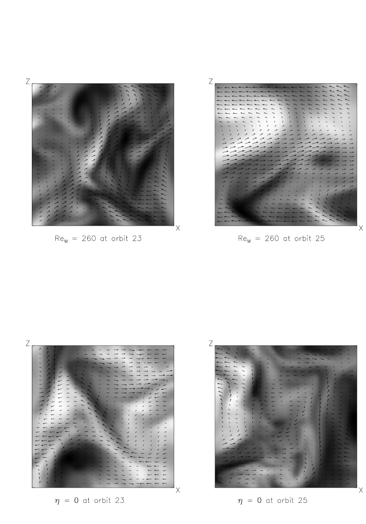
Figure 3: Slices in the $x-z$ plane at $y=0$ of the angular momentum excess (colors) and poloidal magnetic field (arrows) at orbits 24 and 26 in the $Re_{M}=260$ and $\eta=0$ runs. Note the re-emergence of the channel solution in the resistive case.

Although the time histories of these runs (Figure 2) are superficially similar, the late-time state of the $Re_{M}=520$ and 260 simulations is strikingly different than that of the higher $Re_{M}$ runs. In the ideal MHD case, and in the $Re_{M}=1300$ run, the flows are turbulent. At lower $Re_{M}$ values, however, the fluctuations seen in the saturated state are associated with the periodic re-emergence of the channel solution. Figure 3 shows images of the angular momentum excess $\delta L\equiv\rho(v_{y}+1.5\Omega x)$ overlaid by magnetic field lines in the $x-z$ plane at $y=0$ at orbits 23 and 25 in the ideal ($\eta=0$) and $Re_{M}=260$ models. Note from Figure 2 that a strong peak in the magnetic energy begins to develop in the $Re_{M}=260$ model at these times. In the ideal model, the angular momentum excess shows large amplitude, disordered fluctuations; the magnetic field is highly tangled and time-variable, characteristic of MHD turbulence. In contrast, the $Re_{M}=260$ model shows a disordered field and pattern of angular momentum excess at orbit 23, but by orbit 25 (during the growth of the next peak in the magnetic energy) this has changed to a layered profile, combined with a large amplitude sinusoidal variation in the field, both characteristic of the channel solution. A spectral analysis of the magnetic field in the $Re_{M}=260$ model at orbit 25 shows not the power law usually associated with turbulence, but rather the domination of the $\lambda=L_{z}$ mode by two orders of magnitude.

The decrease in turbulent flow and the strength of the resurgent channel solution may be examined by observing the increase in the kinetic energy associated with radial motions. In the $Re_{M}=260$ run, we find that a large increase in the radial kinetic energy accompanies every significant increase in magnetic field energy. For example, at orbit 23 $<\rho v^{2}_{x}>\sim 0.01P_{o}$ however, by orbit 25 the radial kinetic energy has increased to $0.1P_{o}$. The radial kinetic energy rises by at least one order of magnitude every time magnetic field energy peaks.

For $Re_{M}=260$, the channel solution first re-emerges (after the initial peak) at orbit 17, and thereafter occurs roughly every 4 orbits. These recurrent channels saturate not through parasitic instabilities, but by reconnection across the channels. In their 2D simulations, SIM found that reconnection could be an alternative saturation mechanism for the channel solution; we find that this behavior in 3D as well. The resistive diffusion time for variations of lengthscale $L_{z}/2$ (the vertical extent of one channel) is $L_{z}^{2}/4\eta$, or about 6 orbits. The frequency of variability is comparable to this resistive diffusion time.

The quasi-periodic emergence of the channel solution could have important consequences for time variability of the accretion rate in disks. Figure 4 plots the shear stress normalized by the initial pressure ($W_{xy}/P_{0}=\alpha$) for the ideal and $Re_{M}$=260 case. Fluctuations in the stress exceed an order of magnitude, although the mean is less than the ideal MHD case. Note that the stress associated with the initial peak results in $\alpha>1$. We may conclude that for high values of magnetic diffusion in a mean field, the rate of transport is cyclic and highly variable.

Considerable heating due to Ohmic dissipation occurs, particularly in the high resistivity runs. For example, at $Re_{M}=260$ the internal energy rises by a factor of $\sim 100$ during the initial decline from the magnetic energy peak at orbit 8. This is a much greater amount of heating than that seen in the other runs. It would appear that most of the magnetic energy extracted from the differential rotation by the growth of the MRI now heats the disk through Ohmic dissipation. This heating is an indication that resistivity is playing a major role in terminating the channel flow. During the later phase of evolution, the internal energy rises in a somewhat stair-step fashion during each re-emergence of the channel solution, although never again at so large a rate. For example, after saturation the internal energy in the $Re_{M}=260$ simulation rises only another 5% by orbit 40. Again this indicates saturation through resistivity. Ohmic heating also drives changes in the plasma $\beta$ parameter. Since we have a simple adiabatic equation of state, with no radiative losses, heat simply accumulates. Initially the MRI drives $\beta$ toward unity. However, after saturation $\beta$ differs considerably for runs with different resistivity, for example $\eta=0$ $\beta\approx 17$ while for $Re_{m}=260$ $\beta\approx 3000$. In these simulations this heating keeps the magnetic pressure from becoming dynamically important, but has limited importance since there is no vertical gravity. In a disk, radiative cooling would limit the growth of $\beta$.

3.2 Vertical Fields with Zero Net Flux

In the previous section we considered a domain filled with a uniform vertical field. Since the currents generating such a field are outside the computational domain, the background flux cannot change, regardless of the strength of the resistivity. The next set of simulations begins with an initial magnetic field configuration $B_{z}=B_{o}\sin 2{\pi}x$. With periodic (and shearing-periodic) boundary conditions, the mean field $\langle B\rangle$ remains zero for all time. Therefore, unlike the uniform vertical field simulations above, physical resistivity can now completely dissipate the field. This particular initial zero-net field configuration was previously studied in the ideal MHD limit by HGB2.

We describe the results of six runs corresponding to six values of magnetic Reynolds number: $Re_{M}=\infty(\eta=0)$, 65K, 26K, 19.5K, 13K, and 1.3K. These simulations are all performed with a maximum field strength of $\beta=400$ and at our standard resolution. Figure 5 is a plot of the time-evolution of the total magnetic energy for these values of the magnetic Reynolds number. Except for the case of $Re_{M}=1.3$K, an initial period of exponential growth is observed, followed by saturation in a sharp peak near 3.2 orbits. As in the uniform vertical field runs, this rise to a strong peak is associated with the $k_{x}=k_{y}=0$ and $k_{z}=4\pi$ mode, the fastest growing mode from the linear analysis. Note that in all except the ideal MHD case, some diffusion of the initial field can be observed during the first two orbits; for $Re_{M}$=13K and $Re_{M}$=1.3K the field energy is $89\%$ and $24\%$ of its initial value by orbit 2.2. The diffusion is so rapid for the $Re_{M}=1.3$K model that significant growth in the field energy is never attained. The azimuthal and radial components of the magnetic energy peak at $\sim 10^{-5}P_{o}$, only $\sim$ 4 orders of magnitude greater than their values at orbit 0.5. After orbit 4 the energy in both of these components starts to decline. The vertical component does not exhibit any growth at all. Unlike the radial and azimuthal field components any amplification is insignificant compared to the resistive loss. The growth of the linear mode is, in turn, severely restricted when the background field is rapidly diffusing.

As $Re_{M}$ is decreased, there is a small decline in the peak values of azimuthal and radial field energy; it is the vertical field energy that is most affected. At $Re_{M}$=13K the peak value of vertical field energy is only 1.24 times greater then its initial value. Resistivity affects the evolution not so much by altering the growth rates of the most unstable modes, but by diffusing away the background field upon which those modes are growing. This was not a factor in the uniform initial field models, and the decline in the amplitude of the nonlinear flow at saturation as a function of $Re_{M}$ is a consequence.

After the initial peak, the magnetic energies decline to an approximate mean value about which there are large amplitude, short-timescale fluctuations. Because the spatial variation of the field in the initial state causes the wavelength of the fastest growing mode to vary, parasitic instabilities are not required to cause the channel solution to transition to turbulence. Instead, the structure which results from the growth of the linear modes is already complex enough that turbulence is the inevitable outcome. After the initial peak, the MRI saturates as MHD turbulence for all values of $Re_{M}$ except $Re_{M}=1300$.

Table 2 lists the average value in the turbulent state of selected quantities for several runs. Each quantity has been averaged over the time period 30 – 50 orbits. For $\eta=0$, significant growth of the MRI occurs after 2 orbits, with the saturated magnetic energy level $\sim 0.01P_{o}$. At 2.2 orbits, $95\%$ of the field energy is located in the toroidal field. The magnetic energy is dominated by the azimuthal field with $85\%$ of this energy in the azimuthal component. The $Re_{M}$=130K and $Re_{M}$=65K simulations show little apparent difference in energy levels. Angular momentum transport was similar in these three simulations as well, with $\alpha\sim 0.008$. Since there is little difference between resistive runs with $Re_{M}\mathrel{\vbox{\offinterlineskip\hbox{$>$} \kern 1.29167pt\hbox{$\sim$}}}65$K and ideal MHD runs, the effective numerical resistivity would appear to be of the same order, $\sim$ $Re_{M}=65K$.

Below $Re_{M}=65$K, there is a systematic decline in the saturation amplitude with decreasing $Re_{M}$. The magnetic energy is $3\times 10^{-4}P_{0}$ for $Re_{M}=13$K, compared with $10^{-2}P_{o}$ for the ideal MHD run. Angular momentum transport also declines with decreasing Reynolds number. In the $Re_{M}=26$K run the field saturates at levels above the initial energy, with a small but non-negligible transport rate of $\alpha\mathrel{\vbox{\offinterlineskip\hbox{$>$} \kern 1.29167pt\hbox{$\sim$}}}2\times 10^{-3}$. The $Re_{M}=13K$ run is strongly affected. At orbit 3 it has $\alpha$=0.007 and a Maxwell to Reynolds stress ratio = 2.4. The poloidal field is preferentially destroyed as time proceeds; at orbit 3 $53\%$ of the field energy is in the $B_{y}$ component but this increases to $92\%$ by orbit 10. At orbit 30, $\alpha$ = 0.0001 and $99\%$ of the remaining energy is in the $B_{y}$ component. Transport has effectively been shut down in the disk, and Ohmic dissipation allows the field energy to continue decreasing. Although the magnetic energy stops declining beyond orbit 30, the mean magnetic energy and effective $\alpha$ are so small as to imply the MRI is effectively quenched. At this point the field has large scale organized structure. It is layered: in the upper half of the box field is directed toward the positive azimuthal direction, and in the lower half the field is directed toward the negative azimuthal direction.

We expect the dissipational lengthscale to grow as $Re_{M}$ is lowered. This expectation can be examined quantitatively. Figure 6 is a comparison of the power spectrum of fluctuations in the magnetic energy as a function of wavenumber in the y-dimension $k_{y}$ in the $Re_{M}=13K$ and the $\eta=0$ runs. The spectra are time averaged over orbits 15 to 23 for $Re_{M}=13K$ and 16 to 27 for $\eta=0$. The $Re_{M}=13K$ spectrum has been normalized to give it the same amplitude as the $\eta=0$ case. Both spectra are fit by decreasing power laws, with fluctuations on large scales (small k) fit by a Kolmogorov-like slope (-11/3). On small scales (large k), where dissipation becomes important, the slope of the spectra becomes much steeper. For the $Re_{M}=13K$ run, this change in slope occurs at about $k_{y}\sim 8(2\pi)/L_{y}$, while for the ideal run the change does not occur until $k_{y}\sim 11(2\pi)/L_{y}$. Thus, the large explicit resistivity clearly smooths the turbulence on small scales as expected.

In the ideal MHD simulations of HGB2 using an initial vertical field that varies as $\sin(x)$, the energies in the late-time turbulent state were more or less independent of the initial field strength. Here we consider a zero net vertical flux model with $\beta=1600$ initially and $Re_{M}=19.5K$, computed at the standard resolution. The evolution of the magnetic energy is qualitatively similar to the $\beta=400$ model except that the energy levels of the weaker field simulation always remain a factor four times lower throughout the evolution. The field energy is concentrated in the azimuthal component for both runs. Both runs show similar time behavior with respect to angular momentum transport. An average from orbit 4 through orbit 10 yields $\alpha=0.012$ for the $\beta=400$ model; this is five times greater then average transport for the $\beta=1600$ run. The power spectra for these runs are also similar.

One difference between the $\beta=400$ and the weak field $\beta=1600$ simulation shows up clearly in the linear stage. The weak field run has a critical wavelength $\lambda_{c}=L_{z}/4$. This is consistent with linear analysis, which, for $\beta$=1600 predicts a critical wavelength $\lambda_{c}=0.23$. Decreasing the field strength while keeping $Re_{M}$ and the box size fixed simply shifts the wavelength of the most unstable mode down closer to the resistive dissipation scale. Since the growth rate of the MRI and the resistive dissipation rate are unchanged, the subsequent time evolution of volume averaged variables is similar to the $\beta=400$ run, although the energies remain lower and the detailed structures of the nonlinear flow are different.

3.3 Toroidal Fields

In this section we consider the effect of resistivity on the development of the MRI in the presence of a toroidal field. The linear properties of the MRI in the local ideal MHD limit were considered by Balbus & Hawley (1992). The toroidal field instability is nonaxisymmetric, and, for a nonaxisymmetric mode, the radial wavenumber $k_{R}$ evolves with time due to the background shear. For a pure toroidal field, amplification occurs only during that time when $k/k_{z}$ is small. Although peak amplification still occurs for wavenumbers $k\cdot v_{A}\approx\Omega$ ($k$ here corresponds to the azimuthal wavenumber for a toroidal field), the toroidal field instability favors large values of $k_{z}$ ($\rightarrow\infty$) and these are the wavenumbers most likely to be affected by resistivity. The vertical field instability, on the other hand, favors finite $k_{z}$ and $k_{R}=k_{\phi}=0$ (axisymmetric channel solutions).

Papaloizou and Terquem (1997) examined in some detail the linear stability of a toroidal field configuration with finite resistivity. Consistent with the expectations from the nonresistive linear analysis, they found that mode growth ceased for magnetic Reynolds numbers ($\sim 1000$) that are larger than those that stabilize the vertical field instability. Interestingly, their condition for transient amplification, their equation (32), corresponds to the zero-frequency limit of the linear dispersion relation for the poloidal field instability. Again many of the qualitative linear properties of the MRI are essentially independent of field strength or orientation.

We have run several simulations of shearing boxes with initial constant toroidal fields. Such simulations were carried out in the nonresistive limit by HGB who examined a variety of initial field strengths. Here we choose an initial field strength of $\beta=100$. Models were run at both $64\times 128\times 64$ and $32\times 64\times 32$ grid resolution using initial random perturbations at about 1% of the sound speed. We will concentrate on the high resolution simulations which were computed for the ideal MHD limit and for $Re_{M}=10K$, 5K and 2K.

The evolution of the toroidal ($B_{y}$) and radial ($B_{x}$) magnetic energies is shown in Figure 7. As the Reynolds number is reduced from the ideal MHD limit, the initial growth rates are reduced and final saturation is delayed. The $Re_{M}=2K$ model shows no growth. Post-saturation time-averaged values for the simulations are given in Table 3. All values show a decline with decreasing Reynolds number, but there is a sharp transition from perturbation growth to perturbation decay in going from $Re_{M}=5K$ to $2K$. This transition is consistent with the results for certain specific linear modes carried out by Papaloizou & Terquem (1997).

3.4 Resolution

As a step toward investigating the effect of finite resolution on our simulation results, we performed two resolution experiments. We reran the case of vertical field with zero net flux at four different resolutions, once with zero resistivity, and once for $Re_{M}=10$K. The resolutions ran from $16\times 32\times 16$ up to $128\times 256\times 128$ by powers of two. The initial magnetic field is the same as in §3.2 above, a vertical field that varies as $\sin(x)$. A specific set of long-wavelength initial velocity perturbations is applied to each model so that all resolutions begin with the same initial conditions.

The resolution series with zero resistivity behaves in an expected way. The higher the resolution, the larger the rate of growth of the perturbed magnetic field energy, the higher the initial peak, and the earlier that peak occurs. Beyond the initial peak the magnetic energy declines somewhat. The lowest resolution model exhibits a noticeably larger rate of decline, while the other three resolutions look comparable.

Figure 8 plots the time evolution of the magnetic energy in the series of runs with $Re_{M}=10$K. The behavior of the different resolution models is the same as in the zero resistivity run for the first few orbits. After this the magnetic energy declines for all resolutions; the highest resolution run, however, shows the steepest rate of decline in magnetic energy, followed by the $64\times 128\times 64$ resolution run. The lowest resolution runs decline less steeply and behave similarly to each other. For this particular Reynolds number, the critical diffusion wavenumber, defined $\eta k^{2}=\Omega$, corresponds to a wavelength of 0.0714 (where the vertical box size $L_{z}=1$). This wavelength is equal to $1.14\Delta z$ in the lowest resolution simulation (and hence is unresolved), and equal to $18.3\Delta z$ in the highest resolution simulation. Thus we have the interesting observation that by resolving the diffusion lengthscales, turbulence decays more rapidly in the highest resolution grid. Apparently “numerical resistivity” is much less effective at field dissipation compared to a physical resistivity with a diffusive wavelength comparable to the grid zone size.

4 Summary

Using numerical MHD simulations, we have studied the shearing box evolution of the MRI in the presence of finite resistivity. We have examined initial field configurations consisting of a uniform vertical field, a uniform toroidal field, and a vertical field that varies sinusoidal in the radial direction. The linear growth rates of the most unstable modes observed in our simulations are in good agreement with a linear analysis. As the resistivity increases, the growth rate for all modes declines. For a fixed box size, all modes are stable at a large enough value of the resistivity (when $\eta\mathrel{\vbox{\offinterlineskip\hbox{$>$} \kern 1.29167pt\hbox{$\sim$}}}v_{A}^{2}/\Omega$); our numerical results correctly recover this limit. The restrictions imposed upon the toroidal field instability are more severe. We find toroidal field models become linearly stable at larger Reynolds numbers than vertical field models, again, in agreement with the linear analysis (Papaloizou & Terquem 1997). Because the toroidal field instability favors large vertical wavenumbers, the modes that are the most unstable and have the longest period of amplification are precisely those most affected by finite resistivity.

Although the simulations agree with the linear analysis during the linear growth phase, we find that the nonlinear evolution is more complicated, and the linear analyses provide only limited guidance. In particular, finite resistivity can have profound effects on the flow even when the linear modes are still unstable.

The nonlinear outcome of the MRI is profoundly influenced by the presence or absence of a net field. When the shearing box is penetrated by a net vertical field, Ohmic dissipation can never completely destroy the mean field. Thus, provided the resistivity is low enough that at least a few unstable modes are present, the MRI will always exist in such a box. When the resistivity is large, but not so large as to completely stabilize the MRI, the instability leads to a strongly fluctuating magnetic energy and transport rate. These fluctuations are associated with periodic recurrence of the axisymmetric channel solution. High resistivity can then lead to reconnection across channels and rapid decline in magnetic energy, after which the instability grows again. The period of the resurgent channel solution is found to be roughly equal to the resistive diffusion time, of order a few orbits.

It should be stressed that saturation through reconnection is observed only when the initial field is supported by some external currents outside our simulation domain. Also, the effects of stratification are not present in our simulations. These considerations may limit the degree to which our results may be generalized to realistic disk models. However, locally in highly resistive disks threaded by a mean magnetic field transport may be cyclic. This result may be of some importance for our understanding time variable accretion systems.

We find that models with a non-vanishing net magnetic flux display qualitatively different behavior in the nonlinear regime than models with zero net flux. If the initial field configuration contains zero net magnetic flux then the resistive MRI saturates as MHD turbulence, as it does in the ideal MHD case. Finite resistivity, however, significantly modifies the evolution of the turbulence. The amplitude of the magnetic energies and corresponding angular momentum transport rates in these simulations decline with decreasing $Re_{M}$. In fact, for $Re_{M}\mathrel{\vbox{\offinterlineskip\hbox{$<$} \kern 1.29167pt\hbox{$\sim$}}}10^{4}$ the turbulence is completely quenched. This limit is roughly 100 times larger than the Reynolds number required for complete stabilization within the linear theory. Examination of the power spectrum of the turbulence clearly shows a rapid drop off in power at at high wavenumbers (small scales) when resistivity is present compared to the ideal MHD limit.

The finding that finite resistivity can affect the levels of turbulence even when the linear analysis predicts the presence of instability, has potential implications for accretion disk evolution. In particular, Gammie & Menou (1998) point out that finite resistivity leads to magnetic Reynolds numbers $Re_{M}\leq 10^{4}$ in the cool, low states of dwarf novae. Our simulations show that this is indeed an interesting level of resistivity. Many dwarf nova models depend upon different levels of angular momentum transport in the high and low state. Finite resistivity appears to be a viable mechanism by which these different levels could be produced.

Figure 1: Linear growth rates for vertical field instability as a function of resistive frequency $\eta k^{2}/\Omega$ versus MRI frequency $k\cdot v_{A}/\Omega$. From top to bottom the curves equal growth rates of 0 (stability boundary), 0.1, 0.2, 0.3, 0.4, 0.5 and 0.6 $\Omega$.

Figure 2: Time evolution of the volume averaged magnetic energy in simulations beginning with a uniform vertical field with $\beta=400$ and various $Re_{M}$.

Figure 4: Evolution of $\alpha=W_{R\phi}/P_{0}$ in uniform vertical field models. There are large fluctuations in the angular momentum transport rate in the resistive case.

Figure 5: Time evolution of the volume averaged magnetic energy in simulations beginning with a zero net flux vertical field with $\beta=400$ and various $Re_{M}$.

Figure 6: Comparison of the power spectrum of fluctuations in the magnetic energy as a function of $k_{y}$. Here $\eta=0$ and $Re_{M}=13K$ are displayed in units of $2\pi/L_{y}$. The $Re_{M}=13K$ run has been normalized to give it the same amplitude as the $\eta=0$ simulation. Both spectra are fit by a Kolmogorov-like slope (-11/3) on large scales.

Figure 7: Time evolution of the toroidal and radial magnetic energies for simulations beginning with a uniform toroidal field for varius $Re_{M}$.

Figure 8: Time evolution of the volume averaged magnetic energy in simulations beginning with a zero net flux vertical field at $Re_{M}=10K$ for various resolutions.

References

- Balbus & Hawley (1991) Balbus, S. A., & Hawley, J. F. 1991, ApJ, 376, 214
- Balbus & Hawley (1992) Balbus, S. A., & Hawley, J. F. 1992, ApJ, 400, 601
- Balbus & Hawley (1998) Balbus, S. A., & Hawley, J. F. 1998, Rev. Mod. Phys., 70, 1 (BH)
- Blaes & Balbus (1994) Blaes, O. M., & Balbus, S. A. 1994, ApJ, 421, 163
- Brandenburg, Nordlund, Stein, & Torkelsson (1995) Brandenburg, A., Nordlund, A., Stein, R. F., & Torkelsson, U. 1995, ApJ, 446, 741
- Evans, & Hawley (1988) Evans, C. R., & Hawley, J. F. 1988, ApJ, 332, 659
- Gammie & Menou (1997) Gammie, C. F., & Menou, K. 1998, ApJ Letters, 492, 75
- Goodman & Xu (1994) Goodman, J., & Xu, G. 1994, ApJ, 432, 213
- Hawley & Balbus (1991) Hawley, J. F., & Balbus, S. A. 1991, ApJ, 376, 223
- Hawley, Gammie & Balbus (1995) Hawley, J. F., Gammie, C. F., & Balbus, S. A. 1995, ApJ, 440, 742 (HGB)
- Hawley, Gammie & Balbus (1996) Hawley, J. F., Gammie, C. F., & Balbus S. A. 1996, ApJ, 464, 690 (HGB2)
- Hawley & Stone (1995) Hawley, J. F., & Stone, J. M. 1995, Comp. Phys. Comm., 89, 127
- Hawley & Stone (1998) Hawley, J. F., & Stone, J. M. 1998, ApJ, 501, 758
- Jin (1996) Jin, L. 1996, ApJ, 457, 798
- MacLow, Norman, Konigl, Wardle (1994) MacLow M.-M., Norman, M. L., Konigl, A., Wardle, M. 1995, ApJ, 442, 726
- Papaloizou & Terquem (1997) Papaloizou, J. C. B., & Terquem, C. 1997, MNRAS, 287, 771
- Parker (1979) Parker, E.N. 1979, Cosmical Magnetic Fields (New York: Oxford)
- Sano, Inutsuka, % Miyama (1998) Sano, T., Inutsuka, S. & Miyama, S. M. 1998, ApJ, 506, 57 (SIM)
- Sano, & Miyama (1998) Sano, T., & Miyama, S. M. 1999, preprint
- Stone & Norman (1992a) Stone, J. M., & Norman, M. L. 1992a, ApJS, 80, 753
- Stone & Norman (1992b) Stone, J. M., & Norman, M. L. 1992b, ApJS, 80, 791
- (22) Stone, J. M., Hawley, J.F., Gammie, C.F., & Balbus, S.B. 1996, Ap.J. 463, 656
- (23) Stone, J. M., Gammie, C.F., Balbus, S.B., & Hawley, J.F. 1999, in Protostars and Planets IV, eds. V. Manning, A. Boss,& S. Russell, in press
- (24) Wardle, M. 1999, in press
TABLE 1
TIME- AND VOLUME- AVERAGE VALUES FOR UNIFORM VERTICAL FIELD RUNS