Correlated X-ray Spectral and Timing Behavior of the Black Hole Candidate XTE J1550–564: A New Interpretation of Black Hole States

Abstract

We present an analysis of data of the black hole candidate and X-ray transient XTE J1550–564, taken with the Rossi X-ray Timing Explorer between 1998 November 22 and 1999 May 20. During this period the source went through several different states, which could be divided into soft and hard states based on the relative strength of the high energy spectral component. These states showed up as distinct branches in the color-color and hardness-intensity diagrams, connecting to form a structure with a comb-like topology, the branch corresponding to the soft state forming the spine and the branches corresponding to the various hard states forming the teeth of the comb.

The power spectral properties of the source were strongly correlated with its position on the branches. The broad band noise became stronger, and changed from power law like to band limited, as the spectrum became harder. Three types of quasi-periodic oscillations (QPOs) were found: 1–18 Hz and 102–284 Hz QPOs on the hard branches, and 16–18 Hz QPOs on and near the soft branch. The 1–18 Hz QPOs on the hard branches could be divided in three sub-types. The frequencies of the high and low frequency QPOs on the hard branches were correlated with each other, and anti-correlated with spectral hardness. The changes in QPO frequency suggest that the inner disc radius only increases by a factor of 3–4 as the source changes from a soft to a hard state.

Our results on XTE J1550–564 strongly favor a two-dimensional description of black hole behavior, where the regions near the spine of the comb in the color-color diagram can be identified with the high state, and the teeth with transitions from the high state, via the intermediate state (which includes the very high state) to the low state, and back. The two physical parameters underlying this two-dimensional behavior vary to a large extent independently and could for example be the accretion rate through the disk and the size of the Comptonizing region causing the hard tail. The difference between the various teeth is then associated with the mass accretion rate through the disk, suggesting that high state $\leftrightarrow$ low state transitions can occur at any disk mass accretion rate and that these transitions are primarily caused by another, independent parameter. We discuss how this picture could tie in with the canonical, one-dimensional behavior of black hole candidates that has usually been observed.

1 Introduction

The X-ray transient XTE J1550–564 was discovered on 1998 September 7 (Smith, 1998) with the All Sky Monitor (ASM) on board the Rossi X-ray Timing Explorer (RXTE). Soon after optical (Orosz, Bailyn and Jain, 1998) and radio (Campbell-Wilson et al., 1998) counterparts were identified. Observations with the RXTE Proportional Counter Array (PCA) were performed on an almost daily basis between 1998 September 7 and 1999 May 20.

The 1998/1999 outburst of XTE J1550–564 consisted of two parts, separated by a minimum that occurred around 1998 December 3 (MJD 51150; see Figure 1). The first part of the outburst (until MJD 51150) has been the subject of work by Cui, et al. (1999, timing behavior during the rise), Sobczak et al. (1999, spectral behavior), and Remillard et al. (1999a, timing behavior). During the initial 10 day rise a quasi-periodic oscillation (QPO) was found, together with a second harmonic (Cui, et al., 1999). It had a frequency between 82 mHz and 4 Hz, that smoothly increased with the X-ray flux. During the strong flare (reaching 6.8 Crab) that occurred around MJD 51075 (Remillard et al., 1998), a QPO was found with a frequency of 185 Hz (Remillard et al., 1999a). High frequency oscillations were also found on three other occasions, with frequencies between 161 and 238 Hz. Low frequency QPOs (3–13 Hz) were also observed, during the strong flare and the decay of the first part of the outburst. Correlations between spectral parameters and the low frequency QPOs (for the entire outburst) have been presented by Sobczak et al. (2000a).

Traditionally the behavior of black hole X-ray transients has been described in terms of transitions between four canonical black hole states (for overviews of black hole spectra and power spectra we refer to Tanaka and Lewin (1995) and van der Klis (1995b)). The classification of an observation into one of these four states is based on luminosity, spectral and timing properties, and on the order in which they occur.

Figure 1: The one day averaged All Sky Monitor (ASM) 2–12 keV light curve of XTE J1550–564. The dashed line marks the beginning of the PCA data set used in this paper.

The spectra of black hole X-ray binaries are often described in terms of a disk black body component, believed to be coming from an accretion disk, and a power law tail at high energies, which is thought to arise in a Comptonizing region (e.g. Sunyaev and Titarchuk (1980)). The power spectra can be described by a (broken) power law, with sometimes one or more quasi-periodic oscillation peaks superimposed. The parameter usually thought to determine the state of the black hole is the mass accretion rate. The definitions of the different states are rather loose and have shown some variation between authors; we therefore only give a general overview of the four canonical states in order of inferred increasing mass accretion rate:

• Low State (LS): The 2–20 keV X-ray spectrum can be described by a single power law, with a photon index ($\Gamma$) of $\sim$1.5 plus sometimes a weak disk black body component ($kT<$1 keV; less than a few percent of the total luminosity). The power spectrum shows strong band-limited noise with a typical strength of 20–50% rms and a break frequency ($\nu_{b}$) below 1 Hz.

• Intermediate State (IS): In the X-ray spectrum both the power law ($\Gamma\approx$2.5) and disk black body components ($kT\lesssim$1 keV) are present. The noise in the power spectrum is weaker (typically 5–20% rms) and the break frequency is higher ($\nu_{b}\approx$1–10 Hz) than in the LS. QPOs between 1 and 10 Hz are sometimes observed.

• High State (HS): The X-ray spectrum is dominated by the disk black body component ($kT\approx$1 keV), and the power law component ($\Gamma\approx 2-3$) is weak or absent. The noise in the power spectrum is power law like and very weak, with a strength of less than 2–3 % rms.

• Very High State (VHS): Like in the IS the X-ray spectrum is a combination of a disk black body ($kT\approx$1–2 keV) and a power law ($\Gamma\approx 2.5$). The power spectrum shows noise, that can either be HS-like (power law) or LS-like (band limited; 1-15% rms, $\nu_{b}\approx$1–10 Hz). QPOs are often seen in the VHS with frequencies between 1 and 10 Hz.

Note that there is little difference between the power spectral and X-ray spectral properties of the VHS and IS, although conventionally the total flux in the VHS is described as much higher than that in the IS (Belloni et al., 1996; Méndez and van der Klis, 1997; Belloni et al., 1997). The reason that the IS was introduced as a separate state (Belloni et al., 1997) basically is that it occurred in GS 1124–68 at epochs when the source appeared to be evolving gradually from HS to LS and had a flux that was only 10% of that during the peak of the VHS (Ebisawa, et al., 1994). It could not, therefore, in the one-dimensional classification outlined above, be identified with the VHS which by definition occurs at the upper end of the inferred mass accretion range, above the HS. All three states, LS, IS, and VHS are characterized by the presence of strong band limited noise and a hard power law component, and are in that sense much more similar to each other than to the HS, which is characterized by these features being very weak or absent.

According to Sobczak et al. (1999) XTE J1550–564 went through the VHS, HS, and IS during the first part of the outburst. In this paper we present a study of the correlated spectral and timing behavior of XTE J1550–564 during the second part of its outburst. We will discuss the results for XTE J1550–564 using some of the canonical terminology, in order to compare our results with those of other transients. However, we will also discuss the discrepancies of the canonical one-dimensional model with the results obtained for XTE J1550–564; these discrepancies concern in particular the way in which the various states relate to each other. We find the source moved through all the four black hole states, in a way that is highly suggestive of a new two dimensional interpretation of the black hole states.

In Section 2 we explain our analysis methods. Our results are presented in Sections 3, 4, and 5. These sections are intended for the specialized reader, the level of detail is rather high. A separate summary of the most important results is therefore given at the beginning of the discussion (Section 6). We end by summarizing our main conclusions in Section 7.

2 Observations and analysis

For our analysis we used all Public Target Of Opportunity RXTE/PCA (Bradt, Rothschild and Swank, 1993; Jahoda et al., 1996) data for XTE J1550–564 taken between 1998 November 22 23:38 UTC (MJD 51139)and 1999 May 20 19:37 UTC (MJD 51318). This adds up to 171 single observations, corresponding to a total observing time of $\sim$400 ks. When we refer to a single observation, we mean a part of the data with its own unique RXTE observation ID; all observations will be referred to by their Modified Julian Date (MJD) at the start of the observation. In all light curves and color-color diagrams each point represents one single observation.

Date	Time Resolution (s)	# Energy Channels	Energy Band (keV)
22/11/1998–20/05/1999	$2^{-3}$ (Standard 1)	1	2–60
(MJD 51139–51318)	$2^{4}$   (Standard 2)	128	2–60
22/11/1998–22/03/1999	$2^{-8}$	8	2–13.1
(MJD 51139–51259)	$2^{-13}$	1	2–6.5
	$2^{-13}$	1	6.5–13.1
	$2^{-16}$	1	13.1–60
22/03/1999–29/04/1999	$2^{-8}$	8	2–15.8
(MJD 51259–51297)	$2^{-13}$	1	2–7.9
	$2^{-16}$	1	7.9–15.8
	$2^{-16}$	1	15.8–60
30/04/1999–20/05/1999	$2^{-20}$	256	2–60
(MJD 51297–51318)

Table 1: Data modes of the RXTE Proportional Counter Array (PCA). The first column gives the dates during which the different modes were active (MJDs in brackets). The Standard 1 and 2 modes (top two lines) were always active.

The PCA data were obtained in several different modes (see Table 1), some of which were active simultaneously. On 1999 March 22 (MJD 51259), the high voltages of the PCA instrument were changed, resulting in a different energy gain. The count rates and the colors obtained after this change (gain Epoch 4) can not be directly compared with the data obtained before the change (gain Epoch 3). Data obtained during satellite slews, Earth occultations, and South Atlantic Anomaly passages were removed from our data set.

The Standard 2 data (see Table 1) were used to create light curves, color curves, color-color diagrams (CDs), and a hardness-intensity diagram (HID). Only data of proportional counter units (PCUs) 0 and 2 were used for this, since these were the only two that were active during all the observations. All PCA count rates and colors given in this paper are only for those two PCUs combined. The data were background subtracted, but dead time corrections ($<$6%) were not applied. For the light curves and colors, the photon energy channel boundaries were chosen in such a way that the corresponding energies for Epoch 3 and 4 matched as well as possible. A color is the ratio of the count rates in two energy bands. We define the soft color (SC) as the ratio of the count rates in the 6.2–15.7 keV and 2–6.2 keV bands (Epoch 3), or 6.1–15.8 keV and 2–6.1 keV bands (Epoch 4); hard color (HC) is defined as the ratio of the count rates in the 15.7–19.4 keV and 2–6.2 keV bands (Epoch 3), or 15.8–19.4 keV and 2–6.1 keV bands (Epoch 4). This definition of colors, with the same band in the denominator for both the hard and soft color, has the advantage that comparison with a two-component model is straightforward. Namely, if the source spectrum is dominated by the contribution from two spectral components (in our case a disk black body and a power law), then a color data point will lie on the line connecting the color points of the individual spectral components (Wade, 1982; van Teeseling and Verbunt, 1994) and the ratio of distances from the data point to the points representing the components is the inverse ratio of their contribution in the 2–6.2 keV (Epoch 3) or 2–6.1 keV (Epoch 4) bands. For the HID we used the 2–60 keV count rate (representing the full energy range covered by the PCA) as intensity, and the hard color (see above) as hardness. The observation starting at MJD 51298.18 was included in the light curves, but not in the CD, HID, and color curves, since at high energies the source could not be detected above the background.

The Standard 2 data were also used to perform a number of spectral fits. The spectra were background subtracted, and fitted in the 2.5–25.0 keV (Epoch 3) or 3.1–25.0 keV (Epoch 4) band, using a systematic error of 2%. Fits were made with XSPEC 10.00, using a fit function that consisted of a disk black body, a power law, a Gaussian line with a fixed energy of 6.5 keV and a width of 1–1.5 keV, and an edge around 7 keV. Interstellar absorption was modelled using the Wisconsin cross sections (Morrison and McCammon, 1983), with $N_{H}$ fixed to a value of 2$\times 10^{22}$ atoms/cm² (Sobczak et al., 1999). We found that the results of the spectral fits were very sensitive to the version of the PCA response matrix we used. The response matrices were initially created using FTOOLS version 4.2 and later with the updated version 5.0. Our initial fits showed that the inner disk radius and color temperature of the disk black body component were, respectively, correlated and anti-correlated with the hardness of the spectrum. However, both correlations were found to be reversed when using the updated version of the response matrices. In view of this we decided to omit the spectral fits from the current paper, and only discuss the spectral behavior using the color-color diagrams (which are matrix-independent). For a complete spectral analysis of XTE J1550–564 we refer to Sobczak et al. (1999, 2000c).

The three high time resolution modes (with time resolution $\leq 2^{-13}$ s, see Table 1) were used to produce 1/16–512 Hz power spectra in their respective energy bands and in the combined 2–60 keV band; the same was done for the $2^{-20}$ s mode (MJD 51297–51318), which was split into three energy bands with similar energy ranges. In order to study the variability at lower frequencies, 1/128–128 Hz power spectra were created in the 2–60 keV band, and for some observations also in 8 energy bands covering 2–60 keV. No background or dead time corrections were applied to the data before the power spectra were created; the effect of dead time on the Poisson noise was accounted for in the power spectral fits. The power spectra were selected on time, count rate, color, or a combination of these, before they were averaged and fitted. Although most of the power spectra presented in this paper are normalized according to Leahy et al. (1983), the actual power spectral fits were made to power spectra that were rms normalized (van der Klis, 1995a).

The power spectra were fitted with a combination of several functions. A constant was used to represent the Poisson level. The noise at low frequencies was fitted with a power law ($P\propto\nu^{-\alpha}$), or with a broken power law ($P\propto\nu^{-\alpha_{1}}$ for $\nu<\nu_{b}$; $P\propto\nu^{-\alpha_{2}}$ for $\nu>\nu_{b}$). In practice, the low frequency noise component in the power spectra of most observations could be fitted with a single power law. However, when combining several observations, due to the smaller uncertainties, it became apparent that a single power law did not yield acceptable fits, especially around 1 Hz; using a broken power law for those combined observations resulted in much better fits. For the single observations we continued using a single power law, since for a broken power law the break frequency was poorly constrained, and $\chi^{2}$ did not differ significantly between the two fit functions. Most QPOs were fitted with a Lorentzian, $P\propto[(\nu-\nu_{c})^{2}+(FWHM/2)^{2})]^{-1}$, where $\nu_{c}$ is the central frequency and FWHM the full-width-at-half-maximum. In some cases narrow QPOs were found for which a Lorentzian provided inadequate fits; in those cases a Gaussian was used, $P\propto e^{(\nu-\nu_{c})^{2}/\sigma^{2}}$, where $\nu_{c}$ is the central frequency and $\sigma$ the width of the Gaussian. Furthermore, we sometimes used an exponentially cutoff power law ($P\propto\nu^{-\alpha}e^{-\nu/\nu_{cutoff}}$) to fit an extra noise component at low frequencies. The errors on the fit parameters were determined using $\Delta\chi^{2}=1$. The energy dependence of the power spectral features was in general obtained by fixing all parameters, except the amplitude, to their values obtained in a specific band. However, in some cases, when the shape of the QPOs was found to change between energy bands, the FWHM and/or frequency were not fixed. Upper limits on the strength of the power spectral features were determined by fixing all their parameters, except the amplitude, to values obtained in another energy band or observation, and using $\Delta\chi^{2}=2.71$ (95% confidence).

Unless otherwise stated, all the power spectral parameters are those in the 2–60 keV band, and the noise rms amplitude is that in the 0.01–1 Hz range.

Figure 2: The background subtracted PCA light curves in six energy bands (a–f), and the soft (g) and hard color (h) curves. The dotted line indicates the date of the PCA gain change (see Section 2). Energy bands are given for Epoch 3 (left) and Epoch 4 (right). Note that all curves, except (f), are plotted logarithmically. In (e) the locations of the flares (1–5) and branches (I–V) are indicated. Errors in the light curves are smaller than the symbol size, and are therefore omitted. See Section 2 for the energy bands used to create the color curves.

3 Light curves, color–color diagrams

Figure 1 shows the one day averaged ASM 2–12 keV light curve of the 1998/1999 outburst of XTE J1550–564, with the dashed line marking the start of our PCA data set. It shows a broad local minimum around MJD 51150, which naturally divides the outburst into two parts. Following this minimum ($\sim$8.5 ASM counts s^-1) the count rate increased by a factor of 10 within 20–25 days, and then rose to about 200 counts s^-1 in 40 days. After a relatively flat top XTE J1550–564 showed an initially slow decline ($\sim$55 days) to about 100 ASM counts $s^{-1}$, which was followed by a decrease by a factor of 100 in $\sim$45 days. On one day during during the first part of the decline, MJD 51250, the ASM lightcurve showed a strong dip; the count rate was found to be $\sim$40% lower than in the two adjacent observations (see also Section 4.3.3). At the end of the outburst, around MJD 51310, two small flares occurred, reaching a few ASM counts $s^{-1}$. Although XTE J1550–564 never again reached the level of the MJD 51074–51076 flare (6.8 Crab or $\sim$490 ASM counts s^-1), it was bright (in the 2–12 keV band) for a longer period of time during the second part than during the first part of the outburst; during the first part it was observed above 150 counts s^-1 on only six days, during the second part it was above this level on more than 70 days.

The PCA data set used in our analysis started on MJD 51138 (dashed line in Figure 1), just before the minimum between the two parts of the outburst was reached. The PCA light curves in different energy bands are shown in Figures 2a-f. The time of the PCA gain change is indicated by the dotted line. As expected, the overall 2–60 keV light curve, dominated by the contribution of the low energy bands, has a shape that is similar to that of the ASM light curve. Note that as the photon energy increases, the local minimum near MJD 51150 occurs later and seems to become broader. While the light curves in the low energy bands have more or less the same profile as in the ASM light curve, in the high energy bands they look strikingly different. The light curve in Figure 2e shows several strong flares on top of the overall outburst profile, and above 17.5 keV (Fig. 2f) the light curve is dominated by these flares. For later use the relatively small flares were numbered 1 to 5 (Fig. 2e), and the bigger (and broader) ones, that clearly showed up as branches in the CD (see below) were numbered I to V.

Figures 2g and 2h show the evolution of soft and hard color with time. The change from Epoch 3 to 4 is again indicated by a dotted line. Until the end of flare/branch II the colors were quite well correlated with the count rate in all energy bands, the only clear exception being the drop in hard color during the rise (MJD 51150–51160). After that, while the count rates dropped, the colors increased (indicating a hardening of the spectrum) and were only correlated with the count rates during flares/branches III-V (see Fig. 2e).

Figure 3: Color-color diagrams for RXTE Gain Epoch 3 (a) and Epoch 4 (b). The inset in (b) shows an enlargement of the lower left part of the track in (b). Errors in (a) are omitted since they were smaller than the symbol size. The definition of the colors can be found in Section 2. The squares give the expected location for a pure disk black body spectrum, with different temperatures as indicated, and the triangles those for a pure power law spectrum, with different indices as indicated. The begin and end points of the data are marked. The locations of the flares and hard branches are indicated by 1–5 and I–V, respectively. The RXTE/PCA observation taken on the day of our radio observation (MJD 51248) is indicated in (a) by ’ATCA’.

Combining the two color curves, two color-color diagrams (CDs) were produced. The CDs for Epoch 3 and 4 are shown in Figure 3a and 3b, respectively. In both CDs we also plotted the expected colors for a disk black body (DBB) spectrum at different temperatures (squares), and the expected colors for a power law spectrum with different indices (triangles), both for an assumed $N_{H}$ of $2\times 10^{22}$ atoms cm^-2 (Sobczak et al., 1999). Note that the values of the expected colors (unlike the observed colors) do depend on the version of the PCA response matrix that is used; the lines in Figure 3 were produced using FTOOLS version 4.2. As explained in Section 2, if the energy spectrum were a combination of only a DBB and a power law, then the corresponding point in the CD would lie on the straight line that connects the appropriate point on the DBB curve with the one on the power law curve. Although fits show that more spectral components are needed to obtain a good $\chi^{2}$ (see e.g. Sobczak et al. (1999)), we do gain some insight into how the parameters (temperature of the DBB, index of the power law) and relative strength of the two most important spectral components behave.

Figure 4: Hardness–Intensity diagram of the PCA data, with the 2–60 keV count rate as intensity. Bullets are RXTE Gain Epoch 3 data, stars Epoch 4 data. The location of the flares (1-5) and hard branches (I-V) is given. See Section 2 for definition of hard color.

The pattern traced out in the CD before the gain change (Figure 3a) shows roughly three branches. A spectrally soft branch lies very close and nearly parallel to the DBB curve between 0.8 and 1.05 keV, and two spectrally hard branches (I and II, corresponding to big flares I and II in Figure 2) that lie more or less parallel to the power law curve. It should be noted that the values for the temperature are read from the CD; values obtained from spectral fits yield a maximum temperature of $\sim$1.1 keV (instead of 1.05 keV), see Sobczak et al. (2000c). In the following, we give a short description of how the source moved through the CD. The spectrum of the first observation, on MJD 51139 (marked BEGIN in Figure 3a), can be described as a combination of a DBB and a power law spectrum; it neither lies close to the DBB curve nor to the power law curve. As time progressed the source moved to the left in the CD along branch I, i.e. towards a pure DBB spectrum. Around MJD 51157 the source was located close to the DBB curve, with a temperature of $\sim$0.8 keV. Subsequently the temperature increased to $\sim$1.0 keV, while the source stayed close to the DBB curve. Around MJD 51179, at SC$\sim$0.13 in the CD, the source suddenly left the DBB curve in the direction of the power law curve (flare 1), indicating a relative increase in the strength of the power law component. On MJD 51182 the source had returned close to the DBB curve, with a somewhat higher temperature than before. After that, the temperature increased to a maximum value of $\sim$1.05 keV (on MJD 51204), and then decreased to $\sim$1.0 keV (on MJD 51231). During this period four more flares (4–5) occurred, around MJDs 51200, 51208, 51215, and 51233 (see also Figure 2e). Similar to flare 1, these four flares also pointed away from the DBB curve. After each flare, except flare 5, the source returned to the DBB curve at a similar temperature as before. During the decay of flare 5 a new (big) flare started, which developed into branch/flare II. This branch lay relatively close to the power law curve, indicating that the power law became the dominant spectral component. The spectrally hardest observation on branch II was the one on MJD 51250. After MJD 51250, the source moved back into the direction of the DBB curve again, but at a lower temperature. The time it took the source to move down branch II was shorter than for it to move up that branch, $\sim$4.5 days and $\sim$9 days, respectively. The transition down from HC=0.02 to HC=0.008 even occurred in less than one day. After the gain change, on MJD 51260 (see inset in Figure 3b, indicated by BEGIN) the source was found relatively close to the DBB curve. A small branch (III) was traced out around MJD 51272, almost parallel to the power law curve. From MJD 51283 to 51298 another branch (IV) was traced out which also lay parallel to the power law curve. Finally, during the last observations (MJDs 51299–51318) a branch (V) was traced out, that pointed towards the regions of the power law curve with indices lower than 2.5.

The HID (2–60 keV count rate vs. hard color) is shown in Figure 4. It clearly shows that the five flares (1–5) occurred at the highest count rates, and that the five branches (I–V) are well separated from each other in count rate. On each hard branch the count rate never varied more than by a factor 2–3. Note that at the lowest count rates the observations between hard branches tend to have harder spectra than those at higher count rates.

4 Power spectra

The power spectra will be presented in order of time, but when it seems more appropriate also according to their position in the CD. We start by giving a short overview of the broad band power spectral behavior in the next paragraph. Then, a more detailed study follows of the power spectra during the start of the second part of the outburst, the broad maximum and flares, branch II, and the decay.

Figure 5: The fractional rms amplitude of 0.01–0.1 Hz noise (a) and the 1/128–128 Hz noise (b) as a function of time. Some observations were added together, to obtain significant detections, and they were each plotted at their combined value. Upper limits are depicted by small arrows. Flares are labelled 1–5 in (a) and branches I–V in (b).

In Figure 5b we show the total power in the 1/128–128 Hz power spectra as a function of time. One can immediately see that increases in source variability occur whenever the source is on one of the five branches. Between MJDs 51150 and 51240, when the X-ray spectrum was soft, the total power had a strength of 1% to 3% rms, which is typical for the high state. Similar weak noise was also found between branches II, III, and IV. On branches I, II, and III the power spectra had strengths between 5% and 15% rms, suggesting that the source was is the intermediate and/or very high state. On the last two branches the power increased from around 5% to almost 60% rms. Noise rms amplitudes of several tens of percent are usually only found in the low state.

4.1 Start of the second part of the outburst

During our first PCA observations the source was still in the decay of the first part of the outburst. The power spectra of the first three observations (MJDs 51139–51143) were very similar. Their combined 2–60 keV power spectrum (Figure 6a) showed band limited noise at low frequencies, a peaked feature around 2.5 Hz and a QPO around 9 Hz, which were fitted with, respectively, a broken power law, and two Lorentzians. The strength of the noise was 2.49$\pm$0.07% rms, with $\nu_{b}=4.2^{+0.3}_{-0.6}$ Hz, $\alpha_{1}=0.1^{+0.3}_{-0.6}$, and $\alpha_{2}=1.2\pm 0.1$. The peaked component or QPO close to the break had a frequency of 2.60$\pm$0.06 Hz, a FWHM of 1.0$\pm$0.5 Hz, and an rms amplitude of 2.4$\pm$0.6%. The QPO at 9.17$\pm$0.14 Hz had a FWHM of 3.6$\pm$0.8 Hz, and an rms amplitude of 3.8${}^{+0.4}_{-0.3}$%. The power spectrum depended strongly on energy, as can be seen from Figure 6. At low energies (Fig. 6b) it was dominated by the noise component with a peaked feature around the break, whereas at higher energies (Fig. 6c) both this peak and the noise component were replaced by a broad peak around 9 Hz. The moderate noise strength and presence of QPOs classify these observations as IS/VHS. Since the count rates in these observations are considerably lower than during earlier (and later) observations where QPOs and moderate noise strengths were found, the source was probably in the IS rather than in the VHS. These observations were also classified as IS by Sobczak et al. (1999). It should be noted that by combining several power spectra, narrow features in the individual power spectra may be smoothed out and form broad bumps like the one seen in Figure 6c. For instance, Figure 7 shows the 6.5–13.1 keV power spectrum of the first of these three observations, on MJD 51139. It could be fitted with QPOs at 3$\pm$0.2, 6.5$\pm$0.3, 9.63$\pm$0.14, and 13.3$\pm$0.3 Hz and no broken power law needed (a weak, single power law at low frequencies was used instead). This is reminiscent of the complex of harmonically related QPOs that was found during later observations (see Section 4.3.2). A small frequency shift between different observations would in this already be enough to smooth out all but the most significant peaks.

Figure 6: The combined power spectrum of the observations on MJD 51139–51143 in four energy bands. Poisson level was not subtracted.

Figure 7: The 6.5–13.1 keV power spectrum of the MJD 51139. The solid line shows the best fit with four QPOs and a power law. Poisson level was not subtracted.

On MJD 51145 the source had moved considerably down branch I, towards the DBB curve in the CD (HC$\sim$0.01). The count rate had dropped from $\sim$530 counts s^-1, in the previous observations, to $\sim$340 counts s^-1. The power spectrum did not show any QPO and was fitted with a power law with a strength of less than 1% ($\alpha$ fixed to 1). Although the count rate actually went down, the weak noise, the absence of QPOs, and the softer X-ray spectrum indicate that the source had changed from the IS to the HS.

On MJD 51147 the location in the CD was close to that of the first three observations, on MJD 51139–51143, and the count rate had increased again to $\sim$450 counts s^-1. The power spectrum looked similar to that of MJDs 51139–51143, but the more complex shape of the noise made it necessary to use a fit function comprised of a power law, a power law with an exponential cutoff (for the low frequency noise), and a Lorentzian (for a QPO around 7 Hz). The power law component had an rms amplitude of 1.31${}^{+0.42}_{-0.26}$% and an index of 1.2${}^{+0.4}_{-0.3}$. The cutoff power law had an rms amplitude of 2.6$\pm$0.2% (0.01–1 Hz), $\nu_{cutoff}=7\pm 1$ Hz, and an index of 0.0$\pm$0.1. The QPO at 7.4$\pm$0.3 Hz had a FWHM of 2.3${}^{+0.7}_{-0.5}$ Hz and an rms amplitude of 2.6${}^{+0.4}_{-0.3}$%. Like in the MJD 51139–51143 observations, the power spectrum showed a strong energy dependence. The source had probably returned to the IS.

On MJD 51150 the source was very close to the MJD 51145 observation in the CD, although the count rate was somewhat higher ($\sim$420 counts s^-1). The power spectrum showed no QPOs, and the power law noise was weak (less than 1%), which is typical for a HS.

After MJD 51150 the source moved closer to the DBB curve, along branch I. From MJDs 51152 to 51178 (HC$\sim$0, SC$\sim$0.5–0.13) the individual power spectra could be described by a single power law with an index of $\sim$1 and a strength that increased from $\sim$0.5% to $\sim$2% rms. During this period the count rate increased from $\sim$470 to $\sim$7950 counts s^-1.

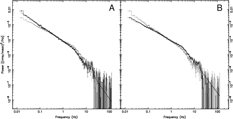
Figure 8: A comparison of the combined flare and interflare power spectra. Both (a) and (b) show the flare and interflare power spectra. In (a) the fitted flare power spectrum (black) is shown, with the interflare power spectrum (gray) for comparison, and in (b) the fitted interflare power spectrum (black) is shown, with the flare power spectrum (gray) for comparison.The solid black lines in (a) and (b) are the best fits with a broken power law and a QPO (see Table 2 for fit results). The power spectra in this figure are rms normalized, and the Poisson level was subtracted

	Flares	Interflares
$\nu_{b}$ (Hz)	2.87${}^{+0.10}_{-0.16}$	2.84${}^{+0.04}_{-0.06}$
$\alpha_{1}$	1.05$\pm$0.01	0.85$\pm$0.01
$\alpha_{2}$	2.1$\pm$0.01	1.72$\pm$0.03
0.01–1 Hz rms (%)	2.012$\pm$0.011	1.716$\pm$0.005
1–10 Hz rms (%)	1.141$\pm$0.008	1.353$\pm$0.005
QPO Frequency (Hz)	17.87$\pm$0.17	15.6${}^{+0.2}_{-0.3}$
QPO FWHM (Hz)	1.6$\pm$0.5	2.0${}^{+1.5}_{-0.8}$
QPO rms (%)	0.30$\pm$0.03	0.27${}^{+0.06}_{-0.04}$

Table 2: Power spectral properties of the combined flare and interflare observations in the 2–60 keV band.

4.2 The broad maximum and the flares

During the broad maximum of the source five flares were observed (see Figure 2). We compared the averaged power spectrum of these flares with that of the parts between the flares (hereafter ‘interflares’). For the interflare observations we took all observations between MJDs 51170 and 51237 that were neither in a flare, nor within one observation from a flare. Although their hard color (Fig. 2h) and 0.01–0.1 Hz noise (Fig. 5a) showed behavior similar to that of the flares, the observations on MJD 51220 were not included in either category, since they did not show up as a flare in the light curves and the CD.

Figure 9: The energy dependence of the 0.01–0.1 Hz (a) and 1–10 Hz (b) noise components in the flares (bullets) and interflares (diamonds). The ratios of these energy spectra are shown in (c) and (d).

Figure 10: The energy spectra of the 18 Hz QPO in the flares (a) and the 16 Hz QPO in the interflares (b). The highest energy point in (b) is an upper limit.

Figure 8 shows the 1/128–128 Hz power spectra (2–60 keV) of the combined flare observations and the combined interflare observations. For reasons explained in Section 2, we did not use a single power law to fit the noise (as we did for the individual observations). Instead, we used a broken power law, with a Lorentzian for a QPO around 15–18 Hz. The power spectral fit parameters for the flare and interflare observations are given in Table 2. Both power spectra show a clear break around 3 Hz. The noise component in the power spectrum of the flares is steeper than that in the interflare power spectrum, both below and above the break. The rms normalized power spectra of the flares and interflares cross each other around 1 Hz (see Figure 8), with the 0.01–1 Hz noise being stronger in the flares, and the 1–10 Hz noise being stronger in the interflares (see Table 2).

Figure 5a shows the strength of the 0.01–0.1 Hz noise as a function of time. When comparing this figure with Figure 2, it is evident that increases in the strength of the 0.01–0.1 Hz noise occurred at the times of the hard flares. Note that we used the 0.01–0.1 Hz noise instead of the 0.01–1 Hz noise, since the effect is more pronounced in the 0.01–0.1 Hz range. Figure 10 shows the energy dependence of the 0.01–0.1 Hz (Fig. 10a) and 1–10 Hz (Fig. 10b) noise, for both the flares (bullets) and the interflares (diamonds). From this figure it is apparent that the fractional rms energy spectrum of the 0.01–0.1 Hz noise in the flares was softer than that in the interflares (Fig. 10c), as opposed to the spectrum of the source itself, which was harder in the flares than in the interflares (Fig. 2g,h). Apart from it being stronger in the interflares below 3 keV, the 1–10 Hz noise showed (Fig. 10d) no clear spectral change between the flares and interflares. Although the detections of the noise are very significant, we note that the amplitudes are compatible with the HS observations of other sources. The large amount of data, and the relatively high count rates of XTE J1550–564 made it possible to study the HS power spectra in much higher detail than was possible in other sources before.

Apart from the difference in the noise, some of the individual power spectra during the flares also showed a QPO around 18 Hz. The only flare in which the QPO was not significantly detected was flare 3, the softest flare. Figure 8a shows the 2–60 keV power spectrum of the combined flares (including flare 3), with the QPO at a frequency of 17.87$\pm$0.17 Hz. The energy spectrum of the QPO in the flares is shown in Figure 10a. In the highest energy band (13.1–60 keV) the probable second harmonic of the QPO was detected at 35.5$\pm$2.0 Hz, with a FWHM of 10${}^{+4}_{-3}$ Hz and an rms amplitude of 4.6${}^{+1.2}_{-0.6}$%. In the two lower bands only upper limits could be determined to the rms amplitude of the harmonic: 0.17% (2–6.5 keV) and 0.8% (6.5–13.1 keV). We also searched for a QPO around 18 Hz in the combined interflare power spectra; a QPO was found at 15.6${}^{+0.2}_{-0.3}$ Hz. Its energy spectrum is shown in Figure 10b. The energy spectra of the 17.87 Hz QPO, its harmonic, and the 15.6 Hz QPO are consistent with each other.

4.3 Branch II - The Very High State

Figure 11: Four types of power spectra that were observed in the MJD 51241–51259 VHS branch (branch II). Type A on MJD 51241 and MJD 51244 (a and c), type B on MJD 51245 (b), and type C on MJD 51250 (d). Poisson level was not subtracted.

As mentioned in Section 3, the source did not return to the DBB curve after the fifth flare. On MJD 51237 (HC$\sim$0.001, SC$\sim$0.13) the source reached the position closest to the DBB curve. After that, on MJDs 51239 and 51240, it started to move away from the DBB curve, along branch II. On both these days the 18 Hz QPO was found again. On MJD 51241 the source had moved further away from the DBB curve than during the previous flares: HC$\sim$0.008, SC$\sim$0.24. The power spectrum of this observation (see Figures 11a, 12, and 20) was rather different from those seen during the HS and the flares. A broad peak around 6 Hz was found, and also a peak around 280 Hz. The presence of the 6 Hz and 280 Hz peaks, the reappearance of the hard component in the energy spectrum, and the much higher count rate compared to branch I suggest that the source had entered the VHS, as was already reported by Homan, Wijnands and van der Klis (1999). This VHS lasted from MJD 51241 until MJD 51259 (the entire branch II in the CD).

In the power spectra of nearly all the VHS observations one or more QPOs are present around 6 Hz. Although the frequency of this QPO varied between 5 and 9 Hz, for reasons of clarity this QPO will be referred to as ‘the 6 Hz’ QPO. Some observations also show a single QPO with a frequency between 100 and 300 Hz. Based on the Q-value (the QPO frequency divided by the QPO FWHM) of the 6 Hz QPO, and its harmonic structure, Wijnands, Homan and van der Klis (1999) distinguished two types of VHS power spectra: one type with a relatively broad ($Q<3$) 6 Hz QPO and sometimes a harmonic at 12 Hz (type A low-frequency QPOs; see Sec. 4.3.1), and one with a relatively narrow ($Q>6$) 6 Hz QPO, with harmonics at 3 and 12 Hz (type B low-frequency QPOs; see Sec. 4.3.2). We decided to divide type A into two subclasses; one in which the 6 Hz QPO is strong (rms $>$ 2%) and the harmonic at 12 Hz was detected (type A-I), and one in which the 6 Hz QPO was weak (rms $<$ 2%) and no harmonic was detected (type A-II). In addition to type A and B a third type, type C, was introduced by Sobczak et al. (2000b), which mainly occurred during the first part of the outburst. Its harmonic structure is similar to that of type B, but the 6 Hz QPO has a higher Q-value (Q$\gtrsim$10) and its time lag behavior is different. The only type C observation, found by Sobczak et al. (2000b), during the second part of the outburst (MJD 51250) was already classified as an odd type B observation by Wijnands, Homan and van der Klis (1999). Since this observation and the one on MJD 51254 showed odd behavior, compared to the other VHS observations, they will be discussed separately in Section 4.3.3. Figure 11 shows representative 1/128–128 Hz 2–60 keV power spectra of type A-I (Fig. 11a, MJD 51241), A-II (Fig. 11c, MJD 51244), B (Fig. 11b, MJD 51245), and C (Fig. 11d, MJD 51250).

In Table 3 the types of all observations on branch II can be found. In the remainder of this section we describe the three types of low frequency power spectra and the high frequency QPOs in more detail.

Date	Type	Frequency	FWHM	rms	rms	rms	rms
				(2–60 keV)	(2–6.5 keV)	(6.5–13.1 keV)	(13.1–60 keV)
(MJD)		(Hz)	(Hz)	(%)	(%)	(%)	(%)
51241	A-I	284$\pm$2	30${}^{+5}_{-4}$	1.06${}^{+0.14}_{-0.11}$	$<$0.9	2.8$\pm$0.3	7.7${}^{+0.9}_{-0.8}$
51242	A-I	282$\pm$3	32${}^{+9}_{-5}$	$<$1.06	$<$1.0	3.3${}^{+0.7}_{-0.5}$	$<$7
51244	A-II
51245	B	178$\pm$3	22${}^{+12}_{-7}$	1.11${}^{+0.19}_{-0.15}$	0.94${}^{+0.19}_{-0.11}$	1.5${}^{+0.3}_{-0.2}$	$<$4
51246	A-II	208${}^{+2}_{-3}$	16${}^{+13}_{-9}$	0.76$\pm$0.10	0.92${}^{+0.21}_{-0.12}$	$<$1.2	$<$3.3
51247	B	187$\pm$5	70$\pm$20	1.65${}^{+0.23}_{-0.18}$	1.54$\pm$0.19	2.51${}^{+0.25}_{-0.10}$	$<$5
51248	B
51249	B
51249	B
51250	C	102$\pm$2	18${}^{+11}_{-6}$	$<$1.3	$<$0.9	2.8$\pm$0.4	$<$3.3
51253	B
51254$<$	C1
51254$>$	B1	123$\pm$2	13$\pm$2	$<$0.8	$<$0.7	2.4$\pm$0.3	$<$3.5
51255.08	A-I
51255.12	A-I	280$\pm$3	40$\pm$10	1.22$\pm$0.19	$<$1.1	2.37$\pm$0.31	9.5$\pm$1.0
51257	A-II1
51258.1	A-I
51258.5	A-I
51258.9	A1
51259	A1

Table 3: Classification of the VHS (branch II) power spectra. For those observations where a high frequency QPO was found the frequency, FWHM, and the rms amplitudes in four energy bands are given. The frequency and FWHM are taken from the band where the QPO was most significant.
¹The type of the low frequency QPOs was uncertain.

Figure 12: The power spectrum of MJD 51241 in four energy bands. The $\sim$284 Hz QPO can be seen in the highest energy band. Poisson level was not subtracted.

4.3.1 Type A observations

On MJD 51241 (HC$\sim$0.008) the first observation in the very high state was made. The power spectrum was of type A-I, and it can be regarded as representative for the other type A-I power spectra. It is therefore the only type A-I power spectrum that will be discussed in detail in this paper. Figure 12 shows the power spectrum of MJD 51241 in four energy bands. Apart from a QPO around 6 Hz, there was some excess around 11 Hz, which in the high energy power spectra showed up as a QPO. In the 13.1–60 keV band, the 6 Hz peak had almost disappeared. The two peaks seemed to be harmonically related, but fitting them simultaneously in the 2–60 keV band gave frequencies that were not consistent with the two being harmonically related: 5.93$\pm$0.03 Hz and 10.41$\pm$0.13 Hz. However, when comparing the frequency of the lower frequency QPO in the 2–6.5 keV band (5.85$\pm$0.03 Hz) with that of the higher frequency QPO in the 13.1–60 keV band (11.52$\pm$0.19 Hz) we found a ratio of 1.97$\pm$0.03, which suggests an harmonic relation (see also Wijnands, Homan and van der Klis (1999)). The reason that the frequencies differed so much between the energy bands might be that the chosen fit function was not appropriate, or that an extra component was present between the two QPOs. The FWHM of the 5.85 Hz QPO in the 2–6.5 keV band was 2.41$\pm$0.01 Hz, and that of the 11.52 Hz QPO in the 13.1–60 keV band 7.23$\pm$0.7 Hz. Their rms amplitudes in the 2–60 keV band were 3.00$\pm$0.05% and 2.64${}^{+0.09}_{-0.08}$%. At low frequencies a noise component was present. It could be fitted with a single power law with an index of 0.90$\pm$0.03, and a strength of 1.31$\pm$0.03% rms. Figure 13 shows the photon energy spectra of the two low frequency QPOs and the noise component. The frequencies of the low frequency QPOs were not fixed, for reasons explained above. The 5.8 Hz QPO first increased in strength with energy, but above 10 keV it dropped by a factor of $\sim$2.5. Its harmonic showed a strong increase with photon energy, from $\sim$1% rms in the lowest energy bands to more than 11% rms in the highest band. The 0.01–1 Hz noise had a relatively flat energy spectrum, with strengths between 1% and 2% rms, although it became slightly weaker ($\sim$0.9%) above 10 keV. Selections were made on time, color and count rate, but no significant dependencies were found.

Figure 13: The energy spectrum of the power spectral components of the MJD 51241 (type A-I) observation. Points whose negative rms error extends to the bottom edge are upper limits.

Figure 14: The frequencies of the QPOs in the MJD 51241–51259 (VHS, branch II) power spectra as a function of hard color. Crosses depict the high frequency QPOs, circles type A-I, triangles type A-II, squares type B, and stars type C. Filled symbols represent those QPOs that according to Figure 22 can be identified with the same harmonic component. The 2.9 Hz QPO found in the MJD 51259 observations is shown as a triangle (HC$\sim$0.011), although its type (A-I to A-II) was uncertain. The QPOs of the MJD 51254 observation are plotted as type B (HC=0.195; after jump) and type C (HC=0.205; before jump), although their types were also uncertain.

The next observation, on MJD 51242, was located close to the previous observation in the CD, and its power spectrum was also very similar. Again two low frequency QPOs were found, with frequencies of 5.71$\pm$0.01 Hz (2–6.5 keV) and 11.2$\pm$0.3 Hz (13.1–60 keV), FWHM of 3.1$\pm$0.4 Hz and 8$\pm$1 Hz, and rms amplitudes (2–60 keV) of 2.53${}^{+0.11}_{-0.12}$% and 2.51${}^{+0.17}_{-0.14}$% respectively.

In the power spectrum of MJD 51244 (see Figure 11c) a QPO was found with a frequency of 8.5$\pm$0.3 Hz, a FWHM of 3.8${}^{+0.9}_{-0.7}$ Hz, and an rms amplitude of 1.34${}^{+0.13}_{-0.12}$% (2–60 keV). The QPO was considerably weaker than the 6 Hz QPOs in the two previous observations ($\sim$3% and $\sim$2.5%, 2–60 keV), and no sub- or second harmonics were found. The energy dependence of the QPO was rather steep, but in the highest band only an upper limit could be determined: 0.8$\pm$0.2% (2–6.5 keV), 2.9$\pm$0.3% (6.5–13.1 keV), and $<$3.7% (13.1–60 keV). Although the Q-value is similar to that of the previous two observations the above characteristics set this observation apart, and we therefore defined it to be of type A-II. In the CD the observation was located further along branch II, away from the DBB line and towards a stronger power law spectral component (HC$\sim$0.13).

The next type A observations occurred on MJD 51246, after a type B observation on MJD 51245 (see Sec. 4.3.2). In the CD it was located close to the MJD 51244 observation. A QPO was found at 7.72$\pm$0.13 Hz, with a FWHM of 3.1$\pm$0.4 Hz. Since the QPO was rather weak (1.20$\pm$0.06% rms) and no harmonics were found, it was classified as type A-II.

During MJDs 51247–51254 the source moved further up branch II in the CD, and the power spectra only showed type B and C QPOs (see Secs. 4.3.2 and 4.3.3). Type A QPOs reappeared on MJD 51255, when the source returned to a location in the CD close to the other type A observations (see Figure 3: HC$\sim$0.01, SC$\sim$0.2). From MJD 51255 to 51258.5 the source showed both type A-I and A–II QPOs, with similar properties as those in the beginning of the VHS. The power spectrum of MJD 51258.9 showed a broad feature around 6 Hz that had a width larger than 6 Hz, and the power spectrum of MJD 51259 showed a QPO at $\sim$3 Hz with a FWHM of $\sim$1 Hz, and a broad (FWHM$\sim$12 Hz) peak around 9 Hz. We classified these two power spectra as type A, but it was not clear of what sub-type they are; both broad peaks might have been unresolved pairs of harmonics.

Figure 14 shows the frequency of all VHS (branch II) QPOs as a function of the hard color, which is a good measure of the position along branch II, as can be seen from Figure 3. The frequencies of the broad peaks in the MJD 51258.9 and MJD 51259 power spectra are not included. Note that type A-II (triangles) observations were located both at lower and at higher hard colors with respect to the type A-I (circles) observations in Figure 14.

Figure 15: The power spectrum of MJD 51245 in four energy bands. Poisson level was not subtracted.

Frequency	FWHM	Rms Amplitude
(Hz)	(Hz)	(%)
3.15$\pm$0.03	1.3$\pm$0.1	1.54${}^{+0.06}_{-0.19}$
6.319$\pm$0.008	0.88$\pm$0.02	3.35$\pm$0.04
7.9$\pm$0.2	3.4$\pm$0.3	1.39$\pm$0.09
12.35$\pm$0.06	2.27$\pm$0.14	1.54$\pm$0.04
18.85$\pm$0.25	2.6${}^{+0.6}_{-0.5}$	0.60$\pm$0.07

Table 4: Fit values for the Gaussian peaks in the power spectrum of MJD 51245. Note that the FWHM in this case refers to the width of a Gaussian and not to that of a Lorentzian.

4.3.2 Type B observations

The first type B observation occurred on MJD 51245. The source had moved further up branch II (HC$\sim$0.016), compared to the previous (type A) observations. Figure 15 shows the power spectrum of this observation in four energy bands. A very sharp QPO was present around 6 Hz, with harmonics around 12 and 18 Hz, and a sub-harmonic around 3 Hz. There were also indications for a peak around 24 Hz, but our fits showed it was not significant. Fitting the power spectrum with a power law and Lorentzians (six in total) gave a poor result ($\chi^{2}_{red}=2.6$, $d.o.f.=230$). We tried using a power law and Gaussian functions (again six) instead, which improved the quality of the fit ($\chi^{2}_{red}=1.4$, $d.o.f.=230$, see also Wijnands, Homan and van der Klis (1999)). The two extra peaks, at $\sim$0.2 Hz and at $\sim$1.25 times the frequency of the 6 Hz QPO, were added to the fit function to account for a low frequency component, and for the shoulder of the 6 Hz QPO, respectively. The fit results (2–60 keV) for the four QPOs and the shoulder component are given in Table 4. The QPOs are not perfectly related harmonically, most likely because the fit function did not describe the data well enough. The 0.01–1 Hz noise was fitted with a single power law, with $\alpha=1.8\pm 0.1$ and an rms amplitude of 5.6${}^{+0.3}_{-0.2}$%. The photon energy spectra of the various power spectral components are shown in Figure 16. Except for the 3 Hz QPO, and the noise component, all QPOs showed a considerable increase in strength with photon energy. The 0.01–1 Hz noise only showed a weak increase, and the 3 Hz QPO behaved similar to the 6 Hz QPO in the type A-I power spectra, in that it seemed to become weaker above 10 keV. Selections were made on color, time and count rate. It was found that the harmonic at 18 Hz was more significant at low hard colors.

Figure 16: The energy spectrum of the power spectral components of the MJD 51245 (type B) observation. Points whose negative rms error extends to the bottom edge are upper limits.

Other type B power spectra were found between MJD 51247 and MJD 51253, with QPOs that were similar to those on MJD 51245. Their 6 Hz QPOs had frequencies between 5.3 Hz and 6.1 Hz, rms amplitudes between 3.3% and 3.4%, and Q-values between 6.2 and 7.3. The 3 Hz QPOs had rms amplitudes between 1% and 2.3% and showed a weak trend of an increase with hard color. The MJD 51245 observation remained the only one in which the harmonic around 18 Hz was significantly detected. Figure 14 shows the frequencies of the type B QPOs (squares) as a function of the hard color.

Figure 17: The 2–60 keV light curve (a), soft color curve (b), and hard color curve (c) of the MJD 51254 observation. The transition (around t=1100 s) can clearly be seen in the light curve. The soft color (b) does not change significantly, whereas the hard color (c) starts to decrease slowly after t=1100 s.

4.3.3 Special cases: Strong noise on MJD 51250 and the transition on MJD 51254

Although, based on the Q-value ($\sim$8) of the 6 Hz QPO and the harmonic content, the power spectrum of the MJD 51250 observation was classified as type B by Wijnands, Homan and van der Klis (1999), they also found that the time lag behavior of this observation was quite different from that of the other type B observations. Based on this time lag behavior the observation was classified as type C by Sobczak et al. (2000b), making it one of only two (see below for the second) type C observations during the second part of the outburst. More deviations from the type B power spectra were found; in addition to the power law noise (1.6$\pm$0.2 %) a strong noise component was present at 0.1–1 Hz (see Figure 11d; also Wijnands, Homan and van der Klis (1999)). This noise component, which we fitted using a zero-centered Lorentzian with a width of $\sim$3 Hz, was present in all the energy bands, with rms amplitudes of 13.1$\pm$0.3% (2–60 keV), 3.3$\pm$1.2% (2–6.5 keV), 18.6$\pm$0.5% (6.5–13.1 keV), and 28.0$\pm$0.8% (13.1–60 keV). Four low frequency QPOs were found in the 2-60 keV band at (rms amplitudes in brackets) 1.7$\pm$0.6 Hz (2.74${}^{+0.77}_{-0.45}$%), 3.35$\pm$0.03 Hz (5.8$\pm$2.0%), 6.68$\pm$0.15 Hz (6.7$\pm$0.2%), and 13.68$\pm$0.15 Hz (3.2${}^{+0.3}_{-0.2}$%). When comparing these numbers with those of the type B observations, it shows that the rms amplitudes of the 3 Hz and 6 Hz QPOs are, respectively, a factor $\sim$2.5–6 and $\sim$2 higher than in the type B observations. The QPO frequencies are shown as stars in Figure 14. In the ASM and PCA light curves the MJD 51250 observation is clearly visible as a dip (see Figures 1 and 2), with a count rate of only $\sim$5150 counts s^-1, compared to $\sim$8200 counts s^-1 on MJD 51249 and $\sim$7025 counts s^-1 on MJD 51253. This dip is strongest at low energies, causing a hardening of the spectrum a (see Figure 2).

Figure 17 shows the 2–60 keV light curve and the color curves of the MJD 51254 observation. Clearly visible is the jump in count rate that occurred around 1100 s after the start of the observation. The soft color seemed to be unaffected by this change, and though the hard color showed a small change ($\sim$10%) it was more gradual than the change in count rate. It should be noted that the observed transition is not related to the temporary gain change that was applied to the PCA later during this observation (around t=3100 s; not shown here).

Figure 18: Power spectra of the MJD 51254 observation in two energy bands, before and after the transition. Poisson level was not subtracted.

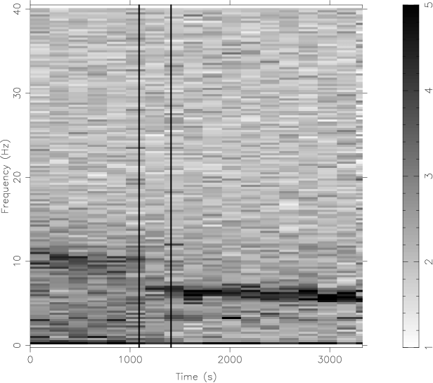
Figure 19: Dynamic power spectrum of the MJD 51254 observation in the 13.1–60 keV band. The first vertical line depicts the approximate time of transition, the second vertical represents a $\sim$300 s data gap that was only present in the high time resolution data (and therefore not visible in Figure 17). The time resolution is 3$\times$64=96 s, and the frequency resolution 32$\times$1/64=0.5 Hz .

Figure 18 shows the power spectra from before (0–1000 s) and after (1500–3000 s) the jump in the 2–60 and 13.1–60 keV bands. The 2–60 keV power spectrum before the jump showed a broad noise component around a few Hz, that was fitted with a power law with an exponential cutoff. It had a strength (1–100 Hz) of 6.7$\pm$0.1% rms, a power law index ($\alpha$) of $-$0.7$\pm$0.1, and a cutoff frequency of 3.9$\pm$0.3 Hz. In the 13.1–60 keV band the strength of this component was 12.5${}^{+0.9}_{-0.7}$% rms. In that same band we found a QPO at 9.8$\pm$0.1 Hz, with an rms amplitude of 8.6${}^{+0.6}_{-0.5}$% and a FWHM of 3.2$\pm$0.5 Hz. The post-jump 2–60 keV power spectrum showed a similar noise component as before the jump, though somewhat weaker (4.7$\pm$0.1% rms), with two QPOs superimposed on it, at 3.17$\pm$0.02 Hz and 6.14$\pm$0.03 Hz. These QPOs had rms amplitudes and FWHM of 2.3$\pm$0.1% and 0.71$\pm$0.06 Hz (3.17 Hz QPO), and 3.08$\pm$0.08% and 1.23$\pm$0.06 Hz (6.14 Hz QPO), respectively. In the post jump 2–6.5 keV power spectrum an additional QPO at 1.77$\pm$0.04 Hz was found (3.7$\sigma$) when the high count rate part was selected. Both before and after the transition power law noise was present: respectively, 3.4$\pm$0.2% rms with $\alpha=0.92\pm 0.02$ (before) and 3.8$\pm$0.1% rms with $\alpha=1.04\pm 0.03$ (after).

The fast transition in the power spectrum can be seen in Figure 19, which shows the dynamical power spectrum in the 13.1–60 keV band. The time scale for the change in the power spectrum is similar to that of the transition in the 2–60 keV light curve. It was not possible to track the QPO across the transition since it became weaker during the transition.

Wijnands, Homan and van der Klis (1999) and Sobczak et al. (2000b) classified the power spectrum after the jump as type B. Indeed, the strengths of the 3 and 6 Hz QPOs were consistent with those in the other type B observations. On the other hand, the Q-value of the 6 Hz QPO was only 5, and the 5% rms noise component under the QPOs was not seen in other type B observations. The type of the power spectrum before the jump is not clear either. The hardness of that part of the observation suggests type B or C, but the Q-value of the 9.8 Hz QPO was only $\sim$3. The strength of that QPO was lower than that of the type B and C 6 Hz QPOs in the same energy band ($\sim$11% rms), but higher than that of the type B and C 12 Hz QPOs (5–6% rms). Since the power spectrum showed a strong noise component, and the 2–60 keV count rate was lower than that of the type B part it was most likely of type C. The QPO frequencies of both parts are shown in Figure 14 (the part before [HC=0.205] as type C, the part after [HC=0.195] as type B).

The exceptional cases of low frequency QPOs presented in this section clearly demonstrate that the A, B (and C) classification. which works well for the majority of the observations, is not able to unambiguously describe all of them.The characteristics on which this classification is based (Q-value, harmonic content, time lags) show strong correlations, but deviations from the usual correlations do occur.

Figure 20: The 13.1–60 keV power spectrum of the MJD 51241 observation, showing a QPO at 284 Hz. Poisson level was not subtracted.

4.3.4 High frequency QPOs

During several observations in the VHS (branch II), QPOs were found with frequencies between 100 and 300 Hz. An example can be seen in Figure 20, which shows the 284 Hz QPO found in the power spectrum of MJD 51241. The frequencies of the high frequency QPOs ($\nu_{HF}$) are given in Table 3, and the locations in the CD of the observations in which they were found are indicated in Figure 21. Note that we only report QPOs whose single-trial significance exceeds 3$\sigma$. It can be seen from Figure 21 that $\nu_{HF}$ is related to the location in the CD. It decreased from 284 Hz to 102 Hz as the source moved up branch II, and increased again to 280 when it moved down this branch. Figure 14 more clearly shows that $\nu_{HF}$ decreased as the hard color increased. In the high energy bands, the QPOs tended to be stronger when they had a frequency around 280 Hz, as can be seen from Table 3. The Q-values of the QPOs were not related to those of the low frequency QPOs, and had values between 5.6 and 13.

We measured time lags for the $\sim$282 Hz QPO in the combined Fourier spectra of the observations on MJDs 51241, 51242, and 51255. Lags were measured between three energy bands, in the frequency range 272–292 Hz. All lags were consistent with being zero: 0.00$\pm$0.11 ms (2–6.5 keV and 6.5–13.1 keV), $-$0.08$\pm$0.13 ms (2–6.5 keV and 13.1–60 keV), and $-$0.08$\pm$0.04 ms (6.5–13.1 keV and 13.1–60 keV), where a positive number means that the photons in the second band lag those in the first one. A time lag analysis of the low frequency QPOs in the VHS (branch II) can be found in Wijnands, Homan and van der Klis (1999), Sobczak et al. (2000b), and Cui, Zhang and Chen (2000).

Figure 21: A color-color diagram showing branch II. Observations in which high frequency QPOs were found are marked with the frequency (Hz) of the QPO.

Figure 22 shows the frequency of several low frequency QPOs ($\nu_{LF}$) plotted against $\nu_{HF}$, for those observations where they were detected simultaneously. We also included the values for the high frequency QPO that was observed on branch III (represented by the diamond; see Section 4.4). The 123 Hz QPO on MJD 51254 was only found in the data taken after the count rate jump (Section 4.3.3). This data included a $\sim$600 s interval (with different PCA gain settings) that was not used for the analysis of the low frequency QPOs in Figure 14. The low frequency QPOs plotted at $\nu_{HF}=123$ Hz in Figure 22 therefore have a slightly different frequency than those of the same observation in Figure 14. Four lines could be fitted to the data points, with the first, third and fourth line having slopes that were, respectively, 0.50$\pm$0.02, 2.17$\pm$0.10, and 4.3$\pm$0.5 times the slope of the second line. This is consistent with the four lines representing the fundamental and second, fourth and eighth harmonics. Note that the four lines do not pass through the origin and cross each other around $\nu_{LF}=0$ Hz and $\nu_{HF}=75$ Hz. The only two points that were not fitted by these four lines were the sixth harmonic in the MJD 51245 observation ($\nu_{HF}$=178 Hz) and the sixteenth harmonic in MJD 51250 observation ($\nu_{HF}$=102 Hz). These components were only observed once, and therefore no fits could be made. The four lines can be used to connect the low frequency QPOs in Figure 14. For example, using the second line in Figure 22, it can be seen that the type A-I 10–12 Hz QPOs are related to the type A-II 8–9 Hz QPOs, the type B $\sim$6 Hz QPOs, the 3.1 Hz (type B?) QPO on MJD 51254, and the 1.7 Hz type C QPO on MJD 51250. The QPOs that lie on the second line in Figure 22, and those that based on similarities in the power spectrum and hard color are expected to, have been represented by the filled symbols in Figure 14. The filled symbols show that the frequency of the low frequency QPOs decreases with hard color, like that of the high frequency QPO.

Figure 22: Frequency of the low frequency QPOs as a function of the frequency of the high frequency QPOs, for those observations where they could be measured simultaneously. Similar symbols have been used as in Figure 14, based on the type of the low frequency QPOs. The four solid lines are the best linear fits to the data. The two symbols that are not fitted by a solid line are harmonics that were only observed once. They are consistent with being a 16th harmonic (highest star at 102 Hz) and a 6th harmonic (highest square at 178 Hz). Symbols on the second solid line are filled, and have been used to identify the filled symbols in Figure 14. The dashed lines represent the relations found by Psaltis, Belloni and van der Klis (1999) for the Z sources, and the dotted line the relation found by di Salvo et al. (2000a) for 4U 1728–34 (see Section 6.3). The diamond shows the values for the MJD 51270/51271 observation.

4.4 The Decay

On MJD 51260 (indicated by BEGIN in Figure 3b) the power spectrum showed no QPOs; it could be fitted with a single power law, with a strength of 0.76$\pm$0.05% rms and an index of 1.1$\pm$0.01. This weak noise, the absence of QPOs, and the relatively soft colors suggest that the source had returned to the HS.

The power spectrum of the next observation (MJD 51261) showed a noise component with a similar strength (0.56$\pm$0.07% rms), but also a QPO at 17.0${}^{+0.5}_{-0.3}$ Hz, with a FWHM of 2.5${}^{+1.9}_{-1.1}$ and a rms amplitude of 1.02${}^{+0.20}_{-0.16}$%. Based on the hardness at which this QPO is found, its frequency, and its FWHM, it may be related to the 15.6/17.9 Hz QPO that was found in the flare/interflare observations during MJD 51170–51237 (see section 4.1). In the next few observations (MJD 51263–51267) no QPO around 17 Hz was found, and the power spectra could be fitted with single power laws, with strengths between 0.4% and 1.2% rms, typical for HS.

On MJD 51269 the source had started to move up branch III. Two QPOs were found in the power spectrum of that observation: at 4.54$\pm$0.15 Hz (1.7$\pm$0.2% rms, FWHM=1.5${}^{+0.5}_{-0.4}$ Hz) and 9.6$\pm$0.6 Hz (2.0${}^{+0.4}_{-0.3}$% rms, FWHM=4.5${}^{+2.4}_{-1.5}$ Hz). The noise at low frequencies was fitted with a single power law, with a strength of 1.32$\pm$0.07% rms and an index of 0.8$\pm$0.1. Based on their Q-values, the QPOs are either of type A-I or A-II; the strength of the QPOs (and their frequency) suggests type A-II, whereas the detection of an harmonic suggest type A-I (see section 4.3.1).

The next two observations (MJDs 51270 and 51271) were located near the top of branch III. Their power spectra were very similar. The MJD 51270 power spectrum showed a QPO at 8.9$\pm$0.1 Hz (1.8${}^{+0.2}_{-0.1}$% rms, FWHM=2.1${}^{+0.5}_{-0.3}$ Hz) and a broad peak around 2 Hz that was fitted with a Gaussian at 1.8$\pm$0.1 Hz (3.2$\pm$0.2% rms, FWHM=2.9$\pm$0.4 Hz) plus an exponentially cutoff power law (4.4$\pm$0.3% rms, $\alpha=-$1.6$\pm$0.6, $\nu_{cutoff}=4\pm$1 Hz). The power spectrum of MJD 51271 showed a QPO at 9.05$\pm$0.12 Hz (1.8${}^{+0.3}_{-0.2}$% rms, FWHM=1.4${}^{+0.5}_{-0.4}$ Hz) and a broad peak around 2 Hz that was fitted with a Gaussian at 1.7$\pm$0.3 Hz (3.8${}^{+0.4}_{-0.3}$% rms, FWHM=3.74$\pm$0.5 Hz) plus an exponentially cutoff power law (4.5$\pm$0.4% rms, $\alpha=-$2.3$\pm$1.0, $\nu_{cutoff}=3\pm$1 Hz). The combined 1/128–128 Hz power spectrum of the two observations is shown in Figure 23b. The strength of the 0.01–1 Hz noise, which was fitted with a power law, was $\sim$1.5% rms, but it should be noted that some of the power in the 0.01–1 Hz range was absorbed by the Gaussian and the exponentially cutoff power law. The two $\sim$9 Hz QPOs had relatively high Q-values (4.2 and 6.5), which suggests that they were of type B; this seems to be confirmed by the shape of the power spectra at higher energies; Figure 24 shows the 6.5–60 keV power spectrum of MJD 51271, which could be fitted with a power law and QPOs at 3.1$\pm$0.1 Hz, 5.7$\pm$0.2 Hz, 9.0$\pm$0.1 Hz, and 12.5$\pm$1.0 Hz. This is reminiscent of the type B QPO found on branch II, and the IS power spectrum shown in Figure 7. In the combined 2–60 keV power spectrum of the two observations a QPO at 251$\pm$3 Hz was found. It had an rms amplitude of 2.21$\pm$0.15% and a FWHM of 42$\pm$6 Hz. Its location in Figure 22 is shown by a diamond. Although the frequency of the QPO lies in the $\nu_{HF}$ range found on branch II, the count rate at which is was found was considerably lower ($\sim$1350 counts s^-1 compared to 4700–8300 counts s^-1 on branch II).

Figure 23: Four power spectra during the decay: (a) bottom of branch III (MJDs 51269 and 51273), (b) top of branch III (MJDs 51270 and 51271), (c) bottom of branch IV, and (d) top of branch IV. Poisson level was not subtracted.

Figure 24: The 6.5–60 keV power spectrum of MJD 51271, showing similar structure as found in the type B power spectra. The solid line shows the best fit with four QPOs and a power law. Poisson level was not subtracted.

The power spectrum of the next observation (MJD 51273), which in the CD was located close to the MJD 51269 observation, showed a QPO at 4.52$\pm$0.13 with an rms amplitude of 1.2$\pm$0.02% and a FWHM of 1.1${}^{+0.5}_{-0.3}$ Hz. The QPO is most likely of type A, based on its strength and lack of harmonic structure. The low frequency noise had a strength of 1.20$\pm$0.05% rms. The combined power spectrum of MJDs 51269 and 51273 is shown in Figure 23a.

The observation on MJD 51274 showed no QPOs, and the 0.01–1 Hz noise had an rms amplitude of less than 0.4%. During MJD 51274–51280 (HC$\sim$0.007, SC$\sim$0.13) the source showed similar power spectra that, when combined, were fitted with a single power law with a strength 0.90$\pm$0.09% rms and an index of 1.0$\pm$0.2, which is typical for the HS.

Between MJD 51283 and MJD 51298 XTE J1550–564 traced out branch IV in the CD. At the top of the branch (SC$>$0.35) the power spectra showed a QPO and a peaked noise component. These were not found at the bottom of the branch (SC$<$0.35). The combined power spectrum of the bottom of branch IV (Fig. 23c) was fitted with a power law with an rms amplitude of 2.4$\pm$0.2% and an index of 0.7$\pm$0.1. In the combined power spectrum of the top of branch IV (Fig. 23d) a QPO was found at 11.3$\pm$0.5 Hz, with an rms amplitude of 4.1${}^{+0.7}_{-0.5}$% and a FWHM of 2.9${}^{+1.1}_{-0.8}$ Hz. A peaked noise component was present below 10 Hz. It was fitted by a Lorentzian with a frequency of 3.0$\pm$0.3 Hz, an rms amplitude of 10.1${}^{+0.9}_{-0.8}$%, and a FWHM of 5.7$\pm$0.9 Hz. The 0.01–1 Hz noise was fitted with a power law that had a strength of 2.8$\pm$0.4% and an index of 0.3$\pm$0.1.

Both branch III and IV showed behavior that was similar to that seen in the VHS (branch II). Since the count rates were lower than on the branch II, these branches were probably IS (at least, when QPOs were seen).

Figure 25: Combined power spectrum of the last six observations during the low state (MJD 51307–51318). The solid line is the best fit with a broken power law. The Poisson level was subtracted.

Between MJD 51299 and MJD 51318 branch V was traced out in the CD. It reached much harder colors than before, and the movement up the branch was accompanied by a considerable increase in the strength of the low frequency noise, as can be seen from Figure 5. There was a clear difference between the power spectra at the top and bottom of the branch. The combined MJD 51299–51306 (bottom part of branch V, SC$<$0.6) power spectrum was fitted with a power law with an rms amplitude of 8.9$\pm$1.0% and an index of 0.7$\pm$0.1. A single power law yielded a poor $\chi^{2}_{red}$ (3.2 for d.o.f.=67) for the combined MJD 51307–51318 (top of branch V, SC$>$0.6) power spectrum, and a broken power law was used instead (see Figure 25). Its rms amplitude was 15.9$\pm$0.3%, with $\nu_{break}=0.9\pm 0.1$ Hz, $\alpha_{1}=0.33\pm 0.04$, and $\alpha_{2}=1.2\pm 0.1$ ($\chi^{2}_{red}=1.1$ for d.o.f.=67). The strength and shape of the noise, and the spectral hardness suggests that the bottom of branch V the source was in the IS, and that at the top of branch V the source was in the LS.

5 Radio Observation

On 1999 March 11 (MJD 51248) we observed the radio counterpart of XTE J1550–564 (Campbell-Wilson et al., 1998) with the Australia Telescope compact array (ATCA), in a high-resolution 6 km configuration. Observations were made simultaneously at 6.3 and 3.5 cm, and at 21.7 and 12.7 cm, in order to obtain broad band spectral coverage. The observations were interleaved with those of a nearby reference source B1554-64, for phase calibration every 25 min. The source was clearly detected at all four wavelengths; the mean flux densities at 21.7, 12.7, 6.3 & 3.5 cm were, respectively, 5.1, 3.0, 2.8, and 1.9 mJy (errors $\sim$10%). The four flux densities were fitted with a power law corresponding to a spectral index ($\alpha=\Delta logS_{\nu}/\Delta log\nu$) of $-$0.53$\pm$0.12. The location of the MJD 51248 RXTE observation is indicated with by ‘ATCA’ in Figure 3.

6 Discussion

In this section we present a discussion of our results. We start by briefly summarizing the results. After that the source states and power spectra are discussed.

6.1 Summary of Results

In the period of 1998 November 22 to 1999 May 20 XTE J1550–564 showed a wide variety of behavior. To organize the different phenomena and relate them to each other, it is useful to compare the rapid time variability and the energy spectra. An initial division of the observations can be made based on the strength of the broad band (1/128–128 Hz) power, which is shown in Figure 5b. It can be seen that the source alternated between states with low power (a few percent rms) and states with high power (more than a few percent). When comparing this figure with Figure 2 it is obvious that observations with high power were mainly found when the spectrum was hard. These spectrally hard states appeared as branches (I–V) in the color-color (Fig. 3) and hardness-intensity (Fig. 4) diagrams. From the hardness-intensity diagram it is apparent that the hard branches occurred at five distinct count rate levels, and that they were separated by periods that were spectrally soft(er); in the color-color diagram the hard branches lay more or less parallel to the power law curve. The power spectra on the five hard branches often showed QPOs, and in some cases also strong peaked and/or band limited noise (Fig. 11). These properties classify the observations on the branches as VHS, IS, or LS. The power spectra that were not on the hard branches showed noise with strength of a few percent rms and, when combined, a weak QPO around 17 Hz (Fig. 8). These observations can be classified as HS; in the color-color diagram they lay close to the disk blackbody curve. When the source moved up a hard branch the low frequency noise changed from a weak power law to strong band-limited. On branch II this change was accompanied by the QPOs changing from the broad type A, to the narrow types B and C (Fig. 14). On branches II and III we also found high frequency QPOs in the 102–284 Hz range. Their frequencies were anti-correlated with the hardness of the energy spectrum (Fig. 14), and correlated with the frequency of the type A, B, and C low frequency QPOs (Fig. 22).

6.2 Source States

In recent years the picture of black hole behavior that emerged from observations was consistent with a one-dimensional scheme, in which four canonical source states were linked by one parameter, usually taken to be the mass accretion rate (see, e.g. Esin, McClintock and Narayan (1997) and Esin et al. (1998) for recent elaborations on this view). In the context of two-component spectral models, often interpreted in terms of emission from an accretion disk and a hot comptonizing medium, this implies that both components contribute to the energy spectrum and power spectrum in amounts that depend strictly on this parameter; if both components were to vary independently, the description of the phenomenology would have to be at least two-dimensional. XTE J1550–564 seems to provide evidence for such two-dimensional behavior. Although the source was observed in all four canonical states, their occurrence was more complex than expected on the basis of a simple relation with the mass accretion rate.

We start by discussing the relation between the source states and the position of the source in the CD and HID (see Figures 3 and 4). The motion of the source through the CD was along branches. One branch (hereafter the soft branch) lay parallel to the DBB curve in the CD, and quite close to it (Fig 3a). Whenever XTE J1550–564 was on or close to this branch (e.g. flares 1-5), it could be classified as being in the HS: it showed soft energy spectra, and the (power law-like) low frequency noise had a strength of only a few percent rms. All the other branches (hereafter hard branches) lay approximately parallel to the power law curve in the CD. In time, these hard branches were traced out one after the other, and all but the last two were clearly separated from each other by intervals that showed HS behavior. When the source was on a hard branch it was in the VHS, IS or LS: the energy spectrum was hard, and the power spectrum showed QPOs and/or strong noise. The hard branches were similar to each other in that the shape of the noise changed from power law like to band limited as the source moved up such a branch (i.e. when it became harder). When the source was on a hard branch still relatively close to the soft branch it would, based on the energy and power spectrum, usually be classified as being in the canonical HS - only further up the hard branches full-fledged VHS, IS and LS behaviour emerged. Canonical LS (variability) behavior was only found at the top of branch V, the branch that reached the hardest colors.

Although the observations on hard branches I, III, and IV were classified as IS, and those on hard branch II as VHS, they had in fact very similar properties, the only difference being the count rate at which they were observed. This was already found for the IS and VHS in other sources, e.g., GS 1124–68 and GX 339-4 (Belloni et al., 1997; Méndez and van der Klis, 1997). We therefore regard the VHS as an instance of the IS, but just the one that happens to be the brightest.

The behavior on the hard branches that were traced out before our observations, during the first part of the outburst, was similar to that during our observations (Remillard et al., 1999a; Cui, et al., 1999). During the first part of the outburst LS behavior (strong band limited noise with a break around 0.1 Hz) was observed only when the hardness was similar to that at the top of branch V (at the start of the outburst, when the count rate was $\sim$100 times as high as on branch V). Moreover, the source evolved from LS to the HS via a VHS (or IS as we shall henceforth call it), clearly showing the same ordering of states (as a function hardness) as during our observations.

The above shows that as the hardness increased the source evolved from the HS via the IS, to the LS; the hard branches therefore corresponded to HS$\leftrightarrow$IS$\leftrightarrow$LS transitions, or at least attempts to, since not every branch reached the LS and the source did not always return completely to the HS. Similar conclusions were also drawn by Rutledge et al. (1999), on the basis of a comparative study of 10 black hole candidates. They found that the VHS and IS were spectrally intermediate to the HS and LS, and also that as the hardness increases the noise switches from HS-like to LS-like. They also concluded that transitions between the HS and LS could take place at luminosities/count rates both above and below that of the HS. In our observations transitions between HS and IS were found at around 8000, 1200, 600, and 200 counts s^-1 (see Fig. 4); transitions between IS and LS were found at around 40 (Fig. 4) and 4000 counts s^-1 (during the first part of the outburst). Moreover we observed HS behavior at all count rate between 200 and 10000 count s^-1. All this argues against a one-dimensional description of the state transitions as a function of the mass accretion rate.

The observations of XTE J1550–564 contradict the old picture of black hole states, in which hard states are only found at the highest and lowest count rates. XTE J1550–564 clearly shows that hard states can be observed at any count rate level. However, some remarks should be made. All the hard states (I–V) were observed during the decay of the source (I during the decay of the first part of the outburst, II–V during the decay of the second part). Also, the intervals between branches II–IV, although they could be classified as HS, had significantly harder spectra than the HS observations during the rise, which were extremely soft. This suggests that the conditions for the presence of the hard spectral component are more favorable during the decay or phases of low count rate. This is supported by the fact that all small flares (1–5) were observed at count rates higher than that of the hard branches. The fact that these flares did not develop into real transitions suggests that the conditions for transitions and development of the hard spectral component are less favorable at the highest count rates. Also, it can be argued that the only LS that was observed during our observations was found at the lowest count rates at the end of the outburst, as expected in the canonical picture of black hole states. On the other hand, a LS was also found during the first part of the outburst when the count rate was at least a factor 100 higher than during the LS at the end of the outburst, clearly showing that LS is not only found at the lowest count rates.

Figure 26: A diagram of the two-dimensional behavior of XTE J1550–564 during the second part of its 1998/1999 outburst. In the color-color and hardness-intensity rate diagrams the source traced out a comb-like structure, with the spectrally soft state (HS) being the regions on and near the spine, and the HS$\leftrightarrow$IS(VHS)$\leftrightarrow$LS transitions being the teeth. The comb-like structure in the CD and HID is caused by three effects. First, the disk and power law luminosity change to a large extent independently. Second, the power law luminosity can be negligible for times comparable to the time scale on which the disk luminosity changes. Third, the time scale on which the power law luminosity changes, when it is not negligible, is short compared to that of the disk luminosity changes. As the relative contribution of the power law component increases, the low frequency noise changes from HS-like (weak power law) to LS-like (strong band limited). In this scheme it is possible to have a soft state (HS) at a higher disk luminosity than a the brightest IS (VHS). Although the structure traced out by XTE J1550–564 was comb-like, similar two-dimensional behavior of other black holes may lead to different structures.

Based on the CD, HID, and power spectral fits one gets the impression that the behavior of XTE J1550–564 is two-dimensional, i.e. at least two (observable) parameters are needed two describe the appearance of the source and to account for the occurrence of the different states. Phenomenologically, the two parameters describing this two-dimensional behavior are the count rate and the spectral hardness. A schematic representation of the behavior of XTE J1550–564 in terms of these parameters is shown in Figure 26. It shows that the states are arranged in a comb-like topology, with the soft (HS) branch being the spine, and the HS$\leftrightarrow$IS$\leftrightarrow$LS transitions being represented by the teeth. Note that the parameter on the vertical axis is the logarithm of the count rate, and that we decided to show the hard branches as horizontal lines; for reasons of clarity we did not depict the exact movement of the source through the diagram. We also included the location of the flares, which occurred at count rates higher than that of the brightest hard branch.

The most important aspect of XTE J1550–564 is probably the fact that two observable parameters (count rate and hardness) varied too a large extent independently from each other. This suggests that at least two physical parameters underlie this behavior, since this complex behavior is hard to explain within a framework where the appearance of the source is determined by a only single physical parameter (e.g. only mass accretion rate). Physically the two underlying parameters might for example be the mass accretion rate through the disk (roughly increasing with count rate, at least in the HS) and the size of a Comptonizing medium (increasing with spectral hardness). In that case the state of the source is determined by the (relative) size of the Comptonizing medium, with it being small or absent in the HS and growing in size towards the LS. The fact that we see increases in the spectral hardness at many count rate levels suggests that the size of this medium, and therefore also the state of the source, is to a large degree not determined by the accretion rate through the disk. We note that the inner disc radius as derived from variability properties (i.e. QPO frequencies, see Section 6.3.2) correlates well with hardness, suggesting that the Comptonizing medium grows as the inner disk edge moves out. The two physical parameters do not necessarily vary completely independently from each other. For instance, changes in one parameter may be triggered by changes in the other, and certain values of one parameter may restrict the value of the other parameter (e.g. in between the hard branches XTE J1550–564 seemed to become slightly harder towards lower count rates (Fig. 4)).

While previous authors, inspired by the description of black hole spectra in terms of two components, have also discussed black hole phenomenology in terms of two-dimensional diagrams (Miyamoto et al., 1994; Nowak, 1995), the overall picture has in our view been considerably clarified by the clues provided by XTE J1550–564 described in this paper. The basic phenomenology seems to be one where the hard and soft component can vary to a large extent independently from each other. The HS is the name we have given in the past to all cases where the hard component is weak compared to the soft component, and the IS/VHS and LS are unified into cases where the hard component is, respectively, comparable to or dominating the soft component. The difference between the VHS and IS is reduced to a difference in the luminosity of the soft component at which they occur, and the difference between IS/VHS and LS is caused by differences in the relative contributions of the soft and hard components.

This two-dimensional interpretation might very well be applicable to all black hole candidates showing the canonical states. The often observed order of states (VHS$\rightarrow$HS$\rightarrow$IS$\rightarrow$LS) is still consistent with the diagram drawn Figure 26. The fact that black hole state behavior often seems one-dimensional can be explained by considering how the behavior of XTE J1550–564 would have appeared if the data were of lower quality, the source sampling was more infrequent, its distance was larger, and if it had different characteristic time scales for variations in the soft and hard component. Much of its subtle behavior would have been missed or may have been misinterpreted. It is mainly thanks to the combination of source brightness, the quality of the RXTE/PCA data, and the excellent source sampling that we clearly see the two-dimensional nature of its behavior. Since the observations of XTE J1550–564 strongly suggest that mass accretion rate through the disk and state are decoupled, it would be possible to see transients that remain in the same state during a whole outburst. Moreover, one could also see state transitions in sources with a more or less constant mass accretion rate. Suggestions of such behavior have been seen in, respectively, GS 2023+338 (Sunyaev et al., 1991; Terada et al., 1992; Miyamoto et al., 1992) and Cyg X-1 (Zhang et al. (1997), however see Frontera et al. (2000)).

The radio brightness of XTE J1550–564 during the MJD 51248 ATCA observations indicates that an outflow event was going on or had recently occurred. The spectral index suggests that the radio source was optically thin, and observed during the decay of such an outflow event. This event might be associated with the state change on MJD 51237/51239 (the onset of branch II). Although XTE J1550–564 was observed in radio only once (on branch II), observations of other black hole candidates (Fender et al., 1999, 2000) suggest that radio emission is associated with spectrally hard states. The hard branches may therefore correspond to changes in the accretion flow geometry, where an inflow (HS) is gradually accompanied by (or changing into) an outflow (LS). Jet-like outflow models have already been proposed for the VHS in GX 339–4 by Miyamoto and Kitamoto (1991).

6.3 Power spectra

Although not always observable in individual observations, QPOs were found on all branches, except for the last one. Several types were found: 1–18 Hz QPOs on the hard branches (type A, B, and C), 15–18 Hz (plus an harmonic) on the soft/HS branch and in the flares, and 100–285 Hz QPOs on the two brightest hard branches.

6.3.1 High frequency QPOs

High frequency QPOs in black hole candidates are a relatively new phenomenon. Previous to XTE J1550–564, they were found in GRS 1915+105 (Morgan, Remillard and Greiner, 1997, 67 Hz) and in GRO J1655-40 (Remillard et al., 1999b, 300 Hz). Remillard et al. (1999a) found high frequency QPOs in XTE J1550–564 in the 161–238 Hz range, during the first part of the outburst. With the observations of the second part of the outburst this range has been expanded to 100–285 Hz. It is obvious that the frequency of the high frequency QPOs in XTE J1550–564 can not be explained by models that predict an approximately constant frequency, e.g. orbital motion at the innermost stable orbit (Morgan, Remillard and Greiner, 1997), Lense-Thirring precession at the innermost stable orbit (Cui, Zhang and Chen, 1998), or trapped-mode disk oscillations (Nowak et al., 1997).

The high frequency QPO was found on two branches; between 100 and 285 Hz on branch II, and at 251 Hz on branch III. The count rates at which it was observed, were much lower on branch III ($\sim$1350 counts s^-1) than on branch II ($\sim$4700-8300 counts s^-1), which shows that the QPO frequency does not strongly depend on the count rate. A similar effect is also seen for the high frequency QPOs in some neutron star X-ray binaries (Méndez et al., 1999; Ford et al., 2000), where the frequency varies along parallel branches in a frequency–count rate diagram. A certain frequency can therefore be observed at different count rate levels, and a range of frequencies can be found within a relatively small range of count rates. This suggests that if the QPO frequency is related to a certain (variable) radius, this radius varies almost independently from the count rate (and probably mass accretion rate; van der Klis (2000)). Similar two-dimensional behavior as discussed in Section 6.2 may therefore also be present in some of the neutron star sources.

An obvious question to ask is, whether the high frequency QPOs in black hole candidates have the same origin as the kiloHertz QPOs that are observed in the neutron star sources (see van der Klis (2000) for a review). Of course, since the QPOs in the neutron star sources are often observed in pairs, only one (if any) of those two QPOs can have the same origin as the QPOs in black hole sources, which until now have always appeared as single peaks. It is, however, not clear which of the two QPOs that would be; both the lower and upper kHz QPO have Q-values and the rms energy spectra that are consistent with those of the QPO in XTE J1550–564. The frequency ranges in which the high frequency QPOs are observed are 102–284 Hz for the QPO in XTE J1550-564, and 200–1070 Hz for the lower kHz QPO, and 325–1330 for the upper kHz QPO in the neutron stars. Here we combined the kHz QPO data for all neutron star sources in van der Klis (2000). Although the lower and upper kHz QPOs cover a frequency range of a factor of 5.4 and 4.1, respectively, the values for individual neutron star sources are more like that found for XTE J1550–564 ($\sim$2.8).

Although the high frequency QPO in XTE J1550–564 has parameters that are consistent with those of both the lower and upper kHz QPO (within a simple orbital frequency model), a major difference between XTE J1550–564 and the neutron star sources is the fact that the latter often show two high frequency QPOs. However, this could be explained if one of the two kHz QPOs in the neutron star sources is due to a mechanism that requires the presence of a solid surface.

6.3.2 Low frequency QPOs

On all the hard branches, except branch V, QPOs were found with frequencies between 1 and 18 Hz. Due to the low count rates the quality of the power spectra on branch V was poor, and the presence of QPOs could therefore not be ruled out. The frequencies of the QPOs were not constant, as can be seen from Figure 14 (showing the QPOs found on branch II), but it is not immediately clear from that figure how the frequency of the low frequency QPOs ($\nu_{LF}$) depended on the hard color (which is a good measure of the distance along the branch). Although the figure is suggestive of a positive correlation, especially for HC$<$0.015, the behavior of the low frequency QPOs during the rise of the first part of the outburst of XTE J1550–564 (anti-correlation with hardness; Cui, et al. (1999)) and the correlation found between the low and high frequency QPOs (see below, and Figure 22) lead us to believe that hard color and frequency were anti-correlated, and that the frequencies of both the high and low frequency QPOs decreased as the source moved up branch II. This contradicts the switch from a correlation into anti-correlation when the hard color passes a certain value, that was reported by Rutledge et al. (1999) for other black hole candidates. We want to stress again that the fact that several harmonics were present and that not always the same harmonic was the strongest one, can easily lead to confusion. On the other hard branches not enough QPOs were observed to confirm the anti-correlation with hardness.

It was usually the QPO that happened to be located between 5 and 8 Hz that was the strongest in the 2–60 keV power spectra of branch II, even though it could be identified with different harmonic components (as can be seen from Figures 14 and 22). Perhaps variations within that frequency range are less prone to damping than outside, or a resonance occurs. The shoulder component that was present at a frequency of 1.25 times that of the 5–8 Hz type B QPOs, has been found before in QPOs in other black hole candidates like GS 1124–68 and GX 339–4 (Belloni et al., 1997), but recently also in the 20-50 Hz QPOs in the neutron star system GX 340+0 (Jonker et al., 2000).

Figures 14 and 22 seem to indicate that the low frequency QPOs evolve from type A via type B into type C, and vice versa. On branch II the type A QPOs were located at the bottom of the branch, and the those of type B and C further along it. This was also seen on branch III for type A and B (Figs. 23 and 24), and to certain extent also on branch I, where indications for type B QPOs were found at a similar hardness as where they were found on branch II (Fig. 7). No direct transitions between type A and B were seen, so it is not known whether such transitions are smooth or abrupt. In the MJD 51254 observation a jump in the count rate was accompanied by a change in the power spectrum that may have been a transition from type C to B. This suggests that the transitions between the different types are quite sudden. Apart from the difference in spectral hardness at which type A and B occurred, it is clear that there are at least two other fundamental differences between the two types. First there is the difference in the Q-value, which is higher in type B. This might also explain why more harmonics are detected in the type B power spectra, since narrower features are easier to identify. Second, there is the difference in time lag spectra (Wijnands, Homan and van der Klis, 1999), which can not be reconciled even when one compares the time lags of similar harmonics (i.e., the type A-I 12 Hz QPO and the type B 6 Hz QPO, which in our view are supposed to be the same harmonic, still have the opposite signs for their time lags). As mentioned already in Section 4.3 the type A QPOs were divided in two types, A-I and A-II. Figure 14 shows that type A-II QPOs (triangles) were found both at higher and lower hardness than type A-I (circles). The A-II subtype should therefore be regarded as a collective rather than a real type. The two filled triangles (HC$\sim$0.012) can be identified with second harmonics and are for that reason different from the A-I observations, where the fundamental was the dominant harmonic. The nature of the two observations represented by the open triangles in Figure 14 remains uncertain; their frequency is lower than expected on the basis of their hardness and in one case an addiational broad bump was observed in the power spectrum.

We found that the frequencies of the high frequency QPOs and low frequency QPOs that were detected simultaneously are well correlated (Fig. 22); it is mainly on the basis of this that we conclude that the different types (A, B, and C) of low frequency QPOs have the same origin. Similar correlations have also been found for the low and high frequency QPOs in a number of neutron star source (e.g. van der Klis et al. (1996); van der Klis, Wijnands, Horne and Chen (1997); Wijnands et al. (1997); Jonker et al. (1998); Ford and van der Klis (1998); Psaltis et al. (1999); Markwardt, Strohmayer and Swank (1999)) and in neutron star and black hole sources for QPOs and broad noise components (Psaltis, Belloni and van der Klis, 1999). The main correlation that was found for the neutron star and black hole sources extended over a frequency range of 0.1–1200 Hz, and was consistent with the relation $\nu_{LF}=(42\pm 3)(\nu_{HF}/500\,Hz)^{0.95\pm 0.16}$, that was found in the neutron star Z sources (Psaltis et al., 1999; Psaltis, Belloni and van der Klis, 1999). A second correlation was present in Figure 2 of Psaltis, Belloni and van der Klis (1999) that was fitted with $\nu_{LF}=2.09\times 10^{-3}(\nu_{HF})^{1.46}$ by di Salvo et al. (2000a) for data of 4U 1728–34. Both relations are plotted in Figure 22 (dashed and dotted lines, respectively), and are apparently not consistent with the data of XTE J1550–564.

The fact that the data in Figure 22 are well fitted with four linear relations that do not pass through the origin excludes models in which $\nu_{LF}$ and $\nu_{HF}$ are related by a simple power law expression. The four linear fits to the data in Figure 22 cross each other at $\nu_{LF}\sim$0 Hz and $\nu_{HF}\sim$ 75 Hz. It is not clear what the nature of this $\sim$75 Hz frequency in a black hole system could be.

Low frequency QPOs were also found on the soft branch (15.6 Hz) and in the high state flares (17.9 Hz). They were much weaker than the low frequency QPOs found on the hard branches and had a rather high Q-value ($\sim$10). Their frequency was apparently correlated with hard color (assuming that we observed the same harmonical component), unlike that of the hard branch QPOs. The above suggests that the 15.6 Hz and 17.9 Hz QPOs may have a different origin than the type A, B and C QPOs, and it may also explain why the only 18 Hz QPO (MJD 51239) reported by Sobczak et al. (2000a) did not follow the relation between QPO properties and the spectral parameters seen on the hard branches. On the other hand, there some clues that do suggest a relation with the type A, B, and C QPOs: when their values would be plotted in Figure 14 they would lie close to the extrapolation of a line through the filled symbols. Moreover, the 15.6 Hz and the 17.9 Hz QPO both fall on the empirical relation found by Wijnands and van der Klis (1999) for the low frequency QPO and break frequency found in many types of X-ray binaries, including black holes. Hence, it is not clear whether these QPO really have a different origin than the A, B, and C type QPOs, or that they only have appear to be different because the hard spectral component is so much weaker. The properties of the 16–18 Hz QPO are in fact remarkably similar to those of the 14–23 Hz QPO in GRO J1655–564, studied by Sobczak et al. (2000a); the similarity extends to the frequency at which they are found, their amplitude, and their relation with the disk spectral parameters. Note the apparent switch from a correlation of QPO frequency with hardness (15.6 Hz and 17.9 Hz QPOs) to an anticorrelation (A, B and C types) is probably not related the one reported by Rutledge et al. (1999, see above). They did not find QPOs in such spectrally soft states, and the frequencies of the 15.6/17.9 Hz QPOs are still well above that of most A, B, and C type QPOs.

The range over which the fundamental of the low frequency QPOs is observed in XTE J1550–564 is 0.1 Hz to 6 Hz (which includes the QPOs reported by Cui, Zhang and Chen (1998), but not the 16–18 Hz QPOs discussed in the previous paragraph). Using the expression for the lowest line in Figure 22, $\nu_{HF}=38.1(\nu_{LF}+1.61)$, and assuming that the high frequency QPO is due to orbital motion at inner disc radius ($R_{in}$), $\nu_{HF}\propto R_{in}^{2/3}$, one can estimate the corresponding changes in the inner disc radius. For the low frequency QPO changing from 0.1 to 6 Hz we find a decrease in $R_{in}$ by a factor 2.6, which is comparable to what was found by di Matteo and Psaltis (1999) for other black hole systems. However, their relation between $R_{in}$ and $\nu_{LF}$ was based on the empirical relation between $\nu_{LF}$ and $\nu_{HF}$ found for neutron star sources by Psaltis, Belloni and van der Klis (1999). Using the relation of di Matteo and Psaltis (1999) we find a decrease in $R_{in}$ by factor $\sim$4.2. Both numbers suggest that the inner radius changes are rather small when a black hole changes from a hard (where the 0.1 Hz QPO was observed) to a much softer state (where the 6 Hz QPO was observed). It should be noted that these changes may in fact be somewhat larger if the 15.6/17.9 Hz QPO turns out to be related to the A, B, and C type QPOs, and/or if the lowest peak in the Cui, Zhang and Chen (1998) power spectra is not the fundamental, but a higher harmonic.

There are two types of low frequency QPOs in the neutron star Z sources (Hasinger and van der Klis, 1989) that may be compared with the low frequency QPOs in XTE J1550–564 (and other black hole candidates): these are the horizontal branch QPOs (HBO) and the normal branch QPOs (NBO) (see van der Klis (1995b) for a review). Similar QPOs have also been found in a number of neutron star atoll sources. Of the two QPO types in Z sources it is the HBO that bears most resemblance to the QPOs in XTE J1550–564. Unlike NBOs, HBOs have a strong harmonic content; e.g., in GX 340+0 the HBOs could be fitted with three harmonically related peaks (1st, 2nd and 4th) plus a shoulder component for the second harmonic (Jonker et al., 2000), similar to the type B QPOs in XTE J1550–564. HBOs are found in the 15–60 Hz range, and their frequency changes smoothly; NBOs are found in the 6–20 Hz range, but their frequency changes are strongly related to sudden spectral/state changes. Although the 6–20 Hz range of the NBOs is closer to the values we found for the low frequency QPOs in XTE J1550–564, it should be noted that if one scales the frequency of those low frequency QPOs with a factor $\sim$5 (which is maximum $\nu_{upper}$ in the neutron star sources divided by the maximum $\nu_{HF}$ in XTE J1550–564), one gets values that are similar to those found for the HBO. Another indication that the QPOs in XTE J1550–564 are related to the HBOs (at least to the HBOs in the Z source GX 17+2 (di Salvo et al., 2000b; Homan et al., 2001) ) is the fact that they are both observed when a hard power law tail is present in the energy spectrum, and that both show an anti-correlation between their frequency and the strength of this high energy component. Finally we note that the HBO in Z sources is accompanied by a low frequency noise component that becomes stronger when the HBO frequency decreases, which is similar to what is observed in XTE J1550–564, where a strong noise component develops when the QPO frequency drops (see also figures in Cui, et al. (1999) and Remillard et al. (1999a)).

When comparing the properties of the 0.01–0.1 Hz noise in the high state flares with those in between the flares, we find that in the flares the noise was stronger, but had a softer fractional rms spectrum, whereas the overall X-ray spectrum of the source was harder. Though this might at first appear remarkable, it is in perfect agreement with the assumption that the extra noise is associated with the hard power law component. A hard spectral component, with associated noise that remains a constant fraction of it, in combination with a soft spectral component that remains unchanged, will lead to a softer fractional spectral dependence of the noise when the hard component increases.

The transition observed on MJD 51254 showed many similarities to the “dips” and “flip-flops” observed in GX 339–4 and GS 1124–68 (Miyamoto and Kitamoto, 1991; Takizawa et al., 1997), although the time scale of the transition we observed ($\sim$100 s) is quite long compared to the transitions in these dips and flip-flops. Both showed a QPO in their upper count rate level (but not in their lower level), and a somewhat stronger noise in their lower count rate level. Like in GX 339–4 and GS 1124–68 the transition occurred in a region in the CD where power law noise changes to band limited noise. Also, the count rate differences ($\sim$10%) were accompanied by relatively subtle spectral differences, showing that on these short time scales spectral hardness and power spectral properties do not correlate as well as they do on longer time scales. The transition probably originated in the accretion disc component; the frequency of the QPOs before and after the transition were different and indicate that the inner disk radius had decreased a few percent. This change did apparently not affect the spectrum of the disk component, since the soft color remained constant. The hard color on the other hand did change, but certainly not as dramatically as the count rate. A slow decrease in the hard color started around the time of the transition maybe reflecting some kind of cooling of the hard spectral component.

7 Conclusions

Our main conclusions are summarized as followed:

• XTE J1550–564 was found to change between spectrally hard and soft states on time scales of days to weeks. These transition took place at a more or less constant 2–60 keV count rate level, and were found at count rate levels that differed by up to a factor 1000.

• As the spectral hardness increased, both the spectral and variability properties changed from HS via IS to LS. We regard the VHS as an instance of the IS.

• At least two physical parameters seem to be necessary to account for the behavior of XTE J1550–564. These parameters vary to a large extent independently from each other. One of these parameters is probably the mass accretion rate (through the disk). The other parameter seems to determine the state of the source and may for instance be the (relative) size of a Comptonizing region.

• The inner disc radius, as inferred from variability porperties, increases by a factor of 3–4 as the source moves from the HS to the LS.

• The properties of the QPOs (frequency, coherence and harmonic content) as well as the shape and strength of the broad band noise (weak power law or strong band limited) are well correlated with spectral hardness.

• The frequencies of the low and high frequency QPOs correlated well with each other, but in a way that is inconsistent with empirical relations found for the low and high frequency QPOs in neutron star systems.

References

- Belloni and Hasinger (1990) Belloni, T. and Hasinger, G. 1990, A&A, 227, L33
- Belloni et al. (1996) Belloni, T., Mendez, M., van der Klis, M., Hasinger, G., Lewin, W. H. G. and van Paradijs, J. 1996, ApJ, 472, L107
- Belloni et al. (1997) Belloni, T., van der Klis, M., Lewin, W. H. G., van Paradijs, J., Dotani, T., Mitsuda, K. and Miyamoto, S. 1997, A&A, 322, 857
- Bradt, Rothschild and Swank (1993) Bradt, H. V., Rothschild, R. E. and Swank, J. H. 1993, A&AS, 97, 355
- Campbell-Wilson et al. (1998) Campbell-Wilson, D., McIntyre, V., Hunstead, R., Green, A., Wilson, R. B. and Wilson, C. A. 1998, IAU Circ., 7010, 3
- Cui, Zhang and Chen (1998) Cui, W., Zhang, S. N. and Chen, W. 1998, ApJ, 492, L53
- Cui, et al. (1999) Cui, W., Zhang, S. N., Chen, W. and Morgan, E. H. 1999, ApJ, 512, L43
- Cui, Zhang and Chen (2000) Cui, W., Zhang, S. N. and Chen, W. 2000, ApJ, 531, L45
- di Matteo and Psaltis (1999) di Matteo, T. and Psaltis, D. 1999, ApJ, 526, L101
- di Salvo et al. (2000a) di Salvo, T., Méndez, M., van der Klis, M., Ford, E., Robba, N. R., 2000a, submitted to ApJ
- di Salvo et al. (2000b) di Salvo, T., et al., 2000b, in preparation
- Ebisawa, et al. (1994) Ebisawa, K., and 11 colleagues 1994, PASJ, 46, 375
- Esin, McClintock and Narayan (1997) Esin, A. A., McClintock, J. E. and Narayan, R. 1997, ApJ, 489, 865
- Esin et al. (1998) Esin, A. A., Narayan, R., Cui, W., Grove, J. E. and Zhang, S. 1998, ApJ, 505, 854
- Fender et al. (1999) Fender, R., and 10 colleagues 1999, ApJ, 519, L165
- Fender et al. (2000) Fender, R., To be published in Proc. ESO workshop ‘Black Holes in binaries and galactic nuclei’, Eds L. Kaper, E.P.J. van den Heuvel and P.A. Woudt, Springer-Verlag, astro-ph/9911176
- Ford and van der Klis (1998) Ford, E. C. and van der Klis, M. 1998, ApJ, 506, L39
- Ford et al. (2000) Ford, E.C., van der Klis, M., Méndez, M., Wijnands, R., Homan, J., Jonker, P.G., & van Paradijs, J., 2000, ApJ, submitted
- Frontera et al. (2000) Frontera, F., and 15 colleagues, 2000, ApJ, in press, astro-ph/0009160
- Hasinger and van der Klis (1989) Hasinger, G. and van der Klis, M. 1989, A&A, 225, 79
- Homan, Wijnands and van der Klis (1999) Homan, J., Wijnands, R. and van der Klis, M. 1999, IAU Circ., 7121, 2
- Homan et al. (2001) Homan, J., et al., 2001, in preparation
- Jahoda et al. (1996) Jahoda, K., Swank, J. H., Giles, A. B., Stark, M. J., Strohmayer, T., Zhang, W. and Morgan, E. H. 1996, Proc. SPIE, 2808, 59
- Jonker et al. (1998) Jonker, P. G., Wijnands, R., van der Klis, M., Psaltis, D., Kuulkers, E. and Lamb, F. K. 1998, ApJ, 499, L191
- Jonker et al. (2000) Jonker, P.G., van der Klis, M., Wijnands, R., Homan, J., van Paradijs, J., Méndez, M., Ford, E.C., Kuulkers, E., Lamb, F.K., 2000, ApJ, submitted
- Leahy et al. (1983) Leahy, D. A., Darbro, W., Elsner, R. F., Weisskopf, M. C., Kahn, S., Sutherland, P. G. and Grindlay, J. E. 1983, ApJ, 266, 160
- Lense and Thirring (1918) Lense, J. & Thirring, H., 1918, Phys. Z., 19, 156
- Markwardt, Strohmayer and Swank (1999) Markwardt, C. B., Strohmayer, T. E. and Swank, J. H. 1999, ApJ, 512, L125 Fabian, A. C. and Ross, R. R. 2000, MNRAS, 313, 193
- Méndez and van der Klis (1997) Mendez, M. and van der Klis, M. 1997, ApJ, 479, 926
- Méndez et al. (1999) Méndez, M., van der Klis, M., Ford, E. C., Wijnands, R. and van Paradijs, J. 1999, ApJ, 511, L49
- Méndez (2000) Méndez, 2000, in prep.
- Miyamoto and Kitamoto (1991) Miyamoto, S. and Kitamoto, S. 1991, ApJ, 374, 741
- Miyamoto et al. (1992) Miyamoto, S., Kitamoto, S., Iga, S., Negoro, H. and Terada, K. 1992, ApJ, 391, L21
- Miyamoto et al. (1994) Miyamoto, S., Kitamoto, S., Iga, S., Hayashida, K. and Terada, K. 1994, ApJ, 435, 398
- Morrison and McCammon (1983) Morrison, R. and McCammon, D. 1983, ApJ, 270, 119
- Morgan, Remillard and Greiner (1997) Morgan, E. H., Remillard, R. A. and Greiner, J. 1997, ApJ, 482, 993
- Nowak (1995) Nowak, M. A. 1995, PASP, 107, 1207
- Nowak et al. (1997) Nowak, M. A., Wagoner, R. V., Begelman, M. C. and Lehr, D. E. 1997, ApJ, 477, L91
- Orosz, Bailyn and Jain (1998) Orosz, J., Bailyn, C. and Jain, R. 1998, IAU Circ., 7009, 1
- Psaltis, Belloni and van der Klis (1999) Psaltis, D., Belloni, T. and van der Klis, M. 1999, ApJ, 520, 262
- Psaltis et al. (1999) Psaltis, D., and 9 colleagues 1999, ApJ, 520, 763
- Remillard et al. (1998) Remillard, R., Morgan, E., McClintock, J. and Sobczak, G. 1998, IAU Circ., 7019, 1
- Remillard et al. (1999a) Remillard, R. A., McClintock, J. E., Sobczak, G. J., Bailyn, C. D., Orosz, J. A., Morgan, E. H. and Levine, A. M. 1999a, ApJ, 517, L127
- Remillard et al. (1999b) Remillard, R. A., Morgan, E. H., McClintock, J. E., Bailyn, C. D. and Orosz, J. A. 1999b, ApJ, 522, 397
- Rutledge et al. (1999) Rutledge, R. E., and 8 colleagues 1999, ApJS, 124, 265
- Smith (1998) Smith, D. A. 1998, IAU Circ., 7008, 1
- Sobczak et al. (1999) Sobczak, G. J., McClintock, J. E., Remillard, R. A., Levine, A. M., Morgan, E. H., Bailyn, C. D. and Orosz, J. A. 1999, ApJ, 517, L121
- Sobczak et al. (2000a) Sobczak, G. J., McClintock, J. E., Remillard, R. A., Cui, W., Levine, A. M., Morgan, E. H., Orosz, J. A. and Bailyn, C. D. 2000a, ApJ, 531, 537
- Sobczak et al. (2000b) Sobczak, G. J., R. A. Remillard, M. P. Muno, J. E. McClintock, 2000b, Submitted to ApJ, astro-ph/0004215
- Sobczak et al. (2000c) Sobczak, G. J., McClintock, J. E., Remillard, R. A., Cui, W., Levine, A. L., Morgan, E. H., Orosz, J. A., Bailyn, C. D., 2000c, submitted to ApJ, astro-ph/0005599
- Sunyaev and Titarchuk (1980) Sunyaev, R. A. and Titarchuk, L. G. 1980, A&A, 86, 121
- Sunyaev et al. (1991) Sunyaev, R. A. and 27 colleagues 1991, Soviet Astronomy Letters, 17, 123
- Takizawa et al. (1997) Takizawa, M., and 13 colleagues 1997, ApJ, 489, 272
- Tanaka and Lewin (1995) Tanaka, Y., Lewin, W.H.G., 1995, In: X-ray Binaries, W.H.G. Lewin, J. van Paradijs, & E.P.J. van den Heuvel (eds.), (Cambridge University Press), p. 126
- Terada et al. (1992) Terada, K., Miyamoto, S., Kitamoto, S., Tsunemi, H., & Hayashida, K., 1992, in Frontiers of X-ray Astronomy, Y. Tanaka (ed.), Universal Academy Press, Tokyo, p. 323
- van der Klis (1995a) van der Klis, M., in “The Lives of the Neutron Stars”, proceedings of the NATO Advanced Study Institute on the Lives of the Neutron Stars, held in Kemer, Turkey, August 29-September 12, 1993. Eds. M.A. Alpar, U. Kiziloglu, and J. van Paradijs
- van der Klis (1995b) van der Klis, M., 1995, In: X-ray Binaries, W.H.G. Lewin, J. van Paradijs, & E.P.J. van den Heuvel (eds.), (Cambridge University Press), p. 252
- van der Klis et al. (1996) van der Klis, M., Swank, J. H., Zhang, W., Jahoda, K., Morgan, E. H., Lewin, W. H. G., Vaughan, B. and van Paradijs, J. 1996, ApJ, 469, L1
- van der Klis, Wijnands, Horne and Chen (1997) van der Klis, M., Wijnands, R. A. D., Horne, K. and Chen, W. 1997, ApJ, 481, L97
- van der Klis (2000) van der Klis, M., 2000, to appear in the Annual Review of Astronomy and Astrophysics, astro-ph/0001167
- van Teeseling and Verbunt (1994) van Teeseling, A. and Verbunt, F. 1994, A&A, 292, 519
- van Straaten et al. (2000) van Straaten, S., Ford, E.C., van der Klis, M., Méndez, M., 2000, ApJ, in press
- Wade (1982) Wade, R. A. 1982, AJ, 87, 1558
- Wijnands et al. (1997) Wijnands, R., and 9 colleagues 1997, ApJ, 490, L157
- Wijnands and van der Klis (1999) Wijnands, R. and van der Klis, M. 1999, ApJ, 514, 939