Cosmological SPH simulations with four million particles:
statistical properties of X-ray clusters in a low-density universe

Abstract

We present results from a series of cosmological SPH (smoothed particle hydrodynamics) simulations coupled with the P³M (Particle–Particle–Particle–Mesh) solver for the gravitational force. The simulations are designed to predict the statistical properties of X-ray clusters of galaxies as well as to study the formation of galaxies. We have seven simulation runs with different assumptions on the thermal state of the intracluster gas. Following the recent work by Pearce et al., we modify our SPH algorithm so as to phenomenologically incorporate the galaxy formation by decoupling the cooled gas particles from the hot gas particles. All the simulations employ $128^{3}$ particles both for dark matter and for gas components, and thus constitute the largest systematic catalogues of simulated clusters in the SPH method performed so far. These enable us to compare the analytical predictions on statistical properties of X-ray clusters against our direct simulation results in an unbiased manner. We find that the luminosities of the simulated clusters are quite sensitive to the thermal history and also to the numerical resolution of the simulations, and thus are not reliable. On the other hand, the mass – temperature relation for the simulated clusters is fairly insensitive to the assumptions of the thermal state of the intracluster gas, robust against the numerical resolution, and in fact agrees well with the analytic prediction. Therefore the prediction for the X-ray temperature function of clusters on the basis of the Press – Schechter mass function and the virial equilibrium is fairly reliable.

1 Introduction

Clusters of galaxies have been widely used as probes to extract the cosmological information. In particular, the cluster abundances including the X-ray temperature function (XTF), X-ray luminosity function (XLF) and number counts turn out to put strong constraints on the cosmological density parameter $\Omega_{0}$ and the fluctuation amplitude $\sigma_{8}$ (Henry & Arnaud, 1991; White, Efstathiou & Frenk, 1993; Jing & Fang, 1994; Viana & Liddle, 1996; Eke, Cole & Frenk, 1996; Kitayama & Suto, 1996, 1997; Kitayama, Sasaki & Suto, 1998). Since the theoretical predictions for those purposes are usually based on the Press – Schechter mass function and the simple virial equilibrium model for the X-ray clusters, the reliability of the resulted constraints is heavily dependent on the validity of those assumptions in the observed X-ray clusters. In fact there are numerous realistic physical processes which would somehow invalidate the simplifying assumptions employed in the above procedure; one-to-one correspondence between a virialized halo and an X-ray cluster, non-sphericity, substructure and merging, galaxy formation, radiative cooling, heating by the UV background and the supernova energy injection, etc.

While these can be addressed by hydrodynamical simulations in principle, the relevant simulations are quite demanding. This is why most previous studies simply check the Press – Schechter mass function against the purely $N$-body simulations in cosmological volume (Suto, 1993; Ueda, Itoh & Suto, 1993; Lacey & Cole, 1994), or focus on hydrodynamical simulations of individual clusters in a constrained volume (Eke, Navarro & Frenk, 1998; Suginohara & Ostriker, 1998; Yoshikawa, Itoh & Suto, 1998); most previous hydrodynamical simulations of clusters in cosmological volume, on the other hand, lacked the numerical resolution to address the above question, and/or ignored the effect of radiative cooling (Evrard, 1990; Cen & Ostriker, 1992, 1994; Kang et al., 1994; Bryan & Norman, 1998; Frenk et al., 1999) except for a few latest state-of-the-art simulations (Pearce et al., 1999a, b; Cen & Ostriker, 1999).

In this paper, we present results from a series of cosmological SPH (smoothed particle hydrodynamics) simulations in cosmological volume with sufficiently high resolution. They enable us to compute the statistical properties of simulated clusters in an unbiased manner, and thus to directly address the validity of the widely used model predictions for the mass – temperature relation and the resulting XTFs.

2 Simulations

Our simulation code is based on the P³M–SPH algorithm, and the P³M part of the code has been extensively used in our previous $N$-body simulations (Jing & Fang, 1994; Jing & Suto, 1998). All the present runs employ $N_{\rm DM}=128^{3}$ dark matter particles and the same number of gas particles. We use the spline (S2) softening function for gravitational softening (Hockney & Eastwood, 1981), and the softening length $\epsilon_{\rm grav}$ is set to $L_{\rm box}/(10N_{\rm DM}^{1/3})$, where $L_{\rm box}$ is the comoving size of the simulation box. We set the minimum of SPH smoothing length as $h_{\rm min}=\epsilon_{\rm grav}/4$, and adopt the ideal gas equation of state with an adiabatic index of $5/3$.

We consider a spatially–flat low–density CDM (cold dark matter) universe with the mean mass density parameter $\Omega_{0}=0.3$, cosmological constant $\lambda_{0}=0.7$, and the Hubble constant in units of 100 km s^-1 Mpc^-1, $h=0.7$. The power-law index of the primordial density fluctuation is set to $n=1$. We adopt the baryon density parameter $\Omega_{\rm b}=0.015h^{-2}$ (Copi et al., 1995) and the rms density fluctuations on $8h^{-1}$ Mpc scale, $\sigma_{8}=1.0$, according to the constraints from the COBE normalization and cluster abundance (Bunn & White, 1997; Kitayama & Suto, 1997).

The initial conditions for particle positions and velocities at $z=25$ are generated using the COSMICS package (Bertschinger, 1995). We prepare two different initial conditions for $L_{\rm box}=150h^{-1}$Mpc and $75h^{-1}$Mpc to examine the effects of the numerical resolution. For the two different boxsizes, we consider three cases for the ICM (intracluster medium) thermal evolution (Table 1); L150A and L75A assume non-radiative evolution of the ICM (hereafter non-radiative models). L150C and L75C include the effect of radiative cooling (pure cooling models). In L150UJ and L75UJ (multiphase models), both radiative cooling and UV-background heating are taken into account, and an additional modification of the SPH algorithm is implemented in order to avoid the artificial overcooling, following Pearce et al. (1999a, b). In addition, we have L150CJ which is identical to L150UJ but without the UV background. While the L75C model is evolved until $z=0.5$, the simulations of the remaining six models are computed up to $z=0$.

The radiative cooling and the UV-background heating take account of the photoionization of Hi, He i and He ii, the collisional ionization of Hi, He i and He ii, the recombination of Hii, He ii and He iii, the dielectronic recombination of He ii, Compton cooling and the thermal bremsstrahlung emission. The UV-background flux density $J(\nu)$ is assumed to be parameterized as

$$J(\nu)=J_{21}(z)\left(\frac{\nu_{\rm L}}{\nu}\right)\times 10^{-21}\,[\rm erg/s/cm^{2}/sr/Hz],$$ (1)

where $\nu_{\rm L}$ is the Lyman–limit frequency, and we adopt the redshift evolution:

$$J_{21}(z)=J_{21}^{0}\frac{(1+z)^{4}}{5+(1+z)^{4}}$$ (2)

following Vedel et al. (1994). We use the semi-implicit scheme in integrating the thermal energy equation (Katz, Weinberg & Hernquist (1996)).

It is known that SPH simulations with the effect of radiative cooling produce unacceptably dense cooled clumps. While Suginohara & Ostriker (1998) ascribed this to some missing physical processes such as heat conduction and heating from supernova explosions, Thacker et al. (1998) and Pearce et al. (1999a) showed that this overcooling could be due to an artificial overestimate of hot gas density convolved with the nearby cold dense gas particles, and can be largely suppressed by simply decoupling the cold gas ($T<10^{4}$K) from the hot component. This numerical treatment can be interpreted as a phenomenological prescription for the galaxy formation. Therefore following their spirit, we adopt a slightly different approach — using the Jeans criterion for the cooled gas:

$$h>\frac{c_{s}}{\sqrt{\pi G\rho_{\rm\scriptscriptstyle{gas}}}},$$ (3)

where $h$ is the smoothing length of gas particles, $\rho_{\rm\scriptscriptstyle{gas}}$ the gas density, $c_{s}$ the sound speed, and $G$ the gravitational constant. In practice, however, we made sure that the above condition is almost identical to the condition of $T<10^{4}$K adopted by Pearce et al. (1999a). Nevertheless we prefer using the Jeans criterion because it is rephrased in terms of the physical process. Apart from the fact that such cooled gas particles are ignored when computing the SPH density of hot gas particles, all the other SPH interactions are left unchanged.

3 Results

3.1 Cluster Identification and Radial Profiles

At each epoch, we identify gravitationally bound objects using an adaptive “friend-of-friend” algorithm (Suto et al., 1992), and select objects with more than 200 dark matter and gas particles as clusters of galaxies. Specifically we use the SPH gas density in assigning the local linking length with the linking parameter of $0.5$. With this parameter, the mass function of the selected clusters is nearly identical to the conventional “friend-of-friend” with the fixed linking length of $0.2$ times the mean particle separation. The virial mass $M$ for each cluster is defined as the total mass at the virial radius within which the averaged mass density is $\simeq 18\pi^{2}\Omega_{0}^{0.4}\bar{\rho}_{c}(z)$ predicted from non-linear spherical collapse model, where $\bar{\rho}_{c}(z)$ is the critical density of the universe at $z$ (White, Efstathiou & Frenk, 1993; Kitayama & Suto, 1996). The X-ray luminosity is computed on the basis of the bolometric and band limited thermal bremsstrahlung emissivity (Rybicki & Lightman, 1979), which ignores metal line emission. We also compute the mass weighted and emission weighted temperatures, $T_{X}^{\rm m}$ and $T_{X}$, using $2$–$10$ keV band emission. For models L150UJ and L75UJ, we do not include contribution of those cold particles which satisfy the criterion (3) in computing $T_{X}$, $T_{X}^{\rm m}$ and $L$, since they are not supposed to remain as a gaseous component if an appropriate star formation scheme is implemented in our simulation.

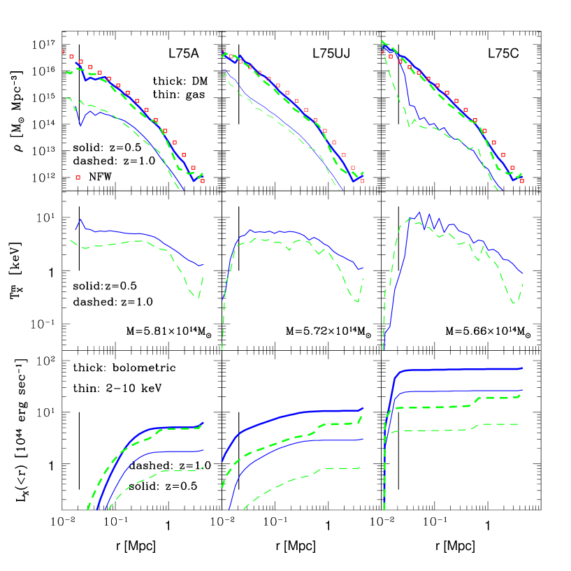
Figure 2: Same as Figure 1 but for models L75A, L75UJ, and L75C at $z=0.5$ (solid lines) and $z=1.0$ (dashed lines). The virial mass of each cluster at $z=0.5$ is quoted in the middle panels.

In Figure 1, we show the spherically averaged profiles of dark matter and gas densities, ICM temperature, and cumulative X-ray luminosity for the most massive cluster in models L150A, L150UJ and L150C. Those for models L75A, L75UJ and L75C are also depicted in Figure 2. The centers of clusters are defined as the peaks of gas density. The profiles of dark matter are fairly well-approximated by the model proposed by (Navarro, Frenk, & White, 1997). Due to an artificial cooling catastrophe, the pure-cooling model (L150C and L75C) produces unacceptably high X-ray luminosity, consistent with Suginohara & Ostriker (1998). This artificial feature can be largely removed by decoupling the cold gas from hot component, and models L150UJ and L75UJ yield a fairly reasonable range of X-ray luminosities. Nevertheless we do not claim that the luminosities in L150UJ and L75UJ are reliable; the current modified scheme is to be interpreted as a tentative and phenomenological remedy at best and should be replaced by more realistic scheme for galaxy formation. Lewis et al. (1999) have obtained a very similar result based on a more sophisticated treatment of galaxy formation in their simulation. They show that when both cooling and star formation are included in the simulation, cluster luminosities increase only moderately (a factor 3) compared to the non-radiative case; this amount of increase is significantly less than that in the pure-cooling case. In addition, we find that the values of the luminosities are still significantly affected by the numerical resolution (§3.3).

In Figures 3 and 4, we show the spherically averaged profiles of local dynamical timescale $t_{\rm dyn}$, 2-body heating timescale $t_{\rm 2body}$ (Steinmetz & White, 1997) and cooling timescale $t_{\rm cool}$ for representative clusters with 3 different mass scale for models L150UJ and L75UJ, respectively. Each timescale is defined as

$$t_{\rm dyn} = \frac{1}{\sqrt{G\rho_{\rm\scriptscriptstyle{tot}}}},$$ (4)

$$t_{\rm 2body} = \sqrt{\frac{27}{128\pi}}\frac{\sigma^{3}_{\rm 1D}}{G^{2}M_{{\rm\scriptscriptstyle{DM}}}\rho_{{\rm\scriptscriptstyle{DM}}}\ln\Lambda},$$ (5)

$$t_{\rm cool} = \frac{3n_{\rm\scriptscriptstyle{gas}}k_{\rm B}T}{2\Lambda_{\rm cool}(n,T)},$$ (6)

where $G$ is the gravitational constant, $\rho_{\rm\scriptscriptstyle{tot}}$ the total mass density , $\sigma_{\rm 1D}$ the 1-dimensional velocity dispersion of dark matter particles, $\ln\Lambda$ the Coulomb logarithm, $M_{{\rm\scriptscriptstyle{DM}}}$ the mass of a dark matter particle, $\rho_{{\rm\scriptscriptstyle{DM}}}$ the mass density of dark matter, $n_{\rm\scriptscriptstyle{gas}}$ the number density of gas, $k_{\rm B}$ the Boltzmann constant and $\Lambda_{\rm cool}(n,T)$ the cooling function. The expression for $t_{\rm 2body}$ is given in Steinmetz & White (1997) and we set the value of the Coulomb logarithm to $\ln\Lambda=5$ as a nominal value.

For the clusters with $M\gtrsim 2\times 10^{14}\,M_{\odot}$ in the models with $L_{\rm box}=150h^{-1}\mbox{Mpc}$ , $t_{\rm cool}$ is shorter than $t_{\rm 2body}$, and hence the artificial 2-body heating is not effective for these clusters. On the other hand, clusters with $M\lesssim 10^{14}M_{\odot}$ have the cooling timescale comparable with the 2-body heating timescale. Thus, the relatively poor clusters with $M\lesssim 10^{14}M_{\odot}$ in $L_{\rm box}=150h^{-1}\mbox{Mpc}$ models may suffer from the artificial 2-body heating. Since it is difficult to predict the possible systematic effect based on the timescale argument alone, it is most straightforward to quantify the effect by a careful comparison with the results in $L_{\rm box}=75h^{-1}\mbox{Mpc}$ runs which are almost free from the artificial 2-body heating. In the following analysis, we use clusters with $M>10^{14}M_{\odot}$ and $M>10^{13}M_{\odot}$ for L150 and L75 models, respectively. Table 2 indicates the number of those clusters which satisfy the above criteria for each model at different redshifts.

It should also be noted that one should not worry the numerical 2-body heating at the central regions of clusters where $t_{\rm dyn}\gg t_{\rm cool}$ even if $t_{\rm cool}\gtrsim t_{\rm 2body}$. As noted in Steinmetz & White (1997), those regions will experience a catastrophic cooling; in fact, they are exactly the place where we attempt to suppress the overcooling by decoupling the cold gas particles.

3.2 Temperature – mass relation

A conventional analytical modeling of clusters of galaxies assumes that the ICM is isothermal and in hydrostatic equilibrium within the dark matter potential. Then the ICM temperature is predicted to be

$$k_{\rm B}T_{X}=\gamma\frac{\mu m_{\rm p}GM}{3r_{\rm vir}}$$ (7)

$$\sim 5.2\gamma\left(\frac{\Omega_{0}\Delta_{\rm c}}{18\pi^{2}}\right)^{1/3}\left(\frac{M}{10^{15}h^{-1}M_{\odot}}\right)^{2/3}(1+z_{\rm f})\,\mbox{keV}$$ (8)

in terms of the cluster mass $M$, where $\Delta_{\rm c}$ is the mean density of a virialized object at a formation redshift $z_{\rm f}$, and $\gamma$ is a fudge factor of an order unity; if the cluster is isothermal and its one-dimensional velocity dispersions is equal to $\sqrt{GM/3r_{\rm vir}}$, then $\gamma$ is the inverse of the spectroscopic $\beta$-parameter and approximately given by $1.2$ (Kitayama & Suto, 1997).

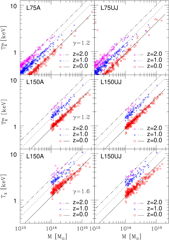
Figure 5: Temperature–mass relations for non-radiative and multiphase models at $z=0.0$, $1.0$ and $2.0$. The lowest panels show the emission-weighted temperature while others the mass-weighted temperature. Lines indicate the theoretical model (eq.[8]) with $\gamma=1.6$ for emission-weighted temperature, and $\gamma=1.2$ for mass-weighted one.

Since the above $T_{X}$–$M$ relation is the most important ingredient in translating the Press – Schechter mass function into the XTF, the reliability of the conventional cluster abundance crucially depends on the applicability of this relation. Figure 5 plots the $T_{X}$–$M$ relations for non-radiative and multiphase models at $z=2$, 1 and 0. In order to avoid the possible artificial two-body heating effect, we show the results for clusters of $M>10^{13}\,M_{\odot}$ and $M>10^{14}\,M_{\odot}$ in L75 and L150 models, respectively.

This figure implies three major conclusions; first, comparison of the upper and middle panels indicates that the current numerical resolution is sufficiently good and the $T_{X}$–$M$ relation seems to be converged. Second, the mass weighted temperature $T_{X}^{\rm m}$ is well fitted to equation (8) with $\gamma=1.2$, while the emission weighted temperature $T_{X}$ is systematically higher for the same $M$. Finally, the simulated $T_{X}$–$M$ relation is almost unaffected by the phenomenological (in the current simulation) treatment of the thermal evolution of the ICM gas, and the results of L150A and L150UJ are almost identical. We also verify that the results of L150CJ are almost identical to those of L150UJ implying that the presence of a UV background does not affect our conclusions. This is the first successful check of the relation, made possible by the sufficiently large volume and good resolution of our simulations.

3.3 Luminosity – temperature relation

In contrast to the $T_{X}$–$M$ relation, the luminosity – temperature relation of X-ray clusters is not easy to predict. This is because the X-ray luminosity is proportional to the square of the gas density, and thus sensitive to the thermal evolution of the ICM. A simple self-similar model, which predicts $L_{X}\propto T_{X}^{2}(1+z_{\rm f})^{3/2}$ (Kaiser, 1986), is shown to be completely inconsistent with the observed relation of $L_{X}\propto T_{X}^{\alpha}(1+z)^{\zeta}$ where $2.6\lesssim\alpha\lesssim 3.0$ and $\zeta\simeq 0$ (Edge & Stewart, 1991; David et al., 1993; Markevitch, 1998).

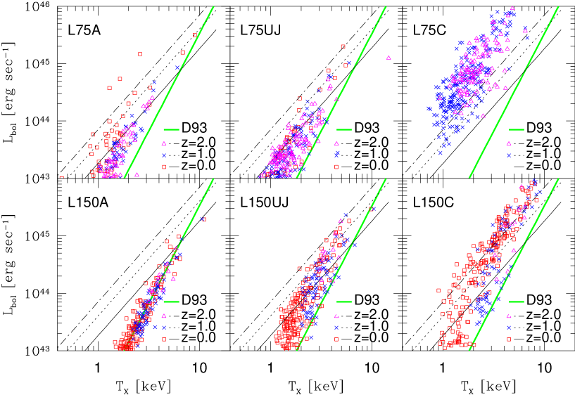
Figure 6: Luminosity–temperature relations for non-radiative and multiphase models at $z=0.0$, 1.0 and 2.0. Thin lines indicate the relations predicted from the self-similar evolution. Bold lines indicate the empirical relation from observations (David et al. 1993).

The $L_{X}$ – $T_{X}$ relation of our simulated clusters (Fig. 6) also exhibits the difficulty to obtain a reliable estimate of the luminosities. While it is reasonable that the results are sensitive to the ICM thermal evolution, they are also affected by the numerical resolution. The cluster luminosities in $L_{\rm box}=150h^{-1}$Mpc models are systematically underestimated relative to those in $75h^{-1}$Mpc models. Since we employ the equal-mass particle in the simulations, the resolution problem would be more serious for smaller clusters. Actually this explains why L150A model produces $L_{X}\propto T_{X}^{3}$ accidentally although this non-radiative model should result in $L_{X}\propto T_{X}^{2}$. Thus we conclude that the reliable estimate of the X-ray luminosities requires much higher resolution, especially for less luminous clusters, than ours in addition to the more physical implementation of the galaxy formation process. Therefore, we disagree with Pearce et al. (1999b) who concluded that the effect of cooling suppresses the X-ray luminosities; while our results do not reach convergence either, we find the opposite trend, i.e., the luminosities increase with the cooling (Figs. 1 and 6). After all, since their resolution is similar to ours, their results cannot escape from the resolution problem, and it is premature to draw any conclusion on the luminosities from cosmological SPH simulations.

3.4 X-ray Temperature Function

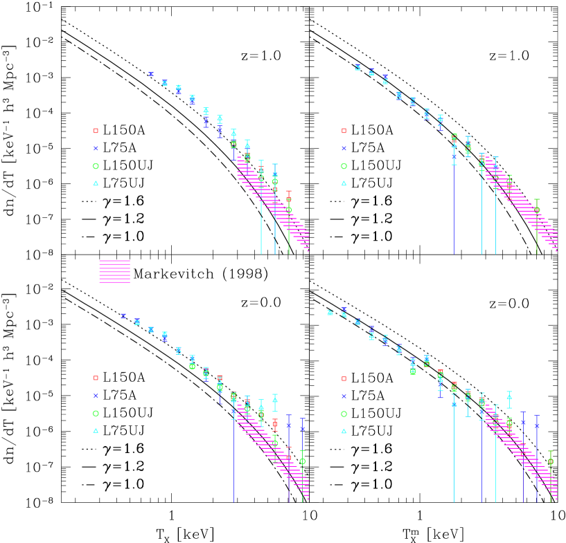
Figure 7: X-ray temperature functions at $z=0.0$ (lower panels) and $z=1.0$ (upper panels) for each model. The left panels uses emission weighted temperature, whereas the right ones mass weighted temperature. Lines are theoretical predictions using Press–Schechter mass function and $T$–$M$ relation (eq.[8]) with $\gamma=1.0$, 1.2 and 1.6. Shaded regions indicate the observed XTF of local ($z<0.1$) clusters by Markevitch (1998).

Finally we show the XTFs in non-radiative and multiphase models at redshift $z=0.0$ and $1.0$ (Fig. 7) as a function of the emission and mass weighted temperatures. These should be compared with the analytical prediction on the basis of the Press–Schechter mass function (Press & Schechter, 1974) and the $T_{X}$–$M$ relation mentioned above. Since we have already showed that the $T_{X}$–$M$ relation agrees well with the analytical expectation, our simulated clusters in cosmological volumes can examine the statistical reliability of the analytical prediction of XTF for the first time. Figure 7 implies that the analytical and numerical results agree well with each other almost independently of the ICM thermal evolution model; if we adopt $\gamma\simeq 1.6$ and $1.2$ for XTFs in terms of emission- and mass-weighted temperatures, respectively. It should be also noted that since the XTFs from different numerical resolutions are nearly the same within the statistical errors, we can state that the XTFs from our simulations do not suffer from any serious numerical artifacts. These results justify the use of a simple analytical model for the cluster abundance extensively applied before (White, Efstathiou & Frenk, 1993; Viana & Liddle, 1996; Eke, Cole & Frenk, 1996; Kitayama & Suto, 1997; Kitayama, Sasaki & Suto, 1998). The observed XTF of local ($z<0.1$) clusters by Markevitch (1998) is also shown in Figure 7 and lower by factor of 2–3 than the simulated ones at $T_{X}\simeq 3\mbox{--}9$ [keV].

4 Conclusions

On the basis of a series of the large cosmological SPH simulations, we have specifically addressed the reliability of the analytical predictions on the statistical properties of X-ray clusters. In order to distinguish numerical artifacts from real physics, we performed simulations with two different numerical resolutions. Our main findings are summarized as follows:

(i) The inclusion of radiative cooling in the high-resolution simulations substantially change the luminosity of simulated clusters. Without implementing the galaxy formation scheme, this leads to an artificial overcooling catastrophe as demonstrated by Suginohara & Ostriker (1998). With a phenomenological prescription of cold gas decoupling like Pearce et al. (1999a), however, the overcooling is largely suppressed. Nevertheless the predicted X-ray luminosities of clusters are not reliable even by one order of magnitude.

(ii) In contrast to the huge uncertainties on the X-ray luminosities, the temperature of simulated clusters is fairly robust both to the ICM thermal evolution and to the numerical resolution, and in fact are in good agreement with the analytic predictions commonly adopted. We also showed that the emission-weighted temperature is 1.3 times higher than the mass-weighted one.

(iii) The analytical predictions for the X-ray temperature function translated from the Press – Schechter mass function are fairly accurate and reproduce the simulation results provided that the fudge factor $\gamma=1.2(1.6)$ is adopted in the mass-weighted (emission-weighted) temperature – mass relation (8). The XTFs simulated in the cosmology adopted in this paper are slightly higher than the observed one of local clusters by Markevitch (1998).

Our simulations have made statistically unbiased synthetic catalogues of clusters of galaxies in virtue of their large simulation volume and sufficient numerical resolution. Thus, they can be the theoretical references which should be compared with the results from future cluster observations with X-ray satellites including XMM and Astro-E, and can contribute to probing cosmological parameters from observed cluster abundances in due course. Additional radiative processes such as heat conduction of ICM and energy feedback from supernovae explosions, which may considerably affect the physical properties of ICM, must be considered as future works in order to solve the discrepancy of $L$–$T$ relation. In addition, since we consider only one fairly specific cosmological model, it is necessary to perform simulations under other cosmological models.

Table 1: Summary of the simulation models

model	$L_{\rm box}$[Mpc]	cooling	$J_{21}^{0}$	$m_{\rm gas}[M_{\odot}]$	$m_{\rm dark}[M_{\odot}]$	cold gas decoupling
L150A	$150h^{-1}$	off	0.0	$2.0\times 10^{10}$	$1.7\times 10^{11}$	No
L150C	$150h^{-1}$	on	0.0	$2.0\times 10^{10}$	$1.7\times 10^{11}$	No
L150UJ	$150h^{-1}$	on	1.0	$2.0\times 10^{10}$	$1.7\times 10^{11}$	Yes
L150CJ	$150h^{-1}$	on	0.0	$2.0\times 10^{10}$	$1.7\times 10^{11}$	Yes
L75A	$75h^{-1}$	off	0.0	$2.4\times 10^{9}$	$2.2\times 10^{10}$	No
L75C	$75h^{-1}$	on	0.0	$2.4\times 10^{9}$	$2.2\times 10^{10}$	No
L75UJ	$75h^{-1}$	on	1.0	$2.4\times 10^{9}$	$2.2\times 10^{10}$	Yes

Table 2: Number of simulated clusters that we used in the analysis

model	$z=2.0$	$z=1.0$	$z=0.0$
L150A	12	72	224
L150UJ	11	76	220
L150C	12	75	222
L75A	123	263	295
L75UJ	117	241	272
L75C	120	245	—

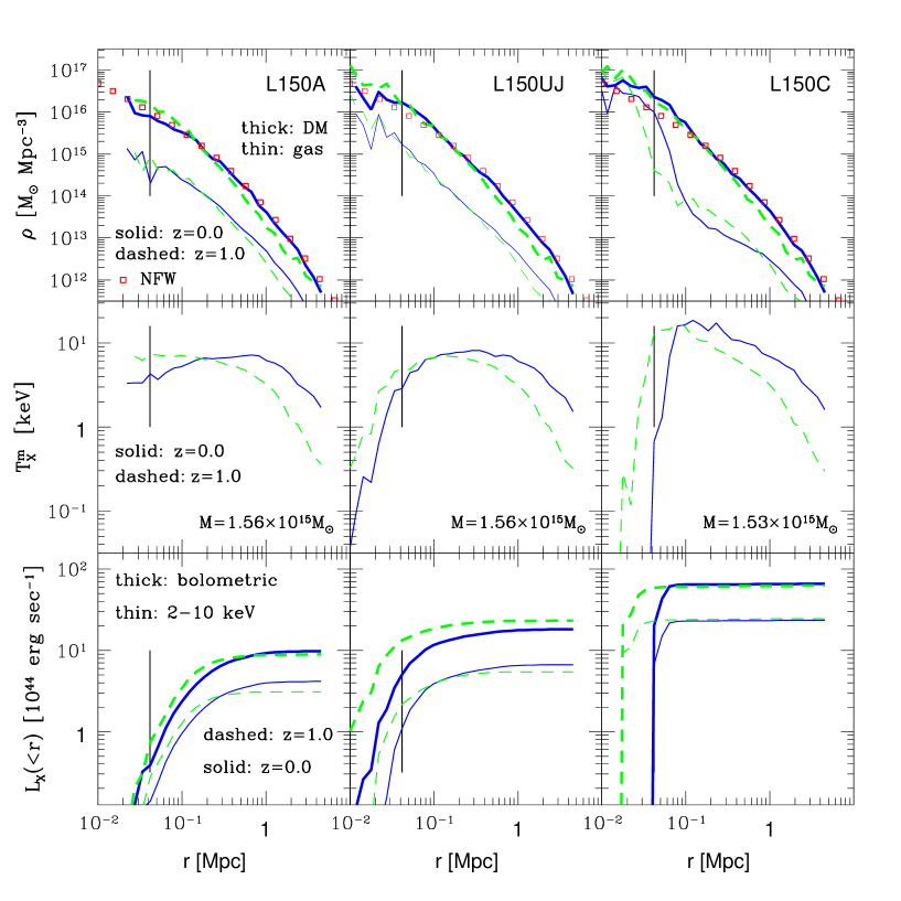
Figure 1: Spherically averaged profiles of dark matter and gas densities, ICM temperature and the integrated X-ray luminosity from the center, for a cluster at $z=0.0$ (solid lines) and $z=1.0$ (dashed lines) in models L150A, L150UJ and L150C. Vertical lines indicate our lower limit on the SPH smoothing length, $h_{\rm min}$. The viral mass of each cluster at $z=0.0$ is quoted in the middle panels. For reference, the universal density profile at $z=0$ (Navarro, Frenk, & White, 1997) corresponding to the virial mass of the cluster is plotted in open squares (top panels).

Figure 3: Radial profiles of the local dynamical timescale, $t_{\rm dyn}$, the artificial two-body heating timescale $t_{\rm 2body}$ and the cooling timescale $t_{\rm cool}$ for three different clusters at $z=0.0$ (lower panels) and $z=1.0$ (upper panels) in model L150UJ. Their virial mass and temperature are indicated in each panel.

Figure 4: Same as Figure 3 but for model L75UJ.

References

- Bertschinger (1995) Bertschinger, E. 1995, astro-ph/9506070
- Bryan & Norman (1998) Bryan, G.L. & Norman, M.L. 1998, ApJ, 495, 80
- Bunn & White (1997) Bunn, E.F. &White, M. 1997, ApJ, 480, 6
- Cen & Ostriker (1992) Cen, R. & Ostriker, J.P. 1992, ApJ, 393, 417
- Cen & Ostriker (1994) Cen, R. & Ostriker, J.P. 1994, ApJ, 429, 4
- Cen & Ostriker (1999) Cen, R. & Ostriker, J.P. 1999, ApJ, in press (astro-ph/9903207)
- Copi et al. (1995) Copi, C.J., Schramm, D.N. & Turner, M.S. 1995, ApJ, 455, 95
- David et al. (1993) David, L.P., Slyz, A., Jones, C., Forman, W. & Vrtilek, S.D. 1993, ApJ, 412, 479
- Edge & Stewart (1991) Edge, A.C. & Stewart, G.C. 1991, MNRAS, 252, 428
- Eke, Cole & Frenk (1996) Eke, V.R., Cole, S. & Frenk,C.S. 1996, MNRAS, 282, 263
- Eke, Navarro & Frenk (1998) Eke, V.R., Navarro,J.F. & Frenk,C.S. 1998, ApJ, 503, 569
- Evrard (1990) Evrard, A.E. 1990, ApJ, 363, 349
- Frenk et al. (1999) Frenk, C.S. et al. 1999, ApJ, 525, 554
- Henry & Arnaud (1991) Henry, J.P. & Arnaud, K.A. 1991, ApJ, 372, 410
- Hockney & Eastwood (1981) Hockney, R.W. & Eastwood, J.W. 1981, Computer Simulation Using Particles (New York: McGraw Hill)
- Jing & Fang (1994) Jing, Y.P. & Fang, L.Z. 1994, ApJ, 432, 438
- Jing & Suto (1998) Jing, Y.P. & Suto, Y. 1998, ApJL, 494, L5
- Kaiser (1986) Kaiser, N. 1986, MNRAS, 222, 323
- Kang et al. (1994) Kang, H., Cen, R., Ostriker, J.P. & Ryu, D. 1994, ApJ, 428, 1
- Katz, Weinberg & Hernquist (1996) Katz, N., Weinberg, D.H. & Hernquist, L. 1996,ApJS, 105, 19
- Kitayama, Sasaki & Suto (1998) Kitayama, T., Sasaki, S. & Suto, Y. 1998, PASJ, 50, 1
- Kitayama & Suto (1996) Kitayama, T. & Suto, Y. 1996, ApJ, 469, 480
- Kitayama & Suto (1997) Kitayama, T. & Suto, Y. 1997, ApJ, 490, 557
- Lacey & Cole (1994) Lacey, C. & Cole, S. 1994, MNRAS, 271, 676
- Lewis et al. (1999) Lewis, G.F., Babul, A., Katz, N., Quinn, T., Hernquist, L. & Weinberg, D.H. 1999, astro-ph/9907097
- Markevitch (1998) Markevitch, M. 1998, ApJ, 504, 27
- Navarro, Frenk, & White (1997) Navarro, J.F., Frenk, C.S., & White, S.D.M. 1997, ApJ, 490, 493
- Pearce et al. (1999a) Pearce, F.R., Jenkins, A., Frenk, C.S., Colberg, J.M., White, S.D.M., Thomas, P.A., Couchman, H.M.P., Peacock, J.A. & Efstathiou, G. 1999, ApJL, 521, L99
- Pearce et al. (1999b) Pearce, F.R., Couchman, H.M.P., Thomas, P.A. & Edge, A.C. 1999, astro-ph/9908062
- Press & Schechter (1974) Press, W.H. & Schecter, P. 1974, ApJ, 187,425
- Rybicki & Lightman (1979) Rybicki, G.B. & Lightman, A.P. 1979, Radiative Processes in Astrophysics (New York;Wiley)
- Steinmetz & White (1997) Steinmetz, M. & White, S.D.M. 1997, MNRAS, 288, 545
- Suginohara & Ostriker (1998) Suginohara, T. & Ostriker, J.P. 1998, 507, 16
- Suto (1993) Suto, Y. 1993, Prog.Theor.Phys., 90, 1173
- Suto et al. (1992) Suto, Y., Cen, R. & Ostriker, J.P. 1992, ApJ, 395, 1
- Thacker et al. (1998) Thacker, R.J., Tittley,E.R., Pearce, F.R., Couchman, H.M.P. & Thomas, P.A. 1998, astro-ph/9809221
- Ueda, Itoh & Suto (1993) Ueda, H., Itoh, M. & Suto, Y. 1993, ApJ, 408, 3
- Vedel et al. (1994) Vedel, H., Hellsten, U. & Sommer-Larsen, J. 1994, MNRAS, 271, 743
- Viana & Liddle (1996) Viana, P.T.P. & Liddle, A.R. 1996, MNRAS, 281, 323
- White, Efstathiou & Frenk (1993) White, S.D.M., Efstathiou, G. & Frenk, C.S. 1993, MNRAS, 262, 1023
- Yoshikawa, Itoh & Suto (1998) Yoshikawa, K., Itoh, M. & Suto, Y. 1998, PASJ, 50, 203