The Rise Times of High and Low Redshift Type Ia Supernovae are Consistent

Abstract

We present a self-consistent comparison of the rise times for low– and high–redshift Type Ia supernovae. Following previous studies, the early light curve is modeled using a $t^{2}$ law, which is then mated with a modified Leibundgut template light curve. The best-fit $t^{2}$ law is determined for ensemble samples of low– and high–redshift supernovae by fitting simultaneously for all light-curve parameters for all supernovae in each sample. Our method fully accounts for the non-negligible covariance amongst the light-curve fitting parameters, which previous analyses have neglected. Contrary to Riess et al. (1999a), we find fair to good agreement between the rise times of the low– and high–redshift Type Ia supernovae. The uncertainty in the rise time of the high-redshift Type Ia supernovae is presently quite large (roughly $\pm 1.2$ days statistical), making any search for evidence of evolution based on a comparison of rise times premature. Furthermore, systematic effects on rise-time determinations from the high-redshift observations, due to the form of the late-time light curve and the manner in which the light curves of these supernovae were sampled, can bias the high-redshift rise-time determinations by up to ${}^{+3.6}_{-1.9}$ days under extreme situations. The peak brightnesses — used for cosmology — do not suffer any significant bias, nor any significant increase in uncertainty.

1 Introduction

Two independent research groups have presented compelling evidence for an accelerating universe from the observation of high-redshift Type Ia supernovae (SNe Ia) (Perlmutter et al., 1999; Riess et al., 1998). These findings have such important ramifications for cosmology that every effort must be made to thoroughly test the calibrated standard candles on which they are based. Indeed, these groups, and others, are pursuing additional observations at both high- and low-redshift to confirm these results. There are programs in place aimed at reducing the statistical errors, testing systematic errors, limiting the amount of absorption due to grey dust (Aguirre, 1999), and searching for signs of evolution as a function of redshift in SNe Ia.

Recently Riess et al. (1999a) attempted to examine the question of whether the rise times of SN Ia evolve. They used new low-redshift SNe Ia light-curve photometry from Riess et al. (1999b) to compare the mean rise time of these SNe Ia to a preliminary rise time for high-redshift SNe Ia given in a conference abstract by Groom (1998) and based on a composite light curve derived from Supernova Cosmology Project (SCP) observations. Riess et al. noted a 5.8-$\sigma$ difference between the rise times from the low-redshift data and from the Groom (1998) preliminary analysis of high-redshift data, with the high-redshift supernovae having shorter rise times by 2.4 days. Based on this result, they suggested the possibility that SNe Ia undergo sufficient evolution to account for what has been interpreted as evidence for an accelerating universe.

In what follows, we address major shortcomings of these earlier analyses which fundamentally alter the conclusion of Riess et al. (1999a). Specifically, the analysis method used in Groom (1998) to produce a high-redshift rise-time estimate is very different than that used to produce the low-redshift rise-time estimate of Riess et al. (1999a). Furthermore, both analyses neglected correlated uncertainties in the light-curve fit parameters, and amongst the light-curve data points, so neither of these analyses is complete. We also examine, in $\S 3$, the role of light-curve sampling differences between the low-redshift and high-redshift SN Ia observations and how they can conspire with systematic deviations from the fitted reference template — seen for normal SNe Ia — to shift the inferred rise time. In $\S 4$ we briefly discuss the (small) impact on the cosmological application of SNe Ia resulting from light-curve variations. We conclude in $\S 5$ with a summary of our results and a discussion intended to help guide future work on the question of whether SNe Ia evolve.

2 Statistical Analysis of SNe Ia Rise Times

2.1 Description of the Problem

Figure 1 illustrates the full SN Ia template, $\psi(t)$, normally used by the SCP, which is a modified version of the Leibundgut template (Leibundgut, 1988; Perlmutter et al., 1997). The light-curve fitting parameters are the peak flux, $f_{max}$, time of maximum, $t_{max}$, and light curve stretch, $s$. (Note that all time dependent quantities refer to the rest frame of the supernova.) Goldhaber (1998) has demonstrated the remarkable fact that the stretch method applies to the rising portion of SN Ia light curves as well as it applies to the declining portion (up to +25 days after maximum) to better than 2% of the peak flux. This has been confirmed for nearby SNe Ia by Riess et al. (1999b). One can represent the flux light curve, $f(t)$, as follows:

$$f(t)=f_{max}\psi((t-t_{max})/s)$$

This approach works well in the $U-$, $B-$ and $V-$bands over the range $-20\ {\rm days}<t-t_{max}<+25\ {\rm days}$ (see both Perlmutter et al. (1999) and Perlmutter et al. (1997) for a full explanation of the use of this approach).

Figure 1: The modified Leibundgut template used by the SCP (Perlmutter et al., 1999, 1997), with the standard light-curve fitting parameters, $f_{max}$, $t_{max}$, and $s$ labeled. Also shown are two examples from the grid of $t^{2}$ laws mated to the modified Leibundgut template used to perform the statistical fits discussed in the text. The $t^{2}$ law is parameterized using an explosion day, $t_{exp}$, and a date, $t_{join}$, at which the $t^{2}$ law mates with the modified Leibundgut template.

A meaningful comparison of rise times for low– and high–redshift supernovae requires that both datasets be fit with the same template, and that the fits be performed in a manner which fully accounts for the covariance between the light-curve fitting parameters and the calculated rise time. For the high-redshift data, accounting for covariance in the light-curve fitting parameters is especially important since the uncertainties on individual data points are relatively large. Such uncertainties allow the fitted date of maximum light, $t_{max}$, the peak brightness, $f_{max}$, and the light-curve width, $s$, to be changed in compensating ways to yield similarly good fits. Thus, these parameters are correlated, and since determination of the rise time or explosion date, $t_{exp}$, involves both $s$ and $t_{max}$, it is incorrect to fit for these parameters while holding $s$ and $t_{max}$ fixed.

Take for example the case where the fitted value of $t_{max}$, $t_{max}^{\prime}$, is too early by 1 day. The fitted value of $s$, $s^{\prime}$, will suffer a compensating increase by roughly $1/15$ in an effort to fit the data on the fast-declining, well-sampled portion of the light curve at $+10<t-t_{max}<+20\ {\rm days}$. The effective stretch-corrected epoch, $t_{s}=(t-t_{max})/s$, of a point nominally at $t-t_{max}=-20$ days and for $s=1$ would be incorrect by:

$$\Delta t_{s}=(t-t_{max})/s-(t-t_{max}^{\prime})/s^{\prime}$$

$$=\frac{-20}{1.00}-\frac{-19}{1.07}=-2.2\ {\rm days}.$$

Likewise, if $t_{max}^{\prime}$ were 1 day after $t_{max}$, $s^{\prime}$ would be smaller than the true $s$, changing $\Delta t_{s}$ by roughly $+2.5$ days. This is the principal mechanism by which uncertainties in the light-curve fit parameters propagate into increased uncertainty in SN Ia rise times. (Our Monte Carlo simulations in §3 bear this out.) If the uncertainties in $t_{max}$ and $s$ had simply been propagated as if they were independent, the assigned uncertainty would be 1.7 days, and the correlated nature of the uncertainties would be lost. It is true that a point at $t-t_{max}=-20$ days may also play some role in constraining $s$. However, for the datasets considered here the observations on the rising portion of the light curves are generally much less certain than those on the declining portion.

The analyses presented in Groom (1998) and Goldhaber (1998) were designed to test the efficacy of the stretch technique when applied to the rising portion of the light curves of high-redshift supernovae, and to attempt to improve that portion of the SCP light curve template. The high-redshift data from the SCP were aligned to stretch-corrected epochs, $t_{s}$, using $t_{max}$ and $s$ for each supernova determined from individual light-curve fits without exclusion of data from any light-curve epoch. Then a $t^{2}$ rise-time model was fit to the ensemble pre-max data, with the final result quoted for $t^{2}$ fits covering rest-frame epochs $-21$ to $-10$ days with respect to $t_{max}$. None of the uncertainty due to the light-curve fitting parameters was propagated into the final quoted rise-time uncertainty (Goldhaber, 1999, private communication). The resulting $t^{2}$ fit was then used to develop a revised template, and the individual SNe Ia light curves were then re-fit to this revised template.

Riess et al. (1999a) analyzed the low-redshift data very differently: they aligned their low-redshift data using $t_{max}$ and $s$ for each supernova as in the preliminary high-redshift analysis, but they used only data from $-10$ to $+35$ days to fit the light curves. After aligning the light curves, a $t^{2}$ rise-time model was fit to the ensemble pre-max data, with the final result quoted for $t^{2}$ fits covering rest-frame epochs $-23$ to $-10$ days. Following Riess et al. (1999b), the uncertainty in $t_{max}$ and $s$ was accounted for in Riess et al. (1999a) by increasing the uncertainties on the stretch-corrected light-curve photometry points. The modest contribution due to correlated uncertainties was not included.

Both of these studies fixed $t_{max}$ and $s$ for the individual SNe Ia before fitting the $t^{2}$ model from which explosion dates were inferred. They propagated the uncertainties in the light-curve fits parameters in an incomplete and approximate way. Since this approach does not allow each individual supernova’s light-curve fit parameters, $f_{max}$, $t_{max}$, and $s$, to adjust to give the best fit as different rise times are tested, the uncertainties quoted in these studies are likely to be underestimates. In addition, since the two studies fit to different time intervals of data, a comparison of the central values may not be self-consistent.

2.2 Fitting Method

The most assumption-free means of accounting for how the uncertainties in the fits to individual SNe Ia light curves affect the value and uncertainty of the rise time is to explicitly test various rise times to see how well the SNe Ia are able to adjust to give fits of similar quality. This is more accurate than, and avoids difficulties associated with, attempting to propagate uncertainties based on the covariance matrix determined at the best-fit value when dealing with complex parameter probability spaces, such as those which occur for some SNe Ia light curves dealt with here. This approach requires that a family of templates with different rise times be defined and fit to the entire photometric dataset for each SN Ia.

Unfortunately, at present, very little light-curve data are available for determining a suitable early-epoch template for a SN Ia. Therefore we have constructed a grid of templates consisting of $t^{2}$ models starting with zero flux at an explosion epoch, $t_{exp}$, and joined to the modified Leibundgut template at epoch, $t_{join}$. A $t^{2}$ model can be justified under the conditions of uniform expansion and constant effective temperature from simple physics (see also Arnett (1982)). Two examples from this family of $t^{2}$-model, $t_{exp}$, $t_{join}$ templates are shown in Figure 1, with the epochs $t_{exp}$ and $t_{join}$ labeled. These can be compared to the modified Leibundgut template, which is known to be a reasonable approximation to the light curves of many SNe Ia (with the timescale stretched or contracted).

Note that the use of $t_{exp}$, $t_{join}$ to describe the early-epoch light curve is simply a reparameterization of the $\alpha,t_{exp}^{2}$ models (i.e., $f(t)=\alpha(t-t_{exp})^{2}$) used in previous studies, with the added constraint of continuity where the $\alpha,t_{exp}^{2}$ model ends and the modified Leibundgut template begins. Riess et al. (1999a) did not impose a continuity constraint since the fitting to the early stretch-corrected light curve with an $\alpha,t_{exp}^{2}$ model was performed after (some portion) of the original light curve was fit with another template. Groom (1998) and Goldhaber (1998) have an implicit continuity constraint in that they mated their best-fit $t_{exp}^{2}$ model to the remainder of their light curve when constructing each new template. In this paper the fit for the rise time and the overall light-curve parameters is performed simultaneously.

An added benefit of our parameterization is that $t_{exp}$, $t_{join}$ are more nearly orthogonal than $\alpha,t_{exp}^{2}$. This is because the already-established modified Leibundgut template provides a strong constraint on the amplitude of a $\alpha$, $t_{exp}^{2}$ model at the point it crosses the modified Leibundgut template. $\alpha$ simply adjusts itself to satisfy this constraint as $t_{exp}$ is changed. (This leads to the narrow, but strongly tilted, confidence regions in Figure 1 of Riess et al. (1999a)).

The fitting method we use integrates the probability [$P\propto exp(-\chi^{2}/2)$; see Eq. 28.22 in Ceolin et al. (1998) ] over the parameters $f_{max}$, $t_{max}$, and $s$ separately for each supernova, at each value of $t_{exp}$, $t_{join}$. The fits are performed in flux (rather than magnitudes); this allows the use of non-detections, these being the principal source of early-epoch data for the Perlmutter et al. (1999) high-redshift supernovae. Two alternative methods are used to perform the integrations over $f_{max}$, $t_{max}$, and $s$. In the first, the integral over $f_{max}$ is performed analytically and the subsequent integration over $t_{max}$, and $s$ uses the adaptive integration algorithm of Berntsen et al. (1991). The second method uses a grid of $\Delta f_{max}=0.01$, $\Delta t_{max}=0.1$ days and $\Delta s=0.01$ centered on the averages of the best fit values over $t_{exp}$ for the high-redshift SNe Ia. To account for the tightly constrained parameters of the low-redshift SNe Ia a hybrid technique is used in which the integral over $f_{max}$ is done analytically and a grid of $\Delta t_{max}=0.01$ days and $\Delta s=0.0005$ is used to integrate over $t_{max}$ and $s$. In each, the limits are chosen such that the probabilities are negligible at the boundaries. We find excellent agreement between each of these methods.

The end product is a map of probability over $t_{exp}$, $t_{join}$ for each supernova. These probability maps are then multiplied, then renormalized, for an ensemble of supernovae, e.g., the high-redshift supernovae from Perlmutter et al. (1999) or the low-redshift supernovae of Riess et al. (1999a), to determine the joint probability distribution function over $t_{exp}$, $t_{join}$, $P(t_{exp},t_{join})$; or after normalizing over $t_{exp}$ for each $t_{join}$, the conditional probability distribution function for $t_{exp}$ given $t_{join}$, $P(t_{exp}|t_{join})$.

2.3 Supernova Light-Curve Samples

What we will hereafter refer to as the “low-redshift SNe Ia” sample consists of SN 1990N, SN 1994D, SN 1996bo, SN 1996bv, SN 1996by, SN 1997bq, SN 1998aq, SN 1998bu, and SN 1998ef, for which early-epoch light-curve photometry transformed to $B$-band from unfiltered CCD images has been reported by Riess et al. (1999b). The early-epoch photometry was supplemented with data from Lira et al. (1998); Patat et al. (1996); Meikle et al. (1996); Riess et al. (1999c); Suntzeff et al. (1999); Jha et al. (1999); Riess et al. (1999b) to produce full $B$-band light curves extending over peak and beyond. Riess et al. (1999b) reports four early-epoch light-curve points (one an upper limit) for SN 1998dh, however we were unable to include this supernova since the subsequent light-curve photometry was unavailable.

What we will hereafter refer to as the “high-redshift SNe Ia” sample consists of the 30 SNe Ia from Perlmutter et al. (1999) having redshift $0.35<z<0.65$, with the exception of SN 1997aj. As defined, this sample satisfies the requirements that at least 60% of the light in the $R$-band comes from the rest-frame $B$-band and that at least 60% of the rest-frame $B$-band light is included in the $R$-band. Redshift limits satisfying these conditions were determined using the $B$-band and $R$-band filter responses given in Bessel (1990), along with spectra of normal SNe Ia as a function of light-curve epoch constructed by Nugent et al. (2000). These restrictions allow comparison with the low-redshift $B$-band photometry of Riess et al. (1999a) while minimizing the potential uncertainties inherent in making large cross-filter K-corrections. Even so, K-correction uncertainties will be present for those supernovae near these redshift limits, as well as at very early times where few spectra are available from which K-corrections can be calculated. Note that most of the other eleven supernovae from Perlmutter et al. (1999) have complete light curves only in rest-frame $V$-band or $U$-band, and therefore are unsuitable for determination of the $B$-band light-curve parameters. Also note that not all 30 high-redshift SNe Ia have equal value in determining the rise time. Only those that were fortuitously caught on the rise in the reference images of the search run can constrain this region of the light curve.

2.4 Results of the Statistical Analysis

Templates were generated for $-29.9<t_{exp}<-10.1$ days, in steps of 0.2 days, and for $-20<t_{join}<-4$ days, in 1 day steps. Fitted templates were required to have $t_{exp}$ earlier than $t_{join}$. Figure 2 presents the results of these fits; shown are the 1–, 2–, and 3–$\sigma$ confidence regions for the conditional probability, $P(t_{exp}|t_{join})$, for the high-redshift SNe Ia sample. Also shown are points which mark the most probable value of $t_{exp}$ at each $t_{join}$ for the low-redshift SNe Ia sample. Figure 3 distills the $t_{exp}$ differences taken from Figure 2 into equivalent Gaussian standard deviations for the difference in $t_{exp}$ between the high-redshift and low-redshift SNe Ia samples. These plots demonstrate that for $t_{join}<-10$, the high-redshift and low-redshift SNe Ia samples agree at the 1-$\sigma$ level or better. For $t_{join}$ less than $\sim-15$ days, the high-redshift SNe Ia sample is unable to place meaningful constraints on $t_{exp}$.

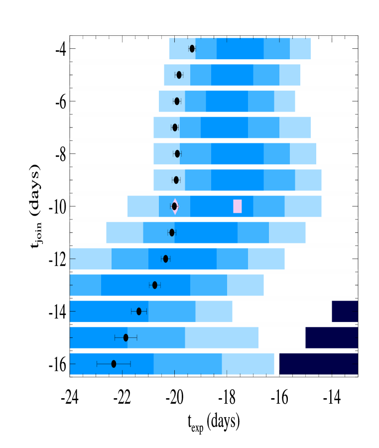
Figure 2: The 1–, 2–, and 3–$\sigma$ (68.3%, 95.4%, and 99.73%, in progressively lighter shades of blue) confidence regions for the conditional probability of $t_{exp}$ given $t_{join}$, $P(t_{exp}|t_{join})$, for the high-redshift SNe Ia sample. The small solid circles are our results for the maximum-likelihood $t_{exp}$ for a given $t_{join}$ for the low-redshift sample. The uncertainties in $t_{exp}$ for these points vary from 0.14 days at $t_{join}=-4$ to 0.64 days at $t_{join}=-16$. For most values of $t_{join}$, the values of $t_{exp}$ for the low-redshift and high-redshift samples are in fair to good agreement. The large solid diamond represents the best-fit $t_{exp}$ for the low-redshift supernovae found by Riess et al. (1999a), for $t_{join}=-10$ days. The large solid square is the best-fit $t_{exp}$ for the high-redshift supernovae from the preliminary work of Groom (1998) and Goldhaber (1998). The best-fit values found in this work for $t_{join}=-10$ days are in good agreement with these previous studies, especially given the larger uncertainties (mainly for the high-redshift SNe Ia sample) we find with our analysis. Note that the region $t_{exp}<t_{join}$ (shaded in black) is physically excluded by the requirement that a supernova light curve be a single-valued function of time.

Figure 3: The equivalent number of Gaussian standard deviations by which the best-fit $t_{exp}$ for the low-redshift SNe Ia sample differs from that for the high-redshift SNe Ia sample, for each value of $t_{join}$. This calculation accounts for the uncertainties in $t_{exp}$ from both datasets. The difference of 1.5$\sigma$ at $t_{join}=-10$ days is shown as a point of reference, as the studies of Riess et al. (1999a); Groom (1998); Goldhaber (1998) have fit $t^{2}$ laws up through -10 days (to data that was pre-aligned by light-curve epoch and stretch). Note that for any value of $t_{join}$ the differences are much less than the 5.8 standard deviations found by Riess et al. (1999a).

The rise-time value quoted in Riess et al. (1999a) of $t_{exp}=-19.98\pm 0.15$ — compared to $t_{exp}=-20.08\pm 0.19$ (statistical) obtained from our analysis — was determined for $t_{join}=-10$ days, and is plotted in Figure 2. Even at this reference epoch the disagreement between the high-redshift and low-redshift SNe Ia samples is only 1.5-$\sigma$, not the 5.8-$\sigma$ difference found by Riess et al. (1999a). The value of $t_{exp}=-17.6\pm 0.4$ days given in preliminary analysis of the high-redshift sample by Groom (1998) is also plotted in Figure 2. As Figure 2 shows, the main difference between our finding and that of Riess et al. (1999a) lies in different best-fit values and larger uncertainties for the high-redshift SNe Ia sample (differing by $-0.7$ days at $t_{join}=-10$ days). The uncertainties are larger, especially for the high-redshift SNe Ia sample, when uncertainties in the light-curve fit parameters, $f_{max}$, $t_{max}$, $s$ (and to a lesser extent amongst the photometry points) are fully taken into account. These larger uncertainties come about because the individual SNe Ia are given the proper freedom to adjust to templates away from the global best-fit template. Previous analyses have artificially suppressed this freedom, and have therefore underestimated the uncertainty on $t_{exp}$.

Given the large uncertainty in $t_{exp}$, potential perturbations from the systematic effects discussed in the next section, and the fair to good agreement in $t_{exp}$ between the low- and high-redshift SNe Ia for reasonable values of $t_{join}$, we consider a detailed analysis of the best $t_{join}$ unwarranted. Riess et al. (1999b) found that $\chi^{2}$ per degree of freedom deteriorated for their fits for $t_{join}>-8$ days, indicating that the simple $\alpha,t_{exp}^{2}$ model is not appropriate later than $-8$ days. A cursory examination of the joint probability, $P(t_{exp},t_{join})$, for our fits showed that the low-redshift SNe Ia sample prefers $t_{join}\sim-8$ days, where our analysis finds a modest disagreement between the low-redshift and high-redshift supernovae. However, the early low-redshift SNe Ia observations prefer a slightly different $t_{join}$; $P(t_{exp},t_{join})$ based on observations having $t-t_{max}<-6$ days gives a preferred $t_{join}\sim-12$ days, where high- and low-redshift rise times agree quite well. This mild tension within the low-redshift SNe Ia sample with regard to the preferred $t_{join}$ is somewhat less than the 2–$\sigma$ level. A similar, but weaker, situation is found for the high-redshift SNe Ia sample. This is not a complete surprise; as the following section demonstrates, there are systematic variations in the late-time light-curve behavior of SNe Ia (such as SN 1994D from the low-redshift SNe Ia sample) which can affect the preferred rise time. Furthermore, a best fit value of $t_{join}$ depends not only on the rise-time behavior, but also the accuracy of the modified Leibundgut template for $t_{join}\leq t-t_{max}\leq-4$ days (the latest $t_{join}$ tested). The relative probabilites at different values of $t_{join}$ include a contribution from the $\alpha,t_{exp}^{2}$ model for $t<t_{join}$ and from the Leibundgut template for $t>t_{join}$. Because the parameters ($t_{max}$ and $s$) for the modified Leibundgut template are driven largely by points with $t>-4$ days, any early-time mismatch between the modified Leibundgut template and the data will degrade the quality of the fit a different amount for different values of $t_{join}$. This effect should only be of importance for $t_{join}$ later than about $-10$ days, where the data are better and where the best-fit $\alpha,t_{exp}^{2}$ curves begin to depart from the (full) modified Leibundgut template. As things stand, the goodness of fit changes imperceptibly with $t_{join}$ for the high-redshift SNe Ia sample.

3 Systematic Effects

Given these findings from the statistical analysis it is clear that there is a reasonable consistency between the rise times of the high- and low-redshift SNe Ia. However, it is important to explore the possibility of systematic effects which have the potential to drive a fit to another location and/or increase the error bars further. One such effect arises from application of the stretch relationship when fitting an observed light curve with a given template.

As mentioned in $\S 2.1$, the stretch method works particularly well up to $t\sim+25$ days past maximum. After this point the light curve of a SN Ia leaves the photospheric phase and enters into the nebular phase. This is marked by a bend in the light curve between +25 and +35 days after maximum light where the rapid drop from peak brightness slows down into an exponential decline of the light curve. Since this exponential decline is governed mostly by the radioactive decay of ⁵⁶Co to ⁵⁶Fe one would not expect it to “stretch” like the earlier portion of the light curve. In fact, as seen in Leibundgut (1988), the slopes of the declines are very similar for a wide range of SNe Ia light-curve widths. This highlights one of the current limitations of the stretch method; the entire template, regardless of epoch, is stretched to fit the data. This is not just a problem for the stretch method, but for any of the current SN Ia template fitting methods, which all employ a one-to-one correlation between peak brightness and the shape of the light curve. This is a small effect compared to the peak flux and the typical photometric uncertainties in current low- and high-redshift data sets. However, it is important to consider its effect specifically on the measurement of the rise time.

The amplitude with respect to peak of the aforementioned exponential decline varies among SNe Ia. It turns out that the stretch method can compensate somewhat for these differing amplitudes, providing better fits in the $\chi^{2}$ sense, but at the expense of introducing a possible bias in $s$. Since the amplitude variations during the exponential decline become apparent at brightnesses similar to those on the rising portion of the light curve being studied here, and since the data are generally much better for the later portion of the light curve, the late-time light-curve behavior may bias determination of the rise time. The effect of this bias on the template fitting method was studied via a Monte Carlo simulation, as described below.

Figure 4a shows the modified Leibundgut template along with two other templates derived from the SNe Ia 1986G and 1994D (Phillips et al., 1987; Meikle et al., 1996; Patat et al., 1996). These supernovae were chosen because, among those SNe Ia with good late-time data, they produced the largest deviations from the modified Leibundgut template in the tail of the light curve. To produce these templates for the Monte Carlo simulations the data through day +15 for SNe 1986G and 1994D were adjusted to fit the modified, unity-stretch, Leibundgut template. The resulting adjustments were then applied to the data beyond day +15 using the stretch method. These adjusted late-time data were fit with a smooth curve through the bend in the light curve, followed by an exponential decline. These late-time curves were then mated to the modified, unity-stretch, Leibundgut template for $t<+15$ days to form complete templates.

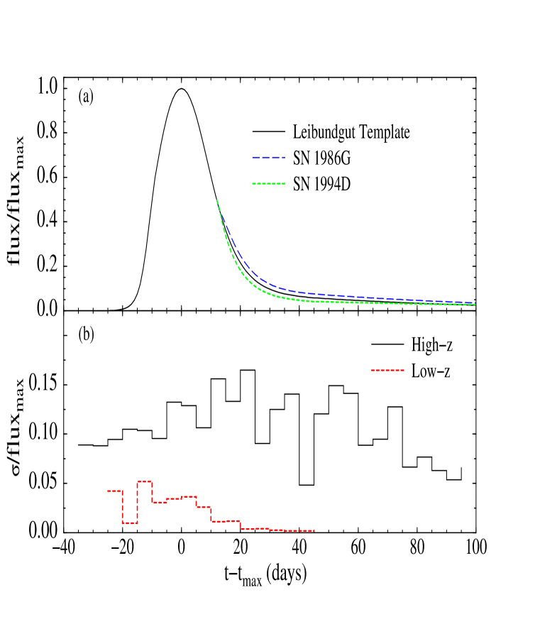
Figure 4: a) The different light-curves shapes used to study the systematic uncertainty due to temporal sampling and intrinsic light-curve deviations. The black curve corresponds to the standard modified Leibundgut template. The blue curve shows the late-time deviation exhibited by SN 1986G, while the green curve shows the late-time deviation for SN 1994D. b) The effective normalized ensemble uncertainty as a function of time for the high-redshift SNe Ia (black) and low-redshift SNe Ia (red) samples. If the observations from each of these samples had come from a single high-redshift or low-redshift supernova, this would reflect how well that light curve is determined. Although the uncertainty is not strongly dependent on light-curve phase for the high-redshift SNe Ia, the scale over which the data can be effectively averaged — set by the steepness of the light curve — leads to a poorer determination of the early, rising, portion of the light curve. Note also that the uncertainty is modulated slightly by lunar phase, since the SNe Ia are typically discovered shortly before maximum light and one week prior to new moon, and cannot be observed near full moon.

Figure 4b shows the normalized ensemble photometric error for both the high-redshift and low-redshift SN Ia samples in 7 day bins from $-35<t-t_{max}<+75$. This indicates how accurately a light curve would have been measured had all the observations come from just one supernova. Similarly, provided the stretch method works sufficiently well, and $f_{max}$, $t_{max}$, and $s$ are known, this would be the accuracy of a stretch-corrected composite light curve. Note that the high-redshift data are of consistent quality through $\sim 50$ days after maximum light, which enables the high-redshift SNe Ia sample data to constrain the fit to a template over a large range in time with nearly equal weight. However, this makes the high-redshift SNe Ia data susceptible to a systematic bias on the rise time due to possible deviations from the stretch fitting method for $t>40$ days for deviant light curves like those shown in Figure 4a.

The Monte Carlo simulation performed to test for such a bias created simulated light-curve photometry data for the three sets of supernovae based on the templates seen in Figure 4a. Each set was comprised of $\sim 100$ different realizations of each of the supernovae in the high-redshift SNe Ia sample based on their individual temporal sampling and associated photometry errors. All of the generated supernovae were created with the following input parameters: $s=1.0$, $t_{join}=-10.0$ days, $t_{exp}=-20.0$ days, $t_{max}=0.0$ and $f_{max}=1.0$. The resultant light curves produced in each set were fit with the modified Leibundgut template. $\chi^{2}$ surfaces of $t_{exp}$ and $t_{join}$ were created for each of the fits, and within a set these surfaces were added together to find the global minimum.

The results of these simulations are given in Table 1. It is apparent that given a set of SN Ia observations like those available from the high-redshift SNe Ia sample, a fit for $t_{exp}$ can be biased by 2—3 days in either direction if all the observed SNe Ia have deviant late-type light curves like SN 1986G or SN 1994D. To allow direct comparison with Figure 2, these same simulations were used to determine the best values of $t_{exp}$ for input templates with $t_{join}$ fixed at $-10.0$ days. For this case we found $t_{exp}=-19.8$, $-17.5$, and $-22.5$, when the data were simulated using the Leibundgut, SN 1986G, and SN 1994D templates, respectively. This shows that systematic errors in $t_{exp}$ are large even when $t_{join}$ is held fixed. While the SNe Ia template light curves used to simulate the high-redshift data can be thought of as extreme cases, at present the exact nature and frequency of such deviations at this light-curve phase is poorly quantified due to a lack of high-quality, well-sampled observations over peak and through day $\sim$ +60 for nearby supernovae. Therefore, this result should be taken as a rough upper limit on the systematic error on $t_{exp}$ due to temporal sampling and our current limited understanding of how the stretch relationship should be applied at late times.

Generating Template	$t_{exp_{in}}$	$t_{join_{in}}$	$t_{exp_{out}}$	$t_{join_{out}}$	$\Delta M_{B}^{corr}$
Leibundgut	$-20.00$	$-10.0$	$-19.76(62)$	$-8.01(42)$	$+0.006(011)$
SN 1986G	$-20.00$	$-10.0$	$-18.08(59)$	$-6.81(44)$	$+0.039(012)$
SN 1994D	$-20.00$	$-10.0$	$-23.62(19)$	$-8.84(20)$	$-0.020(009)$

Table 1: The resultant shift in $t_{join}$, $t_{exp}$ and $\Delta M_{B}^{corr}$ from our Monte Carlo simulations caused by generating SNe Ia from the above templates and fitting them with a Leibundgut template given the sampling and photometric errors in the SCP’s data set. RMS errors in the Monte Carlo simulations are in parens.

4 Cosmological Implications

Assuming all SNe Ia have rise times similar to that found by Riess et al. (1999b) from good early-time photometry, a light-curve template with $t_{exp}\sim-20$ days and $t_{join}\sim-10$ days might be a better template for use in fitting the light curves of SNe Ia at all redshifts. This raises the question of whether such a change from the modified Leibundgut template to a Riess–like template would alter the corrected peak magnitudes determined in Perlmutter et al. (1999). In comparing our fits to the high-redshift SNe Ia sample using these two alternative templates, we find no measurable change in the ensemble mean corrected peak magnitudes. We also find that no individual SN Ia changed by more than 0.02 magnitudes.

Another obvious question, addressed by the simulations of §3, is whether systematic variations in late-time light-curve behavior can affect the cosmological results of Perlmutter et al. (1999). In the last column of Table 1 we list $\Delta M_{B}^{corr}$, the change in the ensemble stretch-corrected peak magnitude for each dataset determined using the stretch-luminosity relation of Perlmutter et al. (1999). These changes ($-0.039<\Delta M_{B}^{corr}<0.020$) are small, and less than the systematic biases already considered in Perlmutter et al. (1999) (0.05 mag). Given the fact that these simulations represent the most extreme deviations encountered with our fitting method, we conclude that this bias has no effect on the determination of the cosmological parameters from SNe Ia.

5 Conclusions & Discussion

We find no compelling statistical evidence for a rise-time difference between nearby and distant SNe Ia, and therefore no evidence for evolution of SN Ia. We do find that for the high-redshift SNe Ia sample, temporal sampling coupled with real deviations of SNe Ia light curves at late-times could systematically bias the inferred rise time by 2—3 days. Even if present, these biases cannot dim the peak magnitudes by more than 0.02 magnitudes nor brighten them by more than 0.04 magnitudes even in the extreme cases that all the distant SNe Ia have late-time light curves like SN 1994D or SN 1986G, respectively. This leaves the cosmological results of Perlmutter et al. (1999) unchanged. Due to the large statistical uncertainties and possible systematic effects, we conclude that the extant photometry of high-redshift SNe Ia are in fact poorly suited for placing meaningful constraints on SN Ia evolution from their rise times.

If future studies using better early-epoch data (such as that expected from the SNAP satellite) were to find significant rise-time differences between nearby and distant SNe Ia, would this invalidate the use of SNe Ia as calibrated standard candles? This is a very complicated question. However, at least some models suggest that variations in the early rise-time behavior may be very sensitive to the spatial distribution of ⁵⁶Ni immediately after the explosion. Such differences would diminish as the SN Ia expands and the photosphere recedes, meaning that rise-time variations wouldn’t necessarily translate into differences in peak brightness (Pinto, 1999, private communication). Careful measurement of the rise time and the peak spectral energy distribution of individual SNe Ia will have to be carried out to address this question (see Nugent et al. (1995a, b) for a full description of the interplay between the rise time and the spectral energy distribution on the peak brightness of a SN Ia). It may even prove possible to use the rise time as an additional parameter to improve the standardization of SNe Ia.

We close with some general observations concerning the issue of SN Ia evolution. The peak brightnesses of SNe Ia are determined at some level by the underlying physical parameters of metallicity and progenitor mass, whose mean values can be expected to evolve with redshift. Nonetheless, there should exist nearby analogs for most distant SNe Ia since there is active star formation and a wide range of metallicities within nearby galaxies (Henry and Worthey, 1999; Kobulnicky and Zaritsky, 1999). The existing empirical relations between intrinsic luminosity and light-curve shape are able to homogenize almost all nearby SNe Ia. This implies that SNe Ia with some finite (but as yet poorly quantified) range of metallicities and progenitor masses can be used as calibrated standard candles. This forms the basis for using SNe Ia at high-redshift to probe the cosmology. If there is a dominant population of SNe Ia whose members are underluminous for their light curve shape at $z\sim 0.5$, as would be required to explain current observations in terms of evolution, there should be nearby examples of these SNe Ia. Such SNe Ia are not predominant among nearby SNe Ia, as almost all nearby SNe Ia obey a width-brightness relation. For such SNe Ia to predominate at $z\sim 0.5$ while being rare nearby requires a large reduction in their rate. Searches for SNe Ia conducted using exactly the same CCD-based wide-area blind-search methods used by the SCP find that the SNe Ia rate per comoving volume element does not change significantly between $z<0.1$ (Aldering, 2000), $z\sim 0.5$ (Pain et al., 1996, 2000, in preparation), and $z\sim 1.2$ (Aldering et al., 2000, in preparation). For the global rates to stay roughly constant while the rate of such hypothetical subluminous SNe Ia changes by an order of magnitude would be remarkable. For instance, a shift from Pop II progenitors at $z\sim 0.5$ to Pop I progenitors nearby would result in suppressed rates at $z\sim 0.5$. This is due to the fact that Pop II stars are a minor contributor to the luminosity density out to $z\sim 0.5$ (Shimasaku and Fukugita, 1998). Quantifying these arguments is beyond the scope of this paper, so we do not claim they as yet place a bound on SN Ia evolution. However, such arguments should be borne in mind when weighing the likelihood that the calibrated peak brightnesses of SNe Ia evolve. These arguments can also provide a partial basis for rigorous testing of the SN Ia evolution hypothesis.

References

- Aguirre (1999) Aguirre, A. N. 1999, ApJ, 512, L19
- Aldering (2000) Aldering, G. 2000. Type Ia Supernovae & Cosmic Acceleration. In AIP Conference Proceeding: Cosmic Explosions, S. S. Holt and W. W. Zhang, editors, Woodbury, New York: American Institute of Physics.
- Aldering et al. (2000, in preparation) Aldering, G., et al. 2000b, ApJ, in preparation.
- Arnett (1982) Arnett, D., 1982, ApJ, 253, 785.
- Berntsen et al. (1991) Berntsen, J., Espelid, T. O., and Genz, A. 1991, ACM Trans. on Math. Software, 17(4), 452.
- Bessel (1990) Bessel, M. S. 1990, PASP, 102, 1181.
- Ceolin et al. (1998) Ceolin, M. B., et al. 1998, Eur. Phys. J. C 3, 169.
- Goldhaber (1998) Goldhaber, G. 1998, B.A.A.S., 193, 47.13.
- Goldhaber (1999, private communication) Goldhaber, G. 1999, private communication.
- Groom (1998) Groom, D. 1998, B.A.A.S., 193, 111.02.
- Henry and Worthey (1999) Henry, R. B. C., and Worthey, G. 1999, PASP, 111, 919.
- Jha et al. (1999) Jha, S., et al. 1999, ApJS, in press.
- Kobulnicky and Zaritsky (1999) Kobulnicky, H., and Zaritsky, D. 1999, ApJ, 511, 118.
- Leibundgut (1988) Leibundgut, B. 1988. Ph.D. thesis, University of Basel.
- Lira et al. (1998) Lira, P., et al 1998, AJ, 115, 243.
- Meikle et al. (1996) Meikle, W. P. S., et al. 1996, MNRAS, 281, 263.
- Nugent et al. (2000) Nugent, P., et al. 2000, PASP, in preparation.
- Nugent et al. (1995a) Nugent, P., et al. 1995a, Phys. Rev. Lett., 75, 1874.
- Nugent et al. (1995b) Nugent, P., et al. 1995b, Phys. Rev. Lett., 76, 394.
- Pain et al. (1996) Pain, R., et al. 1996, ApJ, 473, 356.
- Pain et al. (2000, in preparation) Pain, R., et al. 2000, ApJ, in preparation.
- Patat et al. (1996) Patat, F., et al. 1996, MNRAS, 278, 111.
- Perlmutter et al. (1997) Perlmutter, S., et al. 1997, ApJ, 483, 565.
- Perlmutter et al. (1999) Perlmutter, S., et al. 1999, ApJ, 517, 565.
- Phillips et al. (1987) Phillips, M. M., et al. 1987, PASP, 99, 592.
- Pinto (1999, private communication) Pinto, P. 1999, private communication.
- Riess et al. (1998) Riess, A., et al. 1998, AJ, 116, 1009.
- Riess et al. (1999a) Riess, A., et al. 1999a, astro-ph/9907038.
- Riess et al. (1999b) Riess, A., et al. 1999b, astro-ph/9907037.
- Riess et al. (1999c) Riess, A., et al. 1999c, AJ, 117, 707.
- Shimasaku and Fukugita (1998) Shimasaku, K. and Fukugita, M. 1998, ApJ, 501, 578.
- Suntzeff et al. (1999) Suntzeff, N. B., et al. 1999, AJ, 117, 1175.