NON-THERMAL EMISSION FROM RELATIVISTIC ELECTRONS IN CLUSTERS OF GALAXIES: A MERGER SHOCK ACCELERATION MODEL

Abstract

We have investigated evolution of non-thermal emission from relativistic electrons accelerated at around the shock fronts during merger of clusters of galaxies. We estimate synchrotron radio emission and inverse Compton scattering of cosmic microwave background photons from extreme ultraviolet (EUV) to hard X-ray range. The hard X-ray emission is most luminous in the later stage of merger. Both hard X-ray and radio emissions are luminous only while signatures of merging events are clearly seen in thermal intracluster medium (ICM). On the other hand, EUV radiation is still luminous after the system has relaxed. Propagation of shock waves and bulk-flow motion of ICM play crucial roles to extend radio halos. In the contracting phase, radio halos are located at the hot region of ICM, or between two substructures. In the expanding phase, on the other hand, radio halos are located between two ICM hot regions and shows rather diffuse distribution.

1 INTRODUCTION

Some clusters of galaxies have diffuse non-thermal synchrotron radio halos, which extend in a $\sim$ Mpc scale (e.g., Giovannini et al. 1993; Röttgering et al. 1997; Deiss et al. 1997). This indicates that there exists a relativistic electron population with energy of a few GeVs (if we assume the magnetic field strength is an order of $\mu$G) in intracluster space in addition to the thermal intracluster medium (ICM). Furthermore, it is well known that such clusters of galaxies have evidences of recent major merger in X-ray observations (e.g., Henriksen & Markevitch 1996; Honda et al. 1996; Markevitch, Sarazin, & Vikhlinin 1999; Watanabe et al. 1999). In such clusters of galaxies with radio halos, non-thermal X-ray radiation due to inverse Compton (IC) scattering of cosmic microwave background (CMB) photons by the same electron population is expected (Rephaeli 1979). Indeed, non-thermal X-ray radiation was recently detected in a few rich clusters (e.g., Fusco-Femiano et al. 1999; Rephaeli, Gruber, & Blanco 1999; Kaastra et al. 1999) and several galaxy groups (Fukazawa 1999) although their origins are still controversial. In addition to such relatively high energy non-thermal emission, diffuse extreme ultraviolet (EUV) emission is detected from a number of clusters of galaxies (Lieu et al. 1996; Mittaz, Lieu, & Lockman 1998; Lieu, Bonamente, & Mittaz 1999). Although their origins are also unclear, one hypothesis is that EUV emission is due to IC emission of CMB. If the hypothesis is right, this indicates existence of relativistic electrons with energy of several handled MeVs in intracluster space.

The origin of such relativistic electrons is still unclear. Certainly, there are point sources like radio galaxies in clusters of galaxies, which produces such a electron population. However, the electrons can spread only in a few kpc scale by diffusion during the IC cooling time. Clearly, this cannot explain typical spatial size of radio halos. One possible solution of this problem is a secondary electron model, where the electrons are produced through decay of charged pions induced by the interaction between relativistic protons and thermal protons in ICM (Dennison 1980). In the secondary electron model, however, too much gamma-ray emission is produced through neutral pion decay to fit the Coma cluster results (Blasi & Colafrancesco 1999). Moreover, the secondary electron model cannot explicitly explain the association between merger and radio halos.

From N-body + hydrodynamical simulations, it is expected that there exist shock waves and strong bulk-flow motion in ICM during merger (e.g, Schindler & Müller 1993; Ishizaka & Mineshige 1996; Takizawa 1999, 2000). This suggests that relativistic electrons are produced at around the shock fronts through 1st order Fermi acceleration and that propagation of the shock waves and bulk-flow of ICM are responsible for extension of radio halos. Obviously, the merger shock acceleration model can explicitly explain the association between merger and radio halos. However, such hydrodynamical effects on time evolution and spatial distribution of relativistic electrons during merger are not properly considered in previous studies.

In this paper, we investigate the evolution of a relativistic electron population and non-thermal emission in the framework of the merger shock acceleration model. We perform N-body + hydrodynamical simulations, explicitly considering the evolution of a relativistic electron population produced at around the shock fronts.

The rest of this paper is organized as follows. In §2 we show order estimation about the spatial size of radio halos. In §3 we describe the adopted numerical methods and initial conditions for our simulations. In §4 we present the results. In §5 we summarize the results and discuss their implications.

2 ORDER ESTIMATION

In this section, we estimate several kinds of spatial length scale relevant to the extent of cluster radio halos.

2.1 Diffusion Length

According to Bohm diffusion approximation, a diffusion coefficient is,

$$\kappa=\frac{\eta E_{\rm e}c}{3eB},$$ (1)

where, $\eta$ is an enhanced factor from Bohm diffusion limit, $E_{\rm e}$ is the total energy of an electron, $c$ is the velocity of light, $e$ is the electron charge, and $B$ is the magnetic field strength of intracluster space. Since IC scattering of CMB photons is the dominant cooling process for electrons with energy of $\sim$ GeVs in typical intracluster conditions (Sarazin 1999), electron cooling time in this energy range is,

$$t_{\rm IC}=1.1\times 10^{9}{\rm yr}\biggr{(}\frac{E_{\rm e}}{\rm GeV}\biggl{)}^{-1},$$ (2)

where we assume that the cluster redsift is much less than unity. Thus, the diffusion length within the cooling time is

$$L_{\rm diff}\sim\sqrt{\kappa t_{\rm IC}}\sim 1.1\times 10^{-4}{\rm Mpc}\biggr{(}\frac{\eta}{10^{2}}\biggl{)}^{1/2}\biggr{(}\frac{B}{\mu{\rm G}}\biggl{)}^{-1/2}.$$ (3)

This is much less than the spatial size of radio halos. From this reason, electrons which are leaking from point sources such like AGNs cannot be responsible for the radio halos.

2.2 Shock Wave Propagation Length

From N-body + hydrodynamical simulations of cluster mergers, the propagation speed of shock wave is an order of $\sim 1000$ km s^-1 (Takizawa 1999). Thus, the length scale where the shock front propagates during the cooling time of equation (2) is,

$$L_{\rm shock.prop}\sim 1.1{\rm Mpc}\biggr{(}\frac{v_{\rm shock}}{1000{\rm km/s}}\biggl{)}\biggr{(}\frac{E_{\rm e}}{{\rm GeV}}\biggl{)}^{-1},$$ (4)

where $v_{\rm shock}$ is the propagation speed of the shock front. Roughly speaking, $L_{\rm shock.prop}$ is related to the extent of radio halos along to the collision axis since the accelerated electrons can emit synchrotron radio radiation only during the cooling time behind the shock front.

2.3 Spatial Size of Shock Surfaces

In cluster merger, the shock front spread over in a cluster scale ($\sim$ Mpc). Thus, even if the shock is nearly standing, radio halos spread in a Mpc scale. Roughly speaking, this is related to the extent of radio halos perpendicular to the collision axis.

In the merger shock acceleration model, therefore, propagation of shock fronts and spatial size of shock surfaces play more crucial role to the extent of radio halos than diffusion. Furthermore, the model naturally produce 3-dimensionally extended radio halos in a Mpc scale.

3 MODELS

We consider the merger of two equal mass ($0.5\times 10^{15}M_{\odot}$) subclusters. In order to calculate the evolution of ICM, we use the smoothed-particle hydrodynamics (SPH) method. Each subcluster is represented by 5000 N-body particles and 5000 SPH particles. The initial conditions for ICM and N-body components are the same as those of Run A in Takizawa (1999). The numerical methods and initial conditions for N-body and hydrodynamical parts are fully described in §3 of Takizawa (1999). Our code is fully 3-dimensional.

To follow the evolution of a relativistic electron population, we should solve the diffusion-loss equation (see Longair 1994) for each SPH particle. Since the diffusion term is negligible as mentioned in §2, the equation is,

$$\frac{dN(E_{\rm e},t)}{dt}=\frac{\partial}{\partial E_{\rm e}}[b(E_{\rm e},t)N(E_{\rm e},t)]+Q(E_{\rm e},t),$$ (5)

where $N(E_{\rm e},t)dE_{\rm e}$ is the total number of relativistic electrons per a SPH particle with kinetic energies in the range $E_{\rm e}$ to $E_{\rm e}+dE_{\rm e}$ (hereafter, we denote kinetic energy of an electron to $E_{\rm e}$), $b(E_{\rm e},t)$ is the rate of energy loss for a single electron with an energy of $E_{\rm e}$, and $Q(E_{\rm e},t)dE_{\rm e}$ gives the rate of production of new relativistic electrons per a SPH particle.

According to the standard theory of 1st order Fermi acceleration, we assume that $Q(E_{\rm e},t)\propto E_{\rm e}^{-\alpha}$, where $\alpha$ is described as $(r+2)/(r-1)$ using the compression ratio of the shock front, $r$. For the shocks appeared in this simulation, the ratio is roughly $\sqrt{10}$ (Takizawa 1999), which provides $\alpha=2.4$. Since it is very difficult to monitor the compression ratio at the shock front for each SPH particle per each time step, we neglect the time dependence of $\alpha$. The influence of the changes in $\alpha$ on the results is discussed in §5. The normalization of $Q(E_{\rm e},t)$ is proportional to the artificial viscous heating, which is nearly equal to the shock heating. We generate the relativistic electrons everywhere even if explicit shock structures do not appear in the simulation. We assume that sub-shock exists where a fluid element has enough viscous heating. Such sub-shocks are recognized in higher resolution simulations (e.g. Roettiger, Burns, & Stone 1999). We assume that total kinetic energy of accelerated electrons from $E_{\rm e}=0$ to $+\infty$ is 5% of the viscous energy, which is consistent with the recent TeV gamma ray observational results for the galactic supernova remnant SN 1006 (Tanimori et al. 1998; Naito et al. 1999). Note that equation 5 for the evolution of a relativistic electron population is linear in $N(E_{\rm e},t)$. Thus, it is easy to rescale our results of $N(E_{\rm e},t)$ if we choose other parameters for the acceleration efficiency. We neglect energy loss of thermal ICM due to the acceleration.

For $b(E_{\rm e},t)$, we consider IC scattering of the CMB photons, synchrotron losses, and Coulomb losses. We neglect bremsstrahlung losses for simplicity, which is a good approximation in typical intracluster conditions (Sarazin 1999). Then, if we ignore weak energy dependence of coulomb losses, the loss function $b(E_{\rm e},t)$ becomes

$$b(E_{\rm e},t)=b_{c}(t)+b_{1}(t)E_{\rm e}^{2},$$ (6)

where $b_{c}(t)=7.0\times 10^{-16}(n_{\rm e}(t)/{\rm cm}^{-3})$ and $b_{1}=2.7\times 10^{-17}+2.6\times 10^{-18}(B(t)/\mu{\rm G})^{2}$ (if $b(E_{\rm e},t)$ and $E_{\rm e}$ are given in units of GeV s^-1 and GeV, respectively.). In the above expressions, $n_{\rm e}$ is the number density of ICM electrons and $B$ is strength of the magnetic field.

To integrate equation (5) with the Courant and viscous timestep control (see Monaghan 1992), we use the analytic solution as follows. First, we integrate equation (5) from $t$ to $t+\Delta t$, regarding the second term on the right-hand side as being negligible small. Then,

$$N(E_{\rm e},t+\Delta t)=\left\{\begin{array}[]{@{\,}ll}N(E_{{\rm e},0},t)\frac{b(E_{{\rm e},0})}{b(E_{\rm e})},&\mbox{ ($E_{\rm e}<E_{{\rm e},{\rm max}}$), }\\ 0,&\mbox{ ($E_{\rm e}>E_{{\rm e},{\rm max}}$), }\end{array}\right.$$ (9)

where

$$E_{{\rm e},0} = \sqrt{\frac{b_{c}}{b_{1}}}\tan\biggr{(}\arctan{\sqrt{\frac{b_{1}}{b_{c}}}E_{\rm e}}+\sqrt{b_{c}b_{1}}\Delta t\biggl{)},$$ (10)

$$E_{{\rm e},{\rm max}} = \sqrt{\frac{b_{c}}{b_{1}}}\frac{1}{\tan{\sqrt{b_{1}b_{c}}\Delta t}}.$$ (11)

Next, we add the contribution from the second term to the above $N(E_{\rm e},t+\Delta t)$ using the second-order Runge-Kutta method. In the present simulation, $N(E_{\rm e},t)$ is calculated on logarithmically equally spaced 300 points in the range $E_{\rm e}=0.05$ to $50$ GeVs for each SPH particle.

Magnetic field evolution is included by means of the following method. We assume initial magnetic pressure is 0.1 % of ICM thermal pressure. This corresponds to $B=0.1\mu{\rm G}$ in volume-averaged magnetic field strength. For Lagrangean evolution of $B$, due to the frozen-in assumption we apply $B(t)/B(t_{0})=(\rho_{\rm ICM}(t)/\rho_{\rm ICM}(t_{0}))^{2/3}$. Field changes due to the passage of the shock waves is not considered in this paper. The change may depend on field configuration at the shock front and have value of $\sim 1-4$. However, it is difficult to examine it in the present simulation even under high $\beta$ condition. We will try this problem in the future paper.

Our model implies continuous production of power law distributed relativistic electrons at around the shock fronts. This is valid only when $\Delta t_{\rm acc}$ is sufficiently shorter than the dynamical timescale of the system ($\sim 10^{9}$ yr), where $\Delta t_{\rm acc}$ denotes acceleration time in which $Q(E_{\rm e},t)$ becomes power law distribution. It is presented in the framework of the standard shock acceleration theory as $\Delta t_{\rm acc}=3ru^{-2}(r-1)^{-1}(\kappa_{1}+r\kappa_{2})$ , where $u$ is the flow velocity of the upstream of the shock front, and $\kappa_{1,2}$ are diffusion coefficients of the upstream and downstream, respectively (see e.g. Drury 1983). Assuming $B_{1}=B_{2}$ and Bohm diffusion approximation of equation (1),

$$\Delta t_{\rm acc}=1.9\times 10^{2}{\rm yr}\biggr{(}\frac{E_{\rm e}}{\rm GeV}\biggl{)}\biggr{(}\frac{\eta}{10^{2}}\biggl{)}\biggr{(}\frac{u}{10^{3}{\rm km\ s}^{-1}}\biggl{)}^{-2}\biggr{(}\frac{B}{\rm\mu G}\biggl{)}^{-1}.$$ (12)

This value is certainly much shorter than the dynamical timescale.

4 RESULTS

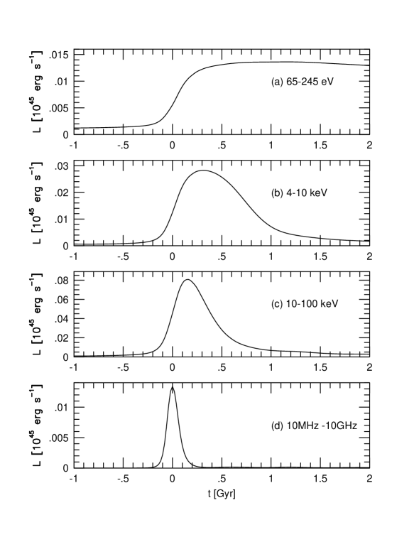
Figure 1: The time evolution of non-thermal emission for various energy band: from top to bottom, inverse Compton scattering of EUVE band (65-245 eV), soft X-ray band (4-10 keV), and hard X-ray band (10-100 keV), and synchrotron radio emission (10 MHz - 10 GHz). The times are relative to the most contracting epoch.

Figure 1 shows the time evolution of non-thermal emission for various energy band: from top to bottom, IC emission of the Extreme Ultraviolet Explorer (EUVE) band (65-245 eV), soft X-ray band (4-10 keV), and hard X-ray band (10-100 keV), and synchrotron radio emission (10 MHz - 10 GHz). The times are relative to the most contracting epoch. The calculation of the luminosity for each band is performed in the simplified assumption that electrons radiate at a monochromatic energy given by $E_{\rm X}=2.5{\rm keV}(E_{\rm e}/{\rm GeV})^{2}$ and $\nu=3.7{\rm MHz}(B/\mu{\rm G})(E_{\rm e}/{\rm GeV})^{2}$ for IC scattering and synchrotron emission, respectively. Since cooling time is roughly proportional to $E_{\rm e}^{-1}$ in these energy range, the higher the radiation energy of IC emission is, the shorter duration of luminosity increase is. In other words, luminosity maximum comes later for lower energy band. Hard X-ray and radio emissions come from the electrons with almost the same energy range. The luminosity maximum in the hard X-ray band, however, comes slightly after the most contracting epoch. On the other hand, radio emission becomes maximum at most contracting epoch since the change of magnetic field due to the compression and expression plays an more crucial role than the increase of relativistic electrons. In any cases, radio halos and hard X-ray are well associated to merger phenomena. They are observable only when thermal ICM have definite signatures of mergers such as complex temperature structures, non-spherical and elongated morphology, or substructures. Soft X-ray emission, which is observable only in clusters (or groups) with relatively low temperature ($\simeq 1$ keV) ICM, is still luminous in $\sim$ 1 Gyr after the merger. Thus, the association of mergers in this band is weaker than in the hard X-ray band. Moreover, EUV emission continues to be luminous after the signatures of the merger have been disappeared in the thermal ICM.

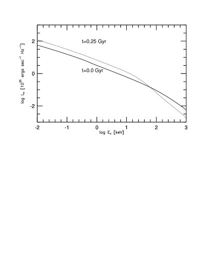
Figure 2: The inverse Compton scattering spectra at $t=0.0$ (solid lines) and $0.25$ (dotted lines).

Figure 2 shows the IC spectra at $t=0.0$ (solid lines) and $0.25$ (dotted lines). In lower energies, $L_{\nu}\propto\nu^{-0.7}$, which is originated from the electron source spectrum $Q(E_{\rm e})\propto E_{\rm e}^{-2.4}$. On the other hand, in higher energies, the spectrums become close to steady solution, $L_{\nu}\propto\nu^{-1.2}$, owing to the IC and synchrotron losses (Longair 1994). The break point of the spectrum moves toward lower energies as time proceeds.

Figure 3 shows the snapshots of synchrotron radio (10MHz-10GHz) surface brightness distribution (solid contours) and X-ray one of thermal ICM (dashed contours) seen from the direction perpendicular to the collision axis. Contours are equally spaced on a logarithmic scale and separated by a factor of 7.4 and 20.1 for radio and X-ray maps, respectively. At $t=-0.25$, the main shocks are located between the two X-ray peaks and relativistic electrons are abundant there. Thus, the radio emission peak is located between the two X-ray peaks although the magnetic field strength there is weaker. At $t=0.0$, relativistic electrons are concentrated around the central region since the main shocks are nearly standing and located near $X\simeq\pm 0.2$. Furthermore, gas infall compress ICM and the magnetic field. Thus, radio distribution shows rather strong concentration. In these phase (at $t=-0.25$ and $0.0$), the radio halo is located at the high temperature region of ICM. On the other hand, at $t=0.25$, relativistic electron distribution becomes rather diffuse since fresh relativistic electrons are producing in the outer regions as the shock waves propagate outwards. At $t=0.25$ the main shocks are located at $X\simeq\pm 1$. Between the shock fronts rather diffuse radio emission is seen. In this phase, the radio halo is located between two high temperature regions of ICM.

As described above, the morphology of the radio halo is strongly depending on the phase of the merger when viewed from the direction perpendicular to the collision axis. When viewed nearly along the collision axis, however, this is not the case. Figure 4 shows the same as figure 3, but for seen from the direction tilted at an angle of $30^{\circ}$ with respect to the collision axis. Radio and X-ray morphology are similar each other in all phases. When the cluster is viewed along the collision axis, the distribution of relativistic electrons roughly follows that of the thermal ICM since the shock fronts face to the observers and spread over the cluster. The distribution of magnetic field strength also roughly follows that of the thermal ICM. Therefor, the radio morphology follows X-ray one.

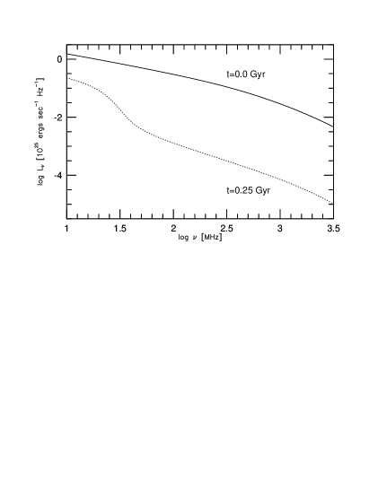
Figure 5: The synchrotron radiation spectra at $t=0.0$ (solid lines) and $0.25$ (dotted lines).

Figure 5 shows the synchrotron radiation spectra at $t=0.0$ (solid lines) and $0.25$ (dotted lines). At $t=0.0$, the synchrotron spectrum follows that of IC emission. On the other hand, at $t=0.25$ there exits a bump at lower energies in the spectrum, which cannot be seen in that of IC emission. Emissivity of synchrotron radiation depends on not only relativistic electron density but also magnetic energy density, which is larger in the central region in this model. On the other hand, IC emissivity depends on the electron density and CMB energy density, which is homogeneous. Thus, the total synchrotron spectrum is more like that in the central region than the total IC spectrum. At $t=0.0$, since relativistic electrons are centered, the emission from the outer region is negligible for both spectra. Thus, similar results are given. On the other hand, at $t=0.25$, propagation of shocks makes a diffuse distribution of relativistic electrons. Therefor, the contribution from the outer region is not negligible for the total IC spectrum while the total synchrotron spectrum is still biased the central region as seen in figure 3. In the central region, however, electrons produced by the main shocks at $t\simeq 0$ with energies more than $\sim$ several GeVs have already cooled down. Thus the spectrum in the central region have a bump in lower energies, which is present in the total spectrum. The emission above $\sim 30$ MHz is mainly due to the electrons produced by the sub-shocks there. If such sub-shocks do not exist, the emission near the main shocks, where the magnetic field strength is rather weaker, can be seen in this energy range. Note that this feature of the synchrotron spectrum is sensitive to the spatial distribution of magnetic field.

5 CONCLUSIONS AND DISCUSSION

We have investigated evolution of non-thermal emission from relativistic electrons accelerated at around the shock fronts during merger of clusters of galaxies. Hard X-ray and radio radiations are luminous only while merger signatures are left in thermal ICM. Hard X-ray radiation becomes maximum in the later stage of merger. In our simulation, radio emission is the most luminous at the most contracting epoch. This is due to the magnetic field amplification by compression. According to the recent magnetohydrodynamical simulations (Roettiger, Stone, & Burns 1999), however, it is possible that the field amplification occurs as the bulk flow is replaced by turbulent motion in the later stages of merger. If this is effective in real clusters, radio emission can increase by a factor of two or three than our results in the later stages of merger. EUV emission is still luminous after the merger signatures have been disappeared in thermal ICM. This is consistent with the EUVE results.

Morphological relation between radio halos and ICM hot regions is described as follows. In the contracting phase, radio halos are located at the hot regions of thermal ICM, or between two substructures (see the left panel of figure 3). This may correspond to A2256 (Röttgering et al. 1994). In the expanding phase, on the other hand, radio halos are located between the two hot regions of ICM and show rather diffuse distribution (see the right panel of figure 3). This may correspond to Coma (Giovannini et al. 1993; Deiss et al. 1997) and A2319 (Feretti, Giovannini, & Böhringer 1997). In the further later phase, the shock fronts reach outer regions and the GeV electrons are already cooled in the central parts. Then, radio halos are located in the cluster outer regions near the shock fronts and we cannot detect radio emission in the central part of the cluster. However, observational correlation between ICM hot regions and radio halos is not clear since the electron temperature there is significantly lower than the plasma mean temperature due to the relatively long relaxation time between ions and electrons (Takizawa 1999, 2000). Note that until now we could only find the electron temperature through X-ray observations. This may correspond to A3667 (Röttgering et al. 1997). It is possible that such radio ‘halos’ located in the outer regions are classified into radio ‘relics’ since their radio powers and spatial scales becomes weaker and smaller than those of typical radio halos, respectively. When the cluster is viewed nearly along the collision axis, however, such morphological relations between radio halo and ICM are unclear and radio and X-ray distributions become similar each other.

We neglect the changes of the spectral index in the electron source term. Since the mach number is gradually increasing as merger proceeds (Takizawa 1999), the spectrum of relativistic electrons becomes flatter as time proceeds. We believe that such changes in the spectral index does not influence our results seriously because most of relativistic electrons are produced in the central high density region, where the mach number is almost constant. In the later stage of merger, however, contribution of relativistic electrons produced in the outer region cannot be negligible in higher energy range ($\sim 10$ GeV) since cooling time is relatively short. Thus, it is probable that the inverse Compton spectrum in the hard X-ray ($\sim 10-100$ keV) becomes flatter in the later stages.

The lower energy part of the electron spectrum can emit hard X-ray through bremsstrahlung. Whether IC scattering or bremsstrahlung is dominant in the hard X-ray range is depending on the shape of the electron spectrum. Roughly speaking, when the spectrum of relativistic electrons is flatter than $E_{\rm e}^{-2.5}$, IC scattering dominates the other and vice versa (see Appendix). Furthermore, the shape of the electron spectrum in the lower energy part is flatter than the originally injected form since the cooling time due to the coulomb loss is proportional to $E_{\rm e}$ and very short (Sarazin 1999). In the present simulation, therefor, it is most likely that the contribution of the bremsstrahlung components in the hard X-ray range is negligible. More detailed calculations, including nonlinear effects for the shock acceleration (Jones & Ellison 1991), by Sarazin & Kempner (1999) show that IC scattering is dominant in the hard X-ray when the accelerated electron momentum spectrum is flatter than $p_{\rm e}^{-2.7}$, which corresponds to the electron energy spectrum of $E_{\rm e}^{-2.7}$ in the fully relativistic range. Thus, the bremsstrahlung contribution in the hard X-ray should be considered in mergers with low mach numbers.

A merger shock acceleration model also predicts some gamma-ray emission. Electrons which radiate EUV due to IC scattering also emit $\sim 100$ MeV gamma-ray through bremsstrahlung. Furthermore, it is most likely that protons as well as electrons are accelerated at around the shock fronts. Such high energy protons also produce gamma-rays peaked at $\sim 100$ MeV through decay of neutral pions. Although the energy density ratio between electrons and protons in acceleration site is uncertain, the contributions of protons and the bremsstrahlung to the emission become important in the higher energies. We think that it is interesting to investigate from hundreds MeV to multi TeV emissions, which are observable with operating instruments such as EGRET, ground-based air Čerenkov telescopes, and planning projects like GLAST satellites. However, since the diffusion length of protons within the cooling time is much longer than that of electrons, treatment of the diffusion-loss equation for protons are more complex than the model in this paper.

Appendix A ESTIMATION OF THE BREMSSTRAHLUNG CONTRIBUTION IN THE HARD X-RAY RANGE

We estimate the contribution of the bremsstrahlung form the lower energy part of the electron spectrum to the hard X-ray emission in our model, which is neglected in this paper. Although the crude estimations discussed here are order-of magnitudes, it is helpful to explain which mechanism, IC scattering and bremsstrahlung radiation, is dominant.

The standard theory of 1st order Fermi acceleration provides power law spectrum in momentum distribution. We, therefore, assume the momentum spectrum of accelerated electrons has a form of

$$\frac{dN_{\rm e}}{dP_{\rm e}}=cN_{\rm 0}\left(\frac{P_{\rm e}}{m_{\rm e}c}\right)^{-\alpha}\ \ {\rm[cm^{-3}\ (eV\ {\mit c}^{-1})^{-1}]}\ ,$$ (A1)

where $P_{\rm e}$ is an electron momentum, $c$ is the speed of light, and $m_{\rm e}$ is the electron rest mass. Using the relation between the momentum $P_{\rm e}$ and the kinetic energy $E_{\rm e}$, $E_{\rm e}=(P_{\rm e}^{2}c^{2}+m_{\rm e}^{2}c^{4})^{1/2}-m_{\rm e}c^{2}$, the spectrum for kinetic energy is given by

$$\frac{dN_{\rm e}}{dE_{\rm e}}=N_{\rm 0}\frac{E_{\rm e}+m_{\rm e}c^{2}}{m_{\rm e}c^{2}}\left(\frac{P_{\rm e}}{m_{\rm e}c}\right)^{-\alpha-1}\ \ {\rm[cm^{-3}\ (eV)^{-1}]}\ .$$ (A2)

For relativistic electrons, $E_{\rm e}\gg m_{\rm e}c^{2}$, the spectrum becomes

$$\frac{dN_{\rm e}}{dE_{\rm e}}=N_{\rm 0}\left(\frac{E_{\rm e}}{m_{\rm e}c^{2}}\right)^{-\alpha}\ ,$$ (A3)

which is consistent with an assumption of $Q(E_{\rm e},t)$ in section 3. Since the hard X-ray photons are produced from CMB photon field via IC scattering of relativistic electrons in our model, we use this form for the estimation of IC emissivity. For non-relativistic electrons, $E_{\rm e}\ll m_{\rm e}c^{2}$, the spectrum becomes

$$\frac{dN_{\rm e}}{dE_{\rm e}}=2^{-\frac{\alpha+1}{2}}N_{\rm 0}\frac{E_{\rm e}+m_{\rm e}c^{2}}{m_{\rm e}c^{2}}\left(\frac{E_{\rm e}}{m_{\rm e}c^{2}}\right)^{-\frac{\alpha+1}{2}}\ ,$$ (A4)

where we use the relation $E_{\rm e}=P_{\rm e}^{2}/(2m_{\rm e})$. Since the bremsstrahlung radiation at the hard X-ray range is emanated from electrons with almost the same energy range, we use this form for the estimation of bremsstrahlung emissivity.

For simplicity, we approximate the emissivity, $\epsilon$, for both IC and bremsstrahlung processes to be,

$$\epsilon={\frac{dN_{\rm e}}{dE_{\rm e}}}\frac{dE_{\rm e}}{d{\varepsilon}_{\rm\gamma}}{\left|\frac{dE_{\rm e}}{dt}\right|}\ \ {\rm[erg\ s^{-1}\ cm^{-3}\ eV^{-1}]}\ ,$$ (A5)

where the emission rate is assumed to be equal to the electron energy loss rate and $\varepsilon_{\gamma}$ is the photon energy.

To obtain the bremsstrahlung emissivity, we assume that an electron with energy $E_{\rm e}$ loses its energy to emit photon of energy $\varepsilon_{\rm\gamma}=E_{\rm e}$ after it has traversed one mean free path $X_{\rm 0}$. Hence,

$$\frac{dE_{\rm e}}{d{\varepsilon}_{\rm\gamma}}=1,$$ (A6)

and

$$\left|\frac{dE_{\rm e}}{dt}\right|\sim\varepsilon_{\rm\gamma}\frac{v_{\rm e}}{X_{\rm 0}}\ \ {\rm[erg\ s^{-1}]}\ ,$$ (A7)

where $v_{\rm e}$ is electron velocity. From $\sigma_{\rm T}n_{\rm 0}X_{\rm 0}\sim 1$, we approximate

$$\left|\frac{dE_{\rm e}}{dt}\right|\sim\varepsilon_{\rm\gamma}v_{\rm e}\sigma_{\rm T}n_{\rm 0}\ ,$$ (A8)

where $\sigma_{\rm T}$ denotes the cross section of Thomson scattering and $n_{\rm 0}$ denotes the density of ambient matter. Using equations (A4), (A5), (A6), and (A8), we estimate the bremsstrahlung emissivity in the hard X-ray energy range, $\varepsilon_{\rm\gamma}=\varepsilon_{\rm HXR}$, as

$$\epsilon_{\rm brem}\sim 2^{-\frac{\alpha}{2}}N_{\rm 0}\sigma_{\rm T}cn_{\rm 0}m_{\rm e}c^{2}\left(1+\frac{\varepsilon_{\rm HXR}}{m_{\rm e}c^{2}}\right)\left(\frac{\varepsilon_{\rm HXR}}{m_{\rm e}c^{2}}\right)^{-\frac{\alpha}{2}+1}\ ,$$ (A9)

For IC scattering of CMB photons, the photon energy after the scattering by an electron with energy $E_{\rm e}=m_{\rm e}\gamma_{\rm e}c^{2}$ is approximated by single energy of $\varepsilon_{\rm\gamma}={\gamma_{\rm e}}^{2}\bar{\varepsilon}_{\rm CMB}$, where $\bar{\varepsilon}_{\rm CMB}$ is peak energy of CMB spectrum. Thus,

$$\frac{dE_{\rm e}}{d{\varepsilon}_{\rm\gamma}}=\frac{1}{2}\left(\frac{\bar{\varepsilon}_{\rm CMB}}{m_{\rm e}c^{2}}\right)^{-\frac{1}{2}}\left(\frac{\varepsilon_{\rm\gamma}}{m_{\rm e}c^{2}}\right)^{-\frac{1}{2}}\ .$$ (A10)

Since the scattering is in Thomson energy range ($\bar{\varepsilon}_{\rm CMB}\gamma_{\rm e}\gg m_{\rm e}c^{2}$), we set

$$\left|\frac{dE_{\rm e}}{dt}\right|=\frac{4}{3}\sigma_{\rm T}c{\gamma_{\rm e}}^{2}\bar{\varepsilon}_{\rm CMB}n_{\rm CMB}\ \ {\rm[erg\ s^{-1}]}\ ,$$ (A11)

where $n_{\rm CMB}$ is photon number density of CMB fields. Using equations (A3), (A5), (A10), and (A11), we estimate the IC emissivity in the hard X-ray energy range, $\varepsilon_{\rm\gamma}=\varepsilon_{\rm HXR}$, as

$$\epsilon_{\rm IC}=\frac{2}{3}N_{\rm 0}\sigma_{\rm T}c\bar{\varepsilon}_{\rm CMB}n_{\rm CMB}\left(\frac{\bar{\varepsilon}_{\rm CMB}}{m_{\rm e}c^{2}}\right)^{\frac{\alpha-3}{2}}\left(\frac{\varepsilon_{\rm HXR}}{m_{\rm e}c^{2}}\right)^{-\frac{\alpha-1}{2}}\ .$$ (A12)

From equations (A9) and (A12), we derive the emissivity ratio as

$$\frac{\epsilon_{\rm brem}}{\epsilon_{\rm IC}}=\frac{3}{2}\frac{n_{\rm 0}}{n_{\rm CMB}}\left(1+\frac{\varepsilon_{\rm HXR}}{m_{\rm e}c^{2}}\right)\left(\frac{\bar{\varepsilon}_{\rm CMB}}{m_{\rm e}c^{2}}\right)^{\frac{1}{2}}\left(\frac{\varepsilon_{\rm HXR}}{m_{\rm e}c^{2}}\right)^{\frac{1}{2}}\left(2\frac{\bar{\varepsilon}_{\rm CMB}}{m_{\rm e}c^{2}}\right)^{-\frac{\alpha}{2}}\ .$$ (A13)

For $\epsilon_{\rm brem}<\epsilon_{\rm IC}$, we get the relation

$$\alpha<\frac{2\ln\left[\frac{3}{2}\frac{n_{\rm 0}}{n_{\rm CMB}}\left(1+\frac{\varepsilon_{\rm HXR}}{m_{\rm e}c^{2}}\right)\frac{(\bar{\varepsilon}_{\rm CMB}\varepsilon_{\rm HXR})^{\frac{1}{2}}}{m_{\rm e}c^{2}}\right]}{\ln\left(\frac{2\bar{\varepsilon}_{\rm CMB}}{m_{\rm e}c^{2}}\right)}\ .$$ (A14)

Substituting typical values for ICM at $z\sim 0$, $n_{\rm 0}=1\times 10^{-3}\ \ {\rm cm^{-3}}$, $n_{\rm CMB}=400\ \ {\rm cm^{-3}}$, $\bar{\varepsilon}_{\rm CMB}=6.57\times 10^{-4}\ \ {\rm eV}$, and $\varepsilon_{\rm HXR}=10\ \ {\rm keV}$, we obtain $\alpha<2.5$. At $\varepsilon_{\rm HXR}=100\ \ {\rm keV}$, the spectrum of equation (A9) becomes steeper as electrons enter the trans-relativistic energy range. As a result, the bremsstrahlung emissivity is reduced so that the larger index of electron spectrum is accepted for $\epsilon_{\rm brem}<\epsilon_{\rm IC}$.

Figure 3: Snapshots of synchrotron radio (10MHz-10GHz) surface brightness distribution (solid contours) and X-ray one of thermal ICM (dashed contours) seen from the direction perpendicular to the collision axis. Contours are equally spaced on a logarithmic scale and separated by a factor of 7.4 and 20.1 for radio and X-ray maps, respectively.

Figure 4: Same as figure 3, but for seen from the direction tilted at an angle of $30^{\circ}$ with respect to the collision axis.

References

- (1) Blasi, P. & Colafrancesco, S. 1999, Astrop. Phys., 12, 169
- (2) Deiss, B. M., Reich, W., Lesch, H., Wielebinski, R. 1997, A&A, 321, 55
- (3) Dennison, B. 1980, ApJ, 239, L93
- (4) Drury, L. O’C. 1983, Rep. Prob. Phys., 46, 973
- (5) Feretti, L., Giovannini, G. & Böhringer, H. 1997, New Astronomy, 2, 501
- (6) Fukazawa, Y. 1999, in Proc. ASCA Symposium on Heating and Acceleration in the Universe, ed. H. Inoue, T. Ohashi, & T. Takahashi, in press
- (7) Fusco-Femiano, R., Fiume, D. D., Feretti, L., Giovannini, G., Grandi, P., Matt, G., Molendi, S., and Santangelo, A. 1999, ApJ, 513, L21
- (8) Giovannini, G., Feretti, L., Venturi, T., Kim, K. T., and Kronberg, P. P. 1993, ApJ, 406, 399
- (9) Henriksen, M. J., & Markevitch, M. 1996, ApJ, 466, L79
- (10) Honda, H., Hirayama, M., Watanabe, M., Kunieda, H., Tawara, Y., Yamashita, K., Ohashi, T., Hughs, J., P., & Henry, J. P. 1996, ApJ, 473, L71
- (11) Ishizaka, C., & Mineshige, S. 1996, PASJ, 48, L37
- (12) Jones, F. C., & Ellison, D. C. 1991, Space Sci. Rev., 58, 259
- (13) Kaastra, J. S., Lieu, R., Mittaz, J. P. D., Bleeker, J. A. M., Mewe, R., Colafrancesco, S., & Lockman, F. J. 1999, ApJ, 519, L119
- (14) Lieu, R., Mittaz, J. P. D., Bowyer, S., Lockman, F. J., Hwang, C.-Y., & Schmitt, J. H. M. M. 1996 ApJ, 458, L5.
- (15) Lieu, R., Bonamente, M., & Mittaz, J. P. D. 1999, ApJ, 517, L91
- (16) Longair, M. S. 1994, High Energy Astrophysics (Cambridge: Cambridge University Press)
- (17) Mittaz, J. P. D., Lieu, R., & Lockman, F. J. 1998, ApJ, 498, L17
- (18) Markevitch, M., Sarazin, C. L., & Vikhlinin, A. 1999, ApJ, 521, 526
- (19) Monaghan, J. J. 1992, ARA&A, 30, 543
- (20) Naito, T., Yoshida, T., Mori, M. and Tanimori, T., in Proc. ASCA Symposium on Heating and Acceleration in the Universe, ed. H. Inoue, T. Ohashi, & T. Takahashi, in press.
- (21) Rephaeli, Y. 1979, ApJ, 227, 364
- (22) Rephaeli, Y., Gruber, D., & Blanco, P. 1999, ApJ, 511, L21
- (23) Roettiger, K., Stone, J. M., & Burns, J. O. 1999, ApJ, 518, 594
- (24) Roettiger, K., Burns, J. O., & Stone, J. M. 1999, ApJ, 518, 603
- (25) Röttgering, H., Snellen, I., Miley, G., de Jong, P., Hanisch, R. J., & Perley, R. 1994, ApJ, 436, 654
- (26) Röttgering, H. J. A., Wieringa, M. H., Hunstead, R. W., and Ekers, R. D. 1997, MNRAS, 290, 577
- (27) Sarazin, C. L. 1999, ApJ, 520, 529
- (28) Sarazin, C. L., & Kempner, J. C. 1999, ApJ, in press, astro-ph/9911335
- (29) Schindler, S., & Müller, E. 1993, A&A, 272, 137
- (30) Takizawa, M. 1999, ApJ, 520, 514
- (31) Takizawa, M. 2000, ApJ, in press, astro-ph/9910441
- (32) Tanimori, T. et al. 1998, ApJ, 497, L25
- (33) Watanabe, M., Yamashita, K., Furuzawa, A., Kunieda, H., Tawara, Y., & Honda, H. 1999, ApJ, in press