[

Globally coupled bistable elements as a model of group decision making

Abstract

A simple mathematical model is proposed to study the effect of the average trend of a population on the opinion of each individual, when a group decision has to be made by voting. It is shown that if such effect is strong enough a transition to coherent behavior occurs, in which the whole population converges to a single opinion. This transition has the character of a first-order critical phenomenon.

]

Group decision making is a complex social process in which the inherent factors that determine the position of each individual –such as previous experience, prospective benefits, current personal circumstances, and character– interact in a nontrivial way with the average trend, to which individuals are exposed through communication between them. Group decision results from this interaction as an emerging property of their collective behavior.

Consider as a specific case an ensemble of individuals that have to choose, at a given time in the future and by individual voting, and option among a prescribed set of instances. After vote counting, the decision is simply taken for the most voted option. This decision –which, once votes have been emitted, is straightforwardly defined– results however from the complex collective process that builds up the opinion of each individual [1]. During a certain period previous to the voting act, in fact, the opinion of a given individual evolves due to the modulation that the knowledge of another’s position imposes on the own tendency. In an efficiently communicating ensemble, like in any modern population, individuals are continuously exposed to the average opinion of the ensemble –for instance, through poll results, published by mass communication media– and are expected to be more or less strongly influenced by this collective element [2].

This paper is aimed at exploring, in the frame of a simple mathematical model, how the effects of the personal trend and of the average opinion in defining the individual vote combine with each other to lead the group to its collective decision. For the sake of concreteness, suppose that the population has to choose by voting among two candidates, $C^{+}$ and $C^{-}$. In the model, the time evolution of the opinion of the $i$-th individual is described by a variable $x_{i}(t)$, with $x_{i}\in[-1,1]$ for all $i$ and $t$. Large values of $x_{i}$, $|x_{i}|\approx 1$, are to be associated with a firm decision to vote for one of the two candidates, ($C^{+}$ for $x_{i}>0$ and $C^{-}$ for $x_{i}<0$, say), whereas small values of $x_{i}$ correspond to a looser opinion. In any case, when the voting act takes place the individual opinion is quenched and the decision is made according to the sign of $x_{i}$ at that time. In practice, it is supposed that the typical evolution times for the individual opinion are shorter than the time elapsed up to the voting act, so that one will focus the attention on the long-time asymptotics of the model.

The average opinion, which is expected to play a relevant role in the definition of the individual decision, is here characterized by the arithmetic mean value

$$\bar{x}(t)=\frac{1}{N}\sum_{i}x_{i}(t),$$ (1)

where $N$ is the size of the population. This mean value is a measure of how much defined is the global trend towards on the two candidates. In fact, the sign of $\bar{x}$ at the time of the voting act determines the chosen candidate.

To stress the effect of the average opinion on the individual vote it is assumed that, in the absence of such effect, each individual would simply reinforce his or her initial personal opinion as time elapses. This means, in particular, that a given individual would not change his or her original preference for one of the candidates. This behavior is well represented by the following dynamical equation for $x_{i}(t)$:

$$\frac{dx_{i}}{dt}=x_{i}-x_{i}^{3}\ \ \ \ \ (i=1,2,\dots,N).$$ (2)

In fact, the solution to this equation approaches the asymptotic value $x_{i}(\infty)=+1$ or $x_{i}(\infty)=-1$ depending on the initial value $x_{i}(0)$ being positive or negative, respectively. Moreover, $x_{i}(t)$ does not change its sign during the whole evolution. If $x_{i}(0)=0$, then $x_{i}(t)=0$ for all $t$, but this stationary state is unstable. These facts can readily be verified from the explicit solution to Eq. (2), which reads,

$$x_{i}(t)=\frac{x_{i}(0)}{\sqrt{x_{i}(0)^{2}-[x_{i}(0)^{2}-1]\exp(-2t)}}.$$ (3)

From a dynamical viewpoint, Eq. (2) implies that each individual behaves as a bistable element, its asymptotic state being fixed by the initial condition. In physics, this kind of model has been used to study spin systems (in the soft-spin approximation) [3] and neural networks [4].

The effect of the average opinion on the evolution of the individual trend is described by modifying Eq. (2) in the following way:

$$\frac{dx_{i}}{dt}=x_{i}-x_{i}^{3}+k_{i}(\bar{x}-x_{i})\ \ \ \ \ (i=1,2,\dots,N),$$ (4)

where $\bar{x}(t)$ has been defined in (1) and $k_{i}$ is a constant that, as discussed in the following, measures the influence of the average opinion on the $i$-th individual. For $k_{i}>0$ the new terms drive $x_{i}(t)$ towards the average $\bar{x}(t)$. In fact, for large values of $k_{i}$ and slowly varying $\bar{x}$, the individual variable $x_{i}$ would exponentially approach the average. The new terms thus represent, for positive $k_{i}$, a trend of the $i$-th individual to follow the average opinion, which can either reinforce or compete with his or her individual position. Negative values of $k_{i}$ would correspond to individuals who tend to take a position opposite to the average.

In a physical context, the new terms represent an “interaction” between individuals. From a mathematical viepoint, in fact, those terms couple the set of equations (4) through the average $\bar{x}$, which depends on the whole set of $x_{i}$ $(i=1,\dots,N)$. This coupling makes it impossible to give the exact solution to the model equations (4), and the system has to be treated numerically. In particular, note that it is not possible to derive an autonomous equation for the evolution of the average $\bar{x}(t)$.

The case where the coupling constant $k_{i}$ is positive and the same for all individuals, $k_{i}=k>0$ for all $i$, is considered first. Obviously, for $k=0$ the uncoupled ensemble –whose behavior has been discussed above– is recovered. For $k=1$, Eq. (4) reduces to

$$\frac{dx_{i}}{dt}=\bar{x}-x_{i}^{3}.$$ (5)

Let $r_{ij}=x_{i}-x_{j}$ be the difference between the states of any two individuals. It can be shown from Eq. (5) that, if $-1<x_{i},x_{j}<1$, $r_{ij}$ tends to zero as time elapses [5]. In other words, for $k=1$ the model predicts that all the individuals will have the same opinion at sufficiently long times.

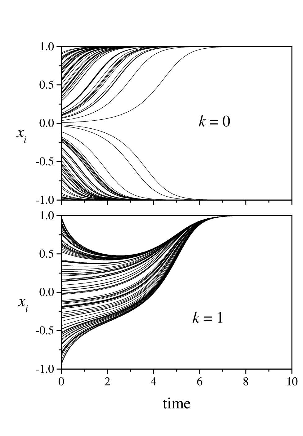
FIG. 1.: Evolution of $x_{i}$ for a population of 1000 individuals with $k=0$ and $k=1$. For clarity, only 100 states are displayed. The initial distribution is uniform over $[-1,1]$.

Figure 1 shows the evolution of $x_{i}$ in a population of 1000 individuals for $k=0$ and $k=1$. For the sake of clarity, only 100 variables are displayed. Initially, the individual states are randomly distributed in $[-1,1]$. As expected, for $k=0$ the states are soon divided into two clusters, according to their signs. For $k=1$, instead, all states are attracted to a single cluster. Since for this value of the coupling constant the average opinion is already dominant and all the individuals behave in a coherent way, it can be predicted that for $k>1$ the dynamics of the ensemble is qualitatively the same. This is indeed verified from numerical results. On the other hand, for $0<k<1$ a transition is expected to occur between the two qualitative different behaviors observed at $k=0$ and $k=1$. This transition is characterized in the following.

According to numerical calculations, for sufficiently small values of the coupling constant the collective behavior qualitatively reproduces the evolution of the uncoupled ensemble ($k=0$). In fact, if the initial distribution of $x_{i}$ is uniform over $[-1,1]$ the population becomes divided into two groups –as when, for $k=0$, both signs are initially present. If, instead, one of the signs is much more abundant than the other, all the variables may ultimately converge to one of the extreme values $x_{i}=\pm 1$ –as when, for $k=0$ only one sign is initially present. The interacting ensemble is therefore “bistable,” in the sense that two qualitatively different asymptotic states are observed depending on the initial condition: either all individuals behave coherently, or they become divided into two groups. On the other hand, as stated above, for larger values of $k$ only coherent behavior is observed. Figure 2 illustrates these behaviors for intermediate values of $k$.

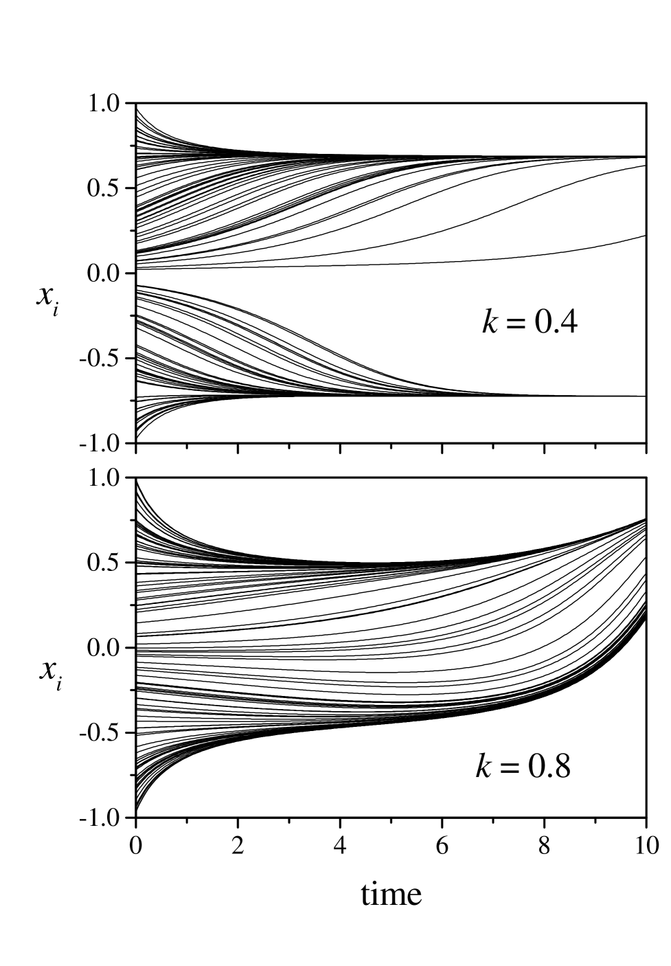
FIG. 2.: Evolution of $x_{i}$ for a population of 1000 individuals with $k=0.4$ and $k=0.8$. For clarity, only 100 states are displayed. The initial distribution is uniform over $[-1,1]$.

The transition between bistable and coherent behavior is due to a stability change in the possible asymptotic states of the coupled ensemble. Suppose that, as the system evolves, the $N$ individuals become divided into two groups. One of them, with $pN$ individuals ($0\leq p\leq 1$) approaches the asymptotic state $X_{1}$, whereas the other, with $(1-p)N$ individuals, approaches $X_{2}$. It has to be stressed that the value of $p$ depends in a nontrivial way on the initial condition, and cannot be analytically determined a priori. According to Eq. (4) the following identities should hold for $t\to\infty$ and $N\to\infty$:

$$\begin{array}[]{rl}0&=(1-k)X_{1}+k[pX_{1}+(1-p)X_{2}]-X_{1}^{3}\\ \\ 0&=(1-k)X_{2}+k[pX_{1}+(1-p)X_{2}]-X_{2}^{3}.\end{array}$$ (6)

These equations include also the case of coherent behavior, if one puts $X_{1}=X_{2}$ with any value of $p$. Their solutions constitute the set of stationary states for the system, whose stability can be studied by means of standard linearization around equilibria.

Equations (6) can be reduced to a 9th-degree polynomial equation for either $X_{1}$ or $X_{2}$, and have therefore nine solutions –which in general are complex numbers. The trivial solution $X_{1}=X_{2}=0$ is unstable. The remaining eight solutions can be grouped into symmetrical pairs, ($X_{1},X_{2}$) and ($-X_{1},-X_{2}$), both with the same stability properties. It is therefore enough to analyze, for instance, the four solutions with $X_{1}\geq 0$. (i) The first one, $X_{1}=X_{2}=1$, is stable for all $k$ and corresponds to the asymptotic state of coherent evolution. (ii) The second solution is real and unstable for all $k$. It approaches the unstable solution $(0,-1)$ for $k\to 0$ and the trivial solution for $k\to 1$. (iii) Another unstable solution approaches the unstable state ($0,1$) as $k\to 0$. (iv) Finally, there is a stable solution that approaches $(1,-1)$ as $k\to 0$. This solution corresponds to the case where the individuals have become divided into two groups.

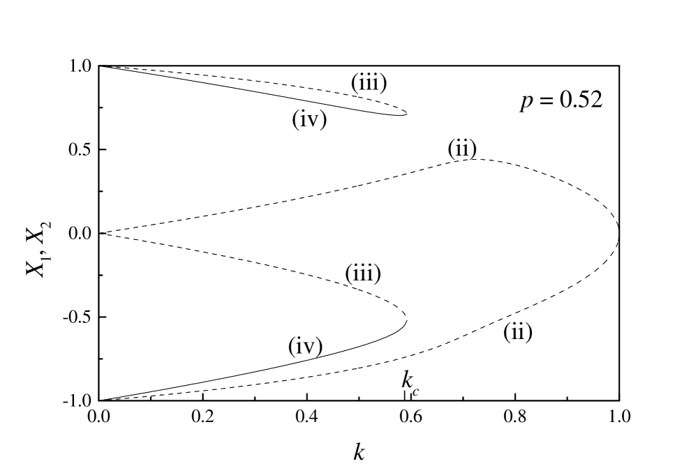
FIG. 3.: The equilibrium states $X_{1}$ and $X_{2}$ as a function of $k$ for solutions (ii), (iii), and (iv) (see text), at $p=0.52$. For the solutions displayed, $X_{1}$ is always positive and $X_{2}$ is always negative.

Figure 3 shows the numerical results for $X_{1}$ and $X_{2}$ as a function of $k$, for $p=0.52$. Solid lines indicate stable solutions whereas dashed lines stand for unstable solutions. As the coupling constant grows, there is a critical value $k_{c}$ at which the two solutions (iii) and (iv) collide and become complex. At this critical value, the solution where the population is divided into two groups dissapears. The value of $k_{c}$ is related to $p$ by the following polynomial equation:

$$4k_{c}-18k_{c}^{2}(p-p^{2})+27k_{c}^{4}(p^{2}-2p^{3}+p^{4})=1.$$ (7)

Thus, for a given value of $p$ –which is determined by the initial condition– and $k<k_{c}$, two qualitatively different behaviors can occur. Either $X_{1}=X_{2}=\pm 1$, and the system evolves coherently, or $X_{2}\neq X_{1}$, and the individuals are divided into two groups. For $k>k_{c}$, instead, only coherent behavior is possible. Thus, for sufficiently large $k$, the opinion of the whole population approaches the same state. Figure 4 shows a phase diagram $k$ versus $p$, where the boundary between the zones of bistability and coherence given by Eq. (7) is shown.

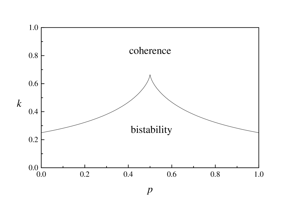
FIG. 4.: Phase diagram in the ($p,k$) plane, displaying the zones of coherent behavior and bistability.

The transition between bistability and coherence can be characterized by a single order parameter introducing, for instance, the mean difference $\delta$ between the states of any pair of individuals,

$$\delta=\frac{1}{2}p(1-p)|X_{1}-X_{2}|,$$ (8)

which has been plotted in Fig. 5 as a function of $k$ for $p=0.52$. The dependence of $\delta$ on the coupling constant suggests classifying the transition as a first-order critical phenomenon.

Naturally, the assumption that all the individuals in the population are equally influenced by the average opinion –i.e. that all the individuals have the same coupling constant $k$– is not a very realistic one. Rather, it is to be expected that the coupling constants are distributed within a certain interval, with some individuals being more influenced by another’s opinion than other. It could moreover be supposed that some individuals are negatively affected by the mean trend, tending to make their own opinion diverging from the average. This case would correspond to $k_{i}<0$.

In this case of inhomogeneous behavior it can be easily shown from Eq. (4) that the asymptotic state of $x_{i}(t)$ depends on the value of $k_{i}$. This relation is implicitly given by the equation

$$k_{i}=\frac{x_{i}^{3}-x_{i}}{\bar{x}-x_{i}}.$$ (9)

Numerical simulations show however that, as far as the distribution of coupling constants $k_{i}$ is moderately narrow, the qualitative collective behavior is the same as for uniform $k$. Mathematically, it is not an easy task to characterize the situation in which this behavior breaks down as the values of $k_{i}$ become more and more scattered. Is is nevertheless expected that coherent evolution can be destroyed if the coupling constants are sufficiently different from each other, including in particular some negative values. A sufficient condition for coherence to fail is in fact that a single individual has a coupling constant $k_{i}<-2$. In this situation, however, it is this only individual who fails to behave coherently, thus not affecting the result of the collective decision making.

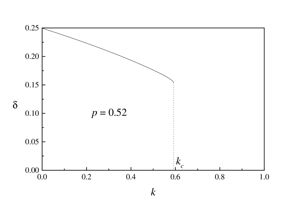
FIG. 5.: The order parameter $\delta$ as a function of $k$, for $p=0.52$. At $k_{c}\approx 0.592$, $\delta$ vanishes suddenly.

In summary, it has been here shown within a simple mathematical model that, under a sufficiently strong influence of the average trend of a population on the opinion of each individual, the population behaves coherently and votes converge towards a single candidate. For weaker coupling between individuals, instead, votes are more evenly divided between the two candidates. The transition between both behaviors is abrupt and, in fact, has the character of a critical phenomenon. This is qualitatively similar to the ferromagnetic phase transition observed in spin systems –though in this physical phenomenon the phase transition is of the second order [6]. Indeed, beyond the critical point the state of all the elements in the system coincide, even in spite of the initial condition corresponding to a uniform distribution of states. The coupling mechanism is in fact able to break the initial macroscopic homogeneity, enhancing microscopic fluctuations. It can be interesting to further analyze this model, including for instance local communication ways between individuals as well as noise, that can perturb in a nontrivial way the properties of the quoted transition [7].

The present results could encourage unfair, unscrupulous candidates to manipulate poll results published in mass media –if they have the power to do so– in their own benefit.

REFERENCES

- [1] B. Berenson, P. Lazarsfeld, and W. McPhee, Voting. A Study of Opinion Formation in a Presidential Campaign (The University of Chicago Press, Chicago, 1954).
- [2] J. Klapper, The Effects of Mass Communication (The Free Press, New York, 1960); E. Katz, The Utilization of Mass Communication by the Individual (Oxford University Press, New York, 1979).
- [3] P. Jung, U. Behn, E. Pantazelou, and F. Moss, Phys. Rev. A 46, R1709 (1992).
- [4] H. Sompolinsky, Phys. Rev. A 34, 2571 (1986); ibid. 37, 4865 (1988).
- [5] D.H. Zanette, Phys. Rev. E 55, 5315 (1997).
- [6] D.L. Goodstein, States of Matter (Dover, New York, 1975).
- [7] N. van Kampen, Stochastic Processes in Physics and Chemistry (North-Holland, Amsterdam, 1992).