A microsimulation of traders activity in the stock market:
the role of heterogeneity, agents’ interactions and trade frictions.

Abstract

We propose a model with heterogeneous interacting traders which can explain some of the stylized facts of stock market returns. In the model, synchronization effects, which generate large fluctuations in returns, can arise purely from communication and imitation among traders. The key element in the model is the introduction of a trade friction which, by responding to price movements, creates a feedback mechanism on future trading and generates volatility clustering. The model also reproduces the empirically observed positive cross-correlation between volatility and trading volume.

JEL classification: G12, C63
Keywords: Volatility clustering, fat tails, trading volume, herd behaviour.

I Introduction

As pointed out by several authors, since Mandelbrot (1963), the probability distributions of returns of many market indices and currencies, over different but relatively short time intervals, display fat tails. It is estimated that the shape of a Gaussian, as predicted by the random-walk hypothesis, is recovered only on longer time scales, i.e. of one month or more. The empirical distribution of returns shows an asymptotic power law decay $P(r)\sim r^{-(1+\mu)}$ with an exponent $2<\mu<4$ (Pagan (1996), Guillaume et al. (1997), Gopikrishnan et al. (1999)).

Moreover, while stock market returns are uncorrelated on lags larger than a single day, the autocorrelation function of the volatility is positive and slowly decaying, indicating long memory effects. This phenomenon is known in the literature as volatility clustering (Ding et al. (1993), de Lima & Crato (1994), Ramsey (1997), Ramsey & Zhang (1997)). Empirical analysis on market indices and exchange rates shows that the volatility autocorrelations are power-laws over a large range of time lags (from one day to one year), in contrast with ARCH-GARCH models (Engle (1995), Bollerslev (1986)) where they are supposed to decay exponentially.

Daily financial time series also provide empirical evidence (Tauchen & Pitts (1983), Ronals et al. (1992), Pagan (1996)) of a positive autocorrelation, with slowly decaying tails, for the trading volume, and positive cross correlation between volatility of returns and trading volume.

There is also some evidence that both the moments of the distribution of returns (Ghashghaie et al. (1996), Baviera et al. (1998)) and the volatility autocorrelations (Baviera et al. (1998), Pasquini & Serva (1998)) display what is termed in the theory of turbulent systems as multiscaling (see section IV for a description of multiscaling).

It is not settled yet whether these power law fluctuations merely reflect the probability distributions of exogenous shocks hitting the market or whether they are related to the inherent interaction among market players and the trading process itself. For example, it is widely believed that stock markets are vulnerable to collective behaviour whereby a large group of agents place the same order simultaneously. This can manifest itself in large price fluctuations, and eventually crashes. Such collective behaviour could reflect the phenomenon known as herding which occurs when agents take actions on the basis of imitating each other (Bannerjee (1992), Bannerjee (1993), Orlean (1995), Cont & Bouchaud (1999)). To model how the decisions of agents are influenced by their mutual interaction, this paper assumes a simple communication structure based on ideas from statistical physics in which agents occupy the nodes of a lattice and are influenced by the decisions of their nearest neighbours. Agents are assumed to be heterogenous in their exposure to a trading friction which can restrict market participation. Heterogeneity ensures that traders do not spontaneously make the same decisions; indeed, this would make superfluous the coordinating role of communication. We pursue the claim that the interactions among traders and their heterogeneous nature by themselves, can help explain the statistical features observed in the financial data. Since the crucial point is not the exact description of individual behaviour but the interrelation between and the statistical differences across agents, our model will be based on noise trading expanded to allow for heterogeneity and communication effects.

A variety of agent-based model have been proposed in the last few years to study financial markets ( Arthur (1997), Caldarelli et al. (1997), Bak et al. (1997), Farmer (1998), LeBaron (1999), Lux and Marchesi (1999), Cont & Bouchaud (1999), Focardi et al. (1999), Stauffer et al. (1999)). Cont and Bouchaud (1999) introduce a model which is similar to the one we use in this paper. One of the differences is that in their model imitation takes the form that agents act in clusters rather than individually. Furthermore, a probability $p$ is associated with a link existing between any two agents and this determines the distribution of cluster sizes. The trading activity of each group is controlled exogenously. For low activity and at a critical value of $p$ the distribution of returns shows a power law behaviour with an exponent $\mu$ which can vary from $1$ to $1.5$ (depending on the dimensionality of the system). This is smaller than the empirically observed value $\mu\sim 3$ which our own model is capable of reproducing. Various mechanisms have been proposed to improve the agreement of the Cont-Bouchaud model with real data. Zhang (1999) suggests a non linear price rule which assumes that price changes are proportional to the square root of the difference between demand and supply. Zhang finds an exponent $\mu=1.9$ for a two dimentional lattice, which is still below the empirical value.

Both the above papers are concerned only with explaining the power-law behaviour of the distribution of returns and not with volatility clustering. In a recent paper, Stauffer and Sornette (1999) consider a modified version of the Cont-Bouchaud model, where the connectivity of the system is changed by slowly adjusting the value of $p$ at each time step. This mechanism produces volatility clustering and a better agreement with the empirical exponent. However, the adjustment of $p$ is entirely exogenous and does not have an underlying economic explanation.

Our model suggests an endogenous mechanism for changing the level of correlation among agents (analogous to changing the connectivity in the above paper) and also endogenizes the exponent of the pricing rule (which is held constant to $1/2$ in Zhang). It provides a better agreement with the stylized facts of stock market dynamics, including cross-correlation between trading volume and volatility which were not addressed by the other authors.

The rest of the paper is organized as follows: the next section describes the model and the simulation strategy, section $3$ discusses results and section $4$ concludes.

II The Model

A modified version of the random field Ising model (RFIM) (Sethna (1993), Galam(1997)) is employed to describe the trading behaviour of agents in a stock market. We consider an $L\times L$ square lattice where each node $i$ represents an agent and the links represent the connections among agents. Each agent is connected to his four nearest neighbours, the ones above, below, left and right. Periodical boundary conditions are adopted so that the agents at the top of the lattice are linked to those at the bottom and the agents at the left side are linked to those at the right side. In this way the lattice assumes the topology of a torus.

We start with each agent initially owning the same amount of capital consisting of two assets: cash $M_{i}(0)$ and $N_{i}(0)$ units of a single stock. At each time step $t$ a given trader, $i$, chooses an action $S_{i}(t)$ which can take one of three values: $+1$ if he buys one unit of the stock, $-1$ if he sells one unit of the stock, or $0$ if he remains inactive. The trades undertaken by each player are bounded by his resources (agents can be prevented from buying or selling by, respectively, a shortage of money or stocks) plus the constraint that he can buy or sell only one unit at a time.

We could have alternatively assumed that traders submit an order which is a normally distributed random variable. Allowing agents to submit larger trade quantities would create larger fluctuations in the agents wealth and would increase the role of budget constrains. As we discuss in the conclusions, analyzing how the distribution of agents wealth is affected by the trading process would be an interesting extension of this paper. Nonetheless the statistical properties of returns are not likely to be influenced by mean-preserving changes in the distribution of individual trading orders.

In addition to the traders there is a market maker whose role is to clear the orders and adjust prices. The market maker is also endowed with an initial level of money and stocks and faces the same constraints on selling short and buying long as the traders but does not face the unit trade constraint.

The agents’ decision making is driven by idiosyncratic noise and the influence of their nearest neighbours. The former is observed only once in each trading period but information about the latter can be updated repeatedly within a period. We shall use $t$ to denote a trading period and $\tilde{t}$ to denote intra-period time. At the beginning of each period, each agent $i$ receives an idiosyncratic signal $\nu_{i}(t)$ which describes shocks to his personal preference and is held constant throughout the period. The distribution of $\nu_{i}$ is uniform over the interval $[-1,1]$.

In addition, within each time period he repeatedly exchanges information with his nearest neighbours. We use the term “consultation round” to denote a round of intra-period communication between agents. In each consultation round each agent receives a signal $S_{j}(\tilde{t})$ from his nearest neighbours. Note that each $S_{j}(\tilde{t})$ denotes a temporary choice which can get updated from a consultation round to the next. Therefore within each consultation round each agent receives an aggregate signal $Y_{i}(\tilde{t})$:

$$Y_{i}(\tilde{t})=\sum_{<i,j>}J_{ij}S_{j}(\tilde{t})+A\nu_{i}(t)$$ (1)

$<i,j>$ denotes that the sum is taken over the set of nearest neighbours of agent $i$. $J_{ij}$ measures the influence that is exercised on agent $i$ by the action $S_{j}$ of his neighbour $j$; $J_{ij}$ could in principle be asymmetric but in this model only symmetric cases are considered.

As is well known in statistical physics, the behaviour of the system is affected by the different choices for the $J_{ij}$ in eq.(1). If $J_{ij}=0$ then the traders actions are uncorrelated with each other. Taking all $J_{ij}=1$ leads instead to the Ising Model where, at a low level of the idiosyncratic noise, the traders would reach the same selling/buying decisions and generate very large fluctuations in the stock prices. Alternatively, taking $J_{ij}=1$ with probability $p$ and $J_{ij}=0$ with probability $1-p$ we would be in the framework of the bond percolation model (Sahimi, 1994) considered in Cont and Bouchaud (1999) and Stauffer and Sornette (1999)). It is well known that this model is characterized by a percolation threshold $p_{c}$ such that when $p<p_{c}$ the system decomposes into disconnected clusters of agents. A cluster consists of agents who mutually imitate each other but there is no communication across clusters. Above $p_{c}$ a very large cluster appears which dominates the system. At $p=p_{c}$ clusters of all sizes form. The number of clusters containing $s$ agents decreases with $s$ as a power law. This is the feature underlying the power law distribution of returns in the Bouchaud-Cont model. Finally choosing the $J_{ij}$ as Gaussian distributed random variables, we would have an analogy with spin-glasses (Mezard et al. (1987)). In these systems the structure of the phase space is extremely complicated with many possible stable and meta-stable states hierarchically organized. In our model the main results will be based on assuming $J_{ij}=1$ with $p=1$ but cases where $p=0$ and $0<p<1$ will also be considered.

Under frictionless trading each agent would buy at the slightest positive signal and sell at the slightest negative one. We depart from this benchmark by assuming a trade friction which leads a fraction of the agents to being inactive in any time period. This friction can be interpreted, for example, as a transaction cost which is specific to each agent. Alternatively it could be interpreted as an imperfect capacity to access information. Formally we model this friction as an individual activation threshold which each agent’s signal must exceed to induce him to trade. Each agent compares the signal he receives with his individual threshold, $\xi_{i}(t)$, and undertakes the decision:

$$S_{i}(\tilde{t}) =1\;\;\; if\;\;\;Y_{i}(\tilde{t})\geq\xi_{i}(t)$$ (2)

$$S_{i}(\tilde{t}) =0\;\;\; if\;\;\;-\xi_{i}(t)<Y_{i}(\tilde{t})<\xi_{i}(t)$$ (3)

$$S_{i}(\tilde{t}) =-1\;\;\; if\;\;\;Y_{i}(\tilde{t})\leq-\xi_{i}(t)$$ (4)

The $\xi_{i}(t)$ are chosen initially from a Gaussian distribution, with initial variance $\sigma_{\xi}(0)$ and zero mean. Agents’ heterogeneity enters through the distribution of thresholds. The homogeneous traders scenario can be recovered in the limit when $\sigma_{\xi}=0$. For each agent $\xi_{i}(t)$ is held constant throughout a trading period but is adjusted over time proportionally with movements in the stock price.

Initially agents whose idiosyncratic signal exceeds their individual thresholds make a decision to buy or sell and subsequently influence their neighbours’ according to eq.(2). The decision of each trader is updated sequentially following the rule in eqs.(1) and (2). Holding the value of $\nu_{i}(t)$ and $\xi_{i}(t)$ fixed, $Y_{i}(\tilde{t})$ and $S_{i}(\tilde{t})$ are iterated until they converge to a final value $S_{i}(t)$ for each trader. We checked that convergence was always reached in our simulations.

Once the decision process has converged, traders place their orders simultaneously to the market maker and trade takes place at a single price. The market maker determines the aggregate demand, $D(t)$, and supply, $Z(t)$, of stocks at time $t$:

$\displaystyle D(t)=\sum_{i:S_{i}(t)>0}S_{i}(t)\qquad Z(t)=-\sum_{i:S_{i}(t)<0}S_{i}(t)$

and the trading volume: $V(t)=Z(t)+D(t)$, and adjusts the stock prices according to:

$$P(t+1)=P(t)\left(\frac{D(t)}{Z(t)}\right)^{\alpha}$$ (5)

where

$$\alpha=a\frac{V(t)}{L^{2}}$$ (6)

$L^{2}$ is the number of traders and represents the maximum number of stocks that can be traded in any time step.

The price adjustment rule reflects an asymmetric reaction of the market maker to imbalance orders placed in periods of high versus low activity in the market and is consistent with the empirically observed positive correlation between absolute price returns and trading volume.

The market volatility can be defined as the absolute value of relative returns:

$$r(t)=log\frac{P(t)}{P(t-1)}\;,\;\;\;\;\sigma(t)=|r(t)|$$ (7)

Price changes lead to an adjustment of next period’s thresholds, $\xi_{i}(t+1)$:

$$\xi_{i}(t+1)=\xi_{i}(t)\frac{P(t)}{P(t-1)}$$ (8)

This endogenously generated dynamics, where thresholds follow the local price trend, conserves the symmetry in the probability of buying versus selling. Note that there is a memory effect in the readjustment mechanism for thresholds, i.e. next period’s threshold is proportional to last period’s one and not to the initial one.

The response of thresholds to prices induces a negative correlation between trading volume and lagged price changes. Empirical results on the price-volume relashionship are not very clear and seem to differ from market to market (O’Hara (1995)). In a theoretical paper Orosel (1998) introduced an overlapping generation model where market participation covaries positively with share prices. This situation could also be considered in our model by reversing the threshold adjustment mechanism. Indeed the results of our model are not affected by this choice.

Our choice of the adjustment mechanism is motivated primarily by the fact that if $\xi_{i}$ arise from transaction costs, such as brokerage commissions, these are proportional to stock prices. Moreover empirically (Campbell et al. (1993)), an asymmetric leverage effect, i.e. a larger responses of volatility to negative as against positive price changes, has been observed. Our model accords with this observation. Finally a direct interpretation of the asymmetric change of trading volume to the direction of price change could also be attempted: when prices fall by a large amount agents are more likely to become aware and to react to it than when prices rise or stay constant. Casual empiricism suggests that news of a collapse in stock prices is given disproportionate prominence in the media.

III Simulations and Results

The outcomes of the model for different values of the parameters were simulated numerically. We centered our analysis on the statistical properties of the probability distribution of stock returns and on the autocorrelation of market volatility.

The dimension of the lattice was set at $L=100$. Each agent was initially given the same amount of stocks $N_{i}(0)=100$ and of cash $M_{i}(0)=100P(0)$, where $P(0)=1$. The market maker was given a number of stocks, $N_{m}$, which was a multiple $m=10$ of the number of traders ($L^{2}$) and an equivalent amount of cash. During the simulations, a record was kept that each agent has sufficient cash when he buys a stock and at least one stock when he sells. This was done to ensure that constraints on selling short and buying long were never violated. It was also checked that the market always has sufficient inventories to satisfy demand for both money and stocks.

The initial value of the thresholds’ variance was set at $\sigma_{\xi}(0)=1$. The coefficient $A$ in eq.(1) was fixed at $A=0.2$.

For comparison purposes we deviated from the model as described above in certain instances. These will be discussed as they arise. In presenting the results of simulations we first address the issue of volatility clustering and then the issue of scaling and multi-scaling in the distribution of returns.

(a) Volatility Clustering

We examined the possibilities of volatility clustering both by varying the exponent $\alpha$, which controls the price adjustment speed in eq.(4), and the connectivity between agents, as defined by the value of $J_{ij}$ in eq.(1).

We first considered the case where $\alpha$ is constant and equal to $1$ and the agents act independently, i.e. $J_{ij}=1$ with $p=0$ for all $i$ and $j$. In this case volatility clustering emerges but, in contradiction with empirical observations, is negatively correlated with trading volume. This is shown, for example, in fig.(1b) where the return sequence and, superimposed, the correspondent trading volume is plotted for $\alpha=1$ and $p=0$.

An explanation of the above result is that if agents do not exchange information and are not coupled by a common external signal their aggregate demand and supply would be the sum of random i.i.d. variables and, in the limit of a large number of traders, market returns would be Gaussian distributed. Nonetheless, if the number of active traders occasionally becomes very small following a significant increase of the price and the activation thresholds, a large imbalance in aggregate demand and supply can still arise as the idiosyncratic noise is not averaged away across the active traders. As will be explained later, this can lead to periods of high volatility.

Introducing imitation among the agents by considering $p>0$ the model developed positive volume-volatility correlations. Nonetheless, for $p$ below the percolation threshold $p_{c}$ the expectation is that distribution of returns would not manifest the right power law decay. For this reason only cases where $p$ is close to $p_{c}$ were considered. In these cases, however, the system becomes very unstable and prices eventually collapse to zero as long as $\alpha\sim 1$ or larger. On the contrary by choosing $\alpha$ very small any imbalance in demand and supply was dampened away and clustering did not emerge even if a high level of communication among the agents was allowed ($p\sim 1$).

In any case, instead of trying to tune $\alpha$ to a constant value which may give the right asymptotic decay of returns, as suggested by Zhang (1999), we choose $\alpha$ as volume dependent. The effect was that of stabilizing the system by reducing the consequences of extreme demand/supply ratios if these were generated by the activity of only a small fraction of traders. Choosing $\alpha$ according to eq.(4) and $p=1$ we were able to generate volatility clustering along with both the observed positive cross-correlation between price volatility and trading volume as shown in fig.(2b) and the empirically observed value of $\mu$, the exponent of the returns distribution (fig.(5)).

Examples of price trajectory are shown in fig.(2a) for the above case and in fig.(1a) for the case $\alpha=1$ and $p=0$. Note that in both fig.(1a) and fig.(2a) the price trajectories display no obvious trend. The spectral density of log-prices is approximated by $S(f)\sim f^{-\gamma}$ with $\gamma=1.6$ in the case of fig.(1a) and, consistent with the prediction of a random walk, $\gamma\sim 2$ in the case of fig.(2a).

In addition to the cases discussed above we have looked at cases where thresholds either do not exist ($\xi_{i}(t)=0$ for all $i$ and all $t$) or they remain constant over time. None of these cases led to volatility clustering for any of the choices of $p$. Also we considered cases where thresholds adjust according to eq.(6), $\alpha$ adjust according to eq.(4) and $p=0$. Again no volatility clustering was observed.

These results suggest that volatility clustering can emerge despite no communication among traders, so long as an alternative mechanism exists for creating significant imbalances between supply and demand which can propagate through time. In our paper, the scenario with thresholds adjusting according to eq.(6) and a large and constant value of $\alpha$, the speed of price adjustment, meets this condition. With adjusting thresholds, an increase in price in one period reduces the number of active traders in the next period and, as argued above, this can lead to significant imbalances between demand and supply. If, however, $\alpha$ is small or falls with the decrease in trading volume, the propagation mechanism does not work as the response of future price is damped away. On the other hand assuming that $\alpha$ is constant and large leads to a significant price change in the following period and volatility clustering can emerge. In this scenario, periods of volatility clustering are associated with small overall trading volume, leading to a counter-factual correlation between trading volume and volatility.

Adding communication between traders to a scenario with adjusting thresholds makes the model capable of reconciling large imbalances between demand and supply with large overall trading volumes. In this case, which is the main case as far as the results of this paper are concerned, all three ingredients: imitation, adjusting thresholds and variable speed of price adjustment, play a role in generating volatility clustering. Imitation implies that even if the idiosyncratic signal of an agent is below his threshold, the effect of imitating his neighbours’ actions can induce his to trade in the market. Indeed, with imitation, an agent could be induced to act in a direction opposite to his own idiosyncratic noise signal. This imitative behaviour can spread through the system from one consultation round to the next, generating avalanches of different sizes in supply, demand and overall trading volume.

While imitation can generate a large spike in trading volume, adjusting thresholds and a variable speed of price adjustment help propagate it through time. Adjusting thresholds create a memory effect in the overall trading volume, keeping it high or low over several trading periods. During periods of high activity large demand/supply imbalances are created through the effects of imitation and their impact on future prices is amplified through the rise in the exponent of the price adjustment rule. On the other hand, if the trading activity is low, large demand/supply imbalances are mainly driven by the failure of the law of large numbers and their effect on future prices is damped away by the fall in the exponent of the price adjustment rule. Therefore taking all three components of the market mechanism together creates volatility clustering along with a positive volatility-volume correlation, i.e. bursts of high volatility arise with large trading volumes and periods of low volatility accompany low trading volumes.

Volatility clustering indicates the presence of memory effects in the absolute returns. A long-memory process is characterized by an hyperbolic decay of its autocorrelation function. In fig.(3) we plot the autocorrelations function of return $C_{r}$ and absolute return $C_{|r|}$

$$C_{r}(L) = E(r(t)r(t+L))-E(r(t))E(r(t+L))$$ (9)

$$C_{|r|}(L) = E(|r(t)||r(t+L)|)-E(|r(t)|)E(|r(t+L)|)$$ (10)

as a function of the time lag $L$ for the case $p=1$ and $\alpha$ varies according to eq.(4). Fig.(3) show that while actual returns are not correlated, the autocorrelation functions of absolute returns has a slowly decaying tail revealing the presence of long term memory. $R/S$ analysis provides a precise test for inferring whether the decay of $C_{|r|}(L)$ is exponential (as in the GARCH model) or hyperbolic, i.e.

$$C_{|r|}(L)\sim L^{2H-2}$$ (11)

where $H$ is the Hurst exponent. Starting from Mandelbrot (1972), several authors have advocated the $R/S$ statistic as general test of long term memory. However, Lo (1991) pointed out that the simple $R/S$ statistic may have difficulties in distinguishing between long-memory and short-term dependence. Given a time series $X_{t}$, Lo (1991) suggested to calculate the following modified $R/S$ (MRS) statistic $Q(s,L)$:

$$Q(s,L)=\frac{1}{\sigma^{*}(s,L)}[\;\max_{1\leq u\leq s}\sum_{i=1}^{u}(X_{i}-\bar{X}_{s})-\min_{1\leq u\leq s}\sum_{i=1}^{u}(X_{i}-\bar{X}_{s}\;)]$$ (12)

where

$$\sigma^{*}(s,L)=\frac{1}{s}\sum_{i=1}^{s}(X_{i}-\bar{X}_{s})^{2}+\frac{2}{s}\sum_{j=1}^{L}\omega_{j}(L)\sum_{i=j+1}^{s}(X_{i}-\bar{X}_{s})(X_{i-j}-\bar{X}_{s})$$ (13)

$$=\gamma_{o}(s)+2\sum_{j=1}^{L}\omega_{j}(L)\gamma(s),\;\;\;q<n$$

The weights $w_{j}(L)$ used are

$$\omega_{j}(L)=1-\frac{j}{L+1}$$ (14)

$\gamma_{j}$ are the auto-covariance operators calculated up to a lag $L=\sqrt{n}$. $\bar{X}_{s}$ is the mean over a sample of size $s$. The case $L=0$ gives the classical $R/S$ statistic. The Hurst exponent, H, is calculated by a simple linear regression of $\log(Q(s,L))$ on $\log(s)$. If only short memory is present $H$ should converge to $1/2$ while with long memory, $H$ converges to a value larger than $1/2$. We divided our original volatility sample of size $n=50000$ into $n/s$ non overlapping intervals of size $s$. We estimated $Q(s,L)$ for each of the intervals so defined and averaged it over all of them. Errors were estimated as the standard deviation of the $Q(s,L)$ over the $n/s$ intervals. We repeated this procedure for different values of $s$ in the range $2^{4}<s<2^{11}$. Results of the MRS statistics are plotted in fig.(4). We found a slope $H=0.85$ over the whole range of considered values of $s$ which indicates an hyperbolic decay in the volatility autocorrelations, with an exponent $\beta=2H-2=-0.3$. We tested this value of $\beta$ against the plot of the absolute returns autocorrelations in fig.(3). The solid line is a power law curve with exponent $\beta=-0.3$. The agreement with the data is good throughout the considered values of $L$, up to $L=500$. Empirical studies (Ding et al. (1993), Cont et al. (1997), Baviera et al. (1998), Pasquini & Serva (1999), Liu et al. (1999)) have estimated a value of $0.1<\beta<0.4$ for the absolute returns autocorrelation of many indices and currencies. Our results are in good quantitative agreement with the empirical observations.

(b) Scaling and Multi-scaling analysis

In the following we concentrate on the scaling and multi-scaling analysis for the simulated data of the main case studied, i.e. when $p=1$ and $\alpha$ is chosen accordingly to eq.(4).

We first compare the distribution of returns at different time scales, $\tau$. In order to do so we define the normalized return

$$\tilde{r}_{\tau}(t)=\frac{1}{v_{\tau}}\log\frac{P(t)}{P(t-\tau)}$$ (15)

where $v_{\tau}=<r^{2}_{\tau}(t)>-<r_{\tau}(t)>^{2}$ is averaged over the entire time series of returns. We define the cumulative probability $\Pi(\tilde{r}>r)$ as the probability of finding a normalized return larger than $r$. In fig.(5) we plot, on a log-log scale, $\Pi(\tilde{r}>r)$ for the rescaled returns $\tilde{r}_{\tau}(t)$ at $\tau=1$ and $\tau=2^{12}$ (positive and negative returns were merged together by taking their absolute values). If the return distribution decays as a power law $prob(r)\sim r^{-(1+\mu)}$ than the cumulative distribution $\Pi(\tilde{r}>r)$ follows

$$\Pi(\tilde{r}>r)\sim\frac{1}{r^{\mu}}.$$ (16)

$\Pi(\tilde{r}>r)$, is well approximated by an inverse cubic-law (shown in fig.(5) with a dashed line) over a certain range of values of $r$. Both the value of $\mu$ and the range of values of $r$ over which it holds are consistent with the empirical results.

A way to detect multi-scaling in a time series is through the analysis of the scaling behaviour of the moments of the distribution. Given a process $X_{t}$, we define the structure function as

$$F_{q}(\tau)\equiv<|\delta_{\tau}X|^{q}>\sim\tau^{\phi_{q}}$$ (17)

where $\delta_{\tau}X=X_{t+\tau}-X_{t}$. Independent random walk models always have a unique scaling exponent $h$ (the process is said to be self-affine) and $\phi_{q}=hq$. For example in the Gaussian case $h=1/2$. Multi-scaling arises if $\phi_{q}$ is a non linear function of $q$. In this case, the process is called multi-affine or multi-fractal.

We analyzed the moments of the absolute returns distribution for our simulated data and detected multi-scaling in analogy with empirical findings (Ghashghaie et al. (1996), Schmitt et al. (1999), Baviera et al. (1998)). In fig.(6) we plot, for example, $\log(F_{q}(\tau))$ versus $\log(\tau)$ for $q=2,4,6$. The exponent $\phi_{q}$ can be estimated by a simple regression. In fig.(7) we plot $\phi_{q}$ versus $q$ for $0<q<10$. We observe two different regions which indicates multi-scaling. By using a step-wise linear regression, we estimated the slopes as being $0.47$ for $q<3$ and $0.14$ for $q>3$. These results are in qualitative agreement with the empirical analysis (Baviera et al. (1999)) of the $DM/US$ exchange rate quotes. They also found that for $q<3$ the slope is consistent with the random walk hypothesis, according to which it is $0.5$, while for $q>3$ the slope of $\phi_{q}$ falls to a value of $0.256$.

IV Conclusions

This paper has outlined a mechanism which can explain certain stylized facts of stock market returns. According to our model synchronization effects, which generate large fluctuations in returns, can arise purely from communication and imitation among traders, even in the absence of an aggregate exogenous shock. On the other hand the arrival of aggregate news could lead to synchronized action in the absence of communication and also help explain some stylized facts. In Iori (1999) we discuss the impact of information arrival in the present model and show that fat tails, volatility clustering and positive volatility-volume correlations can be generated by arrival of sequentially uncorrelated shocks. Note that previous studies (Copeland & Friedman (1987), Andersen (1996), Brock & LeBaron (1996)) on the effect of news on volatility autocorrelation have relied on a mechanism of sequential information arrival. Hence, communication among traders and aggregate news serve as complementary channels through which large fluctuations in stock prices and volatility clustering in a real market may be explained.

Many interesting questions which have arisen in other studies could also be addressed in the context of our model. One of these is how the trading mechanism affects the distribution of wealth among the traders. Under what conditions is the trading mechanism capable of increasing the average level of wealth? Also, given an initial flat wealth distribution, how does it change with time as a result of the trading mechanisms? Previous studies (Levy & Solomon (1997)) suggest that, in a stationary state, the distribution of wealth follows a well defined power law.

If the model is expanded to allow for intra-period trading, agents who have lower thresholds could trade first and subsequently influence their neighbours with higher thresholds. Hence, a first-mover advantage could arise for to agents who have lower thresholds, in that they could benefit from buying (selling) at lower (higher) prices. The intra period trading mechanism could serve to explain the occurrence of the short-term correlations observed in stock returns.

References

Arthur, W. B., J.H. Holland, B. LeBaron, R. Palmer and P. Taylor, (1997), Asset pricing under Endogenous Expectations in an Artificial Stock Market, The Economy as an Evolving Complex System II, Addison-Wesley.

Andersen T. G., (1996), Return Volatility and trading volume: an information flow interpretation of stochastic volatility, Journal of Finance, Vol L1, 1.

P.Bak, M.Paczuski and M. Shubik, (1997), Price variation in a Stock Market with Many Agents, Physica A 246, 430.

Bannerjee, A., (1992), A simple model of herd behavior, Quarterly Journal of Economics, 107, 797-818.

Bannerjee, A., (1993), The economics of rumors, Review of Economic Studies, 60, 309-327.

Baviera R., M. Pasquini, M. Serva, D. Vergni, A. Vulpiani, (1998), Efficiency in foreign exchange markets, preprint, http://xxx.lanl.gov//cond-mat/9811066

Bollerslev T., (1986), Generalized Autoregressive Conditional Heteroskedasticity, Journal of Econometrics 31 307-327.

Bouchaud, J.P. and M. Potters, (1999), Theory of Financial Risks, Cambridge University Press.

Brock W. A. and B.D.LeBaron, (1996), A Dynamical structural model for stock return volatility and trading volume, Review of Economics and Statistics, 78, 94-110.

Caldarelli G., M.Marsili, Y.C.Zhang, (1997), A prototype model of Stock Exchange, Europhysics Letters, 40, 479.

Campbell. J. S. Grossman and J. Wang, (1993), Trading Volume and Serial Correlations in Stock Returns, The Quarterly Journal of Economic, November, 905-939.

Cont, R. M. Potters, J.P. Bouchaud, (1997), Scaling in stock market data: stable laws and beyond, http://xxxx.lanl.gov//cond-mat/9705087

Cont, R., J.P.Bouchaud, (1999), Herd behaviour and aggregate fluctuation in financial markets, To appear in: Macroeconomics dynamics,

Copeland T. E. and D.Friedman, (1987), The effect of sequential information arrival on asset prices: an experimental study. Journal of Finance, XLII, 3, 763.

De Lima P. and N. Crato, (1994), Long range dependence in the conditional variance of stock returns, Economic Letters 45, 281.

Ding Z., , C.W.J. Granger, R.F. Engle, (1993), A long memory property of stock market returns and a new model, Journal of Empirical Finance 1 83.

Engle, R., (1995), ARCH: selected readings, Oxford: Oxford University Press.

Farmer J. D., (1998), Market Force, Ecology, and Evolution, http://xxx.lanl.gov//adapt-org/9812005.

Focardi, S. S. Ciccotti and M. Marchesi, (1999), Self-Organized Criticality and Market Crashes, paper presented at the 4th Workshop on Economics with Heterogeneous Interacting Agents.

Galam S., (1997), Rational group decision making: A random Field Ising Model at $T=0$, Physica A, 238, 66.

Ghashghaie S., W. Breymann, J. Peinke, P. Talkner and Y. Dodge, (1996), Turbulent Cascades in foreign exchange markets, Nature, 381, 767-770.

Gopikrishnan, P., V. Plerou, M. Meyer, L.A.N. Amaral and H.E. Stanley, (1999), Scaling of the distribution of fluctuations of financial market indices. http://xxx.lanl.gov//cond-mat/9905305.

Guillaume, D.M., Dacorogna M.M., Davé R.R., Müller U.A., Olsen R.B., (1997), From the birds eye to the microscope: a survey of new stylized facts of the intra-day foreign exchange markets, Finance and Stochastic, 1, 95-130.

Hurst,H., (1951), Long term storage capacity of reservoir, Transactions of the American Society of Civil Engineers 116, 770-779.

Iori, G. (1999) Avalanche Dynamics and Trading Friction effects on Stock Market Returns, International Journal of Modern Physics C, 10, 6, 1149-1162, 1999.

Levy, M. & Solomon, S. (1997), New Evidence for the Power Law Distribution of Wealth, Physica A, 242, 90-94.

LeBaron B., (1999), Agent-Based Computational Finance: suggested Reading and Early Research, to appear in International Journal of Economic Dynamics and Control.

Liu, Y., P. Gopikrishnan, P. Cizeau, M. Meyer, C. Peng, H.E. Stanley (1999) The statistical Properties of volatility of price fluctuations, http://xxx.lanl.gov//cond-mat/99033609

Lo A., (1991), Long term memory in stock market prices, Econometrica 59, 1279-1313.

Lux T. & Marchesi M., (1999), ”Scaling and criticality in a stochastic multi-agent model of a financial market”, Nature, 397, 498-500

Mandelbrot, B.B. (1963), The variation of Certain Speculative Prices, Journal of Business, 36, 394-419.

Mantegna R., and H.E. Stanley, (1995) Scaling Behaviour in the Dynamics of an Economic Index Nature, 376, 46-49.

Mezard M., G.Paris, M.A.Virasoro,(1987), Spin Glass theory and Beyond, Word Scientific Publishing.

O’Hara M., (1995), Market Microstructure Theory, Blackwell.

Orléan, A. (1995) Bayesian interactions and collective dynamics of opinion: Herd behaviour and mimetic contagion, Journal of Economic Behavior and Organization, 28, 257-74.

Orosel G. O., (1998), Participation costs, Trend chasing and volatility of stock prices, The Review of Financial Studies, 11, 3.

Pagan A., The econometrics of financial Markets, (1996), Journal of Empirical Finance, 3, 15102.

Pasquini M., M. Serva., Clustering of volatility as a multiscale phenomenon, preprint, http://xxx.lanl.gov//cond-mat/9903334

Ramsey, J. B., (1997), On the existence of macro variables and of macro relationships, Journal of Economic Behaviour and Organizations, 30, 275-299.

Ramsey J. B. and Z. Zhang, (1997), The analysis of foreign exchange rates using waveform dictionaries, Journal of Empirical Finance, 4, 341-372.

Ronalds G. A.,P.E. Rossi, E. Tauchen, (1992), Stock prices and volume, Review of Financial Studies, 5, 199-242.

Sahimi, M. (1994), Application of percolation Theory, Taylor&Francis.

Schmitt S., D. Svchertzer and S. Lovejoy, (1999), Multifractal Analysis of Foreign Exchange Data, Applied Stochastic Models and Data Analysis, 15, 29-53.

Sethna J. P. et al, (1993), Physical Review Letters, 70, 3347.

Stauffer, P.M.C. de Oliveira and A. Bernardes, (1999), Monte Carlo Simulation of Volatility Clustering in a Market Model with Herding, Int. J. of Theor. Appl. Finance, 2, 83-94.

Stauffer D., D. Sornette, (1999), Self-Organized Percolation Model for Stock Market Fluctuations, http://xxx.lanl.gov/cond-mat/990229.

Tauchen, G.E., Pitts M., (1983), The price variability-volume relationship on speculative markets, Econometrica, 51, 485-505,

Zhang, Y. C., (1999), Toward a Theory of Marginally Efficient Markets, Physica A 269, 30.

         

FIG. 1.: The two plots correspond to $\alpha=1$ and $p=0$. (a) price history (b) return (below) and trading volume as a percent of trading agents (above) (the trading volume has been shifted upward by 0.5 for a better inspection).

         

FIG. 2.: The two plots correspond to $\alpha=aV(t)/N$ and $p=1$. (a) price history (b) return (below) and trading volume as a percent of trading agents (above).

FIG. 3.: Autocorrelations function of returns (circles) and absolute returns (squares) for $\alpha=aV(t)/N$ and $p=1$. The solid line is a power law decay with the exponent $\beta=0.3$ estimated from the MRS analysis of absolute returns.

FIG. 4.: Modified MRS statistics for absolute returns for $\alpha=aV(t)/N$ and $p=1$. We plot the log of $Q(s,L)$, averaged over $n/s$ non overlapping intervals, against the log of the sample size $s$. Errors are estimated as the standard deviation of $Q(s,L)$ over the $n/s$ intervals. With a simple linear regression we find a slope $H=0.85$.

FIG. 5.: Cumulative distribution of returns $\Pi(\tilde{r}_{\tau}>r)$ at different time lag, $\tau=1$ (solid), $\tau=2^{11}$ (dotted). The dashed line, which is for reference, is a power law with an exponent $\mu=3$. As can be seen there is a range of value of $r$ for which the cumulative distribution is parallel to the reference line indicating consistency with the power law exponent. At large $\tau$ the distribution of returns converges to a Gaussian.

FIG. 6.: Structure functions $\log(F_{q}(\tau))$ versus $\log(\tau)$. The three plots correspond to $q=2$ (circles), $q=4$ (squares) and $q=6$ (crosses).

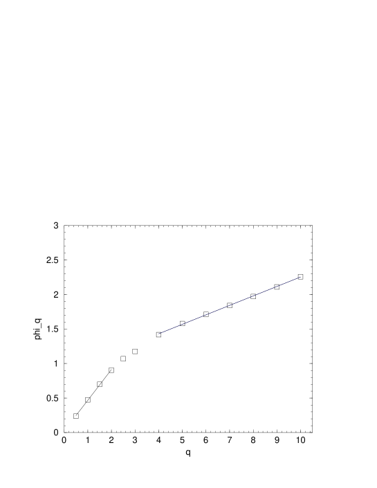
FIG. 7.: Exponent $\phi_{q}$ versus $q$. The slope of the two regions are 0.47 at $q<3$ and 0.14 at $q>3$.