Optimizing Epochal Evolutionary Search:
Population-Size Dependent Theory

Abstract

Epochal dynamics, in which long periods of stasis in an evolving population are punctuated by a sudden burst of change, is a common behavior in both natural and artificial evolutionary processes. We analyze the population dynamics for a class of fitness functions that exhibit epochal behavior using a mathematical framework developed recently. In the latter the approximations employed led to a population-size independent theory that allowed us to determine optimal mutation rates. Here we extend this approach to include the destabilization of epochs due to finite-population fluctuations and show that this dynamical behavior often occurs around the optimal parameter settings for efficient search. The resulting, more accurate theory predicts the total number of fitness function evaluations to reach the global optimum as a function of mutation rate, population size, and the parameters specifying the fitness function. We further identify a generalized error threshold, smoothly bounding the two-dimensional regime of mutation rates and population sizes for which evolutionary search operates efficiently.

Santa Fe Institute Working Paper 98-10-090

Contents

toc

I Designing Evolutionary Search

Evolutionary search algorithms are a class of stochastic optimization procedures inspired by biological evolution, e.g see Refs. [2, 18, 13, 20]: a population of candidate solutions evolves under selection and random “genetic” diversification operators. Evolutionary search algorithms have been successfully applied to a diverse variety of optimization problems; see, for example Refs. [3, 4, 5, 9, 11] and references therein. Unfortunately, and in spite of a fair amount of theoretical investigation, the mechanisms constraining and driving the dynamics of evolutionary search on a given problem are often not well understood.

There are very natural difficulties that are responsible for this situation. In mathematical terms evolutionary search algorithms are population-based discrete stochastic nonlinear dynamical systems. In general, the constituents of the search problem, such as the structure of the fitness function, selection, finite-population fluctuations, and genetic operators, interact in complicated ways to produce a rich variety of dynamical behaviors that cannot be easily understood in terms of the constituents individually. These complications make a strictly empirical approach to the question of whether and how to use evolutionary search problematic.

The wide range of behaviors exhibited by nonlinear population-based dynamical systems have been appreciated for decades in the field of mathematical population genetics. Unfortunately, this appreciation has not led to a quantitative predictive theory that is applicable to the problems of evolutionary search; something desired, if not required, for the engineering use of stochastic search methods.

We believe that a general, predictive theory of the dynamics of evolutionary search can be built incrementally, starting with a quantitative analytical understanding of specific problems and then generalizing to more complex situations. In this vein, the work presented here continues an attempt to unify and extend theoretical work in the areas of evolutionary search theory, molecular evolution theory, and mathematical population genetics. Our strategy is to focus on a simple class of problems that, nonetheless, exhibit some of the rich behaviors encountered in the dynamics of evolutionary search algorithms. Using analytical tools from statistical mechanics, dynamical systems theory, and the above mentioned fields we developed a detailed and quantitative understanding of the search dynamics for a class of problems that exhibit epochal evolution. On the one hand, this allows us to analytically predict optimal parameter settings for this class of problems. On the other hand, the detailed understanding of the behavior for this class of problems provides valuable insights into the emergent mechanisms that control the dynamics in more general settings of evolutionary search and in other population-based dynamical systems.

In a previous paper, Ref. [30], we showed how a detailed dynamical understanding, announced in Ref. [31] and expanded in Ref. [32], can be turned to practical advantage. Specifically, we determined how to set the mutation rate to reach, in the fewest number of fitness function evaluations, the global optimum in a wide class of fitness functions. Due to certain cancellations at the level of approximation used, the resulting theory lead to population-size independent predictions.

Here we extend this theory to include additional important effects, such as the increased search effort caused by the dynamical destabilization of epochs, to be explained below, which reintroduce the dependence on population size. The result is a more accurate theory that analytically predicts the total number of fitness function evaluations needed on average for the algorithm to discover the global optimum of the fitness function.

In addition, we develop a detailed understanding of the operating regime in parameter space for which the search is performed most efficiently. We believe this will provide useful guidance on how to set search algorithm parameters for more complex problems. In particular, our theory explains the marginally stable behavior of the dynamics when the parameters are set to minimize search effort. Most simply put, the optimal parameter setting occurs when the dynamics is as stochastic as possible without corrupting information stored in the population about the location of the current best genotypes. The results raise the general question of whether it is desirable for optimal search to run in dynamical regimes that are a balance of stability and instability. The mechanisms we identify suggest how this balance is, in fact, useful.

II Royal Staircase Fitness Functions

Choosing a class of fitness functions to analyze is a delicate compromise between generality, mathematical tractability, and the degree to which the class is representative of problems often encountered in evolutionary search. A detailed knowledge of the fitness function is very atypical of evolutionary search problems. If one knew the fitness function in detail, one would not have to run an evolutionary search algorithm to find high fitness solutions in the first place. The other extreme of assuming complete generality, however, cannot lead to enlightening results either, since averaged over all problems, all optimization algorithms perform equally well (or badly); see Ref. [34]. We thus focus on a specific subset of fitness functions, somewhere between these extremes, that we believe at least have ingredients typically encountered in evolutionary search problems and that exhibit widely observed dynamical behaviors in both natural and artificial evolutionary processes.

In our preceding paper, Ref. [30], we justified in some detail our particular choice of fitness function both in terms of biological motivations and in terms of optimization engineering issues. In short, many biological systems and optimization problems have highly degenerate genotype-to-phenotype maps; that is, the mapping from genetic specification to fitness is a many-to-one function. Consequently, the number of different fitness values that genotypes can take is much smaller than the number of different genotypes.

Additionally, due to the many-to-one mapping and since genotype spaces are generally of very high dimensionality, the genotype space tends to break into networks of “connected” sets of equal-fitness genotypes that can reach each other via elementary genetic variation steps such as point mutations. These connected subsets of isofitness genotypes are generally referred to as “neutral networks” in molecular evolution theory, see Refs. [10, 14, 15, 28, 33]. This leads us to posit that the genotype space for general search problems decomposes into a number of such neutral networks. We also assume that higher fitness networks are smaller in volume than low fitness networks. Finally, we assume that from any neutral network there exist connections to higher fitness networks such that, taken as a whole, the fitness landscape has no local optima other than the global optimum.

Under these assumptions, genotype space takes on a particular type of architecture: “subbasins” of the neutral networks are connected by “portals” leading between them and so to higher or lower fitness. Stated in the simplest terms possible, the evolutionary population dynamics then becomes a type of diffusion constrained by this architecture. For example, individuals in a population diffuse over neutral networks until a portal to a network of higher fitness is discovered and the population moves onto this network.

In order to model the behavior associated with the subbasin-portal architecture, we defined the class of Royal Staircase fitness functions that capture the essential elements sketched above. Importantly, this class of fitness functions is simple enough to admit a fairly detailed quantitative mathematical analysis of the associated epochal evolutionary dynamics.

The Royal Staircase fitness functions are defined as follows.

1. Genomes are specified by binary strings $s=s_{1}s_{2}\cdots s_{L},s_{i}\in\{0,1\},$ of length $L=NK$.

2. Reading the genome from left to right, the number $I(s)$ of consecutive $1$s is counted.

3. The fitness $f(s)$ of string $s$ with $I(s)$ consecutive ones, followed by a zero, is $f(s)=1+\lfloor I(s)/K\rfloor$. The fitness is thus an integer between $1$ and $N+1$.

Four observations are in order.

1. The fitness function has two parameters, the number $N$ of blocks and the number $K$ of bits per block. Fixing them determines a particular optimization problem or fitness “landscape”.

2. There is a single global optimum: the genome $s=1^{L}$—namely, the string of all $1$s—with fitness $f(s)=N+1$.

3. The proportion $\rho_{n}$ of genotype space filled by strings of fitness $n$ is given by:

   $$\rho_{n}=2^{-K(n-1)}\left(1-2^{-K}\right),$$ (1)

   for $n\leq N$. Thus, high fitness strings are exponentially more rare than low fitness strings.

4. For each block of $K$ bits, the all-$1$s pattern is the one that confers increased fitness on a string. Without loss of generality, any of the other $2^{K}-1$ configurations could have been chosen as the “correct” configuration, including different patterns for each of the $N$ blocks. Furthermore, since the GA here does not use crossover, arbitrary permutations of the $L$ bits in the fitness function definition leave the evolutionary dynamics unchanged.

The net result is that the Royal Staircase fitness functions implement the intuitive idea that increasing fitness is obtained by setting more and more bits in the genome “correctly”. One can only set correct bit values in sets of $K$ bits at a time, creating an “aligned” block, and in blocks from left to right. A genome’s fitness is proportional to the number of such aligned blocks. And since the $(n+1)$st block only confers fitness when all $n$ previous blocks are aligned as well, there is contingency between blocks. This realizes our view of the underlying architecture as a set of isofitness genomes that occur in nested neutral networks of smaller and smaller volume. (Cf. Figs. 1 and 2 of Ref. [30].)

III The Genetic Algorithm

For our analysis of evolutionary search we have chosen a simplified form of a genetic algorithm (GA) that does not include crossover and that uses fitness-proportionate selection. The GA is defined by the following steps.

1. Generate a population of $M$ bit strings of length $L=NK$ with uniform probability over the space of $L$-bit strings.

2. Evaluate the fitness of all strings in the population.

3. Stop, noting the generation number $t_{\rm opt}$, if a string with optimal fitness $N+1$ occurs in the population. Else, proceed.

4. Create a new population of $M$ strings by selecting, with replacement and in proportion to fitness, strings from the current population.

5. Mutate, i.e. change, each bit in each string of the new population with probability $q$.

6. Go to step 2.

When the algorithm terminates there have been $E=Mt_{\rm opt}$ fitness function evaluations.

In Ref. [30] we motivated our excluding crossover and discussed at some length the reasons that crossover’s role in epochal evolution is not expected to be significant due to population convergence effects.

This GA effectively has two parameters: the mutation rate $q$ and the population size $M$. A given optimization problem is specified by the fitness function in terms of $N$ and $K$. Stated most prosaically, then, the central goal of the following analysis is to find those settings of $M$ and $q$ that minimize the average number $\langle E\rangle$ of fitness function queries for given $N$ and $K$ required to discover the global optimum. Our approach is to develop analytical expressions for $E$ as a function of $N$, $K$, $M$, and $q$ and then to study the search-effort surface $E(q,M)$ at fixed $N$ and $K$. Before beginning the analysis, however, it is helpful to develop an appreciation of the basic dynamical phenomenology of evolutionary search on this class of fitness functions. Then we will be in a position to lay out the evolutionary equations of motion and analyze them.

IV Observed Population Dynamics

The typical behavior of a population evolving on a fitness “landscape” of connected neutral networks, such as defined above, alternates between long periods (epochs) of stasis in the population’s average fitness and sudden increases (innovations) in the average fitness. (See, for example, Fig. 1 of Ref. [32] and Fig. 1 of Ref. [30].)

We now briefly recount the experimentally observed behavior of typical Royal Staircase GA runs in which the parameters $q$ and $M$ are set close to their optimal setting. The reader is referred to Ref. [32] for a detailed discussion of the dynamical regimes this type of GA exhibits over a range of different parameter settings.

FIG. 1.: Examples of the Royal Staircase GA population dynamics with different parameter settings. The four plots show best fitness in the population (upper lines) and average fitness in the population (lower lines) as a function of time, measured in generations. The fitness function and GA parameters are given in each plot. In each case we have chosen $q$ and $M$ in the neighborhood of their optimal settings (see later) for each of the four values of $N$ and $K$.

Figure 1 illustrates the GA’s behavior at four different parameter settings. Each individual figure plots the best fitness in the population (upper lines) and the average fitness $\langle f\rangle$ in the population (lower lines) as a function of the number of generations. Each plot is produced from a single GA run. In all of these runs the average fitness $\langle f\rangle$ in the population goes through stepwise changes early in the run, alternating epochs of stasis with sudden innovations in fitness. Later in each run, especially for those in Figs. 1(b) and 1(d), $\langle f\rangle$ tends to have higher fluctuations and the epochal nature of the dynamics becomes unclear.

In the GA runs the population starts out with strings that only have relatively low fitness, say fitness $n$ (in all four plots of Fig. 1 we have $n=1$). Selection and mutation then establish an equilibrium in the population until a string aligns the $n$th block, and descendants of this string with fitness $n+1$ spread through the population. A new equilibrium is then established until a string of fitness $n+2$ is discovered and so on, until finally, a string of fitness $N+1$ is discovered.

Notice that $\langle f\rangle$ roughly tracks the epochal behavior of the best fitness in the population. Every time a newly discovered higher fitness string has spread through the population, $\langle f\rangle$ reaches a new, higher equilibrium value around which it fluctuates. As a run progresses to higher epochs, $\langle f\rangle$ tends to have higher fluctuations and the epochal nature of the dynamics is obscured. This is a result of the fact that for the highest epochs the difference between $\langle f\rangle$ in consecutive epochs is smaller than the average fitness fluctuations induced by the finite-population sampling; see Ref. [32].

Notice, too, that often the best fitness shows a series of brief jumps to higher fitness during an epoch. When this occurs strings of higher fitness are discovered but, rather than spreading through the population, are lost within a few generations.

For each of the four settings of $N$ and $K$ we have chosen the values of $q$ and $M$ such that the average total number $\langle E\rangle$ of fitness function evaluations to reach the global optimum for the first time is minimal. Thus, the four plots illustrate the GA’s typical dynamics close to optimal $(q,M)$-parameter settings.

Despite what appears at first blush to be relatively small variations in fitness function and GA parameters, there is a large range, almost a factor of $10$, in times to reach the global optimum across the runs. Thus, there can be a strong parameter dependence in search times. It also turns out that the standard deviation $\sigma$ of the mean total number $\langle E\rangle$ of fitness function evaluations is of the same order as $\langle E\rangle$. (See Table I.) Thus, there are large run-to-run variations in the time to reach the global optimum. This is true for all parameter settings with which we experimented, of which only a few are reported here.

Having addressed the commonalities between runs, we now turn to additional features that each illustrates. Figure 1(a) shows the results of a GA run with $N=8$ blocks of $K=8$ bits each, a mutation rate of $q=0.005$, and a population size of $M=200$. During the epochs, the best fitness in the population hops up and down several times before it finally jumps up and the new more-fit strings stabilize in the population. This transition is reflected in the average fitness also starting to move upward. In this particular run, it took the GA approximately $3.4\times 10^{5}$ fitness function evaluations (1700 generations) to discover the global optimum for the first time. Over 500 runs, the GA takes on average $5.3\times 10^{5}$ fitness function evaluations to reach the global optimum for these parameters. The inherent large per-run variation means in this case that some runs take less than $10^{5}$ function evaluations and that others take many more than $10^{6}$.

Figure 1(b) plots a run with $N=6$ blocks of length $K=6$ bits, a mutation rate of $q=0.016$, and a population size of $M=150$. The GA discovered the global optimum after approximately $4.8\times 10^{4}$ fitness function evaluations (325 generations). For these parameters, the GA uses approximately $5.5\times 10^{4}$ fitness function evaluations on average to reach the global fitness optimum. Notice that the global optimum is only consistently present in the population between generations $530$ generation $570$. After that, the global optimum is lost again until after generation $800$. As we will show, this is a typical feature of the GA’s behavior for parameter settings close to those that give minimal $\langle E\rangle$. The global fitness optimum often only occurs in relatively short bursts after which it is lost again from the population. Notice also that there is only a small difference in $\langle f\rangle$ depending whether the best fitness is either $6$ or $7$ (the optimum).

Figure 1(c) shows a run for a small number ($N=4$) of large ($K=10$) blocks. The mutation rate is $q=0.014$ and the population size is again $M=150$. As in the three other runs we see that $\langle f\rangle$ goes through epochs punctuated by rapid increases in $\langle f\rangle$. We also see that the best fitness in the population jumps several times before the population fixes on a higher fitness string. The GA takes about $1.9\times 10^{5}$ fitness function evaluations on average to discover the global optimum for these parameter settings. In this run, the GA first discovered the global optimum after $2.7\times 10^{5}$ fitness function evaluations. Notice that the optimum never stabilized in the population.

Finally, Fig. 1(d) shows a run with a large number ($N=10$) of small ($K=5$) blocks. The mutation rate is $q=0.008$ and the population size is $M=100$. Notice that in this run, the best fitness in the population alternates several times between fitnesses $8$, $9$, and $10$ before it reaches (fleetingly) the global fitness optimum of $11$. Quickly after it has discovered the global optimum, it disappears again and the best fitness in the population largely alternates between $9$ and $10$ from then on. It is notable that this intermittent behavior of the best fitness is barely discernible in the behavior of $\langle f\rangle$. It appears to be lost in the “noise” of the average fitness fluctuations. The GA takes about $1.2\times 10^{5}$ fitness function evaluations on average at these parameter settings to reach the global optimum; while in this particular run the GA took $1.6\times 10^{5}$ fitness function evaluations (1640 generations) to briefly reach the optimum for the first time.

V Statistical Dynamics of Evolutionary Search

In Refs. [31] and [32] we developed the statistical dynamics of genetic algorithms to analyze the behavioral regimes of a GA searching the Royal Road fitness functions, which are closely related to the Royal Staircase fitness functions just defined. The analysis here builds on those results and, additionally, is a direct extension of the optimization analysis and calculations in Ref. [30]. We briefly review the essential points from these previous papers. We refer the reader to Ref. [32] for a detailed description of the similarities and differences of our theoretical approach with other theoretical approaches such as the work by Prug̈el-Bennett, Rattray, and Shapiro, Refs. [25, 26, 27], the diffusion equation methods developed by Kimura, Refs. [16, 17], and the quasispecies theory, Ref. [7].

$N$	$K$	$M$	$q$	$\langle E\rangle$	$\sigma$
8	8	200	$0.005$	$5.3\times 10^{5}$	$2.1\times 10^{5}$
6	6	150	$0.016$	$5.5\times 10^{4}$	$3.0\times 10^{4}$
4	10	150	$0.014$	$1.9\times 10^{5}$	$1.0\times 10^{5}$
10	5	100	$0.008$	$1.2\times 10^{5}$	$4.9\times 10^{4}$

TABLE I.: Mean $\langle E\rangle$ and standard deviations $\sigma$ of the expected number of fitness function evaluations for the Royal Staircase fitness functions and GA parameters shown in the runs of Fig. 1. The estimates were made from 500 GA runs.

A Macrostate Space

Formally, the state of a population in an evolutionary search algorithm is only specified when the frequency of occurrence of each of the $2^{L}$ genotypes is given. Thus, the dimension of the corresponding microscopic state space is very large. One immediate consequence is that the evolutionary dynamic, on this level, is given by a stochastic (Markovian) operator of size ${\cal O}(2^{L}\times 2^{L})$. Generally, using such a microscopic description makes analytical and quantitative predictions of the GA’s behavior unwieldy. Moreover, since the practitioner is generally interested in the dynamics of some more macroscopic statistics, such as best and average fitness, a microscopic description is uninformative unless an appropriate projection onto the desired macroscopic statistic is found.

With these difficulties in mind, we choose to describe the macroscopic state of the population by its fitness distribution, denoted by a vector $\vec{P}=(P_{1},P_{2},\ldots,P_{N+1})$, where the components $0\leq P_{f}\leq 1$ are the proportions of individuals in the population with fitness $f=1,2,\ldots,N+1$. We refer to $\vec{P}$ as the phenotypic quasispecies, following its analog in molecular evolution theory; see Refs. [6, 7, 8]. Since $\vec{P}$ is a distribution, it is normalized:

$$\sum_{f=1}^{N+1}P_{f}=1.$$ (2)

The average fitness $\langle f\rangle$ of the population is given by:

$$\langle f\rangle=\sum_{f=1}^{N+1}fP_{f}.$$ (3)

B The Evolutionary Dynamic

The fitness distribution $\vec{P}$ does not uniquely specify the microscopic state of the population; that is, there are many microstates with the same fitness distribution. An essential ingredient of the statistical dynamics approach is to assume a maximum entropy distribution of microstates conditioned on the macroscopic fitness distribution. Note that our approach shares a focus on fitness distributions and maximum entropy methods with that of Prug̈el-Bennett, Rattray, and Shapiro, Refs. [25, 26, 27]. In our case, the maximum entropy assumption entails that, given a fitness distribution $\vec{P}(t)$ at generation $t$, each microscopic population state with this fitness distribution is equally likely to occur. Given this assumption, we can construct a generation operator ${\bf G}$ that acts on the current fitness distribution to give the expected fitness distribution of the population at the next time step. (See $\vec{P}(t)\rightarrow{\bf G}[\vec{P}(t)]$ illustrated in Fig. 2.) In the limit of infinite populations, which is similar to the thermodynamic limit in statistical mechanics, this operator ${\bf G}$ maps the current fitness distribution $\vec{P}(t)$ deterministically to the fitness distribution $\vec{P}(t+1)$ at the next time step; that is,

$$\vec{P}(t+1)={\bf G}[\vec{P}(t)]~{}.$$ (4)

Simulations indicate that for very large populations ($M\gtrapprox 2^{L}$) the dynamics on the level of fitness distributions is indeed deterministic and given by the above equation; thereby justifying the maximum entropy assumption in this limit.

The operator ${\bf G}$ consists of a selection operator ${\bf S}$ and a mutation operator ${\bf M}$:

$${\bf G}={\bf M}\cdot{\bf S}.$$ (5)

The selection operator encodes the fitness-level effect of selection on the population; and the mutation operator, the fitness-level effect of mutation. Appendixes A and B review the construction of these operators for our GA and the Royal Staircase fitness functions.

For now, we note that the infinite population dynamics can be obtained by iteratively applying the operator ${\bf G}$ to the initial fitness distribution $\vec{P}(0)$. Thus, the solutions to the macroscopic equations of motion, in the limit of infinite populations, are formally given by

$$\vec{P}(t)={\bf G}^{(t)}[\vec{P}(0)]~{}.$$ (6)

Recalling Eq. (1), it is easy to see that the initial fitness distribution $\vec{P}(0)$ is given by:

$$P_{n}(0)=2^{-K(n-1)}\left(1-2^{-K}\right)\;,~{}1\leq n\leq N~{},$$ (7)

and

$$P_{N+1}(0)=2^{-KN}.$$ (8)

As shown in Refs. [31] and [32], despite ${\bf G}$’s nonlinearity, it can be linearized such that the $t$th iterate ${\bf G}^{(t)}$ can be directly obtained by solving for the eigenvalues and eigenvectors of the linearized version ${\bf\tilde{G}}$. This leads to a closed-form solution of the infinite-population dynamics specified by Eq. (6).

C Finite Population Sampling

For large ($M\gtrapprox 2^{L}$) and infinite populations the dynamics of the fitness distribution is qualitatively very different from the behavior shown in Fig. 1: $\langle f\rangle$ increases smoothly and monotonically to an asymptote over a small number of generations. That is, there are no epochs. The reason is that for an infinite population, all genotypes are present in the initial population. Instead of the evolutionary dynamics discovering fitter strings over time, it essentially only expands the proportion of globally optimal strings already present in the initial population at $t=0$. In spite of the qualitatively different dynamics for large populations, we showed in Ref. [32] that the (infinite population) operator ${\bf G}$ is the essential ingredient for describing the finite-population dynamics with its epochal dynamics as well.

There are two important differences between the infinite-population dynamics and that with finite populations. The first is that with finite populations the components $P_{n}$ cannot take on continuous values between $0$ and $1$. Since the number of individuals with fitness $n$ in the population is necessarily an integer, the values of $P_{n}$ are quantized in multiples of $1/M$. Thus, the space of allowed finite population fitness distributions turns into a regular lattice in $N+1$ dimensions with a lattice spacing of $1/M$ within the simplex specified by normalization (Eq. (2)).

Second, due to the sampling of members in the finite population, the dynamics of the fitness distribution is no longer deterministic. In general, we can only determine the conditional probabilities ${\rm Pr}[\vec{Q}|\vec{P}]$ that a given fitness distribution $\vec{P}$ leads to another $\vec{Q}=(Q_{1},\ldots,Q_{N+1})$ in the next generation.

FIG. 2.: Illustration of the stochastic dynamics involved in going from one generation to the next starting with finite population $\vec{P}$, moving to the next (expected) population ${\bf G}[\vec{P}]$, and then sampling to obtain the distribution ${\rm Pr}[\vec{Q}|\vec{P}]$ of finite populations at the next time. The width of the latter distribution is inversely proportional to the population size $M$. Note that the underlying state space is a discrete lattice with spacing $1/M$.

It turns out that the probabilities ${\rm Pr}[\vec{Q}|\vec{P}]$ are given by a multinomial distribution with mean ${\bf G}[\vec{P}]$:

$${\rm Pr}[\vec{Q}|\vec{P}]=M!\prod_{n=1}^{N+1}\frac{\left({\bf G}_{n}[\vec{P}]\right)^{m_{n}}}{m_{n}!}~{}.$$ (9)

where $Q_{n}=m_{n}/M$, with $0\leq m_{n}\leq M$ integers. (The stochastic effects of finite sampling are illustrated in Fig. 2.) For any finite-population fitness distribution $\vec{P}$ the (infinite population) operator ${\bf G}$ gives the GA’s average dynamics over one time step, since by Eq. (9) the expected fitness distribution at the next time step is ${\bf G}[\vec{P}]$. Note that the components ${\bf G}_{n}[\vec{P}]$ need not be multiples of $1/M$. Therefore, the actual fitness distribution $\vec{Q}$ at the next time step is not ${\bf G}[\vec{P}]$, but is instead one of the allowed lattice points in the finite-population state space. Since the variance around the expected distribution ${\bf G}[\vec{P}]$ is proportional to $1/M$, $\vec{Q}$ tends to be one of the lattice points close to ${\bf G}[\vec{P}]$.

D Epochal Dynamics

For finite populations, the expected change $\langle d\vec{P}\rangle$ in the fitness distribution over one generation is given by:

$$\langle d\vec{P}\rangle={\bf G}[\vec{P}]-\vec{P}.$$ (10)

Assuming that some component $\langle dP_{i}\rangle$ is much smaller than $1/M$, the actual change in component $P_{i}$ is likely to be $dP_{i}=0$ for a long succession of generations. That is, if the size of the “flow” $\langle dP_{i}\rangle$ in some direction $i$ is much smaller than the lattice spacing ($1/M$) for the finite population, we expect the fitness distribution to not change in direction (fitness) $i$.

In Refs. [31] and [32] we showed this is the mechanism by which finite populations cause epochal dynamics. For the Royal Staircase fitness functions, we have that whenever fitness $n$ is the highest in the population, such that $P_{i}=0$ for all $i>n$, the rate at which higher fitness strings are discovered is very small: $\langle dP_{i}\rangle\ll 1/M$ for all $i>n$ and population size $M$ not too large. A period of stasis (an evolutionary epoch) thus corresponds to the time the population spends before it discovers a higher fitness string. More formally, each epoch $n$ corresponds to the population being restricted to a region in the $n$-dimensional lower-fitness subspace consisting of fitnesses $1$ to $n$ of the macroscopic state space. Stasis occurs because the flow out of this subspace is much smaller than the finite-population induced lattice spacing.

As the experimental runs of Fig. 1 illustrated, each epoch in the average fitness is associated with a (typically) constant value of the best fitness in the population. More detailed experiments reveal that not only is $\langle f\rangle$ constant on average during the epochs, in fact the entire fitness distribution $\vec{P}$ fluctuates in an approximately Gaussian way around some constant fitness distribution $\vec{P}^{n}$ during the epoch $n$—the generations when $n$ is the highest fitness in the population.

As was shown in Ref. [32], each epoch fitness distribution $\vec{P}^{n}$ is the unique fixed point of the operator ${\bf G}$ restricted to the $n$-dimensional subspace of strings with $1\leq f\leq n$. That is, if ${\bf G}^{n}$ is the projection of the operator ${\bf G}$ onto the $n$-dimensional subspace of fitnesses from $1$ up to $n$, then we have:

$${\bf G}^{n}[\vec{P}^{n}]=\vec{P}^{n}~{}.$$ (11)

By Eq. (3), then, the average fitness $f_{n}$ in epoch $n$ is given by:

$$f_{n}=\sum_{j=1}^{n}jP^{n}_{j}.$$ (12)

Thus, the fitness distributions $\vec{P}^{n}$ during epoch $n$ are obtained by finding the fixed point of ${\bf G}$ restricted to the first $n$ dimensions of the fitness distribution space. We will pursue this further in the next section.

To summarize at this point, the statistical dynamics analysis is tantamount to the following qualitative picture. The global dynamics can be viewed as an incremental discovery of successively more (macroscopic) dimensions of the fitness distribution space. Initially, only strings of low fitness are present in the initial population. The population stabilizes on the epoch fitness distribution $\vec{P}^{n}$ corresponding to the best fitness $n$ in the initial population. The fitness distribution fluctuates around the $n$-dimensional vector $\vec{P}^{n}$ until a string of fitness $n+1$ is discovered and spreads through the population. The population then settles into $(n+1)$-dimensional fitness distribution $\vec{P}^{n+1}$ until a string of fitness $n+2$ is discovered, and so on, until the global optimum at fitness $N+1$ is found. In this way, the global dynamics can be seen as stochastically hopping between the different epoch distributions $\vec{P}^{n}$, unfolding a new macroscopic dimension of the fitness distribution space each time a higher fitness string is discovered.

Whenever mutation creates a string of fitness $n+1$, this string may either disappear before it spreads, seen as the transient jumps in best fitness in Fig. 1, or it may spread, leading the population to fitness distribution $\vec{P}^{n+1}$. We call the latter process an innovation. Through an innovation, a new (macroscopic) dimension of fitness distribution space becomes stable. Fig. 1 also showed that it is possible for the population to fall from epoch $n$ (say) down to epoch $n-1$. This happens when, due to fluctuations, all individuals of fitness $n$ are lost from the population. We refer to this as a destabilization of epoch $n$. Through a destabilization, a dimension can, so to speak, collapse. For some parameter settings, such as shown in Figs. 1(a) and 1(c), this is very rare. In these cases, the time for the GA to reach the global optimum is mainly determined by the time it takes to discover strings of fitness $n+1$ in each epoch $n$. For other parameter settings, however, such as in Figs. 1(b) and 1(d), the destabilizations play an important role in how the GA reaches the global optimum. In these regimes, destabilization must be taken into account in calculating search times. This is especially important in the current setting since, as we will show, the optimized GA often operates in this type of marginally stable parameter regime.

VI Quasispecies Distributions and Epoch Fitness Levels

During epoch $n$ the quasispecies fitness distribution $\vec{P}^{n}$ is given by a fixed point of the operator ${\bf G}^{n}$. To obtain this fixed point we linearize the generation operator by taking out the factor $\langle f\rangle$, thereby defining a new operator ${\bf\tilde{G}}^{n}$ via:

$${\bf G}^{n}=\frac{1}{\langle f\rangle}{\bf\tilde{G}}^{n},$$ (13)

where $\langle f\rangle$ is the average fitness of the fitness distribution that ${\bf G}^{n}$ acts upon; see App. A. The operator ${\bf\tilde{G}}^{n}$ is just an ordinary (linear) matrix operator and the quasispecies fitness distribution $\vec{P}^{n}$ is nothing other than the principal eigenvector of this matrix (normalized in probability). Conveniently, one can show that the principal eigenvalue $f_{n}$ of ${\bf\tilde{G}}^{n}$ is also the average fitness of the quasispecies distribution. In this way, obtaining the quasispecies distribution $\vec{P}^{n}$ reduces to calculating the principal eigenvector of the matrix ${\bf\tilde{G}}^{n}$. Again, the reader is referred to Ref. [32].

The matrices ${\bf\tilde{G}}^{n}$ are generally of modest size: i.e., their dimension is smaller than the number of blocks $N$ and substantially smaller than the dimension of genotype space. Due to this we can easily obtain numerical solutions for the epoch fitnesses $f_{n}$ and the epoch quasispecies distributions $\vec{P}^{n}$. For a clearer understanding of the functional dependence of the epoch fitness distributions on the GA’s parameters, however, App. C recounts analytical approximations to the epoch fitness levels $f_{n}$ and quasispecies distributions $\vec{P}^{n}$ developed in Ref. [30].

The result is that the average fitness $f_{n}$ in epoch $n$, which is given by the largest eigenvalue, is equal to the largest diagonal component of the analytical approximation to ${\bf\tilde{G}}^{n}$ derived in App. C. That is,

$$f_{n}=n(1-q)^{(n-1)K}~{}.$$ (14)

The epoch quasispecies is given by:

$$P^{n}_{i}=\frac{(1-\lambda)n\lambda^{n-1-i}}{n\lambda^{n-1-i}-i}\prod_{j=1}^{i-1}\frac{n\lambda^{n-j}-j}{n\lambda^{n-1-j}-j}~{},$$ (15)

where $\lambda=(1-q)^{K}$ is the probability that a block will undergo no mutations. For the following, we are actually interested in the most-fit quasispecies component $P^{n}_{n}$ in epoch $n$. For this component, Eq. (15) reduces to

$$P^{n}_{n}=\lambda^{n-1}\prod_{j=1}^{n-1}\frac{f_{n}-f_{j}}{f_{n}-\lambda f_{j}}~{},$$ (16)

where we have expressed the result in terms of of the epoch fitness levels $f_{j}$.

VII Mutation Rate Optimization

In the previous sections we argued that the GA’s behavior can be viewed as (occasionally) stochastically hopping from epoch to epoch—when the search discovers a string with increased fitness that spreads in the population. Assuming the total time to reach this global optimum is dominated by the time the GA spends in the epochs, Ref. [30] developed a way to tune the mutation rate $q$ such that the time the GA spends in an epoch is minimized. We briefly review this here before moving on to the more general theory that includes population-size effects and epoch destabilization.

Optimizing the mutation rate amounts to finding a balance between two opposing effects of varying mutation rate. On the one hand, when the mutation rate is increased, the average number of mutations in the unaligned blocks goes up thereby increasing the probability of creating a new aligned block. On the other hand, due to the increased number of deleterious mutations, the equilibrium proportions $P^{n}_{n}$ of individuals in the highest fitness class during each epoch $n$ decreases.

In Ref. [30] we derived an expression for the probability $C_{n+1}$ to create, over one generation in epoch $n$, a string of fitness $n+1$ that will stabilize by spreading through the population. This is given by

$$C_{n+1}=MP^{n}_{n}P_{a}\pi_{n}(\lambda)~{},$$ (17)

where $P_{a}=(1-\lambda)/(2^{K}-1)$ is the probability of aligning a block (App. B) and $\pi_{n}(\lambda)$ is the probability that a string of fitness $n+1$ will spread, as opposed to being lost through a fluctuation or a deleterious mutation. This latter probability largely depends on the relative average fitness difference of epoch $n+1$ over epoch $n$. Denoting this difference as

$$\gamma_{n}=\frac{f_{n+1}-f_{n}}{f_{n}}=\left(1+\frac{1}{n}\right)\lambda-1,$$ (18)

and using a diffusion equation approximation (see Ref. [32]), we found:

$$\pi_{n}(\lambda)=\frac{1-\left(1-\frac{1}{M}\right)^{2M\gamma_{n}+1}}{1-\left(1-P^{n+1}_{n+1}\right)^{2M\gamma_{n}+1}}.$$ (19)

If $P^{n+1}_{n+1}\gg 1/M$, this reduces to a population-size independent estimate of the spreading probability

$$\pi_{n}\approx 1-e^{-2\gamma_{n}}.$$ (20)

If one allows for changing the mutation rate between epochs, one would minimize the time spent in each epoch by maximizing $C_{n+1}$. Note that $C_{n+1}$ depends on $q$ only through $\lambda$. The optimal mutation rate in each epoch $n$ is determined by estimating the optimal value $\lambda_{o}$ of $\lambda$ for each $n$. Although the optimal $\lambda_{o}$ can be determined as the solution of an algebraic equation, we found in Ref. [30] that it is well approximated by

$$\lambda_{o}(n)\approx 1-\frac{1}{3n^{1.175}}~{}.$$ (21)

For large $n$ this gave the optimal mutation rate as

$$q_{o}\approx\frac{1}{3Kn^{1.175}}~{},n\gg 1~{}.$$ (22)

Thus, the optimal mutation rate drops as a power-law in both $n$ and $K$. This implies that if one is allowed to adapt the mutation rate during the run, the mutation rate should decrease as a GA run progresses so that the search will find the global optimum as quickly as possible. We pursue this idea more precisely elsewhere by considering an adaptive mutation rate scheme for a GA.

We now turn to the simpler problem of optimizing mutation rate for the case of a constant mutation rate throughout a GA run. In Ref. [30] we used Eq. (17) to estimate the total number $E$ of fitness function evaluations the GA uses on average before an optimal string of fitness $N+1$ is found. As a first approximation, we assumed that the GA visits all epochs, that the time spent in innovations between them is negligible, and that epochs are always stable. By epoch stability we that mean it is highly unlikely that strings with the current highest fitness will disappear from the population through a fluctuation, once such strings have spread. These assumptions appear to hold for the parameters of Figs. 1(a) and 1(c). They may hold even for the parameters of Fig. 1(b), but they most likely do not for Fig. 1(d). For the parameters of Fig. 1(d), we see that the later epochs ($n=9$, and $10$) easily destabilize a number of times before the global optimum is found. Although we will develop a generalization that addresses this more complicated behavior in the next sections, it is useful to work through the optimization of mutation rate first.

The average number $T_{n}$ of generations that the population spends in epoch $n$ is simply $1/C_{n+1}$, the inverse of the probability that a string of fitness $n+1$ will be discovered and spread through the population. For a population of size $M$, the number of fitness function evaluations per generation is $M$, so that the total number $E_{n}$ of fitness function evaluations in epoch $n$ is given by $MT_{n}$. More explicitly, we have:

$$E_{n}=\left(P^{n}_{n}P_{a}\pi_{n}\right)^{-1}.$$ (23)

That is, the total number of fitness function evaluations in each epoch is independent of the population size $M$. This is due to two facts, given our approximations. First, the epoch lengths, measured in generations, are inversely proportional to $M$, while the number of fitness function evaluations per generation is $M$. Second, since for stable epochs $P^{n}_{n}\gg 1/M$, the probability $\pi_{n}$ is also independent of population size $M$; recall Eq. (20).

The total number of fitness function evaluations $E(\lambda)$ to reach the global optimum is simply given by substituting into Eq. (23) our analytical expressions for $P^{n}_{n}$ and $\pi_{n}$, Eqs. (16) and (20), and then summing $E_{n}(\lambda)$ over all epochs $n$ from $1$ to $N$. We found that:

$$E(\lambda)=\sum_{n=1}^{N}\frac{1}{P_{a}\pi_{n}(\lambda)}\prod_{i=1}^{n-1}\frac{n\lambda^{n-i-1}-i}{n\lambda^{n-i}-i}~{}.$$ (24)

Note that in the above equation $\pi_{N}=1$ by definition because the algorithm terminates as soon as a string of fitness $N+1$ is found. That is, strings of fitness $N+1$ need not spread through the population. The optimal mutation rate for an entire run is obtained by minimizing Eq. (24) with respect to $\lambda$.

FIG. 3.: Average total number $\langle E\rangle$ of fitness function evaluations as a function of mutation rate $q$, from the theory (dashed), Eq. (24), and from experimental estimates (solid). The fitness function parameter settings are $N=4$ blocks of length $K=10$ bits. The mutation rate runs from $q=0.001$ to $q=0.028$. Experimental data points are estimates over $250$ runs. The experimental curves show four different population sizes; $M=80$, $M=140$, $M=230$, and $M=380$.

Figure 3 shows for $N=4$ blocks of length $K=10$ bits the dependence of the average total number $E(q)$ of fitness function evaluations on the mutation rate $q$. The dashed line is the theoretical prediction of Eq. (24); while the solid lines show the experimentally estimated values of $\langle E\rangle$ for four different population sizes. Each experimental data point is an estimate obtained from $250$ GA runs. Figure 3 illustrates in a compact form the findings of Ref. [30], which can be summarized as follows.

1. At fixed population size $M$, there is a smooth cost function $E(q)$ as a function of mutation rate $q$. It has a single and shallow minimum $q_{o}$, which is accurately predicted by the theory.

2. The curve $E(q)$ is everywhere concave.

3. The theory slightly underestimates the experimentally obtained $\langle E\rangle$.

4. The optimal mutation rate $q_{o}$ roughly occurs in the regime where the highest epochs are marginally stable; see Fig. 1.

5. For mutation rates lower than $q_{o}$ the experimentally estimated total number of fitness function evaluations $\langle E\rangle$ grows steadily and becomes almost independent of the population size $M$. (This is where the experimental curves in Fig. 3 overlap.) For mutation rates larger than $q_{o}$ the total number of fitness function evaluations does depend on $M$, which is not explained by the theory of Ref. [30].

6. There is mutational error threshold in $q$ that bounds the upper limit in $q$ of the GA’s efficient search regime. Above the threshold, which is population-size independent, suboptimal strings of fitness $N$ cannot stabilize in the population, even for very large population sizes. This error threshold is also correctly predicted by the theory. It occurs around $q_{c}=0.028$ for $N=4$ and $K=10$.

VIII Epoch Destabilization: Population-Size Dependence

We now extend the above analysis to account for $E$’s dependence on population size. This not only improves the parameter-optimization theory, but also leads us to consider a number of issues and mechanisms that shed additional light on how GAs work near their optimal parameter settings. Since it appears that optimal parameter settings often lead the GA to run in a behavioral regime were the population dynamics is marginally stable in the higher epochs, we consider how destabilization dynamics affects the time to discover the global optimum.

We saw in Figs. 1(b) and 1(d) that, around the optimal parameter settings, the best fitness in the population can show intermittent behavior. Apparently, fluctuations sometimes cause an epoch’s current best strings (of fitness $n$) in the population to disappear. The best fitness then drops to $n-1$. Often, strings of fitness $n$ are rediscovered later on. Qualitatively, what happens during these destabilizations is that, since the proportion $P^{n}_{n}$ of individuals in the highest fitness class decreases for increasing $n$ and $q$ (Eq. (16)), for small population sizes the absolute number of individuals in the highest fitness class approaches a single string; i.e., $MP^{n}_{n}\approx 1$ in higher epochs. When this happens, it is likely that all individuals of fitness $n$ are lost through a deleterious fluctuation and the population falls back onto epoch $n-1$. Somewhat more precisely, whenever the standard deviation of fluctuations in the proportion $P_{n}$ of individuals with fitness $n$ becomes as small as their equilibrium proportion $P^{n}_{n}$, destabilizations start to become a common occurrence.

Since the probability of a destabilization is sensitive to the population size $M$, this dynamical effect introduces population-size dependence in the average total number $\langle E\rangle$ of fitness function evaluations.

As we just noted, the theory for $E(q)$ used in Ref. [30] assumed that all epochs are stable, leading to a population-size independent theory. However, as is clear from Fig. 1(d), one should take into account the (population-size dependent) probability of epoch $n$ destabilizing several times to epoch $n-1$ before the population moves to epoch $n+1$. For example, if during epoch $n$ the population is $3$ times as likely to destabilize to epoch $n-1$ compared to innovating to epoch $n+1$, then we expect epoch $n$ to disappear three times before moving to epoch $n+1$. Assuming that epoch $n-1$ is stable, this increases the number of generations spent in epoch $n$ by roughly three times the average number of generations spent in epoch $n-1$.

To make these ideas precise we introduce a Markov chain model to describe the “hopping” up and down between the epochs. The Markov chain has $N+1$ states, each representing an epoch. In every generation there are probabilities $p^{+}_{n}$ to innovate from epoch $n$ to epoch $n+1$ and $p^{-}_{n}$ to destabilize, falling from epoch $n$ to epoch $n-1$. The globally optimum state $N+1$ is an absorbing state. Starting from epoch $1$ we calculate the expected number $T$ of generations for the population to reach the absorbing state for the first time.

The innovation probabilities $p^{+}_{n}$ are just given by the $C_{n+1}$ of Eq. (17):

$$p^{+}_{n}=C_{n+1}=\frac{M}{E_{n}},$$ (25)

where $E_{n}$ is given by the approximation of Eq. (23). Note that when $MP^{n}_{n}$ approaches $1$ the spreading probability $\pi_{n}$, as given by Eq. (19), becomes population-size dependent as well, and we use Eq. (19) rather than Eq. (20). To obtain the destabilization probabilities $p^{-}_{n}$ we assume that in each generation the population has an equal and independent probability to destabilize to epoch $n-1$. This probability is given by the inverse of the average time until a destabilization occurs.

In Ref. [32] we studied the destabilization mechanism using a diffusion equation method. We derived an analytical approximation for the average number of generations $D_{n}$ until epoch $n$ destabilizes and falls back onto epoch $n-1$. The result is:

$$D_{n} = \frac{MP^{n}_{n}}{1-P^{n}_{n}}$$ (26)

$$+ \frac{\pi}{2\mu_{n}}{\rm erfi}\left[\sqrt{\frac{M\mu_{n}P^{n}_{n}}{1-P^{n}_{n}}}\right]{\rm erf}\left[\sqrt{\frac{M\mu_{n}(1-P^{n}_{n})}{P^{n}_{n}}}\right],$$ (27)

where ${\rm erf}(x)$ is the error function and ${\rm erfi}(x)={\rm erf}(ix)/i$ is the imaginary error function.

In Ref. [32] we pointed out the connection between the above formula and error thresholds in the theory of molecular evolution. Generally, error thresholds denote the boundary in parameter space between a regime where a certain high fitness string, or an equivalence class of high fitness strings, is stable in the population, and a regime where it is unstable. In the case of a single high fitness “master sequence” one speaks of a genotypic error threshold; see Refs. [1, 7, 22, 29]. In the case of an equivalence class of high fitness strings, one speaks of a phenotypic error threshold; see Refs. [14, 28].

A sharply defined error threshold generally only occurs in the limit of infinite populations and infinite string length [19], but extensions to finite population cases have been studied in Refs. [1, 22, 28]. In Ref. [28], for example, the occurrence of a finite-population phenotypic error threshold was defined by the equality of the standard deviation and the mean of the number of individuals of the highest fitness class. This definition is in accord with Eq. (27): the argument of ${\rm erfi(x)}$, $\sqrt{M\mu_{n}P^{n}_{n}/(1-P^{n}_{n})}$, is exactly the ratio between the mean proportion $P^{n}_{n}$ and standard deviation of the number of individuals with fitness $n$, as derived in Ref. [32]. The function ${\rm erfi}(x)$ is a very rapidly growing function of its argument: ${\rm erfi}(x)\approx\exp(x^{2})/x$ for $x$ larger than $1$. Therefore, $\sqrt{M\mu_{n}P^{n}_{n}/(1-P^{n}_{n})}$ being either smaller (larger) than $1$ is a reasonable criterion for the instability (stability) of an epoch. Of course, this is simply a way of summarizing the more detailed information contained in Eq. (27).

The constant $\mu_{n}$ in Eq. (27) is the average decay rate of fluctuations in the number of individuals in the highest fitness class around its equilibrium value $P^{n}_{n}$. The value of $\mu_{n}$ for epoch $n$ can be calculated in terms of the relative sizes of the fluctuations in the directions of all lower-lying epochs. This calculation was performed explicitly in Ref. [32]. Formally, one needs to rotate the covariance matrix of sampling fluctuations during epoch $n$ to the basis of epoch eigenvectors $\vec{P}^{i}$. The covariance matrix of sampling fluctuations during epoch $n$ is approximately given by:

$$\langle dP_{i}dP_{j}\rangle=\frac{P^{n}_{i}(\delta_{ij}-P^{n}_{j})}{M}.$$ (28)

Defining the matrix ${\bf R}$ such that its columns contain the epoch distributions $\vec{P}^{j}$:

$${\bf R}_{ij}=P^{j}_{i},$$ (29)

we can rotate the covariance matrix to the basis of epoch vectors by using the inverse of ${\bf R}$. The vector $\vec{B}$ contains the diagonal components of this rotated covariance matrix:

$$B_{i}=\frac{1}{M}\sum_{k,m=1}^{n-1}{\bf R}^{-1}_{ik}{\bf R}^{-1}_{im}P^{n}_{k}\left(\delta_{km}-\vec{P}^{n}_{m}\right).$$ (30)

The components $B_{i}$ are proportional to the amplitude of fluctuations in the direction of epoch $i$ during epoch $n$. The decay rate of fluctuations in the direction of epoch $i$ is given by $(f_{n}-f_{i})/f_{n}$. The decay rate $\mu_{n}$ is then simply given by the average decay rates of fluctuations in the directions of the lower lying epochs, weighted by the sampling fluctuations vector $\vec{B}$. That is,

$$\mu_{n}=\frac{\sum_{i=1}^{n-1}(f_{n}-f_{i})B_{i}}{f_{n}\sum_{i=1}^{n-1}B_{i}}.$$ (31)

Generally, $\mu_{n}$ decreases monotonically as a function of $n$ since fluctuations in the proportion $P^{n}_{n}$ of individuals in the highest fitness class $n$ decay more slowly for higher epochs.

Thus, we have for the destabilization probabilities:

$$p^{-}_{n}=\frac{1}{D_{n}}.$$ (32)

Finally, note that the probability to remain in epoch $n$ is $1-p^{+}_{n}-p^{-}_{n}$.

With these expressions for the transition probabilities of the Markov chain, it is now straightforward to calculate the average number $T$ of generations before the GA discovers the global optimum for the first time; see for instance Sec. 7.4 of Ref. [12]. The solution is:

$$T=\sum_{n=1}^{N}\phi_{n}\sum_{k=1}^{n}\frac{1}{p^{+}_{k}\phi_{k}},$$ (33)

where $\phi_{n}$ is defined as:

$$\phi_{n}=\prod_{k=2}^{n}\frac{p^{-}_{k}}{p^{+}_{k}},~{}n\geq 2~{},$$ (34)

and

$$\phi_{1}=1.$$ (35)

Since Eq. (33) gives the average number $T$ of generations, the average number of fitness function evaluations $E(q,M)$ is given by:

$$E(q,M) = MT$$ (36)

$$= E_{N}+E_{N-1}\left(1+\frac{E_{N}}{MD_{N}}\right)$$ (37)

$$+ E_{N-2}\left(1+\frac{E_{N-1}}{MD_{N-1}}\left(1+\frac{E_{N}}{MD_{N}}\right)\right)$$ (38)

$$+ \ldots~{},$$ (39)

where $E_{n}$ is given by Eq. (23) and where the last equality is obtained by rewriting the sums in Eq. (33). It is easy to see that as epochs become arbitrarily stable ($D_{n}\rightarrow\infty$) this solution reduces to Eq. (24).

IX Theory versus Experiment

We can now compare this population-size dependent approximation, Eq. (36), with the experimentally measured dependence on $M$ of the average total number $\langle E\rangle$ of fitness function evaluations. Figure 4 shows the dependence of $\langle E\rangle$ on the population size $M$ for two different parameter settings of $N$ and $K$ and for a set of mutation rates $q$.

The upper figures, Figs. 4(a) and 4(c), give the dependence of the experimentally estimated $\langle E\rangle$ on the population size $M$. The lower figures, Figs. 4(b) and 4(d), give the theoretical predictions from Eq. (36). The upper left figure, Fig. 4(a), shows $\langle E\rangle$ as a function of $M$ for $N=4$ blocks of length $K=10$ for four different mutation rates: $q\in\{0.013,0.015,0.017,0.019\}$. The population size ranges from $M=50$ to $M=320$. The total number of fitness function evaluations on the vertical axis ranges from $\langle E\rangle=0$ to $\langle E\rangle=15\times 10^{5}$. Each data point was obtained as an average over $250$ GA runs. Figure 4(b) shows the theoretical predictions for the same parameter settings. Figure 4(c) gives the experimental estimates for $N=6$ blocks of length $K=6$, over the range $M=30$ to $M=300$, for four mutation rates: $q\in\{0.018,0.02,0.022,0.024\}$. The total number of fitness function evaluations on the vertical axis range from $\langle E\rangle=0$ to $\langle E\rangle=7\times 10^{5}$. Figure 4(d) shows the theoretical predictions for the same range of $M$ and the same four mutation rates.

We see that as the population size becomes “too small” destabilizations make the total number of fitness function evaluations increase rapidly. The higher the mutation rate, the higher the population size at which the sharp increase in $\langle E\rangle$ occurs. These qualitative effects are captured accurately by the theoretical predictions from Eq. (36). Although our analysis involves several approximations (e.g. as in the calculations of $D_{n}$), the theory does quantitatively capture the population-size dependence well, both with respect to the predicted absolute number of fitness function evaluations and the shape of the curves as a function of $M$ for the different mutation rates. From Figs. 4(c) and 4(d) it seems that the theory overestimates the growth of $\langle E\rangle$ for the larger mutation rates as the population size decreases. Still, the theory correctly captures the sharp increase of $\langle E\rangle$ around a population size of $M=50$.

As the population size increases beyond approximately $M=200$, we find experimentally that the average total number of fitness function evaluations $\langle E\rangle$ starts rising slowly as a function of $M$. This effect is not captured by our analysis. It is also barely discernible in Figs. 4(a) and 4(c). We believe that the slow increase of $\langle E\rangle$ for large population sizes derives from two sources.

First, by the maximum entropy assumption, our theory assumes that all individuals in the highest fitness class are genetically independent, apart from the sharing of their aligned blocks. This is not true in general. The sampling of the selection process introduces genetic correlations in the individuals of the highest fitness class. Under our assumption of independence, doubling the population size from $M$ to $2M$ should reduce the number of generations to find the global optimum by an equal factor of $2$, making $\langle E\rangle$ independent of $M$. In reality, since the strings in the highest fitness class are correlated, doubling the population size from $M$ to $2M$ will reduce the total number of generations by a factor somewhat less than two, thereby increasing $\langle E\rangle$ slightly. Unfortunately, this effect is very hard to address quantitatively.

FIG. 4.: Average total number $\langle E\rangle$ of fitness function evaluations as a function of the population size $M$ for two different fitness function parameters and four mutation rates each, both experimentally ((a) and (c), top row) and theoretically ((b) and (d), bottom row). In each figure each solid line gives $E(M)$ for a different mutation rate. Each experimental data point is an average over $250$ GA runs. Figures (a) and (b) have $N=4$ blocks of length $K=10$. The upper figure (a) shows the experimentally estimated $E(M)$ as a function of $M$ for the mutation rates $q\in\{0.013,0.015,0.017,0.019\}$. The lower figure (b) shows the theoretical results, as given by Eq. (36), for the same parameter settings. In both, the population size ranges from $M=50$ to $M=320$ on the horizontal axis. Figures (c) and (d) have $N=6$ blocks of length $K=6$. Figure (c) shows the experimental averages and figure (d) the theoretical predictions for the same parameter settings. The population sizes on the horizontal axis run from $M=30$ to $M=300$. The mutation rates shown in (c) and (d) are $q\in\{0.018,0.02,0.022,0.024\}$.

The second reason for the increase of $E$ with increasing population size comes from the time the population spends in the short innovations between the different epochs. Up to now, we have neglected these innovation periods. Generally, they only contribute marginally to $E$. In Ref. [32] we calculated the approximate number of generations $g_{n}$ that the population spends in the innovation from epoch $n$ to epoch $n+1$ and found that:

$$g_{n}=\frac{2+\gamma_{n}}{\gamma_{n}}\log\left[M\right],$$ (40)

where $\gamma_{n}$ is the fitness differential given by Eq. (18). The GA thus expends a total of

$${\bf I}=M\log\left[M\right]\sum_{n=1}^{N-1}\frac{2+\gamma_{n}}{\gamma_{n}},$$ (41)

fitness function evaluations in the innovations. Notice that this number grows as $M\log\left[M\right]$. Since the terms in the above sum are generally much smaller than $E_{n}$, the contribution of $\bf I$ only leads to a slow increase in $\langle E\rangle$ as $M$ increases.

X Search-Effort Surface and Generalized Error Thresholds

We summarize our theoretical and experimental findings for the entire search-effort surface $E(q,M)$ of the average total number of fitness function evaluations in Fig. 5.

The figure shows the average total number $E(q,M)$ of fitness function evaluations for $N=4$ blocks of length $K=10$ bits; the same fitness function as used in Figs. 1(c), 3, 4(a), and 4(b). The top plot shows the theoretical predictions, which now include the innovation time correction from Eq. (41); the bottom, the experimental estimates. The horizontal axis ranges from a population size of $M=1$ ($M=20$, experimental) to a population size of $M=380$ with steps of $\Delta M=1$ ($\Delta M=30$, experimental). The vertical axis runs from a mutation rate of $q=0.001$ to $q=0.029$ with steps of $\Delta q=0.00025$ in the theoretical plot and $\Delta q=0.002$ in the experimental. The experimental search-effort surface is thus an interpolation between $195$ data points on an equally spaced lattice of parameter settings. Each experimental data point is an average over $250$ GA runs. The contours range from $E(q,M)=0$ to $E(q,M)=2\times 10^{6}$ with each contour representing a multiple of $10^{5}$. Note that the lowest values of $E$ lie between $10^{5}$ and $2\times 10^{5}$. Lighter gray scale corresponds to smaller values of $E(q,M)$.

The initial observations from Fig. 5 were already apparent from Fig. 3 and Fig. 4. First, the theory correctly predicts the relatively large region in parameter space where the GA searches most efficiently. Second, the theory correctly predicts the location of the optimal parameter settings, indicated by a dot in the upper plot of Fig. 5. The optimum occurs for somewhat higher population size in the experiments, as indicated by the dot in the lower plot of Fig. 5. Due to the large variance in $E$ from run to run (recall Table I) and the rather small differences in the experimental values of $\langle E\rangle$ near this regime, however, it is hard to infer from the experimental data exactly where the optimal population size occurs. Third, the theory underestimates the absolute magnitude of $E(q,M)$ somewhat. Fourth, at small mutation rates $E(q,M)$ increases more slowly for decreasing $q$ in the theoretical plot than in the experimental plot. Apart from this, though, the plots illustrate the general shape of the search-effort surface $E(q,M)$.

There is a relatively large area of parameter space around the optimal setting $(q_{o},M_{o})$ for which the GA runs efficiently. Moving away from this optimal setting horizontally (changing $M$) increases $E(q,M)$ only slowly at first. For decreasing $M$ one reaches a “wall” relatively quickly around $M=30$. For population sizes lower than $M=30$, the higher epochs become so dynamically unstable that it is difficult for the population to reach the global optimum string at all. In contrast, moving in the opposite direction, increasing population size, $E(q,M)$ increases slowly over a relatively large range of $M$. Thus, choosing the population size too small is far more deleterious than setting it too large.

Moving away from the optimal setting vertically (changing $q$) the increase of $E(q,M)$ is also slow at first. Eventually, as the plots make clear, increasing $q$ one reaches the same “wall” as encountered in lowering $M$. This occurs at $q\approx 0.02$ in Fig. 5. For larger mutation rates the higher epochs become too unstable in this case as well, and the population is barely able to reach the global optimum.

The wall in $(q,M)$-space is the two-dimensional analogue of a phenomenon known as the error threshold in the theory of molecular evolution. As pointed out in Sec. VIII, in our case error thresholds form the boundary between parameter regimes where epochs are stable and unstable. Here, the error boundary delimits a regime in parameter space where the optimum is discovered relatively quickly from a regime, in the black upper left corners of the plots, where the population essentially never finds the optimum. For too high mutation rates or too low population sizes, selection is not strong enough to maintain high fitness strings—in our case those close to the global optimum—in the population against sampling fluctuations and deleterious mutations. Strings of fitness $N$ will not stabilize in the population but will almost always be immediately lost, making the discovery of the global optimum string of fitness $N+1$ extremely unlikely.

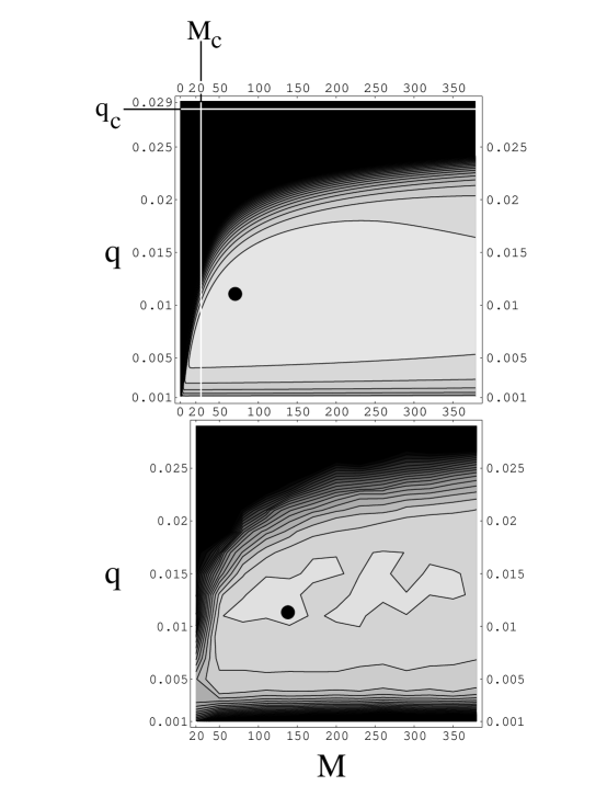
FIG. 5.: Contour plots of the search-effort surface $E(q,M)$ of the average total number of fitness function evaluations for the theory (upper), Eqs. (36) and (41), and for experimental estimates (lower). The parameter settings are $N=4$ blocks of length $K=10$ bits. The population size $M$ runs from $M=1$ to $M=380$ on the horizontal axis on the upper plot and from $M=20$ to $M=380$ on the lower. The mutation rate runs from $q=0.001$ to $q=0.029$ on the vertical. The contours are plotted over the range $E(q,M)=0$ to $E(q,M)=2\times 10^{6}$ with a contour at each multiple of $10^{5}$. The experimental surface was interpolated from $195$ equally spaced data points, $13$ increments of $\Delta M=30$ on the horizontal axis by $15$ increments of $\Delta q=0.002$ on the vertical. The theoretical surface was interpolated over a grid using $\Delta M=1$ and $\Delta q=0.00025$. The optimal theoretical parameter setting, $(q_{o},M_{o})=(0.011,60)$, and the optimal experimental parameter setting, $(q_{o},M_{o})=(0.011,140)$, are marked in their respective plots with a dot.

Note that the error boundary rolls over with increasing $M$ in the upper left corner of the plots. It bends all the way over to the right, eventually running horizontally, thereby determining a population-size independent error threshold. For our parameter settings this occurs around $q\approx 0.028$. Thus, beyond a critical mutation rate of $q_{c}\approx 0.028$ the population almost never discovers the global optimum, even for very large populations.

The value of this horizontal asymptote $q_{c}$ can be roughly approximated by calculating for which mutation rate $q_{c}$ epoch $N$ has exactly the same average fitness as epoch $N-1$; i.e. find $q_{c}$ such that $f_{N}\approx f_{N-1}$. For those parameters, the population is under no selective pressure to move from epoch $N-1$ to epoch $N$. Thus, strings of fitness $N$ will generally not spread in the population. Using our analytic approximations, we find that the critical mutation rate $q_{c}$ is simply given by:

$$q_{c}=1-\sqrt[K]{\frac{N-1}{N}}~{}.$$ (42)

For the parameters of Fig. 5 this gives $q_{c}=0.0284$. This asymptote is indicated there by the horizontal line in the top plot.

Similarly, below a critical population size $M_{c}$, it is also practically impossible to reach the global optimum, even for low mutation rates. This $M_{c}$ can also be roughly approximated by calculating the population size for which the sampling noise is equal to the fitness differential between the last two epochs. We find:

$$M_{c}=\left(\frac{N-1}{N\lambda-N+1}\right)^{2}~{}.$$ (43)

For the parameters of Fig. 5 this gives $M_{c}\approx 27$ around $q=0.011$. This threshold estimate is indicated by the vertical line in Fig. 5.

Further, notice that for small mutation rates, at the bottom of each plot in Fig. 5, the contours run almost horizontally. That is, for small mutation rates relative to the optimum mutation rate $q_{o}$, the total number of fitness function evaluations $E(q,M)$ is insensitive to the population size $M$. Decreasing the mutation rate too far below the optimum rate increases $E(q,M)$ quite rapidly. According to our theoretical predictions it increases roughly as $1/q$ with decreasing $q$. The experimental data indicate that this is a slight underestimation. In fact, $E(q,M)$ appears to increase as $1/q^{\alpha}$ where the exponent $\alpha$ lies somewhere between $1$ and $2$.

Globally, the theoretical analysis and empirical evidence indicate that the search-effort surface $E(q,M)$ is everywhere concave. That is, for any two points $(q_{1},M_{1})$ and $(q_{2},M_{2})$, the straight line connecting these two points is everywhere above the surface $E(q,M)$. We believe that this is always the case for mutation-only genetic algorithms with a static fitness function that has a unique global optimum. This feature is useful in the sense that a steepest descent algorithm on the level of the GA parameters $q$ and $M$ will always lead to the unique optimum $(q_{o},M_{o})$.

Finally, it is important to emphasize once more that there are large run-to-run fluctuations in the total number of fitness evaluations to reach the global optimum. (Recall Table I.) Theoretically, each epoch has an exponentially distributed length since there is an equal and independent innovation probability of leaving it at each generation. The standard deviation of an exponential distribution is equal to its mean. Since the total time $E(q,M)$ is dominated by the last epochs, the total time $E(q,M)$ has a standard deviation close to its mean.

One conclusion from this is that, if one is only going to use a GA for a few runs on a specific problem, there is a large range in parameter space for which the GA’s performance is statistically equivalent. In this sense, fluctuations lead to a large “sweet spot” of GA parameters. On the other hand, these large fluctuations reflect the fact that individual GA runs do not reliably discover the global optimum within a fixed number of fitness function evaluations.

XI Conclusions

We derived explicit analytical approximations to the total number of fitness function evaluations that a GA takes on average to discover the global optimum as a function of both mutation rate and population size. The class of fitness functions so analyzed describes a very general subbasin-portal architecture in genotype space. We found that the GA’s dynamics consists of alternating periods of stasis (epochs) in the fitness distribution of the population, with short bursts of change (innovations) to higher average fitness. During the epochs the most-fit individuals in the population diffuse over neutral networks of isofitness strings until a portal to a network of higher fitness is discovered. Then descendants of this higher fitness string spread through the population.

The time to discover these portals depends both on the fraction of the population that is located on the highest neutral net in equilibrium and the speed at which these population members diffuse over the network. Although increasing the mutation rate increases the diffusion rate of individuals on the highest neutral network, it also increases the rate of deleterious mutations that cause these members “fall off” the highest fitness network. The mutation rate is optimized when these two effects are balanced so as to maximize the total amount of explored volume on the neutral network per generation. The optimal mutation rate, as given by Eq. (22), is dependent on the neutrality degree (the local branching rate) of the highest fitness network and on the fitnesses of the lower lying neutral networks onto which the mutants are likely to fall.

With respect to optimizing population size, we found that the optimal population size occurs when the highest epochs are just barely stable. That is, given the optimal mutation rate, the population size should be tuned such that only a few individuals are located on the highest fitness neutral network. The population size should be large enough such that it is relatively unlikely that all the individuals disappear through a deleterious fluctuation, but not much larger than that. In particular, if the population is much larger, so that many individuals are located on the highest fitness network, then the sampling dynamics causes these individuals to correlate genetically. Due to this genetic correlation, individuals on the highest fitness net do not independently explore the neutral network. This leads, in turn, to a deterioration of the search algorithm’s efficiency. Therefore, the population size should be as low as possible without completely destabilizing the last epochs. Given this, one cannot help but wonder how general the association of efficient search and marginal stability is.

It would appear that the GA wastes computational resources when maintaining a population quasispecies that contains many suboptimal fitness members; that is, those that are not likely to discover higher fitness strings. This is precisely the reason that the GA performs so much more poorly than a simple hill climbing algorithm on this particular set of fitness functions, as shown in Ref. [21]. The deleterious mutations together with the nature of the selection mechanism drives up the fraction of lower fitness individuals in the quasispecies. If we allowed ourselves to tune the selection strength, we could have tuned selection so high that only the most-fit individuals would ever be present. As we will show elsewhere, this leads to markedly better performance, equal to or even slightly exceeding that of hill climbing algorithms. Thus, the GA’s comparatively poor performance is the result of resources being wasted on the presence of suboptimal fitness individuals.

In contrast, the reason that only the best individuals must be kept for optimal search is a result of the fact that our set of fitness functions has no local optima. If there are small fluctuations in fitness on the neutral networks or if there is noise in the fitness function evaluation, it might be beneficial to keep some of the lower fitness individuals in the population. We will also pursue this elsewhere.

For now, it suffices to recall once more the typical dynamical behavior of the GA population around the optimal parameter settings. The GA searches most efficiently when population size and mutation rate are set such that the epochs are marginally stable. That is, the GA dynamics is as “stochastic” as possible without destabilizing the current and later epochs. Strings of fitness $n$ are (only slightly) preferentially reproduced over strings with fitness $n-1$, and the population size is just large enough to protect these fitness $n$ strings from deleterious sampling fluctuations.

More precisely, mutation rate, population size, and network neutralities set a lower bound $\delta f$ of fitness differentials that can be “noticed” by the selection mechanism. This idea is closely related to so called “nearly neutral” theories of molecular evolution of Refs. [23, 24]. For optimal parameter settings, the fitness differential $\delta f=n-(n-1)=1$ is just barely detected by selection. Imagine that during epoch $n$ there are strings which, given an additional $K$ bits set correctly, obtain a fitness $f+\delta f$, instead of $f+1$. As a function of $n$, $K$, $q$ and $M$ we can roughly determine the minimal fitness differential $\delta f$ for these strings to be preferentially selected. We find that

$$\delta f\geq\frac{n}{(1-q)^{K}}\left(\frac{1}{\sqrt{M}}+1-(1-q)^{K}\right).$$ (44)

Below this fitness differential, strings of fitness $f+\delta f$ are effectively neutral with respect to strings with fitness $n$. The net result is that the parameters of the search, such as $q$ and $M$, determine a coarse graining of fitness levels where strings in the band of fitness between $n$ and $n+\delta f$ are treated as having equal fitness.

In future work we explore how this coarse graining can be turned to good use by a GA for fitness functions that possess many shallow local optima—optima that on a coarser scale disappear so that the resulting coarse-grained fitness function induces a neutral network architecture like that explored here. Intuitively, it should be possible to tune GA parameters so that local optima disappear below the minimal fitness differentials $\delta f$ and so that the GA efficiently searches the coarse-grained landscape without becoming pinned to local optima.

A Selection Operator

Since the GA uses fitness-proportionate selection, the proportion $P^{s}_{i}$ of strings with fitness $i$ after selection is proportional to $i$ and to the fraction $P_{i}$ of strings with fitness $i$ before selection; that is, $P^{s}_{i}=c\;i\;P_{i}$. The constant $c$ can be determined by demanding that the distribution remains normalized. Since the average fitness $\langle f\rangle$ of the population is given by Eq. (3), we have $P^{s}_{i}=iP_{i}/{\langle f\rangle}$. In this way, we define a (diagonal) operator ${\bf S}$ that works on a fitness distribution $\vec{P}$ and produces the fitness distribution $\vec{P}^{s}$ after selection by:

$$\left({\bf S}\cdot\vec{P}\right)_{i}=\sum_{j=1}^{N+1}\frac{\delta_{ij}j}{\langle f\rangle}P_{j}~{}.$$ (A1)

Notice that this operator is nonlinear since the average fitness $\langle f\rangle$ is a function of the distribution $\vec{P}$ on which the operator acts.

B Mutation Operator

The component ${\bf M}_{ij}$ of the mutation operator gives the probability that a string of fitness $j$ is turned into a string with fitness $i$ under mutation.

First, consider the components ${\bf M}_{ij}$ with $i<j$. These strings are obtained if mutation leaves the first $i-1$ blocks of the string unaltered and disrupts the $i$th block in the string. Multiplying the probabilities that the preceding $i-1$ blocks remain aligned and that the $i$th block becomes unaligned we have:

$${\bf M}_{ij}=(1-q)^{(i-1)K}\left(1-(1-q)^{K}\right),\;\;i<j~{}.$$ (B1)

The diagonal components ${\bf M}_{jj}$ are obtained when mutation leaves the first $j-1$ blocks unaltered and does not mutate the $j$th block to be aligned. The maximum entropy assumption says that the $j$th block is random and so the probability $P_{a}$ that mutation will change the unaligned $j$th block to an aligned block is given by:

$$P_{a}=\frac{1-(1-q)^{K}}{2^{K}-1}~{}.$$ (B2)

This is the probability that at least one mutation will occur in the block times the probability that the mutated block will be in the correct configuration. Thus, the diagonal components are given by:

$${\bf M}_{jj}=(1-q)^{(j-1)K}(1-P_{a}).$$ (B3)

Finally, we calculate the probabilities for increasing-fitness transitions ${\bf M}_{ij}$ with $i>j$. These transition probabilities depend on the states of the unaligned blocks $j-1$ through $i$. Under the maximum entropy assumption all these blocks are random. The $j$th block is equally likely to be in any of $2^{K}-1$ unaligned configurations. All succeeding blocks are equally likely to be in any one of the $2^{K}$ configurations, including the aligned one. In order for a transition to occur from state $j$ to $i$, all the first $j-1$ aligned blocks have to remain aligned, then the $j$th block has to become aligned through the mutation. The latter has probability $P_{a}$. Furthermore, the following $i-j-1$ blocks all have to be aligned. Finally, the $i$th block has to be unaligned. Putting these together, we find that:

$${\bf M}_{ij} = (1-q)^{(j-1)K}P_{a}$$ (B5)

$$\left(\frac{1}{2^{K}}\right)^{i-j-1}\left(1-\frac{1}{2^{K}}\right)~{},~{}i>j~{}.$$

The last factor does not appear for the special case of the global optimum, $i=N+1$, since there is no $(N+1)$st block.

C Epoch Fitnesses and Quasispecies

The generation operator ${\bf G}$ is given by the product of the mutation and selection operators derived above; i.e. ${\bf G}={\bf M}\cdot{\bf S}$. The operators ${\bf G}^{n}$ are defined as the projection of the operator ${\bf G}$ onto the first $n$ dimensions of the fitness distribution space. Formally:

$${\bf G}^{n}_{i}[\vec{P}]={\bf G}_{i}[\vec{P}],\;\;i\leq n,$$ (C1)

and, of course, the components with $i>n$ are zero.

The epoch quasispecies $\vec{P}^{n}$ is a fixed point of the operator ${\bf G}^{n}$. As in Sec. VI, we take out the factor $\langle f\rangle$ to obtain the matrix ${\bf\tilde{G}}^{n}$. The epoch quasispecies is now simply the principal eigenvector of the matrix ${\bf\tilde{G}}^{n}$ and this can be easily obtained numerically.

However, in order to obtain analytically the form of the quasispecies distribution $\vec{P}^{n}$ during epoch $n$ we approximate the matrix ${\bf\tilde{G}}^{n}$. As shown in App. B, the components ${\bf M}_{ij}$ (and so of ${\bf\tilde{G}}^{n}$) naturally fall into three categories. Those with $i<j$, those with $i>j$, and those on the diagonal $i=j$. Components with $i>j$ involve at least one block becoming aligned through mutation. These terms are generally much smaller than the terms that only involve the destruction of aligned blocks or for which there is no change in the blocks. We therefore approximate ${\bf\tilde{G}}^{n}$ by neglecting terms proportional to the rate of aligned-block creation—what was called $P_{a}$ in App. B. Under this approximation for the components of ${\bf\tilde{G}}^{n}$, we have:

$${\bf\tilde{G}}^{n}_{ij}=j(1-q)^{(i-1)K}(1-(1-q)^{K}),\;\;i<j~{},$$ (C2)

and

$${\bf\tilde{G}}^{n}_{jj}=j(1-q)^{(j-1)K}~{}.$$ (C3)

The components with $i>j$ are now all zero.

Note first that all components of ${\bf\tilde{G}}^{n}$ only depend on $q$ and $K$ through $\lambda\equiv(1-q)^{K}$, the probability that an aligned block is not destroyed by mutation. Note further that in this approximation ${\bf\tilde{G}}^{n}$ is upper triangular. As is well known in matrix theory, the eigenvalues of an upper triangular matrix are given by its diagonal components. Therefore, the average fitness $f_{n}$ in epoch $n$, which is given by the largest eigenvalue, is equal to the largest diagonal component ${\bf\tilde{G}}^{n}$. That is,

$$f_{n}=n(1-q)^{(n-1)K}=n\lambda^{n-1}~{}.$$ (C4)

The principal eigenvector $\vec{P}^{n}$ is the solution of the equation:

$$\sum_{j=1}^{n}\left({\bf\tilde{G}}^{n}_{ij}-f_{n}\delta_{ij}\right)P^{n}_{j}=0~{}.$$ (C5)

Since the components of ${\bf\tilde{G}}^{n}$ depend on $\lambda$ in such a simple way, we can analytically solve for this eigenvector; finding that the quasispecies components are given by:

$$P^{n}_{i}=\frac{(1-\lambda)n\lambda^{n-1-i}}{n\lambda^{n-1-i}-i}\prod_{j=1}^{i-1}\frac{n\lambda^{n-j}-j}{n\lambda^{n-1-j}-j}~{}.$$ (C6)

For the component $P^{n}_{n}$ this reduces to

$$P^{n}_{n}=\prod_{j=1}^{n-1}\frac{n\lambda^{n-j}-j}{n\lambda^{n-1-j}-j}~{}.$$ (C7)

The above equation can be re-expressed in terms of the epoch fitness levels $f_{j}$:

$$P^{n}_{n}=\lambda^{n-1}\prod_{j=1}^{n-1}\frac{f_{n}-f_{j}}{f_{n}-\lambda f_{j}}~{}.$$ (C8)

REFERENCES

- [1] D. Alves and J.F. Fontanari. Error threshold in finite populations. Phys. Rev. E, 57:7008–7013, 1998.
- [2] T. Back. Evolutionary algorithms in theory and practice: Evolution strategies, evolutionary programming, genetic algorithms. Oxford University Press, New York, 1996.
- [3] R. K. Belew and L. B. Booker, editors. Proceedings of the Fourth International Conference on Genetic Algorithms. Morgan Kaufmann, San Mateo, CA, 1991.
- [4] L. Chambers, editor. Practical Handbook of Genetic Algorithms, Boca Raton, 1995. CRC Press.
- [5] L. D. Davis, editor. The Handbook of Genetic Algorithms. Van Nostrand Reinhold, 1991.
- [6] M. Eigen. Self-organization of matter and the evolution of biological macromolecules. Naturwissen., 58:465–523, 1971.
- [7] M. Eigen, J. McCaskill, and P. Schuster. The molecular quasispecies. Adv. Chem. Phys., 75:149–263, 1989.
- [8] M. Eigen and P. Schuster. The hypercycle. A principle of natural self-organization. Part A: Emergence of the hypercycle. Naturwissen., 64:541–565, 1977.
- [9] L. Eshelman, editor. Proceedings of the Sixth International Conference on Genetic Algorithms. Morgan Kaufmann, San Mateo, CA, 1995.
- [10] W. Fontana and P. Schuster. Continuity in evolution: On the nature of transitions. Science, 280:1451–5, 1998.
- [11] S. Forrest, editor. Proceedings of the Fifth International Conference on Genetic Algorithms. Morgan Kaufmann, San Mateo, CA, 1993.
- [12] C. W. Gardiner. Handbook of Stochastic Methods. Springer-Verlag, 1985.
- [13] D. E. Goldberg. Genetic Algorithms in Search, Optimization, and Machine Learning. Addison-Wesley, Reading, MA, 1989.
- [14] M. Huynen, P. F. Stadler, and W. Fontana. Smoothness within ruggedness: The role of neutrality in adaptation. Proc. Natl. Acad. Sci., 93:397–401, 1996.
- [15] M. A. Huynen. Exploring phenotype space through neutral evolution. J. Mol. Evol., 43:165–169, 1995.
- [16] M. Kimura. Diffusion models in population genetics. J. Appl. Prob., 1:177–232, 1964.
- [17] M. Kimura. The neutral theory of molecular evolution. Cambridge University Press, 1983.
- [18] J. R. Koza. Genetic programming: On the programming of computers by means of natural selection. MIT Press, Cambridge, MA, 1992.
- [19] I. Leuthaüsser. Statistical mechanics of Eigen’s evolution model. J. Stat. Phys., 48:343–360, 1987.
- [20] M. Mitchell. An Introduction to Genetic Algorithms. MIT Press, Cambridge, MA, 1996.
- [21] M. Mitchell, J. H. Holland, and S. Forrest. When will a genetic algorithm outperform hill climbing?, 1994. In J. D. Cowan, G. Tesauro, and J. Alspector (editors), Advances in Neural Information Processing Systems 6. San Mateo, CA: Morgan Kaufmann.
- [22] M. Nowak and P. Schuster. Error thresholds of replication in finite populations, Mutation frequencies and the onset of Muller’s ratchet. J. Theo. Bio., 137:375–395, 1989.
- [23] T. Ohta. Slightly deleterious mutant substitutions in evolution. Nature, 247:96–98, 1973.
- [24] T. Ohta and J.H. Gillespie. Development of neutral and nearly neutral theories. Theo. Pop. Bio., 49:128–142, 1996.
- [25] A. Prügel-Bennett and J. L. Shapiro. Analysis of genetic algorithms using statistical mechanics. Phys. Rev. Lett., 72(9):1305–1309, 1994.
- [26] A. Prügel-Bennett and J. L. Shapiro. The dynamics of a genetic algorithm in simple random Ising systems. Physica D, 104 (1):75–114, 1997.
- [27] M. Rattray and J. L. Shapiro. The dynamics of a genetic algorithm for a simple learning problem. J. of Phys. A, 29(23):7451–7473, 1996.
- [28] C. M. Reidys, C. V. Forst, and P. K. Schuster. Replication and mutation on neutral networks of RNA secondary structures. Bull. Math. Bio., 1998. submitted, Santa Fe Institute Working Paper 98-04-36.
- [29] J. Swetina and P. Schuster. Self replicating with error, A model for polynucleotide replication. Biophys. Chem., 16:329–340, 1982.
- [30] E. van Nimwegen and J. P. Crutchfield. Optimizing epochal evolutionary search: Population-size independent theory. Computer Methods in Applied Mechanics and Engineering, special issue on Evolutionary and Genetic Algorithms in Computational Mechanics and Engineering, D. Goldberg and K. Deb, editors, submitted, 1998. Santa Fe Institute Working Paper 98-06-046.
- [31] E. van Nimwegen, J. P. Crutchfield, and M. Mitchell. Finite populations induce metastability in evolutionary search. Phys. Lett. A, 229:144–150, 1997.
- [32] E. van Nimwegen, J. P. Crutchfield, and M. Mitchell. Statistical dynamics of the Royal Road genetic algorithm. Theoretical Computer Science, special issue on Evolutionary Computation, A. Eiben and G. Rudolph, editors, in press, 1998. SFI working paper 97-04-35.
- [33] J. Weber. Dynamics of Neutral Evolution. A case study on RNA secondary structures. PhD thesis, Biologisch-Pharmazeutischen Fakultät der Friedrich Schiller-Universität Jena, 1996.
- [34] D. H. Wolpert and W. G. Macready. No free lunch theorems for optimization. IEEE Trans. Evol. Comp., 1:67–82, 1997.