Optimizing Epochal Evolutionary Search:
Population-Size Independent Theory

Abstract

Epochal dynamics, in which long periods of stasis in population fitness are punctuated by sudden innovations, is a common behavior in both natural and artificial evolutionary processes. We use a recent quantitative mathematical analysis of epochal evolution to estimate, as a function of population size and mutation rate, the average number of fitness function evaluations to reach the global optimum. This is then used to derive estimates of and bounds on evolutionary parameters that minimize search effort.

Santa Fe Institute Working Paper 98-06-046

Contents

toc

I Engineering Evolutionary Search

Evolutionary search refers to a class of stochastic optimization techniques—loosely based on processes believed to operate in biological evolution—that have been applied successfully to a variety of different problems; see, for example, Refs. [2, 4, 6, 9, 14, 17, 26] and references therein. Unfortunately, the mechanisms constraining and driving the dynamics of evolutionary search on a given problem are not well understood. In mathematical terms evolutionary search algorithms are nonlinear population-based stochastic dynamical systems. The complicated dynamics exhibited by such systems has been appreciated for decades in the field of mathematical population genetics. For example, the effects on evolutionary behavior of the rate of genetic variation, the population size, and the function to be optimized typically cannot be analyzed separately; there are strong, nonlinear interactions between them. These complications make an empirical approach to the question of whether and how to use evolutionary search problematic. The lack of a unified theory has rendered the literature largely anecdotal and of limited generality. The work presented here continues an attempt to unify and extend theoretical work that has been done in the areas of evolutionary search theory, molecular evolution theory, and mathematical population genetics. The goal is to obtain a more general and quantitative understanding of the emergent mechanisms that control the dynamics of evolutionary search and other population-based dynamical systems.

Our approach takes a structural view of the search space and solves the population dynamics as it is constrained by a general architecture for epochal evolution—a class of population dynamics in which long periods of stasis are punctuated by rapid innovations. Based on a phenotypically induced decomposition, the genome space is broken into strongly and weakly connected sets. From this we motivate several simplifying assumptions that lead to the class of fitness functions and genetic operators we analyze. Stated in the simplest possible terms, all of the resulting population dynamical behavior derives from the interplay of the architecture, the infinite-population nonlinear dynamics, and the stochasticity arising from finite-population sampling.

One might object that important details of real biological evolution, on the one hand, or of alternative evolutionary search algorithms, on the other hand, are not described by the resulting class of evolutionary dynamical systems. Our response is simple: One must start somewhere. The bottom line is that the results and their predictive power justify the approach. Moreover, along the way we come to appreciate a number of fundamental trade-offs and basic mechanisms that drive and inhibit evolutionary search.

Our results show that a detailed dynamical understanding, announced in Ref. [36] and expanded in Ref. [37], can be turned to a very practical advantage. Specifically, we determine how to set population size and mutation rate to reach, in the fewest steps, the global optimum in a wide class of fitness functions. In other words, our objective is to minimize the total number of fitness function evaluations as a function of evolutionary search parameters.

Our analysis provides several insights that are useful knowledge for engineers even in much more complicated optimization problems (and, for that matter, for the theory of evolutionary dynamics in biology). Using these, in a sequel we draw some conclusions about those optimization problems for which population-based search methods, such as genetic algorithms and genetic programming (to mention only two examples), are appropriate.

II Landscape Architecture

The fitness functions characteristic of problems that evolutionary search or (say) simulated annealing are being used for in practice are very complicated, almost by definition. On the one hand, detailed knowledge of the fitness function implies that one does not need to run an optimization method to find high fitness solutions. On the other hand, assuming no structure at all leads to a completely random fitness function for which it is known that any optimization algorithm performs as well on average as random search [41]. Not surprisingly, reality is a middle ground.

Therefore, our strategy to understand the workings of evolutionary search algorithms is to assume some structure in the fitness function that is germane to search population dynamics and to assume that, beyond this, there is no other structure. That is, apart from the structure we impose, the fitness function is as unstructured as can be.

There is a concomitant and compelling biological motivation for our choice of architecture. This is the common occurrence in natural evolutionary systems of “punctuated equilibria”—a process first introduced to describe sudden morphological changes in the paleontological record [19]. Similar behavior has been recently studied experimentally in bacterial colonies [13] and in simulations of the evolution of transfer-RNA secondary structure [15]. It has been argued, moreover, that punctuated dynamics occurs at both genotypic and phenotypic levels [5]. This class of behavior appears robust enough to also occur in artificial evolutionary systems, such as evolving cellular automata [8, 28] and populations of competing programs [1].

How are we to think of the mechanisms that cause this evolutionary behavior? The evolutionary biologist Wright introduced the notion of “adaptive landscapes” to describe the (local) stochastic adaptation of populations to themselves and to environmental constraints [42]. This geographical metaphor has had a powerful influence on thinking about natural and artificial evolutionary processes. The basic picture is that evolutionary dynamics stochastically crawls along a surface determined, perhaps dynamically, by the fitness of individuals, moving to peaks and very occasionally hopping across fitness “valleys” to nearby, and hopefully higher fitness, peaks.

More recently, it has been assumed that the typical fitness functions of combinatorial optimization and biological evolution can be modeled as “rugged landscapes” [24, 27]. These are functions with wildly fluctuating fitnesses even at the smallest scales of single-point mutations. The result is that these “landscapes” possess a large number of local optima.

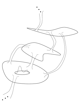
FIG. 1.: Subbasin and portal architecture underlying epochal evolution. Roughly speaking, a population diffuses in the subbasins (large sets) until a portal (a tube) to a higher fitness subbasin is found.

At the same time an increasing appreciation has developed, in marked contrast to this rugged landscape view, that there are substantial degeneracies in the genotype-to-phenotype and the phenotype-to-fitness mappings. The crucial role played by these degeneracies has found important applications in molecular evolution; e.g. see Ref. [16]. Up to small fluctuations, when these degeneracies are operating the number of distinct fitness values in the landscape is often much smaller than the number of genotypes. Moreover, due to the high dimensionality of these genotype spaces, sets of genotypes with approximately equal fitness tend to form components in genotype space that are connected by single mutational steps. Finally, due to intrinsic or even exogenous effects (e.g. environmental) there simply may not exist a “fitness” value for each genotype. Fluctuations can induce variation in fitness such that genotypes with neighboring fitness values are not distinct at the level of selection. A similar effect can also arise when a fast rate of change does not allow subtle distinctions in fitness to become manifest.

When these biological facts are taken into account we end up with an alternative view to both Wright’s “adaptive” landscapes and the more recent “rugged” landscapes. That is, the fitness landscape decomposes into a set of “neutral networks” of approximately isofitness genotypes that are entangled with each other in a complicated and largely unstructured fashion; see Fig. 1. Within each neutral network selection is effectively disabled and neutral evolution dominates. Some of the first steps in understanding the consequences of neutral evolution (in single neutral networks) were taken by Kimura in the 1960’s using stochastic process analyzes adopted from statistical physics [25]. Despite the early progress in neutral evolution, a number of fundamental problems remain [10]. Although we will analyze neutral evolution in the following, we also emphasize the global architectural structure that connects the neutral networks and drives and constrains epochal evolutionary search.

This intuitive view of biologically plausible fitness landscapes—as a relatively small number of connected neutral nets—is the one that we adopt in the following analysis. We formalize it by making several more specific assumptions about the fitness function. First, we assume that there are $N+1$ different neutral nets, with fitnesses $1,2,\ldots,N+1$. Second, we assume that the higher the fitness, the smaller the isofitness neutral net volume. That is, there are fewer strings of high fitness than low. More specifically, we assume that the proportion of genotype space that is occupied by strings of fitness $n$ scales as $2^{-Kn}$, where $K$ is a measure of the rate at which the proportion of higher fitness strings decreases with fitness level. Finally, we assume that strings with fitness $n+1$ can be reached by a single point mutation from strings with fitness $n$. Specifically, we assume that the set of strings with fitness $n+1$ is a subspace of the set of strings with fitness $n$. The resulting architecture is a modified version of the general subbasin-portal structure of Fig. 1 and is illustrated in Fig. 2; after Ref. [7].

Why assume that strings of higher fitness are nested inside those of lower fitness? We believe that this assumption is consonant, by definition, with the very idea of using evolutionary search for optimization. Imagine, on the contrary, that strings of fitness $n+1$ are more likely to be close to strings with fitness $n-1$ than to those of fitness $n$. It then seems strange to have selection preferably replicate strings of fitness $n$ over strings with fitness $n-1$. One result is that this leads to an increased (ineffective) search effort centered around strings of fitness $n$. Therefore, designing a search algorithm to select the current best strings implicitly assumes that strings of higher fitness tend to be found close to strings of the current best fitness.

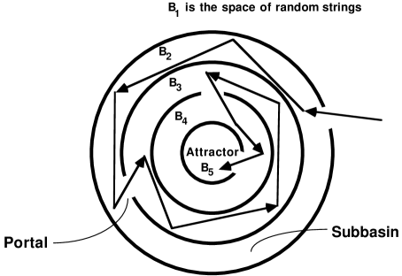
FIG. 2.: The dimensional hierarchy of subbasins and portals for the Royal Staircase fitness functions.

In this way we shift our view away from the geographic metaphor of evolutionary search “crawling” along a fixed and static (smooth or rugged) “landscape” to that of a diffusion process constrained by the subbasin-portal architecture induced by degeneracies in the genotype-to-phenotype and phenotype-to-fitness mappings. Moreover, as will become more apparent, our approach is not just a shift in architecture, but it also focuses on the dynamics of populations as they move through the subbasins to find portals to higher fitness. A side benefit is that it does not limit itself to evolutionary processes for which a potential function exists; as the landscape analyses do.

III The Royal Staircase Fitness Function

Under the above assumptions, the class of fitness functions, referred to as the “Royal Staircase”, delineated is equivalent to the following specification:

1. Genomes are specified by binary strings $s=s_{1}s_{2}\cdots s_{L},s_{i}\in\{0,1\},$ of length $L=NK$.

2. Reading the genome from left to right, the number $I(s)$ of consecutive $1$s is counted.

3. The fitness $f(s)$ of string $s$ with $I$ consecutive ones, followed by a zero, is $f(s)=1+\lfloor I(s)/K\rfloor$. The fitness is thus an integer between $1$ and $N+1$.

4. The (single) global optimum is the genome $s=1^{L}$; namely, the string of all $1$s.

From this it is easy to see that we have chosen $N$ (consecutive) sets of $K$ bits to represent the different fitness classes. These sets we call “blocks”. The first block consists of the first $K$ bits on the left, i.e. $s_{1}\cdots s_{K}$. The second block consists of bits $s_{K+1}\cdots s_{2K}$ and so on. For each of these blocks there is one “aligned” configuration consisting of $K$ $1$s and $2^{K}-1$ “unaligned” configurations. If the first block is unaligned, the string obtains fitness $1$. If the first block is aligned and the second unaligned, it obtains fitness $2$. If the first two blocks are aligned and the third unaligned, it obtains fitness $3$, and so on up to the globally optimal string with all aligned blocks and fitness $N+1$.

Without affecting the evolutionary dynamics or the underlying architecture of genotype space, we could have chosen a different “aligned” block than the all-$1$s configuration. In fact, we could have chosen different aligned configurations for the different blocks and still not affected the dynamics. Furthermore, since we will not be analyzing crossover, we could have chosen the locations of the bits of each block to be anywhere in the genome without affecting the dynamics. The only constraint, other than the block’s ordering, is that we have $N$ disjoint sets of $K$ bits.

Notice further that the proportion $\rho_{n}$ of strings with fitness $n$ is given by:

$$\rho_{n}=2^{-K(n-1)}\left(1-2^{-K}\right)~{}.$$ (1)

The net result is that this fitness function implements the intuitive idea that increasing fitness is obtained by setting more and more bits correctly. One can only set correct bit values in sets of $K$ bits at a time and in blocks from left to right. (Due to the modularity of the subbasin-portal architecture, and of the resulting theory we present below, the restriction to uniform block size also could be lifted.) A genome’s fitness is proportional to the number of blocks it has set correctly. This realizes our view of the underlying architecture as a set of isofitness genomes that occur in nested neutral networks of smaller and smaller volume; as shown in Fig. 2.

IV The Genetic Algorithm

For our analysis of evolutionary search we have chosen a simplified form of a genetic algorithm (GA) that does not include crossover and that uses fitness-proportionate selection. The GA is defined by the following steps.

1. Generate a population of $M$ bit strings of length $L=NK$ with uniform probability over the space of $L$-bit strings.

2. Evaluate the fitness of all strings in the population.

3. Stop the algorithm, noting the generation number $t_{\rm opt}$, if a string with optimal fitness $N+1$ occurs in the population. Else, proceed.

4. Create a new population of $M$ strings by selecting, with replacement and in proportion to fitness, strings from the current population.

5. Mutate each bit in each string of the new population with probability $q$.

6. Go to step 2.

The total number $E$ of fitness function queries is $E=Mt_{\rm opt}$. We are interested in the average number $E$ of queries per GA run required over a large number $R$ of runs. Note that the average total amount of mutational information introduced into the populations during a single GA run is $qNKMt_{\rm opt}$.

The main motivation for leaving out crossover is that this greatly simplifies our analysis. The benefit is that we can make detailed quantitative predictions of the GA’s behavior. Moreover, we believe that, from the point of view of optimization, the addition of crossover to the genetic operators only marginally improves the efficiency of the search. We comment on this, which admittedly is at variance with common beliefs about evolutionary search, later on. Additional discussion and supporting evidence can be found in section 6.5 of Ref. [37] and in Ref. [28].

Notice that our GA effectively has two parameters: the mutation rate $q$ and the population size $M$. A given search problem is specified by the fitness function in terms of $N$ and $K$. The central goal of the following analysis is to find those settings of $M$ and $q$ that minimize the number $E$ of fitness function queries for given $N$ and $K$.

V Observed Population Dynamics

The typical dynamics of a population evolving on a landscape of connected neutral networks, such as defined above, alternates between long periods of stasis in the population’s average fitness (“epochs”) and sudden increases in the average fitness (“innovations”). (See, for example, Fig. 1 of Ref. [37].) As was first pointed out in the context of molecular evolution in Ref. [23], the best individuals in the population diffuse over the neutral network (“subbasin”) of isofitness genotypes until one of them discovers a connection (“portal”) to a neutral network of even higher fitness. The fraction of individuals on this new network then grows rapidly, reaching an equilibrium after which the new subset of most-fit individuals diffuses again over the new neutral network. In addition to the increasing attention paid to this type of epochal evolution in the theoretical biology community [18, 22, 29, 34, 40], recently there has also been an increased interest by evolutionary search theorists [3, 20].

The GA just defined is the same as that studied in our earlier analyses [36, 37]. Also, the Royal Staircase fitness function defined above is very similar to the “Royal Road” fitness function that we used there. It should not come as a surprise, therefore, that qualitatively the GA’s experimentally observed behavior is very similar to that reported in Refs. [36] and [37]. Moreover, most of the theory developed there for epochal evolutionary dynamics carries over to the Royal Staircase class of fitness functions.

We now briefly recount the experimentally observed behavior of typical Royal Staircase GA runs. The reader is referred to Ref. [37] for a detailed discussion of the dynamical regimes this type of GA exhibits under a range of different parameter settings.

FIG. 3.: Examples of the Royal Staircase GA population dynamics with different parameter settings. The four plots show best fitness in the population (upper lines) and average fitness in the population (lower lines) as a function of time, measured in generations. The fitness function and GA parameters are given in each plot. In each case we have chosen $q$ and $M$ in the neighborhood of their optimal settings (see later) for each of the four values of $N$ and $K$.

Figure 3 shows the GA’s behavior with four different parameter settings. The vertical axes show the best fitness in the population (upper lines) and the average fitness in the population (lower lines) as a function of the number of generations. Each figure is produced from a single GA run. In all of these runs the average fitness $\langle f\rangle$ in the population goes through stepwise changes early in the run, alternating epochs of stasis with sudden innovations in fitness. Later in the run, the average fitness tends to have higher fluctuations. Notice also that $\langle f\rangle$ roughly tracks the epochal behavior of the best fitness in the population. Notice, too, that often the best fitness shows a series of innovations to higher fitness that are lost. Eventually these innovations “fixate” in the population. Finally, for each of the four settings of $N$ and $K$ we have chosen the values of $M$ and $q$ such that the total number $E$ of fitness function evaluations to reach the global optimum for the first time is roughly minimal. Thus, the four plots illustrate the GA’s typical dynamics close to optimal $(M,q)$-parameter settings—the analysis for which begins in the next section.

There is a large range, almost a factor of $10$, in times to reach the global optimum across the runs. Thus, there can be a strong parameter dependence in search times. Moreover, the variance of the total number $E$ of fitness function evaluations is the same size as the average $E$. Thus, there are large run-to-run variations in the time to reach the global optimum, even with the parameters held constant. This is true for all parameter settings with which we experimented, of which only a few are reported here.

Figure 3(a) plots the results of a GA run with $N=8$ blocks of $K=8$ bits each, a mutation rate of $q=0.006$, and a population size of $M=200$. During the epochs, the best fitness in the population jumps up and down several times before it finally jumps up and the new more-fit string stabilizes in the population. This transition is reflected in the average fitness also starting to move upward. In this particular run, it took the GA approximately $3\times 10^{5}$ fitness function evaluations to reach the global optimum for the first time. Over 250 runs the GA takes on average $5\times 10^{5}$ fitness function evaluations to reach the global optimum for these parameters. The inherent large per-run variation means in this case that some runs take less than $10^{5}$ function evaluations and that others take many more than $10^{6}$.

Figure 3(b) plots a run with $N=6$ blocks of length $K=6$ bits, a mutation rate of $q=0.012$, and a population size of $M=150$. The GA reached the global optimum after approximately $3\times 10^{4}$ fitness function evaluations. On average, the GA uses approximately $5\times 10^{4}$ fitness function evaluations to reach the global fitness optimum. Notice that somewhere after generation $500$ the global optimum is lost again from the population. It turns out that this is a typical feature of the GA’s behavior for parameter settings close to those that give minimal $E$. The global fitness optimum often only occurs in relatively short bursts after which it is lost again from the population. Notice also that there is only a small difference in $\langle f\rangle$ depending whether the best fitness is either $6$ or $7$.

Figure 3(c) shows a run for a small number ($N=4$) of large ($K=10$) blocks. The mutation rate is $q=0.01$ and the population size is again $M=150$. As in all three other runs we see that the average fitness goes through epochs punctuated by rapid increases of average fitness. We also see that the best fitness in the population jumps up several times before the population fixates on a higher fitness. The GA takes about $2\times 10^{5}$ fitness function evaluations on average to reach the global optimum for these parameter settings. In this run, the GA just happened to have taken about $2.5\times 10^{5}$ fitness function evaluations.

Finally, Fig. 3(d) shows a run with a large number ($N=10$) of smaller ($K=5$) blocks. The mutation rate is $q=0.008$ and the population size is $M=100$. Notice that in this run, the best fitness in the population alternates several times between fitnesses $7$, $8$, and $9$ before it reaches the global fitness optimum of $11$. After it has reached the global optimum for several time steps, the global optimum disappears again and the best fitness in the population alternates between $9$ and $10$ from then on. It is notable that this intermittent behavior of the best fitness is barely discernible in the behavior of the average fitness. It appears to be lost in the “noise” of the average fitness fluctuations. The GA takes about $10^{5}$ fitness function evaluations on average at these parameter settings to reach the global optimum; while in this particular run the GA took only $6\times 10^{4}$ fitness function evaluations.

Again, we stress that there are large fluctuations in the total number of fitness evaluations to reach the global optimum between runs. One tentative conclusion is that, if one is only going to use a GA for a few runs on a specific problem, there is a large range in parameter space for which the GA’s performance is statistically equivalent. On the one hand, the large fluctuations in the GA’s search dynamics make it hard to predict for a single run how long it is going to take to reach the global optimum. On the other hand, this prediction is largely insensitive to the precise parameter settings in a ball centered around the optimal parameter settings. Thus, the large fluctuations lead to a large “sweet spot” of GA parameters, but the GA does not reliably discover the global optimum within a fixed number of fitness function evaluations.

VI Statistical Dynamics of Evolutionary Search

In Refs. [36] and [37] we developed the statistical dynamics of genetic algorithms to analyze the behavioral regimes of a GA searching the Royal Road fitness function. The analysis here builds on those results. Due to the strong similarities we will only briefly introduce this analytical approach to evolutionary dynamics. The reader is referred to Ref. [37] for an extensive and detailed exposition. There the reader also will find a review of the alternative methodologies for GA theory developed by Vose and collaborators [30, 38, 39], by Prugell-Bennett, Rattray, and Shapiro[31, 32, 33], and in mathematical population genetics.

From a microscopic point of view, the state of an evolving population is only fully described when a list $\cal{S}$ of all genotypes with their frequencies of occurrence in the population is given. The evolutionary dynamics is implemented via the conditional transition probabilities $P(\cal{S^{\prime}}|\cal{S})$ that the population at the next generation will be the microscopic state $\cal{S^{\prime}}$. For any reasonable genetic representation, there will be an enormous number of these microscopic states $\cal{S}$ and their transition probabilities. This makes it almost impossible to quantitatively study the dynamics at this microscopic level.

More practically, a full description of the dynamics on the level of microscopic states $\cal{S}$ is neither useful nor typically of interest. One is much more likely to be concerned with relatively coarse statistics of the dynamics, such as the evolution of the best and average fitness in the population or the waiting times for evolution to produce a string of a certain quality. The result is that quantitative mathematical analysis faces the task of finding a description of the evolutionary dynamics that is simple enough to be tractable numerically or analytically and that, moreover, facilitates the prediction the quantities of interest to a practitioner.

With these issues in mind, we specify the state of the population at any time by some relatively small set of “macroscopic” variables. Since this set of variables intentionally ignores vast amounts of microscopic detail, it is generally impossible to exactly describe the GA’s dynamics in terms of these macroscopic variables. In order to acheive the benefits of a coarser description, however, we assume that given the state of the macroscopic variables, the population has equal probabilities to be in any of the microscopic states consistent with the specified state of the macroscopic variables. This “maximum entropy” assumption lies at the heart of statistical mechanics in physics.

We assume in addition that in the limit of infinite population size, the resulting equations of motion for the macroscopic variables become closed. That is, for infinite populations, we assume that we can exactly predict the state of the macroscopic variables at the next generation, given the present state of the macroscopic variables. This limit is analogous to the thermodynamic limit in statistical mechanics; the corresponding assumption is analogous to “self-averaging” of the dynamics in this limit.

The key, and as yet unspecified step, in developing such a thermodynamic model of evolutionary dynamics is to find an appropriate set of macroscopic variables that satisfies the above assumptions. In practice this is difficult. Ultimately, the suitability of a set of macroscopic variables has to be verified by comparing theoretical predictions with experimental measurements. In choosing such a set of macroscopic variables one is guided by our knowledge of the fitness function and the search’s genetic operators.

To see how this choice is made imagine that strings can have only two possible values for fitness, $f_{A}$ and $f_{B}$. Assume also that under mutation all strings of type $A$ are equally likely to turn into type-$B$ strings and that all strings of type $B$ have equal probability to turn into strings of type $A$. In this situation, it is easy to see that we can take the macroscopic variables to be the relative proportions of $A$ strings and $B$ strings in the population. Any additional microscopic detail, such as the number of $1$s in the strings, is not required or relevant to the evolutionary dynamics. Neither selection nor mutation distinguish different strings within the sets $A$ and $B$ on the level of the proportions of $A$’s and $B$’s they produce in the next generation.

Similarly, our approach describes the state of the population at any time only by the distribution of fitness in the population. That is, we group strings into equivalence classes of equal fitness and assume that, on the level of the fitness distribution, the dynamics treats all strings within a fitness class as equal. At the macroscopic (fitness) level of the dynamics, we know that a string of fitness $n$ has the first $n-1$ blocks aligned and the $n$th block in one of the $2^{K}-1$ other unaligned configurations. The maximum entropy assumption specifies that for all strings of fitness $n$, the $n$th block is equally likely to be in any of the $2^{K}-1$ unaligned configurations and that each of the blocks $n+1$ through $N$ are equally likely to be in any of their possible $2^{K}$ block configurations.

Various reasons suggest the maximum entropy approximation will not be valid in practice. For example, the fixation due to finite population size makes it hard to believe that all unaligned block configurations in all strings are random and independent. For large populations, fortunately, the assumption is compelling. In fact, in the limit of very large population sizes, typically $M>2^{L}$, the GA’s dynamics on the level of fitness distributions accurately captures the fitness distribution dynamics found experimentally [37]. In any case, we will solve explicitly for the fitness distribution dynamics in the limit of infinite populations using our maximum entropy assumption and then show how this solution can be used to solve for the finite-population dynamics.

The essence of our statistical dynamics approach then is to describe the population state at any time during a GA run by a relatively small number of macroscopic variables—variables that in the limit of infinite populations self-consistently describe the dynamics at their own level. After obtaining this infinite population dynamics explicitly, we then use it to solve for the GA’s dynamical behaviors with finite populations.

Employing the maximum entropy principle and focusing on fitness distributions is also found in an alternative statistical mechanics approach to GA dynamics developed by Prug̈el-Bennett, Rattray, and Shapiro [31, 32, 33]. In their approach, however, maximum entropy is assumed with respect to the ensemble of entire GA runs. Specifically, in their analysis the average dynamics, averaged over many runs, of the first few cumulants of the fitness distribution are predicted theoretically. The result is that almost all of the relevant behavior, e.g. as illustrated in Fig. 3 of the previous section, is averaged away. In contrast, our statistical dynamics approach applies maximum entropy only to the population’s current state, given its current fitness distribution. The result is that for finite populations we do not assume that the GA dynamics is self-averaging. That is, two runs, with equal fitness distributions $\vec{P}$ at time $t$, are not assumed to have the same future macroscopic behavior. They are assumed only to have the same probability distribution of possible futures.

A Generation Operator

The macroscopic state of the population is determined by its fitness distribution, denoted by a vector $\vec{P}=\{P_{1},P_{2},\ldots,P_{N+1}\}$, where the components $0\leq P_{n}\leq 1$ are the proportion of individuals in the population with fitness $n=1,2,\ldots,N+1$. We refer to $\vec{P}$ as the phenotypic quasispecies, following its analog in molecular evolution theory [11, 12]. Since $\vec{P}$ is a distribution, we have the normalization condition:

$$\sum_{n=1}^{N+1}P_{n}=1.$$ (2)

The average fitness $\langle f\rangle$ of the population is given by:

$$\langle f\rangle=\sum_{n=1}^{N+1}nP_{n}.$$ (3)

In the limit of infinite populations and under our maximum entropy assumption, we can construct a generation operator ${\bf G}$ that maps the current fitness distribution $\vec{P}(t)$ deterministically into the fitness distribution $\vec{P}(t+1)$ at the next time step; that is,

$$\vec{P}(t+1)={\bf G}[\vec{P}(t)]~{}.$$ (4)

The operator ${\bf G}$ consists of a selection operator ${\bf S}$ and a mutation operator ${\bf M}$:

$${\bf G}={\bf M}\cdot{\bf S}.$$ (5)

The selection operator encodes the fitness-level effect of selection on the population; and the mutation operator, the fitness-level effect of mutation. Below we construct these operators for our GA and the Royal Staircase fitness function explicitly. For now we note that the infinite population dynamics can be obtained by iteratively applying the operator ${\bf G}$ to the initial fitness distribution $\vec{P}(0)$. Thus, the macroscopic equations of motion are formally given by

$$\vec{P}(t)={\bf G}^{(t)}[\vec{P}(0)]~{}.$$ (6)

Recalling Eq. (1) it is easy to see that the initial fitness distribution $\vec{P}(0)$ is given by:

$$P_{n}(0)=2^{-K(n-1)}\left(1-2^{-K}\right)\;,~{}1\leq n\leq N~{},$$ (7)

and

$$P_{N+1}(0)=2^{-KN}.$$ (8)

As shown in Refs. [36] and [37], despite ${\bf G}$’s nonlinearity, it can be linearized such that the $t$th iterate ${\bf G}^{(t)}$ can be directly obtained by solving for the eigenvalues and eigenvectors of ${\bf G}$.

For very large populations ($M>2^{L}$) the dynamics of the fitness distribution obtained from GA simulation experiments is accurately predicted by iteration of the operator ${\bf G}$. It is noteworthy, though, that this “infinite” population dynamics is qualitatively very different from the behavior shown in Fig. 3. For large populations strings of all fitnesses are present in the initial population and the average fitness increases smoothly and monotonically to an asymptote over a small number of generations. (This limit is tantamount to an exhaustive search, requiring as it does ${\cal O}(2^{L})$ fitness function evaluations.) Despite this seeming lack of utility, in the next section we show how to use the infinite population dynamics given by ${\bf G}$ to describe the finite-population behavior.

B Finite Population Dynamics

There are two important differences between the infinite-population dynamics and that with finite populations. The first is that with finite populations the components $P_{n}$ cannot take on arbitrary values between $0$ and $1$. Since the number of individuals with fitness $n$ in the population is necessarily integer, the values of $P_{n}$ are quantized to multiples of $1/M$. The space of allowed finite population fitness distributions thus turns into a regular lattice in $N+1$ dimensions with a lattice spacing of $1/M$ within the simplex specified by normalization (Eq. (2)). Second, the dynamics of the fitness distribution is no longer deterministic. In general, we can only determine the conditional probabilities ${\rm Pr}[\vec{Q}|\vec{P}]$ that a certain fitness distribution $\vec{P}$ leads to another $\vec{Q}$ in the next generation.

Fortunately, the probabilities ${\rm Pr}[\vec{Q}|\vec{P}]$ are simply given by a multinomial distribution with mean ${\bf G}[\vec{P}]$, which in turn is the result of the action of the infinite population dynamics. This can be understood in the following way. In creating the population for the next generation individuals are selected, copied, and mutated, $M$ times from the same population $\vec{P}$. This means that for each of the $M$ selections there are equal probabilities that a string of fitness $n$ will be produced in the next generation. For an infinite number of selections the final proportions $Q_{n}$ of strings with fitness $n$ are just the probabilities to produce a single individual with fitness $n$ with a single selection. That is, given an infinite population ${\bf G}[\vec{P}]$ we have for a finite population that the fitness distribution $\vec{Q}$ is a random sample of size $M$ of the distribution ${\bf G}[\vec{P}]$.

Putting these observations together, if we write $Q_{n}=m_{n}/M$, with $0\leq m_{n}\leq M$ being integers, we have:

$${\rm Pr}[\vec{Q}|\vec{P}]=M!\prod_{n=1}^{N+1}\frac{\left({\bf G}_{n}[\vec{P}]\right)^{m_{n}}}{m_{n}!}~{}.$$ (9)

We see that for any finite-population fitness distribution $\vec{P}$ the operator ${\bf G}$ still gives the GA’s average dynamics over one time step, since the expected fitness distribution at the next time step is ${\bf G}[\vec{P}]$. Note that the components ${\bf G}_{n}[\vec{P}]$ need not be multiples of $1/M$. Therefore the actual fitness distribution $\vec{Q}$ at the next time step is not ${\bf G}[\vec{P}]$, but is instead one of the lattice points of the finite-population state space. Since the variance around the expected distribution ${\bf G}[\vec{P}]$ is proportional to $1/M$, $\vec{Q}$ is likely to be close to ${\bf G}[\vec{P}]$.

C Epochal Dynamics

For finite populations, the expected change $\langle d\vec{P}\rangle$ in the fitness distribution over one generation is given by:

$$\langle d\vec{P}\rangle={\bf G}[\vec{P}]-\vec{P}.$$ (10)

Assuming that some component $\langle dP_{i}\rangle$ is much smaller than $1/M$, the actual change in component $P_{i}$ is likely to be $dP_{i}=0$ for a long succession of generations. That is, if the size of the “flow” $\langle dP_{i}\rangle$ in some direction $i$ is much smaller than the lattice spacing ($1/M$) for the finite population, we expect the fitness distribution to not change in direction (fitness) $i$. In Refs. [36] and [37] we showed that this is the mechanism that causes epochal dynamics for finite populations. More formally, each epoch $n$ of the dynamics corresponds to the population being restricted to a region in the $n$-dimensional lower-fitness subspace of fitnesses $1$ to $n$ of the macroscopic state space. Stasis occurs because the flow out of this subspace is much smaller than the finite-population induced lattice spacing.

As Fig. 3 illustrates, each epoch in the average fitness is associated with a constant value of the best fitness in the population. More detailed experiments reveal that not only is $\langle f\rangle$ constant on average during the epochs, in fact the entire fitness distribution $\vec{P}$ is constant on average during the epochs. We denote by $\vec{P}^{n}$ the average fitness distribution during the generations when $n$ is the highest fitness in the population. As was shown in Ref. [37], each epoch fitness distribution $\vec{P}^{n}$ is the unique fixed point of the operator ${\bf G}$ restricted to the $n$-dimensional subspace of strings with $1\leq f\leq n$. That is, if ${\bf G}^{n}$ is the projection of the operator ${\bf G}$ onto the $n$-dimensional subspace of fitnesses from $1$ up to $n$, then we have:

$${\bf G}^{n}[\vec{P}^{n}]=\vec{P}^{n}~{}.$$ (11)

The average fitness $f_{n}$ in epoch $n$ is then given by:

$$f_{n}=\sum_{j=1}^{n}jP^{n}_{j}.$$ (12)

Thus, the fitness distributions $\vec{P}^{n}$ during epoch $n$ are obtained by finding the fixed point of ${\bf G}$ restricted to the first $n$ dimensions of the fitness distribution space. We will construct the operators ${\bf G}^{n}$ explicitly below for our GA and solve analytically for the epoch fitness distributions $\vec{P}^{n}$ as a function of $n$, $K$, and $q$.

The global dynamics can be viewed as an incremental discovery of successively more dimensions of the fitness distribution space. In most realistic settings, it is typically the case that population sizes $M$ are much smaller than $2^{L}$. Initially, then, only strings of low fitness are present in the initial population, as can also be seen from Eq. (7). The population then stabilizes on the epoch fitness distribution $\vec{P}^{n}$ corresponding to the best fitness $n$ in the initial population. The fitness distribution fluctuates around $\vec{P}^{n}$ until a string of fitness $n+1$ is discovered and spreads through the population. The population then settles into fitness distribution $\vec{P}^{n+1}$ until a string of fitness $n+2$ is discovered, and so on, until the global optimum at fitness $N+1$ is found. In this way, the global dynamics can be seen as stochastically hopping between the different epoch distributions $\vec{P}^{n}$.

Whenever mutation creates a string of fitness $n+1$, this string may either disappear before it spreads (seen as the isolated jumps in best fitness in Fig. 3) or it may spread, leading the population to fitness distribution $\vec{P}^{n+1}$. We call the latter process an innovation. Fig. 3 also showed that it is possible for the population to fall from epoch $n$ (say) down to epoch $n-1$. This happens when, due to fluctuations, all individuals of fitness $n$ are lost from the population. We refer to this as a destabilization of epoch $n$. For some parameter settings, such as shown in Figs. 3(a) and 3(c), this is very rare. The time for the GA to reach the global optimum is mainly determined by the time it takes to discover strings of fitness $n+1$ in each epoch $n$. For other parameter settings, however, such as in Figs. 3(b) and 3(d), the destabilizations play an important role in how the GA reaches the global optimum. In these regimes, destabilization must be taken into account in calculating search times. This task is accomplished in the sequel [35].

D Selection Operator

We now explicitly construct the generation operator ${\bf G}$ for the limit of infinite population size by constructing the selection operator ${\bf S}$ and mutation operator ${\bf M}$. First, we consider the effect of selection on the fitness distribution. Since we are using fitness-proportionate selection, the proportion $P^{s}_{i}$ of strings with fitness $i$ after selection is proportional to $i$ and to the fraction $P_{i}$ of strings with fitness $i$ before selection; that is,

$$P^{s}_{i}=c\;i\;P_{i}~{}.$$ (13)

The constant $c$ can be determined by demanding that the distribution remains normalized:

$$1=\sum_{i=1}^{n}P^{s}_{i}=c\sum_{i=1}^{N+1}iP_{i}~{}.$$ (14)

Since the average fitness $\langle f\rangle$ of the population is given by:

$$\langle f\rangle=\sum_{i=1}^{N+1}iP_{i}~{},$$ (15)

we have

$$P^{s}_{i}=\frac{iP_{i}}{\langle f\rangle}~{}.$$ (16)

We can thus define a (diagonal) operator ${\bf S}$ that works on a fitness distribution $\vec{P}$ and produces the fitness distribution $\vec{P}^{s}$ after selection by:

$$\left({\bf S}\cdot\vec{P}\right)_{i}=\sum_{j=1}^{N+1}\frac{\delta_{ij}j}{\langle f\rangle}P_{j}~{}.$$ (17)

Notice that this operator is nonlinear since, by Eq. (15), the average fitness $\langle f\rangle$ is a function of the distribution $\vec{P}$ on which the operator acts.

E Mutation Operator

The precise form of the mutation operator ${\bf M}$ depends on the value $n$ of the current best fitness in the population. Thus, we have to construct the mutation operator ${\bf M}$ for each possible $n$. Assuming that strings of fitness $n$ are the highest fitness strings in the current population we calculate the probabilities ${\bf M}_{ij}$ that a string of fitness $j$ is turned into a string with fitness $i$ under mutation, where the indices $i$ and $j$ run from $1$ to $n$. Notice that, in this way, we explicitly calculate the elements ${\bf M}_{ij}$ restricted to the $n$-dimensional subspace of the fitness distribution space.

First, consider the components ${\bf M}_{ij}$ with $i<j$. These strings are obtained if mutation leaves the first $i-1$ blocks of the string unaltered and disrupts the $i$th block in the string. The effect of mutation on the blocks $i+1$ through $N$ is immaterial for this transition. Multiplying the probabilities that the preceding $i-1$ blocks remain aligned and that the $i$th block becomes unaligned we have:

$${\bf M}_{ij}=(1-q)^{(i-1)K}\left(1-(1-q)^{K}\right),\;\;i<j~{}.$$ (18)

The diagonal components ${\bf M}_{jj}$ are obtained when mutation leaves the first $j-1$ blocks unaltered and does not mutate the $j$th block to be aligned. The maximum entropy assumption says that the $j$th block is random and so the probability $P_{a}$ that mutation will change the unaligned $j$th block to an aligned block is given by:

$$P_{a}=\frac{1-(1-q)^{K}}{2^{K}-1}~{}.$$ (19)

This is the probability that at least one mutation will occur in the block times the probability that the mutated block will be in the correct configuration. Thus the diagonal components are given by:

$${\bf M}_{jj}=(1-q)^{(j-1)K}\left(1-\frac{1-(1-q)^{K}}{2^{K}-1}\right).$$ (20)

Finally, we calculate the probabilities for increasing-fitness transitions ${\bf M}_{ij}$ with $i>j$. These transition probabilities depend on the states of blocks $j$ through $n-1$. One approximation, using the maximum entropy assumption, is obtained by assuming that all these blocks are random. The $j$th block is equally likely to be in any of $2^{K}-1$ unaligned configurations. All succeeding blocks are equally likely to be in any one of the $2^{K}$ configurations, including the aligned one. In order for a transition to occur from state $j$ to $i$, first of all the $j-1$ aligned blocks have to remain aligned, then the $j$th block has to become aligned through the mutation. The latter has probability $P_{a}$. Furthermore, the following $i-j-1$ blocks all have to be aligned. Finally, the $i$th block has to be unaligned. Putting these together, we find that:

$${\bf M}_{ij} = (1-q)^{(j-1)K}\left(\frac{1-(1-q)^{K}}{2^{K}-1}\right)$$ (22)

$$\left(\frac{1}{2^{K}}\right)^{i-j-1}\left(1-\frac{1}{2^{K}}\right)~{},~{}i>j~{}.$$

As a technical aside, note that for the case $i=n$ the last factor does not appear. Since the current highest fitness in the population is $n$, it is almost certain that the $n$th block is unaligned in all strings in the population. As we show below in section VIII, the reason for this is that all individuals in the population during epoch $n$ are descendants of strings in the highest fitness class $n$. The strings in the highest fitness class $n$ have their $n$th block unaligned by definition. If any string with fitness $i<n$ has the $n$th block aligned, this block must have become aligned in the few number of generations after it’s appearance from a string of fitness $n$. Generally, this only occurs with very low probability and so can be ignored.

Another approximation to the components ${\bf M}_{ij}$ with $i>j$ is obtained by assuming that all individuals with fitness $j$, for every $j<n$, are offspring of an individual with fitness $n$ that had its $j$th block become unaligned through mutation. This means that a string of fitness $j$ has $n-2$ aligned blocks and one unaligned block, namely, the $j$th block. Mutations from $j$ to $i$ with $i>j$ then only occur from $j$ to $i=n$ and do so by aligning the $j$th block:

$${\bf M}_{ij}=\delta_{in}(1-q)^{(n-2)K}\frac{1-(1-q)^{K}}{2^{K}-1}~{}.$$ (23)

It turns out that both approximations give very similar results for observables such as epoch duration and total number of fitness evaluations to reach the global optimum. In fact, to a good approximation we can set all components ${\bf M}_{ij}$ with $i>j$ to zero, since these components involve the alignment of at least one block through mutation. For $K$ not too small this occurs with much smaller probability than block destruction. That is, to a good approximation, we can neglect terms proportional to $P_{a}$ in the components ${\bf M}_{ij}$.

The restricted generation operator ${\bf G}^{n}$ is now obtained by taking the product of the selection operator ${\bf S}$ with the mutation operator ${\bf M}$:

$${\bf G}^{n}={\bf M}\cdot{\bf S},$$ (24)

where the component indices of the mutation and selection operators run from $1$ to $n$.

VII Quasispecies Distributions and Epoch Fitness Levels

During epoch $n$ the quasispecies fitness distribution $\vec{P}^{n}$ is given by a fixed point of the operator ${\bf G}^{n}$. To obtain this fixed point we linearize the generation operator by taking out the factor $\langle f\rangle$, thereby defining a new operator ${\bf\tilde{G}}^{n}$ via:

$${\bf G}^{n}=\frac{1}{\langle f\rangle}{\bf\tilde{G}}^{n}.$$ (25)

The operator ${\bf\tilde{G}}^{n}$ is just an ordinary (linear) matrix operator and the quasispecies fitness distribution is nothing other than the principal eigenvector of this matrix. The principal eigenvalue $f_{n}$ of ${\bf\tilde{G}}^{n}$ is the average fitness of the quasispecies distribution. In this way, obtaining the quasispecies distribution reduces to calculating the principal eigenvector of the matrix ${\bf\tilde{G}}^{n}$. Again the reader is referred to Ref. [37].

As in Refs. [36] and [37], the local stability of the epochs can be analyzed by calculating the eigenvalues and eigenvectors of the Jacobian matrix ${\bf DG}^{n}$ around each epoch fitness distribution $\vec{P}^{n}$. The components ${\bf DG}^{n}_{ij}$ of the Jacobian around epoch $n$ are given by:

$${\bf DG}^{n}_{ij}=\left[\frac{\partial{\bf G}_{i}(\vec{P})}{\partial P_{j}}\right]_{\vec{P}=\vec{P}^{n}}=\frac{{\bf\tilde{G}}^{n}_{ij}-j\vec{P}^{n}_{j}}{f_{n}}~{}.$$ (26)

Just as in Ref. [37], the eigenvectors $\vec{U}^{i}$ of the Jacobian are given by $\vec{U}^{i}=\vec{P}^{i}-\vec{P}^{n}$, with corresponding eigenvalues $e^{n}_{i}=f_{i}/f_{n}$. Thus, the spectra of the Jacobian matrices are simply determined by the spectrum of the generation operator ${\bf\tilde{G}}$. The eigenvalues $e^{n}_{i}$ determine the bulk of the GA’s behavior. Since the matrix ${\bf\tilde{G}}$ is generally of modest size, i.e. its dimension is determined by the number of blocks $N$, we can easily obtain numerical solutions for the epoch fitnesses $f_{n}$ and the epoch quasispecies distributions $\vec{P}^{n}$. At the same time one also obtains the eigenvalues $e^{n}_{i}$ and eigenvectors $\vec{U}^{i}$ of the Jacobian.

For a clearer understanding of the functional dependence of the epoch fitness distributions on the GA’s parameters, however, we will now develop analytical approximations to the epoch fitness levels $f_{n}$ and quasispecies distributions $\vec{P}^{n}$.

In order to explicitly determine the form of the quasispecies distribution $\vec{P}^{n}$ during epoch $n$ we must approximate the matrix ${\bf\tilde{G}}^{n}$. As we saw in section VI E, the components ${\bf M}_{ij}$ (and so of $\bf G$) naturally fall into three categories. Those with $i<j$, those with $i>j$, and those on the diagonal $i=j$. Components with $i>j$ involve at least one block becoming aligned through mutation. As noted above, these terms are generally much smaller than the terms that only involve the destruction of aligned blocks or for which there is no change in the blocks. We therefore approximate ${\bf\tilde{G}}^{n}$ by neglecting terms proportional to $P_{a}$. Under this approximation for the components of ${\bf\tilde{G}}^{n}$, we have:

$${\bf\tilde{G}}^{n}_{ij}=j(1-q)^{(i-1)K}(1-(1-q)^{K}),\;\;i<j~{},$$ (27)

and

$${\bf\tilde{G}}^{n}_{jj}=j(1-q)^{(j-1)K}~{}.$$ (28)

The components with $i>j$ are now all zero. The result is that ${\bf\tilde{G}}^{n}$ is upper triangular. As is well known in general matrix theory, the eigenvalues of an upper triangular matrix are given by its diagonal components. Therefore, the average fitness $f_{n}$ in epoch $n$, which is given by the largest eigenvalue, is equal to the largest diagonal component ${\bf\tilde{G}}^{n}$. That is,

$$f_{n}=n(1-q)^{(n-1)K}~{}.$$ (29)

Notice that the matrix elements only depend on $q$ and $K$ through the effective parameter $\lambda$ defined by:

$$\lambda=(1-q)^{K}~{}.$$ (30)

$\lambda$ is just the probability that a block will not be mutated.

The principal eigenvector $\vec{P}^{n}$ is the solution of the equation:

$$\sum_{j=1}^{n}\left({\bf\tilde{G}}^{n}_{ij}-f_{n}\delta_{ij}\right)P^{n}_{j}=0~{}.$$ (31)

Since the components of ${\bf\tilde{G}}^{n}$ depend on $\lambda$ in such a direct way, we can analytically solve for this eigenvector; finding that the quasispecies components are given by:

$$P^{n}_{i}=\frac{(1-\lambda)n\lambda^{n-1-i}}{n\lambda^{n-1-i}-i}\prod_{j=1}^{i-1}\frac{n\lambda^{n-j}-j}{n\lambda^{n-1-j}-j}~{}.$$ (32)

For the component $P^{n}_{n}$ this reduces to

$$P^{n}_{n}=\prod_{j=1}^{n-1}\frac{n\lambda^{n-j}-j}{n\lambda^{n-1-j}-j}~{}.$$ (33)

The above equation can be re-expressed in terms of the epoch fitness levels $f_{j}$:

$$P^{n}_{n}=\lambda^{n-1}\prod_{j=1}^{n-1}\frac{f_{n}-f_{j}}{f_{n}-\lambda f_{j}}~{}.$$ (34)

Note that it is straightforward to increase the accuracy of our analytical approximations by including terms proportional to $P_{a}$ in the matrix ${\bf\tilde{G}}^{n}$ and then treating these terms as a perturbation to the upper triangular matrix. Using standard perturbation theory, one can then obtain corrections due to block alignments. We will not pursue this here, however, since the current approximation is accurate enough for the optimization analysis.

VIII Quasispecies Genealogies and Crossover’s Role

Before continuing on to solve this problem, we digress slightly at this point for two reasons. First, we claimed in a previous section that all individuals in the population during epoch $n$ are descendants of strings with fitness $n$. We will demonstrate this now by considering the genealogies of strings occurring in a quasispecies population $\vec{P}^{n}$. Second, since the argument is quite general and only depends on the effects of selection, it has important implications for population structure in metastable states (such as fitness epochs) and, more generally, for the role of crossover in evolutionary search.

For the $n$th epoch, let the set of “suboptimal” strings be all those with fitness lower than $n$; their proportion is simply $1-P^{n}_{n}$. This proportion is constant on average during epoch $n$. Over one generation, the suboptimal strings in the next generation will be either descendants of suboptimal strings in the current generation or mutant descendants of “optimal” strings with fitness $n$. Let $r$ denote the average number of offspring per suboptimal individual. The fact that the total proportion of suboptimal strings remains constant gives us the equation:

$$(1-P^{n}_{n})=r(1-P^{n}_{n})+\frac{(1-{\bf M}_{nn})n}{f_{n}}P^{n}_{n}~{}.$$ (35)

The last term is the proportion of individuals of fitness $n$ that are selected and do not stay at fitness $n$ under mutation. From this we can solve for $r$ to find:

$$r=1-\frac{(1-{\bf M}_{nn})nP^{n}_{n}}{f_{n}(1-P^{n}_{n})}=\frac{1-\lambda^{1-n}P^{n}_{n}}{1-P^{n}_{n}}~{},$$ (36)

where we have used the previous analytical approximations to $f_{n}$ and ${\bf M}_{nn}$, Eqs. (29) and (20), in the last equality.

We see that in every generation only a fraction $r$ of the suboptimal individuals are descendants from suboptimal individuals in the previous generation. This means that after $t$ generations, only a fraction $r^{t}$ of the suboptimal individuals are the terminations of lineages that solely consist of suboptimal strings. There is a fraction of $1-r^{t}$ strings that have one or more ancestors with fitness $n$ in the $t$ preceding generations. After a certain number of generations $t_{c}$ this fraction becomes so small that less than one individual (on average) has only suboptimal ancestors. That is, after approximately $t_{c}$ generations in epoch $n$, the whole quasispecies will consist of strings that are descendants of a string with fitness $n$ somewhere in the past. Explicitly, we find that

$$t_{c}=\frac{\log\left[M(1-P^{n}_{n})\right]}{\log\left[\frac{1-\lambda^{1-n}P^{n}_{n}}{1-P^{n}_{n}}\right]}~{}.$$ (37)

As expected $t_{c}$ is proportional to the logarithm of the total number $M(1-P_{n}^{n})$ of suboptimal strings in the quasispecies.

The above result can be generalized to the case in which the suboptimal strings are defined to be all those with fitnesses $1$ to $n-i$. One can then calculate the time until all strings in these classes are descendants of strings with fitness $n-i+1$ to $n$ to find that the lower classes are taken over even faster by descendants of strings with fitness $n$.

The preceding result is significant for a conceptual understanding of the structure of epoch populations. All suboptimal individuals in the population have an ancestor of optimal fitness that is a relatively small number of generations in the recent past. The result is that in genotype space all suboptimal individuals are always relatively close to some individual of optimal fitness. The suboptimal individuals never wander far from the individuals of optimal fitness. More precisely, the average length of suboptimal lineages is $1/(1-r)$ generations. That is, all suboptimal individuals are to be found within an average Hamming distance of $Lq/(1-r)$ from optimal-fitness individuals. The individuals with optimal fitness, however, can wander through genotype space as long as they do not leave the neutral network of optimal fitness strings—those with fitness $n$ in epoch $n$. If the population is to traverse large regions of genotype space in order to discover a string of fitness larger than $n$, it must do so along this neutral network. In short, this is the reason we believe the existence of neutral networks, consisting of approximately equal fitness strings that percolate through large parts of the genotype space, is so important for evolutionary search; cf. Ref. [23]. If strings of fitness $n$ were to form a small island in a sea of much lower fitness strings that are at relatively large Hamming distances from islands with fitness higher than $n$, then there is little chance that a suboptimal fitness mutant will drift far enough from the island of fitness $n$ strings to discover another island with higher fitness.

This result—that all strings in the metastable population are relatively recent descendants of strings in the highest fitness class—should generalize to other selection schemes such as elite selection, rank selection, and tournament selection. Furthermore, this view also provides some insight into the effects of adding crossover to evolutionary search algorithms. Assume that we add crossover to out current GA; see also the discussion of similar crossover experiments in section 6.5 of Ref. [37]. The initial population still has a distribution of fitnesses given by Eq. (7). The best fitness in the initial population might be (say) $3$, corresponding to the first two blocks being aligned and the third block unaligned. It is unlikely that crossovers will lead quickly to strings of fitness $4$. Although the initial population will have strings with the $3$rd block aligned, these strings are very unlikely to also have the first block aligned. This means that these strings have low fitness and so are unlikely to be selected as the parent of a crossover event. Moreover, relatively quickly, the entire population will become descendants of strings with fitness $3$ that, by definition, have the third block unaligned. Crossover events will thus almost never lead to the creation of strings of higher fitness; at least not through the “combining of building blocks” [21].

The positive contribution of crossover is that an aligned block may be formed from two parents each with an unaligned $3$rd block if the crossover point falls within the $3$rd block and if the resulting complementary subblocks are themselves aligned. The negative effect is that crossover may also combine lower fitness strings with higher fitness strings so as to produce two lower fitness offspring. Thus, with nothing else said or added, we expect the effect of crossover used in the GA to be marginal. Experiments with single-point crossover confirm this. The global optimum is found somewhat more quickly, but the improvement in search time is very small and often washed out by the large variance in search time. We return to this issue in Ref. [35].

These arguments are specific to the Royal Staircase (and also Royal Road) classes of fitness function. However, for evolutionary dynamics exhibiting epochal evolution we believe it to be the case that the population structure is a cloud of strings localized around strings of the current best fitness. Therefore, the effect of crossover mostly will be to increase the amount of mixing within the quasispecies cloud. That is, crossover acts during the epochs as a local mixing operator very much as mutation does.

IX Mutation Rate Optimization

In the previous sections we argued that the GA’s behavior can be viewed as stochastically hopping from epoch to epoch until the search discovers a string with fitness $N+1$. Assuming for the moment that the total time to reach this global optimum is dominated by the time the GA spends in the epochs, we will derive a way to tune the mutation rate $q$ such that the time the GA spends in an epoch is minimized.

During epoch $n$ no string in the population has the $n$th block aligned. Thus, the main contribution to the waiting time in epoch $n$ is given by the time it takes a mutant with the $n$th block set correctly to appear. As we have seen, the probability $P_{a}$ to mutate a single block such that it becomes aligned is given by:

$$P_{a}=\frac{1-(1-q)^{K}}{2^{K}-1}=\frac{1-\lambda}{2^{K}-1},$$ (38)

where again $\lambda$ is the probability that a block will not be mutated at all. Obviously, the higher $P_{a}$, the more likely mutation is to produce a new aligned block. Every generation each individual in the population has a probability $P_{a}$ of aligning the $n$th block. Aligning the $n$th block only creates a string of fitness $n+1$ when all the $n-1$ blocks to its left are aligned as well. That is, only the fraction $P^{n}_{n}$ of the population with fitness $n$ will produce a fitness $n+1$ string by aligning the $n$th block. Therefore, the probability $C_{n+1}$ that a string of fitness $n+1$ will be created over one generation is given by:

$$C_{n+1}\approx MP^{n}_{n}P_{a}~{}.$$ (39)

Our claim is that, as a first approximation, maximizing $C_{n+1}$ minimizes the number of generations the population spends in epoch $n$.

In section VII we derived an analytic approximation to the proportion $P^{n}_{n}$ of individuals in the highest fitness class during epoch $n$ as a function of $\lambda=(1-q)^{K}$. Since $P_{a}$ is also a monotonic function of $\lambda$, as it is of $q$, we can maximize $C_{n+1}$ as a function of $\lambda$ instead. Ignoring proportionality constants, the function to maximize is:

$$C_{n+1}\propto(1-\lambda)P^{n}_{n}(\lambda)~{}.$$ (40)

Using Eq. (33) for the dependence of $P^{n}_{n}$ on $\lambda$ and differentiating the above function $C_{n+1}$ with respect to $\lambda$, we find that the optimal $\lambda_{o}$ satisfies:

$$\frac{n(1-\lambda_{o})}{\lambda_{o}}\left[\sum_{i=1}^{n-1}\frac{i\lambda_{o}^{i}}{n\lambda_{o}^{i}-n+i}-\frac{(i-1)\lambda_{o}^{i-1}}{n\lambda_{o}^{i-1}-n+i}\right]=1~{}.$$ (41)

The solution of this equation gives the optimal $\lambda_{o}(n)$ which is only a function of the epoch number $n$. This is an important observation, since it means that the optimal value of the mutation rate $q_{o}$ takes the following general form as a function of $n$ and $K$:

$$q_{o}=1-\sqrt[K]{\lambda_{o}(n)}~{}.$$ (42)

Once we solve for the function $\lambda_{o}(n)$, we can immediately obtain the dependence of $q_{o}$ on $K$ using Eq. (42).

In this calculation we assumed that the waiting time for discovering a higher fitness string dominated the time spent in an epoch. This means that as soon as a string of fitness $n+1$ is created, copies of this string spread through the population and the population stabilizes onto epoch $n+1$. In fact, it is quite likely that the string with fitness $n+1$ will be lost through a deleterious mutation in the aligned blocks or via sampling before it gets a chance to establish itself in the population. Recall the transitory jumps in the best fitness seen in Fig. 3. In Ref. [37] we used a diffusion equation approximation to calculate the probability $\pi_{n}$ that a string with fitness $n+1$ will spread. We found that to a good approximation it is given by:

$$\pi_{n}=\frac{1-\left(1-\frac{1}{M}\right)^{2M\gamma_{n}+1}}{1-\left(1-P^{n+1}_{n+1}\right)^{2M\gamma_{n}+1}}\approx 1-e^{-2\gamma_{n}}~{},$$ (43)

where

$$\gamma_{n}=\frac{f_{n+1}-f_{n}}{f_{n}},$$ (44)

and the last approximation in Eq. (43) holds for relatively large population sizes. Notice that the spreading probability $\pi_{n}$ only depends on the relative difference of the average fitness in epoch $n+1$ and epoch $n$. Using Eq. (29) for $f_{n}$ we find:

$$\gamma_{n}=\left(1+\frac{1}{n}\right)\lambda-1~{}.$$ (45)

Thus, we find that $\pi_{n}(\lambda)$ is approximately given by:

$$\pi_{n}(\lambda)=1-e^{-2\left(1+\frac{1}{n}\right)\lambda+2}~{}.$$ (46)

The probability $C_{n+1}^{\prime}$ to create a string of fitness $n+1$ that spreads through the population is thus given by:

$$C_{n+1}^{\prime}=C_{n+1}\pi_{n}(\lambda)~{}.$$ (47)

Taking the spreading probability $\pi_{n}$ into account, we want to maximize $C_{n+1}^{\prime}$ in order to minimize the time spent in epoch $n$. Note that, also in this case, the dependence on $q$ and $K$ enters only through $\lambda$. For each $n$ there an optimal value of $\lambda$ from which the optimal mutation rate can be determined as a function of $K$.

The optimal value $\lambda_{o}$ in this case is the solution of:

$$\frac{n(1-\lambda_{o})}{\lambda_{o}} \left[\sum_{i=1}^{n-1}\frac{i\lambda_{o}^{i}}{n\lambda_{o}^{i}-n+i}-\frac{(i-1)\lambda_{o}^{i-1}}{n\lambda_{o}^{i-1}-n+i}\right]$$ (48)

$$+ (1-\lambda_{o})\frac{2\left(1+\frac{1}{n}\right)e^{-2\left(1+\frac{1}{n}\right)\lambda_{o}+2}}{1-e^{-2\left(1+\frac{1}{n}\right)\lambda_{o}+2}}=1.$$ (49)

Numerically, the solution $\lambda_{o}(n)$ is well approximated by:

$$\lambda_{o}(n)=1-\frac{1}{3n^{1.175}}~{},$$ (50)

as shown in Fig. 4, which plots $(1-\lambda_{o})$ as a function of $n$. The solid line is the numerical solution obtained from Eq. (48); the dashed line is the approximation Eq. (50).

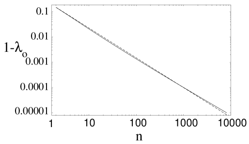
FIG. 4.: Optimal $\lambda$ as a function of $n$. The vertical axis shows $1-\lambda_{0}$ on a logarithmic scale. The horizontal axis plots $n$ on a logarithmic scale. The solid line is the numerical solution of Eq. (48) and the dashed line is the approximation given by Eq. (50).

For large $n$, using Eq. (50) we can approximate the optimal mutation rate by:

$$q_{o}=\frac{1}{3(nK)n^{0.175}}~{}.$$ (51)

Thus, the optimal mutation rate drops as a power-law in both $n$ and $K$. This implies that, generally for the Royal Staircase fitness function, the mutation rate should decrease as a GA run progresses so that the search will find the global optimum as quickly as possible. We pursue this idea more precisely elsewhere by considering an adaptive mutation rate scheme for the GA.

X Fitness Function Evaluations: Theory versus Experiment

In the preceding sections we derived an expression for the probability $C_{n+1}^{\prime}$ to create, over one generation in epoch $n$, a string of fitness $n+1$ that will stabilize by spreading through the population. From this we now estimate the total number $E$ of fitness function evaluations the GA uses on average before an optimal string of fitness $N+1$ is found. As a first approximation, we assume that the GA visits all epochs, that the time spent in innovations between them is negligible, and that epochs are always stable. By epoch stability we mean it is highly unlikely that strings with the current highest fitness will disappear from the population through a fluctuation, once such strings begin to spread. These assumptions appear to hold for the parameters of Figs. 3(a) and 3(c). They may hold even for the parameters of Fig. 3(b), but they probably do not for Fig. 3(d). For the parameters of Fig. 3(d), we see that the later epochs ($n=8$, $9$, and $10$) easily destabilize a number of times before the global optimum is found. We will develop a generalization that addresses this more complicated behavior in Ref. [35].

The average number $T_{n}$ of generations that the population spends in epoch $n$ is simply $1/C_{n+1}^{\prime}$, the inverse of the probability that a string of fitness $n+1$ will be discovered and spread through the population. For a population of size $M$, the number of fitness function evaluations per generation is $M$, so that the total number $E_{n}$ of fitness function evaluations in epoch $n$ is given by $T_{n}M$. More explicitly, we have from this and Eqs. (39) and (47) that:

$$E_{n}=\frac{2^{K}-1}{(1-\lambda)P^{n}_{n}\pi_{n}}~{}.$$ (52)

This says that, given our approximations, the total number of fitness function evaluations in each epoch is independent of the population size $M$. The epoch lengths, measured in generations, are inversely proportional to $M$, while the number of fitness function evaluations per generation is $M$. Substituting our analytical expressions for $P^{n}_{n}$ and $\pi_{n}$, Eqs. (33) and (46), we have:

$$E_{n}(\lambda)=\frac{2^{K}-1}{(1-\lambda)\left(1-e^{-2\left(1+\frac{1}{n}\right)\lambda+2}\right)}\prod_{i=1}^{n-1}\frac{n\lambda^{n-i-1}-i}{n\lambda^{n-i}-i}~{}.$$ (53)

In Ref. [35] we use this to derive analytical scaling expressions for the minimal number of function evaluations that the GA requires on average in epoch $n$ as given by $E_{n}(\lambda_{o})$, where $\lambda_{o}$ is the optimal $\lambda$ for epoch $n$.

The total number of fitness function evaluations $E(\lambda)$ to reach the global optimum is given by the sum of $E_{n}(\lambda)$ over all epochs $n$ from $1$ to $N$:

$$E(\lambda)=\sum_{n=1}^{N}\frac{2^{K}-1}{(1-\lambda)\pi_{n}(\lambda)}\prod_{i=1}^{n-1}\frac{n\lambda^{n-i-1}-i}{n\lambda^{n-i}-i}~{}.$$ (54)

The optimal mutation rate for an entire run is obtained by minimizing the above expression for $E$ with respect to $\lambda$.

Figure 5 compares Eq. (54) to the number (solid lines) of function evaluations estimated from 250 GA runs for the four different settings of $N$ and $K$ of Fig. 3. Each plot is a function of mutation rate $q$ and is given for a set of different population sizes $M$.

FIG. 5.: Comparison of experimental results (solid lines) and theoretical predictions (dashed lines) of the total number $E$ of function evaluations to reach the global optimal as a function of the mutation rate $q$, for four different fitness functions as determined by $N$ and $K$. The parameters are the same as those used in Fig. 3. Plot (a) has $N=8$ and $K=8$, (b) has $N=6$ and $K=6$, (c) has $N=4$ and $K=10$, and (d) has $N=10$ and $K=5$. The dashed lines give the theoretical predictions according to Eq. (54). The solid lines are the results of experiments with different population sizes $M$. Each data point on the solid lines gives $E$ averaged over $R=250$ GA runs. Each solid line shows the estimated $E$ as a function of $q$ for a constant population size $M$. For low mutation rates, the solid lines approximately overlap, indicating that $E$ is approximately independent of $M$ in this regime. For large mutation rates, the lower values of $M$ have larger $E$ than for larger $M$. Plot (a) shows, from left to right, population sizes $M=150$, $M=200$, $M=250$, $M=300$, and $M=350$; plot (b) $M=60$, $M=90$, $M=120$, $M=150$, $M=180$, and $M=210$; plot (c) $M=50$, $M=80$, $M=110$, $M=140$, $M=170$, and $M=200$; and finally, plot (d) $M=100$, $M=150$, $M=200$, $M=250$, and $M=300$.

Each of the four plots in Fig. 5 shows, as a dashed line, the population-size independent theoretical approximation of the total number $E$ of fitness function evaluations as a function of $q$. The four parameter settings of $N$ and $K$ are the same as in the runs (a), (b), (c), and (d) of Fig. 3. In each plot in Fig. 5 the solid lines show $E$ as a function of $q$ for several different population sizes as obtained from GA experiments. Each data point on the solid lines is an average over $250$ GA runs.

Figure 5(a) has $N=8$ blocks of $K=8$ bits. The dependence of $E$ on mutation rate is shown over the range from $q=0.001$ to $q=0.012$. The optimal mutation rate occurs somewhere around $q_{o}=0.006$. Each solid line shows the experimental dependence of $E$ on $q$ for a fixed population size. At high mutation rates, the lower population sizes have higher $E$. At high mutation rates, the set of solid lines in Fig. 5 show, from left to right, $E(q)$ for population sizes $M=150$, $M=200$, $M=250$, $M=300$, and $M=350$, respectively.

Figure 5(b) has parameters $N=6$ and $K=6$. $E(q)$ is shown over the range $q=0.001$ to $q=0.025$. Again, at large mutation rates the smaller population sizes have higher $E(q)$. The solid lines from top to bottom in the high mutation rate regime show $E(q)$ for population sizes $M=60$, $M=90$, $M=120$, $M=150$, $M=180$, and $M=210$, respectively. The optimal mutation rate occurs somewhere around $q_{o}=0.012$.

Figure 5(c) has $N=4$ blocks of length $K=10$ as parameter settings. $E(q)$ is shown over the range $q=0.001$ to $q=0.02$, the optimum occurring around $q_{o}=0.011$. The solid lines shows the experimental $E(q)$ for population sizes $M=50$, $M=80$, $M=110$, $M=140$, and $M=200$.

Finally, Fig. 5(d) has $N=10$ blocks of length $K=5$ bits. The horizontal axis ranges from $q=0.001$ to $q=0.016$ with the optimal mutation rate occurring around $q_{o}=0.008$. The population sizes are, from top to bottom at high $q$, $M=100$, $M=150$, $M=200$, $M=250$, and $M=300$, respectively. Note that for figures 5(b), 5(c), and 5(d) the tick marks on the vertical axis have a scale of $10^{5}$ fitness function evaluations, while Fig. 5(a) uses a scale of $10^{6}$ fitness function evaluations.

Note that in obtaining the theoretical predictions we have set $\pi_{N}=1$ in Eq. (54), since by definition the GA stops at the first occurrence of the globally optimum string. For the last epoch $N$ it is only necessary to create a string of fitness $N+1$, it does not need to spread through the population.

Figure 5 shows that for all these different parameter settings, the theory, which is independent of population size $M$, reasonably predicts the location of the optimal mutation rate $q_{o}$. It also predicts moderately well the shape of the curve around the optimum.

It is notable that the theory consistently underestimates $E(q)$. Furthermore, it underestimates $E(q)$ more in the low mutation rate regime than in the high. We believe that both of these offsets can be explained by the effects of finite-population sampling. We assumed that all unaligned blocks in members of the current highest fitness class are random and independent of each other. This last assumption does not hold in general [10]. Due to finite-population sampling and the resulting tendency to fixate, strings in the highest fitness class are correlated with each other. This means that if one individual in the highest fitness class has it’s $n$th unaligned block at a large Hamming distance from the desired configuration (with that block aligned), then many individuals (as descendants) in the highest fitness class also tend to have their $n$th blocks at large Hamming distances from the desired configuration. This genetic correlation among the individuals increases the epoch durations. Moreover, this effect is more severe for small mutation rates which, along with small population sizes, increase population convergence.

It turns out that this effect is difficult to analyze quantitatively. In spite of this it appears that, for low mutation rates on up to the optimal mutation rate, the total number $E$ of fitness function evaluations is indeed approximately independent of population size $M$. Moreover, the theory still accurately predicts the location of the optimal mutation rate $q_{o}$. Also, although the exact magnitude of $E$ is underestimated, the largest deviation in $E$ from the experimental minimum is $47$% for the parameters of Fig. 5(a), whereas the minimal deviation is $37$%, for the parameters of Fig. 5(c). Thus, the theory predicts the correct order of magnitude for the minimal number of fitness function evaluations.

As was noted above, the experimental curves for different population sizes appear to collapse onto each other in the low mutation rate regime. As the mutation rate increases, the solid curves break off this common curve one by one and do so delayed in proportion to population size. As the mutation rate increases it appears that progressively larger population sizes are necessary to maintain the search’s efficiency. Of course, this effect is not explained by our population-size independent theory. It is the topic of the sequel [35].

From the point of view of GA practice, it is important to emphasize again that there is a large variance between GA runs (at fixed parameters) in the total number of function evaluations to reach the global optimum. For example, if there is an average number of $10^{5}$ fitness function evaluations, then the standard deviation of the total number of fitness function evaluations is also almost $10^{5}$. Some runs may take as much as $5\times 10^{5}$ fitness function evaluations (say) and some may only take $10^{4}$ evaluations. Therefore, if one intends to use a GA for only a few runs, or maybe even just once, there is a large range of $q$ and $M$ for which the performance of the GA looks statistically identical. In other words, the GA has a large “sweet spot” with respect to parameter settings for optimal search. Note that the optimal mutation rate is generally well below $q=1/L$. Thus, despite the large parameter sweet spot, a mutation rate of $q=1/L$ is far too large for epochal evolutionary search.

XI Conclusion and Future Analyses

In summary our findings are the following.

1. At fixed population size $M$, there is a smooth cost surface $E(q)$ as a function of mutation rate $q$. It has a single and shallow minimum $q_{o}$.

2. The optimal mutation rate $q_{o}$ roughly occurs in the regime where the highest epochs $N-1$, $N$, and $N+1$ are marginally stable; see Fig. 3.

3. For lower mutation rates than $q_{o}$ the total number of fitness function evaluations $E(q)$ grows steadily and becomes almost independent of the population size $M$.

4. Crossover’s role in reducing search time is marginal due to population convergence during the epochs.

5. There is an mutational error threshold in $q$ that bounds the upper limit of the GA’s efficient search regime. Above the threshold, which is population-size independent, suboptimal strings of fitness $N$ cannot stabilize in the population.

6. The surface $E(q)$ appears to be everywhere concave. That is, for any two parameters $q_{1}$ and $q_{2}$, the straight line connecting these two points is everywhere above the surface $E(q)$. We conjecture that this is always the case for mutation-only genetic algorithms with a static fitness function. This feature is useful in that a steepest-descent algorithm applied to parameter $q$ will lead to the unique optimum $q_{o}$.

Synopsizing the results this way, we are anticipating some of the results developed for the population-size dependent theory [35].

In this sequel we extend the above statistical dynamics analysis to account for $E(q)$’s dependence on population size. This not only improves the parameter-optimization theory, but also leads us to consider a number of issues and mechanisms that shed additional light on how GAs work and on those types of search problems (fitness functions) for which evolutionary search is and is not well suited. Since it appears that optimal parameter settings often lead the GA to run in a mode were the population dynamics is marginally stable in the higher epochs, we consider how epoch destabilization affects epoch stability and duration. We also analyze an adaptive evolutionary search algorithm in which the mutation rate and population size change dynamically as successive epochs are encountered. This leads to a reduction in search time and in resource requirements.

REFERENCES

- [1] C. Adami. Self-organized criticality in living systems. Phys. Lett. A, 203:29–32, 1995.
- [2] T. Back. Evolutionary algorithms in theory and practice: Evolution strategies, evolutionary programming, genetic algorithms. Oxford University Press, New York, 1996.
- [3] L. Barnett. Tangled webs: Evolutionary dynamics on fitness landscapes with neutrality. Master’s thesis, School of Cognitive Sciences, University of East Sussex, Brighton, 1997. http://www.cogs.susx.ac.uk/ lab/adapt/nnbib.html.
- [4] R. K. Belew and L. B. Booker, editors. Proceedings of the Fourth International Conference on Genetic Algorithms. Morgan Kaufmann, San Mateo, CA, 1991.
- [5] A. Bergman and M. W. Feldman. Question marks about the period of punctuation. Technical report, Santa Fe Institute Working paper 96-02-006, 1996.
- [6] L. Chambers, editor. Practical handbook of genetic algorithms, Boca Raton, 1995. CRC Press.
- [7] J. P. Crutchfield. Subbasins, portals, and mazes: Transients in high dimensions. J. Nucl. Phys. B, 5A:287, 1988.
- [8] J. P. Crutchfield and M. Mitchell. The evolution of emergent computation. Proc. Natl. Acad. Sci. U.S.A., 92:100742–10746, 1995.
- [9] L. D. Davis, editor. The Handbook of Genetic Algorithms. Van Nostrand Reinhold, 1991.
- [10] B. Derrida and L. Peliti. Evolution in a flat fitness landscape. Bull. Math. Bio., 53(3):355–382, 1991.
- [11] M. Eigen. Self-organization of matter and the evolution of biological macromolecules. Naturwissen., 58:465–523, 1971.
- [12] M. Eigen and P. Schuster. The hypercycle. A principle of natural self-organization. Part A: Emergence of the hypercycle. Naturwissen., 64:541–565, 1977.
- [13] S. F. Elena, V. S. Cooper, and R. E. Lenski. Punctuated evolution caused by selection of rare beneficial mutations. Science, 272:1802–1804, 1996.
- [14] L. Eshelman, editor. Proceedings of the Sixth International Conference on Genetic Algorithms. Morgan Kaufmann, San Mateo, CA, 1995.
- [15] W. Fontana and P. Schuster. Continuity in evolution: On the nature of transitions. Science, 280:1451–5, 1998.
- [16] W. Fontana, P. F. Stadler, E. G. Bornberg-Bauer, T. Griesmacher, et al. RNA folding and combinatory landscapes. Phys. Rev. E, 47:2083–99, 1992.
- [17] S. Forrest, editor. Proceedings of the Fifth International Conference on Genetic Algorithms. Morgan Kaufmann, San Mateo, CA, 1993.
- [18] C. V. Forst, C. Reidys, and J. Weber. Evolutionary dynamics and optimizations: Neutral networks as model landscapes for RNA secondary-structure folding landscape. In F. Moran, A. Moreno, J. Merelo, and P. Chacon, editors, Advances in Artificial Life, volume 929 of Lecture Notes in Artificial Intelligence. Springer, 1995. SFI preprint 95-20-094.
- [19] S. J. Gould and N. Eldredge. Punctuated equilibria: The tempo and mode of evolution reconsidered. Paleobiology, 3:115–251, 1977.
- [20] R. Haygood. The structure of Royal Road fitness epochs. Evolutionary Computation, submitted, ftp://ftp.itd.ucdavis.edu/pub/people/rch/ StrucRoyRdFitEp.ps.gz, 1997.
- [21] J. H. Holland. Adaptation in Natural and Artificial Systems. MIT Press, Cambridge, MA, 1992. Second edition (First edition, 1975).
- [22] M. Huynen. Exploring phenotype space through neutral evolution. Technical Report 95-10-100, Santa Fe Institute, Santa Fe, NM, USA, October 1995.
- [23] M. Huynen, P. F. Stadler, and W. Fontana. Smoothness within ruggedness: The role of neutrality in adaptation. Proc. Natl. Acad. Sci., 93:397–401, 1996.
- [24] S. A. Kauffman and S. Levin. Towards a general theory of adaptive walks in rugged fitness landscapes. J. Theo. Bio., 128:11–45, 1987.
- [25] M. Kimura. The neutral theory of molecular evolution. Cambridge University Press, 1983.
- [26] J. R. Koza. Genetic programming: On the programming of computers by means of natural selection. MIT Press, Cambridge, MA, 1992.
- [27] C. A. Macken and A. S. Perelson. Protein evolution in rugged fitness landscapes. Proc. Nat. Acad. Sci., 86:6191–6195, 1989.
- [28] M. Mitchell, J. P. Crutchfield, and P. T. Hraber. Evolving cellular automata to perform computations: Mechanisms and impediments. Physica D, 75:361–391, 1994.
- [29] M. Newman and R. Engelhardt. Effect of neutral selection on the evolution of molecular species. Proc. R. Soc. London B., in press, 1998. SFI preprint 98-01-001.
- [30] A. E. Nix and M. D. Vose. Modeling genetic algorithms with Markov chains. Ann. Math. Art. Intel., 5, 1991.
- [31] A. Prug̈el-Bennett and J. L. Shapiro. Analysis of genetic algorithms using statistical mechanics. Phys. Rev. Lett., 72(9):1305–1309, 1994.
- [32] A. Prügel-Bennett and J. L. Shapiro. The dynamics of a genetic algorithm in simple random Ising systems. Physica D, 104 (1):75–114, 1997.
- [33] M. Rattray and J. L. Shapiro. The dynamics of a genetic algorithm for a simple learning problem. J. of Phys. A, 29(23):7451–7473, 1996.
- [34] C. M. Reidys, C. V. Forst, and P. K. Schuster. Replication and mutation on neutral networks of RNA secondary structures. Bull. Math. Biol., 59(2), 1998.
- [35] E. van Nimwegen and J. P. Crutchfield. Optimizing epochal evolutionary search: Population-size dependent theory. Machine Learning, 1998. submitted. Santa Fe Institute Working Paper 98-10-090.
- [36] E. van Nimwegen, J. P. Crutchfield, and M. Mitchell. Finite populations induce metastability in evolutionary search. Phys. Lett. A, 229:144–150, 1997.
- [37] E. van Nimwegen, J. P. Crutchfield, and M. Mitchell. Statistical dynamics of the Royal Road genetic algorithm. Theoretical Computer Science, special issue on Evolutionary Computation, A. Eiben, G. Rudolph, editors, in press, 1998. SFI working paper 97-04-35.
- [38] M. D. Vose. Generalizing the notion of schema in genetic algorithms. Artificial Intelligence, 50:385–396, 1991.
- [39] M. D. Vose and G. E. Liepins. Punctuated equilibria in genetic search. Complex Systems, 5:31–44, 1991.
- [40] J. Weber. Dynamics of Neutral Evolution. A case study on RNA secondary structures. PhD thesis, Biologisch-Pharmazeutischen Fakultät der Friedrich Schiller-Universität Jena, 1996.
- [41] D. Wolpert and W. Macready. No free lunch theorems for search. Technical Report SFI-TR-95-02-010, Santa Fe Institute, Santa Fe, NM, USA, February 1995.
- [42] S. Wright. Character change, speciation, and the higher taxa. Evolution, 36:427–43, 1982.