Coupling Impedances of Azimuthally Symmetric Obstacles
of Semi-Elliptical Shape in a Beam Pipe

Abstract

The beam coupling impedances of small axisymmetric obstacles having a semi-elliptical cross section along the beam in the vacuum chamber of an accelerator are calculated at frequencies for which the wavelength is large compared to a typical size of the obstacle. Analytical results are obtained for both the irises and the cavities with such a shape which allow simple estimates of their broad-band impedances.

I Introduction

High currents in modern accelerators and colliders severely restrict the allowed coupling impedance of the machine. For this reason, it is important to know the impedance contributions even from small discontinuities of the vacuum chamber.

In a recent paper [1], Kurennoy has analytically calculated the low-frequency coupling impedance of small obstacles protruding into a beam pipe. In this paper we present an alternative derivation for an azimuthally symmetric semi-elliptical object protruding into a beam pipe, which confirms the dependence on the depth, but not on the width, of the protrusion. We also study the more difficult — from the analytical point of view — case of an axisymmetric semi-elliptical protrusion outside the beam pipe (cavity), and present variational results for different elliptical eccentricities.

II General Analysis

Consider a beam pipe of radius $R_{\rm pipe}$ and an azimuthally symmetric obstacle whose dimensions are small compared with both $R_{\rm pipe}$ and $\lambda$, the rf wavelength. We start with the definition of the longitudinal impedance as [2]

$$Z_{\parallel}(k)=\frac{1}{|I_{0}|^{2}}\int dv\vec{E}\cdot J^{*},$$ (1)

where the current in the frequency domain for an ultrarelativistic point charge is

$$J_{z}(x,y,z;k)=I_{0}\delta(x)\delta(y)\exp(-jkz),$$ (2)

with $k=w/c=2\pi/\delta$, and with the implied time dependence of all quantities being $\exp(jwt)$. We then identify two configurations:  the subscript 1 denotes the pipe without the obstacle and the subscript 2 denotes the pipe with the obstacle. By forming the combination

$\displaystyle-\int dv(\mbox{\boldmath$E$}_{2}\cdot\mbox{\boldmath$J$}^{*}+\mbox{\boldmath$E$}_{1}^{*}\times\mbox{\boldmath$J$})$

and using Maxwell’s equations to write $J$ in terms of the fields $E$ and $H$, we write the contribution of the obstacle to the impedance as

$$|I_{0}|^{2}Z_{u}(k)=\int_{S_{2}\neq S_{1}}dS_{2}\mbox{\boldmath$n$}_{2}\cdot\mbox{\boldmath$E$}_{1}^{*}\times\mbox{\boldmath$H$}_{2},$$ (3)

where the surface integral is only over the surface of the obstacle. Using

$$E^{*}_{1r}=\frac{Z_{0}I_{0}^{*}}{2\pi r}\exp(jkz)$$ (4)

and

$$\mbox{\boldmath$n$}_{2}dS_{2}=2\pi r[\hat{\mbox{\boldmath$n$}}dz-\hat{\mbox{\boldmath$z$}}dr],$$ (5)

with $\hat{\mbox{\boldmath$r$}}$ and $\hat{\mbox{\boldmath$z$}}$ being unit vectors, we have

$$\frac{Z_{\parallel}(k)}{Z_{0}}=-\frac{1}{I_{0}}\int drH_{2\phi}e^{jkz}.$$ (6)

Figure 1 show the geometry for an obstacle protruding into and outside of the beam pipe.

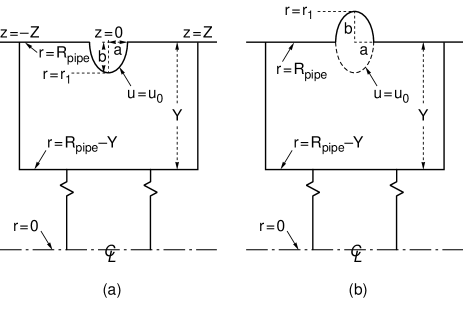
FIG. 1.: The beam pipe with an interior (a) and exterior (b) obstacle. One assumes $a,b\ll Y,Z\ll\lambda,R_{\rm pipe}$.

A more explicit form for Eq. (2.6) is

$$\frac{Z_{\parallel}(k)}{Z_{0}} = -\frac{1}{I_{0}}\left[\int^{r_{1}}_{R_{\rm pipe}}drH_{2\phi}(r,z_{a}(r))e^{jkz(r)}\right.$$ (7)

$$+ \left.\int^{R_{\rm pipe}}_{r_{1}}drH_{2\phi}(r,z_{b}(r))e^{jkz(r)}\right]$$ (8)

We now convert the bracket in Eq. (2.7) to a double integral for the obstacle in Fig. 1a:

$$[\ ] = \int^{R_{\rm pipe}}_{r_{1}}\int^{z_{a}(r)}_{-Z}dz\frac{\partial}{\partial z}(H_{2\phi}e^{jkz})$$ (9)

$$+ \left.\int^{R_{\rm pipe}}_{r_{1}}dr(H_{2\phi}e^{jkz})\right|_{z=-Z}$$ (10)

$$+ \int^{R_{\rm pipe}}_{r_{1}}dr\int^{Z}_{z_{b}(r)}dz\frac{\partial}{\partial z}(H_{2\phi}e^{jzk})$$ (11)

$$- \left.\int^{R_{\rm pipe}}_{r_{1}}dr(H_{2\phi}e^{jkz})\right|_{z=Z}.$$ (12)

Here $Z$ is a distance large compared with the dimensions of the obstacle, but small compared with $\lambda$ and $R_{\rm pipe}$, so that $H_{2\phi}\exp(jkz)$ takes on its value in a pipe without an obstacle at $z=\pm Z$, namely

$$H_{2\phi}(\pm Z)=I_{0}\exp(\mp jkZ).$$ (13)

This causes the 2nd and 4th terms on the right side of Eq. (2.8) to cancel. We also add the vanishing term

$$\int^{r_{1}}_{R_{\rm pipe}-Y}dr\int^{Z}_{-Z}dz\frac{\partial}{\partial z}(H_{2\phi}e^{jkz}),$$ (14)

and finally obtain

$$\frac{Z_{\parallel}(k)}{Z_{0}}=\frac{1}{I_{0}}\int\!\!\int_{\stackrel{{\scriptstyle\mbox{solid}}}{{\mbox{border}}}}drdz\frac{\partial}{\partial z}(H_{2\phi}e^{jkz}),$$ (15)

where the area of integration is within the solid border in Fig. 1a. Parallel arguments lead to the same result for the obstacle in Fig. 1b.

We now use Maxwell’s equations to rewrite Eq. (2.11) as

$$\frac{Z_{\parallel}(k)}{Z_{0}}=-\frac{jk}{Z_{0}I_{0}}\int\!\!\int_{\stackrel{{\scriptstyle\mbox{solid}}}{{\mbox{border}}}}drdz(E_{r}-Z_{0}H_{\phi})e^{jkz}$$ (16)

where we have dropped the subscript 2. For low frequency we set $\exp(jkz)=1$ and obtain

$$\frac{Z_{\parallel}(k)}{Z_{0}}\cong-\frac{jk}{Z_{0}I_{0}}\int\!\!\int_{\stackrel{{\scriptstyle\mbox{solid}}}{{\mbox{border}}}}drdz(E_{r}-Z_{0}H_{\phi}).$$ (17)

Clearly our derivation has resulted in a separation into a term involving the electric polarizability and a term involving the magnetic susceptibility (in the azimuthal direction) as in previous work [3, 4, 5, 6]. Since the obstacles are azimuthally symmetric, we can replace $Z_{0}H_{\phi}$ in the vicinity of the obstacle by

$$Z_{0}H_{\phi}=E_{0}=Z_{0}I_{0}/(2\pi R_{\rm pipe})$$ (18)

and find

$$\frac{Z_{\parallel}(k)}{Z_{0}}=\frac{jk}{2\pi R_{\rm pipe}}\int\!\!\int_{\stackrel{{\scriptstyle\mbox{solid}}}{{\mbox{border}}}}drdz\left(\frac{E_{r}-E_{0}}{E_{0}}\right).$$ (19)

III Semi-Elliptical Interior Obstacle — Iris

We now proceed to calculate Eq. (2.15) explicitly for the geometry of Fig. 1a. We change from the variable $r$ to the variable

$$y=R_{\rm pipe}-r,$$ (20)

with $|y|\ll\lambda$, $|y|\ll R_{\rm pipe}$, and we use elliptical coordinates [7] defined by

$$\left.\begin{array}[]{l}y=c\cosh u\cos v,\ \ z=c\sinh u\sin v\\ a=c\sinh u_{0}\ ,\ b=c\cosh u_{0},\ \ c^{2}=b^{2}-a^{2}\end{array}\right\}.$$ (21)

The metric (Jacobian) is defined by

$$dzdy=c^{2}D(u,v)dudv,$$ (22)

where

$$D(u,v)=\cosh^{2}u\sin^{2}v+\sinh^{2}u\cos^{2}v,$$ (23)

and the Laplacian operator can be written as

$$\frac{\partial^{2}}{\partial x^{2}}+\frac{\partial^{2}}{\partial y^{2}}=\frac{1}{c^{2}D(u,v)}\left(\frac{\partial^{2}}{\partial u^{2}}+\frac{\partial^{2}}{\partial v^{2}}\right).$$ (24)

The solution to Laplace’s equation for the electrostatic potential in the region $u\geq u_{0}$, with $\Psi(u_{0},v)=0$, and with the asymptotic field $E_{0}$, is

$$\Psi(u,v)=cE_{0}\cos v[\cosh u-e^{u_{0}-u}\cosh u_{0}]$$ (25)

where

$$E_{r} = -\frac{\partial\Psi}{\partial r}=\frac{\partial\Psi}{\partial y}$$ (26)

$$= E_{0}-cE_{0}e^{u_{0}}\cosh u_{0}\frac{\partial}{\partial y}(\cos ve^{-u}).$$ (27)

Here we choose $\cos v$ in the second term to preserve the symmetry around $v=0$ ($z=0$), and to satisfy the boundary condition for all $v$ at $u=u_{0}$ and for $v=\pm\pi/2$ with $u\geq u_{0}$. Also we have

$$\frac{\partial}{\partial y} = \frac{\partial u}{\partial y}\frac{\partial}{\partial u}+\frac{\partial v}{\partial y}\frac{\partial}{\partial v}$$ (28)

$$= \frac{1}{cD(u,v)}\left[\sinh u\cos v\frac{\partial}{\partial u}-\cosh u\sin v\frac{\partial}{\partial v}\right].$$ (29)

Applying this to Eq. (3.7) for $E_{r}-E_{0}$, we find from Eq. (3.6) that

$$\frac{Z_{\parallel}(k)}{Z_{0}}=\frac{-jkc^{2}}{2\pi R_{\rm pipe}}e^{u_{0}}\cosh u_{0}\times$$ (30)

$$\quad\int\!\!\int dudv\,[\cos^{2}ve^{-u}\sinh u-\sin^{2}ve^{-u}\cosh u]$$ (31)

$$=\frac{jkc^{2}e^{u_{0}}\cosh u_{0}}{2R_{\rm pipe}}\int\!\!\int_{\stackrel{{\scriptstyle\mbox{solid}}}{{\mbox{border}}}}dudv\,[e^{-2u}-\cos 2v],$$ (32)

where we have used Eq. (2.14).

We now let $Z\rightarrow\infty$ and cut off the integration over $v$ where

$$y = c\cosh u_{\rm max}\cos v=Y,\quad\mbox{ or}$$ (33)

$$u_{\rm max} = \cosh^{-1}\frac{Y}{c\cos v}\gg 1\ .$$ (34)

This leads to

$$\frac{Z_{\parallel}(k)}{Z_{0}} = \frac{jkc^{2}e^{u_{0}}\cosh u_{0}}{4\pi R_{\rm pipe}}\int^{\frac{\pi}{2}}_{-\frac{\pi}{2}}dv\int^{u_{\rm max}}_{u_{0}}du[e^{-2u}-\cos v]$$ (35)

$$\cong \frac{jkc^{2}e^{u_{0}}\cosh u_{0}}{4\pi R_{\rm pipe}}\left[\vphantom{\int^{\frac{\pi}{2}}_{-\frac{\pi}{2}}}\frac{\pi}{2}e^{-2u_{0}}\right.$$ (36)

$$- \left.\int^{\frac{\pi}{2}}_{-\frac{\pi}{2}}dv\cos 2v\left(\ln\frac{2Y}{c\cos v}-u_{0}\right)\right],$$ (37)

or

$$\frac{Z_{\parallel}(k)}{Z_{0}}=\frac{jkc^{2}\cosh^{2}u_{0}}{4R_{\rm pipe}}=\frac{jkb^{2}}{4R_{\rm pipe}}$$ (38)

where the last integral in (3.11) was done by parts for $Y\gg c$.

For $a>b$ we need to modify our elliptical coordinates so that

$$\left.\begin{array}[]{l}y=c\sinh u\sin v,\ \ z=c\cosh u\cos v\\ a=c\cosh u_{0}\ ,\ b=c\sinh u_{0},\ \ c^{2}=a^{2}-b^{2}\end{array}\right\}.$$ (39)

The matrix is unchanged, but now

$$\frac{\partial}{\partial y}=\frac{1}{D(u,v)}\left[\frac{\cosh u\sin v}{c}\frac{\partial}{\partial u}+\frac{\sinh u\cos v}{c}\frac{\partial}{\partial v}\right].$$ (40)

This time one finds

$$\frac{Z_{\parallel}(k)}{Z_{0}}=\frac{jkc^{2}\sinh^{2}u_{0}}{4R_{\rm pipe}}=\frac{jkb^{2}}{4R_{\rm pipe}},$$ (41)

that is the result is unchanged from Eq. (3.12), again depending only on the depth of the elliptical protrusion into the pipe and not on its width, as also found by Kurennoy [1].

IV Semi-Elliptical Exterior Obstacle — Cavity

A Analytical Approach

We now turn to the exterior semi-elliptical obstacle in Fig. 1b. Here we need to choose appropriate potential forms for $u\leq u_{0}$, and for $u\geq u_{0}$, and match them at $u=u_{0}$.

We again start with Eq. (2.15) and work with the complete set of solutions of the Laplace equation, namely $\cos nv\exp(\pm nu)$ and $\sin nv\exp(\pm nu)$. For $u\geq u_{0}$, (and $b>a$) with the asymptotic field $E_{0}$, we choose

$$\Psi(u,v)=E_{0}y-cE_{0}\sum^{\infty}_{n=1}\alpha_{n}\cos nve^{-nu}$$ (42)

in order to satisfy the even symmetry about $v=0$ ($z=0$) and $\Psi(u,\pm\pi/2)=0$ for $u\geq u_{0}$. If we write

$$\Psi(u_{0},v)=cE_{0}f(v),$$ (43)

where $f(v)$ is, as yet, an unknown function, we can solve for $\alpha_{n}$ in terms of $f(v)$ to obtain

$$\alpha_{n}=-\frac{2}{\pi}e^{nu_{0}}f_{n}+e^{u_{0}}\cosh u_{0}\delta_{n1},$$ (44)

where

$$f_{n}\equiv\int^{\frac{\pi}{2}}_{-\frac{\pi}{2}}dv\cos nvf(v).$$ (45)

For $u\leq u_{0}$, we write

$$\Psi(u,v)=\sum^{\infty}_{m=1}\beta_{n}\cos nv\cosh mu$$ (46)

for a potential which is well behaved within the ellipse. Recognizing in this case that $f(v)=0$ for $\pi/2<|v|<\pi$, we solve for $\beta_{m}$ in terms of $f(v)$ to obtain

$$\beta_{m}=\frac{f_{m}}{\pi\cosh mu_{0}},$$ (47)

where $f_{m}$ is consistent with the definition in Eq. (4.4). Both odd and even values of $m$ must be included.

We now calculate the impedance as we did in the previous section, this time including the regions $u\geq u_{0}$, $|v|\leq\pi/2$ and $u\leq u_{0}$, $|v|\leq\pi$. For $u\geq u_{0}$ we find

$$\frac{Z_{\parallel}^{(>)}(k)}{Z_{0}}\ =\ -\frac{jkc^{2}}{4\pi R_{\rm pipe}}\int\!\!\int_{\stackrel{{\scriptstyle{u\geq u_{0}}}}{{{y<Y}}}}dudv\sum^{\infty}_{\stackrel{{\scriptstyle{n=1}}}{{\mbox{odd}}}}n\alpha_{n}\,\times$$ (48)

$$\ \left[e^{-(n-1)u}\cos(n+1)v-e^{-(n+1)u}\cos(n-1)v\right].$$ (49)

Clearly, only the terms with $n=1$ survive, leading ultimately to

$$\frac{Z_{\parallel}^{(>)}(k)}{Z_{0}}=\frac{jkc^{2}}{4R_{\rm pipe}}\alpha_{1}e^{-u_{0}}\cosh u\ .$$ (50)

For $u\leq u_{0}$ we separate the two terms in Eq. (2.15). The second is simply

$$\frac{Z_{\parallel,2}^{(<)}(k)}{Z_{0}}=\frac{jkab}{\pi 4R_{\rm pipe}}=\frac{jkc^{2}\cosh u_{0}\sinh u_{0}}{4R_{\rm pipe}}$$ (51)

The first is

$$\frac{Z_{\parallel,1}^{(<)}(k)}{Z_{0}}=-\frac{jkc^{2}}{4\pi R_{\rm pipe}}\int\!\!\int_{u\leq u_{0}}dudv$$ (52)

$$\ \times\sum^{\infty}_{m=1}m\beta_{m}[\cosh(m+1)u\cos(m-1)v$$ (53)

$$\qquad+\cosh(m-1)u\cos(m+1)v].$$ (54)

Again, only the term $m=1$ survives, and is

$$\frac{Z_{\parallel,1}^{(<)}(k)}{Z_{0}}=-\frac{jkc^{2}}{4R_{\rm pipe}}\beta_{1}\cosh u_{0}\sinh u_{0}.$$ (55)

Using Eqs. (4.3) and (4.6) we have for the impedance

$$\frac{Z_{\parallel}(k)}{Z_{0}}=\frac{jk}{2R_{\rm pipe}}\left[\frac{b^{2}}{2}+ab-(a+b)^{2}\frac{f_{1}}{\pi}e^{-u_{0}}\right].$$ (56)

In order to find $f_{1}$, we must obtain and solve the integral equation which represents the match of $\partial\Psi/\partial u$ at $u=u_{0}$, $|v|\leq\pi/2$. Here

$$\left.\frac{\partial\Psi}{\partial u}\right|_{u=u_{o^{+}}} = cE_{0}\left[\vphantom{\sum^{\infty}_{\stackrel{{\scriptstyle n=1}}{{\rm odd}}}}\sinh u_{0}\cos v\right.$$ (57)

$$+ \left.\sum^{\infty}_{\stackrel{{\scriptstyle{n=1}}}{{\mbox{odd}}}}n\alpha_{n}e^{-nu_{0}}\cosh v\right]$$ (58)

and

$$\left.\frac{\partial\Psi}{\partial u}\right|_{u=u_{o^{-}}}=cE_{0}\sum^{\infty}_{m=1}m\beta_{m}\sinh mu_{0}\cos mv.$$ (59)

Equating Eqs. (4.13) and (4.14), and using Eqs. (4.3) and (4.6), we find

$$\int^{\frac{\pi}{2}}_{-\frac{\pi}{2}}dv^{\prime}f(v^{\prime})K(v,v^{\prime})=\pi\cos ve^{u_{0}}$$ (60)

where

$$K(v,v^{\prime}) = \sum^{\infty}_{\stackrel{{\scriptstyle{n=1}}}{{\mbox{odd}}}}(2+\tanh nu_{0})\,n\cos nv\cos uv^{\prime}$$ (61)

$$+ \sum^{\infty}_{\stackrel{{\scriptstyle{m=2}}}{{\mbox{even}}}}m\tanh mu_{0}\cos mv\cos mv.$$ (62)

We now multiply Eq. (4.15) by $\int^{\frac{\pi}{2}}_{-\frac{\pi}{2}}dvf(v)$ to obtain

$$\frac{\left[\int^{\frac{\pi}{2}}_{-\frac{\pi}{2}}dvf(v)\cos v\right]^{2}}{\int^{\frac{\pi}{2}}_{-\frac{\pi}{2}}dvf(v)\int^{\frac{\pi}{2}}_{-\frac{\pi}{2}}dv^{\prime}f(v^{\prime})K(v,v^{\prime})} = \frac{\int^{\frac{\pi}{2}}_{-\frac{\pi}{2}}dvf(v)\cos v}{\pi e^{u_{0}}}$$ (63)

$$= \frac{f_{1}e^{-u_{0}}}{\pi}.$$ (64)

This is a variational form for $f_{1}$, the only unknown parameter in Eq. (4.12) for the impedance. An accurate numerical value for $Z_{\parallel}(k)/Z_{0}$ can be found by expanding $f(v)$ into a complete set in the interval $|v|\leq\pi/2$, then truncating and solving the resulting matrix equations obtained by maximizing Eq. (4.17). We write

$$f(v)=\sum^{P}_{\stackrel{{\scriptstyle{p=1}}}{{\mbox{odd}}}}c_{p}\sin\left(p\frac{\pi}{2}\right)\frac{\cos pv}{p},$$ (65)

truncated at $p=P$ and normalize $f(v)$ so that $c_{1}=1$. This leads to

$$\frac{f_{1}e^{-u_{o}}}{\pi}=\left[\vphantom{\sum^{P}_{\stackrel{{\scriptstyle p=3}}{{\rm odd}}}}H_{11}\right. + 2\sum^{P}_{\stackrel{{\scriptstyle{p=3}}}{{\mbox{odd}}}}c_{p}H_{p1}$$ (66)

$$+ \left.\sum^{P}_{\stackrel{{\scriptstyle{p=3}}}{{\mbox{odd}}}}\sum^{P}_{\stackrel{{\scriptstyle{q=3}}}{{\mbox{odd}}}}c_{p}c_{q}H_{pq}\right]^{-1},$$ (67)

where the symmetric matrix $H_{pq}$ is

$$H_{pq}=H_{qp} = \frac{2+\tanh pu_{0}}{P}\delta_{pq}$$ (68)

$$+ \frac{16}{\pi^{2}}\sum^{\infty}_{\stackrel{{\scriptstyle m=2}}{{\mbox{even}}}}\frac{m\tanh mu_{0}}{(m^{2}-p^{2})(m^{2}-q^{2})}.$$ (69)

Maximizing Eq. (4.19) with respect to the coefficients $c_{p}$, $p=3,5,\cdots,P$, leads to

$$\frac{f_{1}e^{-u_{o}}}{\pi}=\left[H_{11}-\sum^{P}_{\stackrel{{\scriptstyle{p=3}}}{{\mbox{odd}}}}\sum^{P}_{\stackrel{{\scriptstyle{q=3}}}{{\mbox{odd}}}}H_{1p}(H^{-1})_{pq}H_{q1}\right]^{-1}.$$ (70)

Here $(H^{-1})_{pq}$ is the inverse of the matrix $H_{pq}$ with $p$ and $q=3,5,7\cdots P$. This square matrix has the dimension

$$(P-1)/2\ {\rm by}\ (P-1)/2.$$ (71)

Note that

$$\tanh pu_{0}=\left(1-w^{p}\right)/\left(1+w^{p}\right)$$ (72)

and

$$\tanh mu_{0}=\left(1-w^{m}\right)/\left(1+w^{m}\right)$$ (73)

with

$$w=(b-a)/(b+a)\ .$$ (74)

The final result for the impedance is given in Eq. (4.12), using Eqs. (4.20) and (4.21).

The analysis for an obstacle with $a>b$ proceeds in a similar, but not identical pattern. The result is once again Eq. (4.12), using Eqs. (4.20) and (4.21), with only one change in Eq. (4.20):

$\displaystyle\tanh pu_{0}\rightarrow\coth pu_{0},$

with $\tanh u_{0}$ now being $a/b$ instead of $b/a$. Thus $w$ in Eq. (4.25) is replaced by $-w$ in Eq. (4.23), but the use of $\coth pu_{0}$ instead of $\tanh pu_{0}$ for odd $p$ leaves the expression for $H_{pq}$ in terms of $a$ and $b$ unchanged. The same is true for the term $\tanh mu_{0}$ in Eq. (4.24) since $m$ is even. So the final expression in Eq. (4.12) is unchanged provided $H_{pq}$ in Eqs. (4.20) and (4.21) is expressed in terms of $a$ and $b$.

B Variational Approach - Numerical Results

We proceed with a numerical investigation of the variational scheme described by Eqs. (4.12)-(4.21). Truncating the sum in the denominator of Eq. (4.21) at different $N=(P-1)/2=1,2,3,\ldots$, we explore the scheme convergence, and compare the results for the impedance (4.12) with those obtained by other methods. In doing so, it is convenient to rewrite Eq. (4.12) in the following form

$$\frac{Z_{\|}(k)}{Z_{0}}=\frac{jk}{2\pi R_{\rm pipe}}\frac{\pi ab}{2}F\left(\frac{a}{b}\right),$$ (75)

where

$$F(x)=\frac{1}{x}+2-\frac{2(1/x+2+x)}{2+x+16s(x)/\pi^{2}-\Sigma(x)},$$ (76)

and

$$s(x)=\frac{1}{8}\sum_{n=1}^{\infty}\frac{n}{(n^{2}-1/4)^{2}}\frac{(1+x)^{2n}-(1-x)^{2n}}{(1+x)^{2n}+(1-x)^{2n}}.$$ (77)

Here $\Sigma(x)$ denotes the sum in the denominator of Eq. (4.21) which is to be truncated.

The advantage of the representation (4.26) is that we know the asymptotic behavior of $F(x)$ for two limiting cases. For $x\ll 1$, i.e., when $a\ll b$, but still $b\ll R_{\rm pipe}$ — a short and deep enlargement — it has been demonstrated in [8] that

$$F(x)\to 1-\frac{4}{\pi^{2}}x.$$ (78)

In this limit, the inductive impedance in Eq. (4.26) is mostly of magnetic origin: the beam magnetic field fills the cavity volume without being substantially perturbed, and therefore the inductance is simply proportional to the area of the obstacle cross section. A correction of the order of $x=a/b$ to this term comes from the electric contribution. For a deep pillbox of depth $h$ which is much larger than width $g$, the electric contribution was calculated in [8] by means of conformal mapping. It results in the electric term $-g^{2}/(2\pi)$, which is small compared to the magnetic one, equal to $hg$ for such a pillbox. Obviously, the shape of a short and deep enlargement — rectangular or semi-elliptical — does not affect the electric term as long as $g\ll h$, since the beam electric field does not penetrate deeply into such a cavity, unlike the magnetic one. Substituting $g=2a$ into the electric term, and replacing the pillbox area $hg$ by the semi-ellipse area $\pi ab/2$ leads to the asymptotic form in Eq. (4.29).

The opposite limit, $x\gg 1$, corresponds to a very shallow cavity, $a\ll b$. It has been shown for many particular shapes of such cavities (see [8] and references therein) that the low-frequency impedance of a small shallow cavity of the depth $h$ and of an iris with the same cross section and having the same depth, are both inductive, equal to each other, and in the leading order are proportional to $h^{2}$. Since we already know the answer for a semi-elliptical iris (see Section III) we expect that for $x\gg 1$

$$F(x)\to\frac{1}{x},$$ (79)

to match the low-frequency impedance of the shallow iris, given in Eq. (3.15).

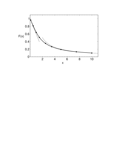
FIG. 2.: Function $F(x)$ versus ellipse aspect ratio $x=a/b$. The solid curve is an interpolation of numerical results (thick points). The dashed lines show the asymptotic behavior Eqs. (4.29) and (4.30).

The results of our numerical study are shown in Fig. 2, where the function $F(x)$ is plotted against the ellipse aspect ratio $x=a/b$. The convergence of the variational scheme is rather fast for all values of $x$; in fact, results obtained with $N=1$ (i.e., when the matrix in the sum $\Sigma(x)$ is truncated to merely a single number) and those for $N=8$, when the matrix has size $8\times 8$, differ by less than 0.5%. And, of course, we can obtain the asymptotic value of $F(x)$ for large $N$ with much better accuracy, well below $10^{-3}$, simply by extrapolating the results for different matrix sizes at fixed $x$. Figure 2 also shows very good agreement with the expected asymptotic behavior Eq. (4.29) for small $x$ and Eq. (4.30) for large $x$.

V Transverse Coupling Impedance

We start with a dipole drive current for the transverse impedance in the form [9]

$$J_{z}(x,y,z;k)= I_{0}\delta(y)\exp(-jkz)\times$$ (81)

$$[\delta(x-x_{1})-\delta(x+x_{1})],$$

where we eventually proceed to the limit $x_{1}\rightarrow 0$. It is straightforward to show [9] that the transverse impedance in the $x$ direction can be written as

$$Z_{x}(k)=-\frac{1}{4kx^{2}_{1}|I_{0}|^{2}}\int dv\mbox{\boldmath$E$}\cdot\mbox{\boldmath$J$}^{*},$$ (82)

analogous to Eq. (2.1) for the longitudinal impedance. Use of Maxwell’s equations as we did in Section II, leads to

$$Z_{x}(k)=-\frac{1}{4kx^{2}_{1}|I_{0}|^{2}}\int_{S_{2}\neq S_{1}}dS_{z}\mbox{\boldmath$n$}_{2}\cdot\mbox{\boldmath$E$}_{1}^{*}\times\mbox{\boldmath$H$}_{2},$$ (83)

but we must now use the form of $\mbox{\boldmath$E$}_{1}$ (and $\mbox{\boldmath$H$}_{2}$) appropriate to the source current in Eq. (4.26). In fact, we now have for $\mbox{\boldmath$E$}_{1}$ and $Z_{0}\mbox{\boldmath$H$}_{1}$ at the beam pipe wall

$$E_{1r}=Z_{0}H_{1\phi}=\frac{2Z_{0}I_{0}}{\pi R^{2}_{\rm pipe}}x_{1}\cos\phi\exp(-jkz)$$ (84)

$\displaystyle E_{1\phi}=Z_{0}H_{1r}=0.$

As a result, we can write

$$\frac{Z_{x}(k)}{Z_{0}}\cong-\frac{1}{2kx_{1}I_{0}Z_{0}\pi R_{\rm pipe}}\times$$ (85)

$$\int d\phi\cos\phi\int dr(Z_{0}H_{2\phi}e^{jkz}).$$ (86)

Once again we have written the impedance as an integral along the surface of the obstacle, where $H_{2\phi}$ arises from the driving field components $E_{1r}$ and $H_{1\phi}$ at the wall. Dropping the subscript 2, extracting the factor $\cos\phi$ from $H_{\phi}$ and integrating over $\phi$ leads to

$$\frac{Z_{x}(k)}{Z_{0}}\cong-\frac{1}{2kx_{1}I_{0}Z_{0}R_{\rm pipe}}\int dr(Z_{0}H_{\phi}e^{jkz}).$$ (87)

We now write Eq. (5.6) as a double integral over $drdz$ as we did in Section II, obtaining

$$\frac{Z_{x}(k)}{Z_{0}}=\frac{-j}{R^{3}_{\rm pipe}}\int_{\stackrel{{\scriptstyle\mbox{solid}}}{{\mbox{border}}}}dr\int dz\left(\frac{E_{r}-E_{0}}{E_{0}}\right)$$ (88)

where $E_{0}$, the maximum asymptotic field at the wall, is

$$E_{0}=\frac{2Z_{0}I_{0}}{\pi R^{2}_{\rm pipe}}x_{1}.$$ (89)

Comparison of Eq. (5.8 ) with Eq. (2.15) shows that the calculations for an exterior and an interior obstacle are exactly the same as they were for the longitudinal impedance. In fact, the results for the transverse impedance can be obtained simply by multiplying the results for the longitudinal impedance in Eqs. (3.12), (3.15), (4.12) and (4.21) by $2/kR^{2}_{\rm pipe}$.

REFERENCES

- [1] S.S. Kurennoy, “Beam Coupling Impedances of Obstacles Protruding into Beam Pipe”, submitted to Phys. Rev. E.
- [2] R.L. Gluckstern and F. Neri, IEEE Trans. Nucl. Sci., NS-32, 2403 (1983).
- [3] H.A. Bethe, Phys. Rev. 66, 163 (1944).
- [4] R.E. Collins, Field Theory of Guided Waves (IEEE Press, NY, 1991).
- [5] S.S. Kurennoy, Part. Acc. 39, 1 (1992).
- [6] R.L. Gluckstern, Phys. Rev. A 46, 1106, 1110 (1992).
- [7] See, for example, P.M. Morse and H. Feshbach, Methods of Theoretical Physics, McGraw Hill (New York, 1953).
- [8] S.S. Kurennoy and G.V. Stupakov, Part. Acc. 45, 95 (1994).
- [9] R.L. Gluckstern, J.B.J. van Zeijts and B. Zotter, Phys. Rev. E47, 656 (1993).