More Than Bits: Multi-Envelope Double Binary Factorization
for Extreme Quantization

Abstract

For extreme low-bit quantization of large language models (LLMs), Double Binary Factorization (DBF) is attractive as it enables efficient inference without sacrificing accuracy. However, the scaling parameters of DBF are too restrictive; after factoring out signs, all rank components share the same magnitude profile, resulting in performance saturation. We propose Multi-Envelope DBF (MDBF), which retains a shared pair of 1-bit sign bases but replaces the single envelope with a rank-$l$ envelope. By sharing sign matrices among envelope components, MDBF effectively maintains a binary carrier and utilizes the limited memory budget for magnitude expressiveness. We also introduce a closed-form initialization and an alternating refinement method to optimize MDBF. Across the LLaMA and Qwen families, MDBF enhances perplexity and zero-shot accuracy over previous binary formats at matched bits per weight while preserving the same deployment-friendly inference primitive.

UTF8mcUTF8

More Than Bits: Multi-Envelope Double Binary Factorization
for Extreme Quantization

Yuma Ichikawa^{1, 2}, Yoshihiko Fujisawa^{1, 3}, Yudai Fujimoto^{1, 3}, Akira Sakai^{1, 4}, Katsuki Fujisawa^{3 1}Fujitsu Limited, ²RIKEN Center for AIP, ³Institute of Science Tokyo, ⁴Tokai University Correspondence: ichikawa.yuma@fujitsu.com

1 Introduction

Large language models (LLMs) support many NLP systems; however, their size renders deployment expensive, since storing FP16 or FP32 parameters and moving them through the memory hierarchy often dominates both the memory footprint and inference latency. Quantization is therefore a central tool for efficient deployment. Post-training quantization (PTQ) (frantar2022gptq; lin2024awq) is particularly appealing because it can be applied to a pretrained model with minimal overhead, avoiding the need for full retraining. Although recent PTQ methods maintain strong accuracy at around 4-bit precision, performance typically degrades as precision approaches the 2–1-bit regime, where the per-layer information budget is extremely limited. To push below 2 bits lower, many approaches move beyond elementwise quantization and adopt structured parameterizations (chee2023quip; tseng2024qtip; tseng2024quip; malinovskii2024pvtuning). Binary and near-binary schemes are especially appealing because they provide a clear hardware fast path: most computation can be performed by specialized kernels operating on bit-packed sign matrices, with only lightweight higher-precision scaling.

A prominent family of methods factorizes each weight matrix into low-rank components and then binarizes the factors. OneBit (xu2024onebit) shows that appropriate scaling can stabilize 1-bit factors, while Double Binary Factorization (DBF) (boza2025dbf) makes the binary path explicit by composing two binary matrix multiplications with interleaved diagonal scalings. LittleBit (lee2025littlebit) further enhances extreme-bit accuracy through multi-scale scaling and residual compensation, utilizing quantization-aware training (QAT) across multiple GPUs. Despite these advances, existing formats share a key structural limitation: after demodulation, factor magnitudes are confined to a single rank-one envelope. Increasing the inner rank primarily enhances sign diversity rather than magnitude expressiveness. As a result, under a fixed bits-per-weight budget, accuracy can saturate because gains come more from signs than magnitudes.

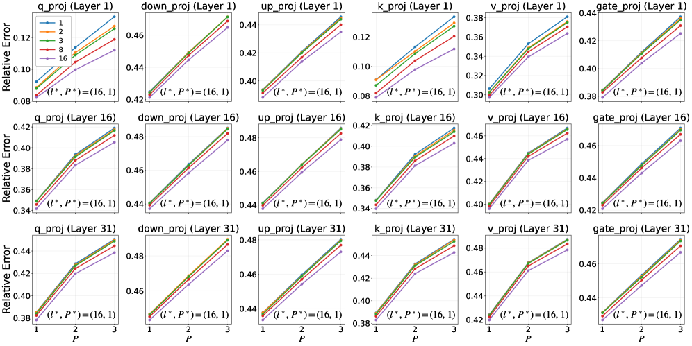
Figure 1: Layer-wise reconstruction error vs. envelope rank and decomposition depth (LLaMA2 7B). We conduct experiments under a 1.5 bit quantization setting and report the relative Frobenius error $\nicefrac{{\|W-\widehat{W}\|_{F}}}{{\|W\|_{F}}}$ of MDBF as a function of the envelope rank $l$ and the decomposition depth $P$, evaluated on three representative Transformer blocks of layers $0$, $15$, and $30$ and central attention/MLP projections. Across layers and modules, larger $l$, which increases magnitude expressivity while sharing sign bases, consistently lowers reconstruction error. In contrast, larger $P$, which adds extra decompositions and sign bases, often worsens reconstruction at matched bits per weight. The best configuration in this sweep is $(l^{\ast},P^{\ast})=(16,1)$.

This paper addresses the DBF bottleneck by explicitly allocating limited expressivity to the critical components at extremely low precision. We propose Multi-Envelope Double Binary Factorization (MDBF), which retains the shared 1-bit sign bases and a deployment-friendly binary fast path while replacing the rank-one magnitude envelope with multiple demodulated envelope modes. Figure 1 shows that increasing the envelope rank $l$ systematically reduces reconstruction error; however, while increasing the residual path $P$, as in LittleBit (lee2025littlebit), is often less effective within a fixed bits-per-weight budget. MDBF adds a small number of real-valued degrees of freedom for magnitude modeling, better aligning with the empirically observed low-rank structure of Transformer weights, which are rarely rank-one. To make MDBF applicable for layer-wise PTQ, we introduce a layer-wise optimization pipeline with closed-form initialization followed by ADMM refinement. Across the LLaMA and Qwen families, MDBF improves perplexity and zero-shot accuracy compared to previous binary formats at matched bits per weight, particularly in the challenging 2–1 bit range, while maintaining the same deployment-friendly binary inference primitive.

Contributions.

• Identifying DBF Bottleneck: We identify the bottleneck as the single envelope constraint. Under a fixed bits-per-weight budget, modeling magnitude variation yields greater accuracy gains than increasing sign diversity.

• Multi-Envelope Generalization of DBF: We propose Multi-Envelope DBF (MDBF), which retains the shared 1-bit sign bases and maintains the same deployment-friendly binary fast path while replacing the rank-one magnitude envelope with a rank-$l$ envelope.

• Initialization and ADMM Refinement for MDBF: We generalize the initialization of LittleBit and the ADMM-based refinement of DBF to a multi-envelope setting. This results in a closed-form initializer and an efficient alternating ADMM refinement procedure.

• Empirical Validation: Across the LLaMA and Qwen model families, MDBF consistently reduces reconstruction error and improves perplexity and zero-shot accuracy compared to prior binary formats at matched BPW.

2 Notation

Vectors are denoted by bold lowercase letters, e.g., ${\bm{x}}$, and matrices by uppercase letters, e.g., $W$. Throughout, $W\in{\mathbb{R}}^{N\times M}$ denotes a real-valued weight matrix. We denote by $\odot$ the Hadamard elementwise product, and for a vector ${\bm{a}}$, let $D_{{\bm{a}}}$ represent the diagonal matrix with $(D_{{\bm{a}}})_{ii}=a_{i}$. We use $\|\cdot\|_{F}$ for the Frobenius norm and $\langle A,B\rangle_{F}\coloneqq\mathrm{Tr}(A^{\top}B)$ for the corresponding Frobenius inner product. For any matrix $A$, its singular values are denoted by $\sigma_{1}(A)\geq\cdots\geq\sigma_{\min(N,M)}(A)\geq 0$. For a target rank $R\leq\min(N,M)$, we denote the rank-$R$ truncated SVD of $W$ as $W_{R}=U_{R}\Sigma_{R}V_{R}^{\top}$, where $U_{R}\in{\mathbb{R}}^{N\times R}$ and $V_{R}\in{\mathbb{R}}^{M\times R}$ have orthonormal columns and $\Sigma_{R}=\mathrm{diag}(\sigma_{1},\dots,\sigma_{R})\in{\mathbb{R}}^{R\times R}$. Finally, the entrywise sign function $\mathrm{sign}(\cdot)$ maps to $\{\pm 1\}$, with $\mathrm{sign}(0)=+1$.

3 Preliminaries

3.1 Low-Rank Approximation

A common approach to model compression exploits the empirically observed approximate low-rank structure of weight matrices. Given a weight matrix $W\in{\mathbb{R}}^{N\times M}$, we approximate it with a rank-$R$ factorization:

$$W\approx UV^{\top},~~U\in{\mathbb{R}}^{N\times R},~V\in{\mathbb{R}}^{M\times R}.$$ (1)

Equivalently, $UV^{\top}$ expresses $W$ as a sum of $R$ rank-one components, $UV^{\top}=\sum_{j=1}^{R}{\bm{u}}_{j}{\bm{v}}_{j}^{\top}$, where ${\bm{u}}_{j}$ and ${\bm{v}}_{j}$ are the $j$-th columns of $U$ and $V$.

However, low rank alone does not guarantee meaningful memory savings. If $U$ and $V$ are stored in standard high-precision formats, such as FP16 or FP32, the parameter count becomes $(N+M)R$, which may be comparable to the original $NM$ parameters unless $R\ll\min(N,M)$. Moreover, maintaining accuracy often requires a moderate $R$, further limiting the compression benefit. Therefore, to achieve significant savings at very low bit widths while maintaining a sufficiently large effective rank, it is crucial to quantize the factors or introduce additional structures that facilitate both compact storage and efficient computation.

3.2 Double Binary Factorization

Double Binary Factorization (DBF) (boza2025dbf) represents a weight matrix $W\in{\mathbb{R}}^{N\times M}$ by utilizing two binary sign bases and diagonal rescalings:

$$\widehat{W}_{\mathrm{DBF}}\coloneqq D_{{\bm{a}}}S_{a}D_{{\bm{m}}}S_{b}^{\top}D_{{\bm{b}}},$$ (2)

where ${\bm{a}}\in{\mathbb{R}}^{N}$ and ${\bm{b}}\in{\mathbb{R}}^{M}$ are the row and column scaling vectors, ${\bm{m}}\in{\mathbb{R}}^{R}$ is an inner scaling vector, and $S_{a}\in\{\pm 1\}^{N\times R}$ and $S_{b}\in\{\pm 1\}^{M\times R}$ are binary sign matrices. Equation (2) can be regarded as a structured rank-$R$ factorization:

$$\widehat{W}_{\mathrm{DBF}}=\widehat{U}\widehat{V}^{\top},\\ \widehat{U}\coloneqq D_{{\bm{a}}}S_{a}D_{{\bm{m}}^{\nicefrac{{1}}{{2}}}},~\widehat{V}\coloneqq D_{{\bm{b}}}S_{b}D_{{\bm{m}}^{\nicefrac{{1}}{{2}}}}.$$ (3)

Single-Envelope Constraint.

For a sign mask $S\in\{\pm 1\}^{p\times q}$ and a matrix $Z\in{\mathbb{R}}^{p\times q}$, we define the demodulated envelope of $Z$ concerning $S$ as $E_{S}(Z)\coloneqq S\odot Z$. In DBF, the demodulated envelopes of factors $\widehat{U}$ and $\widehat{V}$ satisfy the following exact identities:

$$E_{S_{a}}(\widehat{U})=S_{a}\odot\widehat{U}={\bm{a}}({\bm{m}}^{\nicefrac{{1}}{{2}}})^{\top},\\ E_{S_{b}}(\widehat{V})=S_{b}\odot\widehat{V}={\bm{b}}({\bm{m}}^{\nicefrac{{1}}{{2}}})^{\top}.$$ (4)

Therefore, the following holds:

$$\mathrm{rank}(E_{S_{a}}(\widehat{U}))\leq 1,~~\mathrm{rank}(E_{S_{b}}(\widehat{V}))\leq 1,$$ (5)

after demodulation by the shared sign bases, both factor envelopes constitute rank-one outer products. Equivalently, each column of $\widehat{U}$ shares the same row-wise envelope profile ${\bm{a}}$ up to a scalar multiplier $m_{j}^{1/2}$, and similarly ${\bm{b}}$ applies to $\widehat{V}$. We refer to this rank-one demodulated-envelope constraint as the single envelope constraint.

Inference.

Let $X\in{\mathbb{R}}^{T\times N}$ denote the input activations and $Y=X\widehat{W}_{\mathrm{DBF}}\in{\mathbb{R}}^{T\times M}$ the output. DBF admits an efficient evaluation order in which diagonal scalings are interleaved with two binary matrix multiplications:

$$Y=X\widehat{W}_{\mathrm{DBF}}=\Bigl(\Bigl(\Bigl(\bigl(XD_{{\bm{a}}}\bigr)S_{a}\Bigr)D_{{\bm{m}}}\Bigr)S_{b}^{\top}\Bigr)D_{{\bm{b}}}.$$ (6)

Multiplication by a diagonal matrix is equivalent to elementwise rescaling and is typically bandwidth-light compared to matrix multiplication. Therefore, DBF substitutes one high-precision GEMM with two binary GEMMs and inexpensive diagonal operations. The effective bits-per-weight is determined by the storage of bitpacked $\{S_{a},S_{b}\}$ and real-valued vectors $\{{\bm{a}},{\bm{b}},{\bm{m}}\}$, relative to the $NM$ entries of the original matrix.

Residual Compensation.

LittleBit (lee2025littlebit) improves fidelity by augmenting a single DBF approximation with an additional DBF term trained on the residual. LittleBit specifically employs a two-term decomposition as follows:

$$\widehat{W}_{\mathrm{LittleBit}}=D_{{\bm{a}}^{(1)}}S_{a}^{(1)}D_{{\bm{m}}^{(1)}}S_{b}^{(1)\top}D_{{\bm{b}}^{(1)}}\\ +D_{{\bm{a}}^{(2)}}S_{a}^{(2)}D_{{\bm{m}}^{(2)}}S_{b}^{(2)\top}D_{{\bm{b}}^{(2)}}.$$ (7)

A natural optimization strategy is stagewise residual fitting: first, fit the initial term, then compute the residual term:

$$\widehat{R}\coloneqq W-D_{{\bm{a}}^{(1)}}S_{a}^{(1)}D_{{\bm{m}}^{(1)}}S_{b}^{(1)\top}D_{{\bm{b}}^{(1)}}.$$ (8)

Fit the second DBF term to approximate $\widehat{R}$. This residual-compensation scheme captures structures that are difficult to represent with a single DBF component.

4 Method

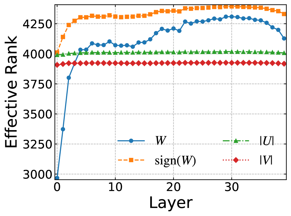
Figure 2: Entropy-based effective rank across Transformer layers for LLaMA2 13B. We report the average effective rank of the full weight matrices $W$, their binarized signs $\mathrm{sign}(W)$, and the demodulated envelopes $|U|$ and $|V|$. The envelopes remain consistently above rank one, indicating multiple magnitude modes and motivating the relaxation of the single-envelope constraint.

4.1 Bottleneck: Single-Envelope Constraint

In practice, DBF exhibits a performance ceiling; increasing the inner dimension $R$ results in diminishing returns, and accuracy saturates below that of a real-valued low-rank approximation with a comparable parameter count. This gap is not merely empirical but structural. As shown in Section 3, demodulation indicates that each DBF factor is constrained by a rank-one amplitude envelope shared across all $R$ columns. Enlarging $R$ primarily increases sign-pattern diversity rather than enhancing the capacity to represent magnitudes, fundamentally limiting achievable accuracy.

The assumption of a rank-one envelope is inconsistent with the empirical structure of LLM weights. To quantify this point, we analyze LLaMA2 13B and compute the entropy-based effective ranks (roy2007effectiveRank) of the demodulated envelopes $|U|$ and $|V|$; see Appendix B.1 for a detailed definition. Figure 2 shows the average effective rank across Transformer blocks and their linear layers. Although the envelopes are low-rank, they are consistently not rank-one; their effective ranks remain moderately above 1, suggesting multiple magnitude modes that DBF cannot represent under the single-envelope constraint.

These observations clarify why merely increasing sign variation, such as in residual-style multi-term designs like LittleBit, is not the most direct solution. The goal is to preserve a deployment-friendly inference path, where shared binary carriers facilitate efficient 1-bit computation while alleviating the bottleneck. This motivation leads to Multi-Envelope DBF, which enhances expressivity by allowing higher-rank amplitude envelopes to be used under the same shared binary sign bases, without altering the inference-time execution model.

4.2 Multi-Envelope Double Binary Factorization

We propose Multi-Envelope DBF (MDBF), which preserves the shared 1-bit sign bases while allowing the demodulated envelopes of the factor matrices to have a rank of at most $l$ as follows:

$$\widehat{W}_{l}\coloneqq\widehat{U}_{l}\widehat{V}_{l}^{\top},\widehat{U}_{l}=S_{a}\odot AQ^{\top},\widehat{V}_{l}=S_{b}\odot BG^{\top},$$ (9)

where $S_{a}\in\{\pm 1\}^{N\times R}$ and $S_{b}\in\{\pm 1\}^{M\times R}$ are binary sign matrices, while $A\in{\mathbb{R}}^{N\times l}$, $Q\in{\mathbb{R}}^{R\times l}$, $B\in{\mathbb{R}}^{M\times l}$, and $G\in{\mathbb{R}}^{R\times l}$ are real-valued factors. By construction, the demodulated envelopes are low-rank:

$$E_{S_{a}}(\widehat{U}_{l})=S_{a}\odot\widehat{U}_{l}=AQ^{\top},\\ E_{S_{b}}(\widehat{V}_{l})=S_{b}\odot\widehat{V}_{l}=BG^{\top},$$ (10)

leads to $\mathrm{rank}(E_{S_{a}}(\widehat{U}_{l}))\leq l$ and $\mathrm{rank}(E_{S_{b}}(\widehat{V}_{l}))\leq l$. Let $A=[{\bm{a}}^{(1)},\dots,{\bm{a}}^{(l)}]$ and $Q=[{\bm{q}}^{(1)},\dots,{\bm{q}}^{(l)}]$, along with $B=[{\bm{b}}^{(1)},\dots,{\bm{b}}^{(l)}]$ and $G=[{\bm{g}}^{(1)},\dots,{\bm{g}}^{(l)}]$, yield the expansions

$$\widehat{U}_{l}=\sum_{t=1}^{l}D_{{\bm{a}}^{(t)}}S_{a}D_{{\bm{q}}^{(t)}},\widehat{V}_{l}=\sum_{s=1}^{l}D_{{\bm{b}}^{(s)}}S_{b}D_{{\bm{g}}^{(s)}}.$$ (11)

Thus, $\widehat{W}_{l}$ admits an equivalent sum-of-DBF form:

$$\widehat{W}_{l}=\sum_{t=1}^{l}\sum_{s=1}^{l}D_{{\bm{a}}^{(t)}}S_{a}D_{{\bm{q}}^{(t)}\odot{\bm{g}}^{(s)}}S_{b}^{\top}D_{{\bm{b}}^{(s)}}.$$ (12)

MDBF generalizes DBF: when $l=1$, Equation (9) reduces to a single DBF term involving ${\bm{m}}={\bm{q}}^{(1)}\odot{\bm{g}}^{(1)}$; if one enforces ${\bm{m}}\geq 0$, ${\bm{q}}^{(1)}={\bm{g}}^{(1)}={\bm{m}}^{\nicefrac{{1}}{{2}}}$ may be set to column-sign absorption in $S_{a},S_{b}$.

4.3 Multi-Envelope Structure

We next formalize the role of envelope rank $l$ and derive the corresponding closed-form optimizer using a fixed sign mask. The key idea is to decompose each factor into (i) a binary sign mask and (ii) a demodulated envelope, while imposing a rank constraint on the envelope.

Demodulation under Fixed Sign Mask.

Fix a sign mask $S\in\{\pm 1\}^{N\times R}$ and consider an arbitrary factor matrix $U\in{\mathbb{R}}^{N\times R}$. We define the demodulated envelope as follows:

$$E_{S}(U)\coloneqq S\odot U.$$ (13)

Since $S_{ij}^{2}=1$ holds for all $(i,j)$, we obtain $S\odot(S\odot Z)=Z$ for any matrix $Z$. Thus, once $S$ is fixed, $U$ is determined by its envelope $E_{S}(U)$.

Consider an approximation $\widehat{U}$ that shares the same mask $S$. It can be expressed as $\widehat{U}=S\odot\widehat{E}$ for some envelope matrix $\widehat{E}\in{\mathbb{R}}^{N\times R}$. Moreover, by Lemma A.3, the mapping $Z\mapsto S\odot Z$ preserves Frobenius norms:

$$\|U-\widehat{U}\|_{F}=\|E_{S}(U)-\widehat{E}\|_{F}.$$ (14)

Therefore, under a fixed mask $S$, approximating $U$ in Frobenius norm is equivalent to approximating its demodulated envelope.

Rank-$l$ Envelope Class.

MDBF constrains the envelope to a low rank. For $l\geq 1$, we define the feasible family as follows:

Definition 4.1.

Let $S\in\{\pm 1\}^{N\times R}$ and $l\geq 1$. Define

$${\mathcal{F}}_{l}(S)\coloneqq\ab\{S\odot E\mid E\in{\mathbb{R}}^{N\times R},\mathrm{rank}(E)\leq l\}.$$ (15)

Equivalently, $\widehat{U}\in{\mathcal{F}}_{l}(S)$ if and only if its envelope $E_{S}(\widehat{U})=S\odot\widehat{U}$ has a rank of at most $l$. This implies the MDBF factor structure; for example, $\widehat{U}_{l}=S_{a}\odot(AQ^{\top})$ satisfies $\mathrm{rank}(E_{S_{a}}(\widehat{U}_{l}))=\mathrm{rank}(AQ^{\top})\leq l$.

Closed-form Minimizer.

By Equation (14), the best approximation of $U$ within ${\mathcal{F}}_{l}(S)$ becomes the classical best rank-$l$ approximation problem for the envelope matrix $E_{S}(U)$. The following theorem demonstrates this equivalence and provides both the optimal error and a minimizer.

Theorem 4.2.

Let $U\in{\mathbb{R}}^{N\times R}$ fix a sign mask $S\in\{\pm 1\}^{N\times R}$. Let $\sigma_{1}(E_{S}(U))\geq\cdots\geq\sigma_{\min(N,R)}(E_{S}(U))\geq 0$ be the singular values of $E_{S}(U)=S\odot U$. Fix an integer $l$ such that $1\leq l\leq\min(N,R)$. Then

$$\min_{\widehat{U}\in{\mathcal{F}}_{l}(S)}\|U-\widehat{U}\|_{F}=\ab(\sum_{i=l+1}^{\min(N,R)}\sigma_{i}\bigl(E_{S}(U)\bigr)^{2})^{\nicefrac{{1}}{{2}}}.$$ (16)

Moreover, one minimizer is

$$\widehat{U}^{\ast}=S\odot\mathrm{TSVD}_{l}(E_{S}(U)),$$ (17)

where $\mathrm{TSVD}_{l}(\cdot)$ denotes the rank-$l$ truncated SVD, which provides the best approximation in the Frobenius norm.

The minimizer Equation (17) directly follows from Equation (14). Writing $\widehat{U}=S\odot\widehat{E}$ with $\mathrm{rank}(\widehat{E})\leq l$ yields $\|U-\widehat{U}\|_{F}=\|E_{S}(U)-\widehat{E}\|_{F}$, thereby identifying the optimal choice as the best rank-$l$ approximation $\widehat{E}=\mathrm{TSVD}_{l}(E_{S}(U))$ according to the Eckart–Young–Mirsky theorem; remodulating with $S$ results in Equation (17).

Theorem 4.2 clarifies the role of $l$: for a fixed binary basis $S$, MDBF approximates the demodulated envelope $E_{S}(U)$ using a rank-$l$ matrix and then reattaches the same mask. Thus, MDBF does not allocate additional degrees of freedom to sign patterns; rather, it enhances capacity by permitting multiple envelope modes in the demodulated domain. DBF represents the special case $l=1$, which constrains the envelope to rank-one and requires all $R$ columns to share a single envelope direction up to scalar weights. For $l>1$, the feasible set strictly expands, ${\mathcal{F}}_{1}(S)\subseteq{\mathcal{F}}_{l}(S)$, and the optimal error in Equation (16) can only decrease.

4.4 Layer-Wise Optimization

We adopt a layer-wise PTQ setting, in which we quantize each weight matrix $W\in{\mathbb{R}}^{N\times M}$ independently under strict memory and computational constraints. Even with the binary sign bases fixed, optimizing MDBF remains non-convex; the objective is bilinear in the factor matrices, and we impose low-rank constraints on their demodulated envelopes. We propose a two-stage pipeline: (i) a closed-form initialization based on Multi-Envelope SVID (MSVID) and (ii) local refinement using alternating updates of ADMM. The resulting factors also provide a robust warmup start for QAT.

4.4.1 Initialization via Multi-Envelope SVID

We begin by defining the operator used in both initialization and refinement. For any matrix $Z\in{\mathbb{R}}^{N\times M}$ and any $l$ with $1\leq l\leq\min(N,M)$, define

$$\mathrm{MSVID}_{l}[Z]\coloneqq\mathrm{sign}(Z)\odot\mathrm{TSVD}_{l}(|Z|).$$ (18)

Equivalently, let $S_{Z}\coloneqq\mathrm{sign}(Z)$, and noting that the demodulated envelope satisfies $E_{S_{Z}}(Z)=S_{Z}\odot Z=|Z|$, the operator $\mathrm{MSVID}_{l}[Z]$ preserves the sign mask $S_{Z}$ while replacing the envelope with its optimal rank-$l$ approximation. The special case $l=1$ corresponds to a rank-one envelope.

Given $W\in{\mathbb{R}}^{N\times M}$ and an inner dimension $R$ with $1\leq R\leq\min(N,M)$, we first compute the rank-$R$ truncated SVD, $W_{R}=U_{R}\Sigma_{R}V_{R}^{\top}$, to form balanced factors

$$U_{0}\coloneqq U_{R}\Sigma_{R}^{\nicefrac{{1}}{{2}}}\in{\mathbb{R}}^{N\times R},~V_{0}\coloneqq V_{R}\Sigma_{R}^{\nicefrac{{1}}{{2}}}\in{\mathbb{R}}^{M\times R},$$ (19)

so that $W_{R}=U_{0}V_{0}^{\top}$. We then initialize MDBF by applying Equation (18) to each continuous factor:

$$\widehat{U}_{l}^{(0)}\coloneqq\mathrm{MSVID}_{l}[U_{0}],~\widehat{V}_{l}^{(0)}\coloneqq\mathrm{MSVID}_{l}[V_{0}].$$ (20)

By construction, $\widehat{U}_{l}^{(0)}$ and $\widehat{V}_{l}^{(0)}$ possess rank-$l$ demodulated envelopes under their induced sign masks, conforming to the MDBF factor structure.

4.4.2 ADMM Refinement

Starting from $\widehat{W}^{(0)}=\widehat{U}_{l}^{(0)}\widehat{V}_{l}^{(0)\top}$, we refine the factors through alternating updates that minimize the reconstruction objective $\|W-UV^{\top}\|_{F}^{2}$ while repeatedly imposing the multi-envelope structure via $\mathrm{MSVID}_{l}[\cdot]$. Specifically, with $V$ fixed, we conduct a limited number of ADMM inner iterations using an auxiliary variable $\widetilde{U}$ and a scaled dual variable $\Lambda$:

$$\widetilde{U}^{(k+1)} =\ab(WV^{(k)}+\rho(U^{(k)}-\Lambda^{(k)}))$$ (21)

$$\times\ab(V^{(k)\top}V^{(k)}+\rho I)^{-1},$$ (22)

$$U^{(k+1)} =\mathrm{MSVID}_{l}\ab[\widetilde{U}^{(k+1)}+\Lambda^{(k)}],$$ (23)

$$\Lambda^{(k+1)} =\Lambda^{(k)}+\widetilde{U}^{(k+1)}-U^{(k+1)},$$ (24)

where $\rho>0$ and $I$ are the $R\times R$ identity matrix. We update $V$ analogously by applying the same steps to the transposed problem while keeping $U$ fixed.

Since $\mathrm{MSVID}_{l}[\cdot]$ updates the sign mask via $\mathrm{sign}(\cdot)$, it is not an exact Frobenius projection onto any fixed-mask constraint set, and standard ADMM convergence guarantees do not apply directly. Therefore, we consider the method as an ADMM-inspired scheme that alternates between closed-form least-squares updates and a mask-adaptive rank-$l$ envelope step. Crucially, Theorem 4.2 provides the theoretical backbone: with strong initialization, subsequent updates function as a refinement mechanism that improves the solution in practice.

5 Experiments

Table 1: Perplexities ($\downarrow$) on WikiText2 for each model. Rows indicate the target bitwidth, and columns correspond to bit-parameters $(l,P)$. DBF uses the same parameter format as $(l,P)=(1,1)$, and LittleBit uses the same format as $(l,P)=(1,2)$.

Model	Bits	$(l{=}1,P{=}1)$	$(l{=}1,P{=}2)$	$(l{=}2,P{=}1)$	$(l{=}8,P{=}1)$	$(l{=}16,P{=}1)$
Tiny LLaMA (1.1B)	1.00	78.14	114.84	blue!570.17	blue!570.04	blue!560.40
	1.25	21.96	37.71	blue!522.50	blue!521.67	blue!519.98
	1.50	15.85	19.85	blue!516.41	blue!514.94	blue!514.27
Qwen3 (0.6B)	1.00	343.80	773.01	blue!5415.91	blue!5262.56	blue!5277.12
	1.25	120.89	221.01	blue!5121.23	blue!5128.35	blue!5111.70
	1.50	100.84	121.72	blue!578.77	blue!585.15	blue!570.97
LLaMA3.2 (1B)	1.00	118.69	131.20	blue!5118.17	blue!5119.82	blue!5104.28
	1.25	47.99	84.12	blue!542.35	blue!539.88	blue!541.46
	1.50	47.78	44.90	blue!539.50	blue!541.06	blue!538.54
LLaMA2 (7B)	1.00	27.96	37.92	blue!528.01	blue!529.72	blue!528.31
	1.25	13.40	21.67	blue!512.82	blue!515.83	blue!518.26
	1.50	9.81	12.14	blue!59.83	blue!59.94	blue!510.50
LLaMA3 (8B)	1.00	1222.32	9118.75	blue!51024.80	blue!52094.86	blue!51639.64
	1.25	58.61	165.43	blue!550.13	blue!592.02	blue!5164.24
	1.50	35.62	41.40	blue!536.11	blue!530.14	blue!531.70
Qwen3 (8B)	1.00	189.02	309.30	blue!5108.90	blue!5134.00	blue!5115.41
	1.25	41.10	101.54	blue!553.24	blue!563.73	blue!569.18
	1.50	31.72	39.02	blue!540.22	blue!530.09	blue!532.28

5.1 Setting

Baselines and Quantization Methods.

We use representative low-rank binary-factor formats as baselines: DBF, corresponding to $(l,P)=(1,1)$, and LittleBit, corresponding to $(l,P)=(1,2)$. For each method, we optimize the binary-factor parameters using ADMM for 1,000 outer iterations, with 3 inner ADMM updates per outer step. For formats utilizing $P$ decomposed terms, we apply this ADMM procedure independently for each term, resulting in a total of $1{,}000\times P$ outer iterations. Following ADMM, we perform an additional gradient-based refinement using Adam for 1,500 steps, with a learning rate of $0.01$. During this refinement stage, we update only the real-valued parameters by minimizing the squared reconstruction loss $\|W-\widehat{W}\|_{F}^{2}$. For each target bit budget of $\{1.00,1.25,1.50\}$ bits per weight, we choose the largest inner rank that meets the budget, following boza2025dbf.

To enhance accuracy in the low-bit regime, we incorporate an error-compensation technique. Specifically, we adopt quantization error propagation (QEP) (arai2025quantization) with $\alpha=0.5$ and use 512 samples from WikiText2 to estimate the required statistics. Finally, in line with standard practice, we retain the first four and last four layers in full precision to ensure a fair and stable comparison across methods.

Models and Datasets.

We evaluate the proposed low-rank binary-factor format and baseline variants on widely used open-weight LLM families, including LLaMA2 (touvron2023llama), LLaMA3 (grattafiori2024llama), and Qwen. Specifically, we analyze the standard benchmarks of Tiny LLaMA 1.1B, LLaMA2 7B, LLaMA3 8B, and LLaMA3.2 1B in prior quantization work (boza2025dbf). To assess robustness across architectural variations, we also evaluate Qwen3 0.6B and Qwen3 8B, which differ from LLaMA models by incorporating RMSNorm variants in their attention components.

Evaluation.

We follow established evaluation practices for LLM quantization (boza2025dbf; lee2025littlebit). We report perplexity (PPL) on WikiText2 and evaluate downstream zero-shot performance on ARC-Easy, and PIQA. In the main text, we present the average accuracy across tasks and include per-task results in Appendix C. All experiments were conducted on a single NVIDIA B200 GPU.

5.2 Result

Table 2: Average zero-shot accuracy ($\uparrow$) on ARC-Easy and PIQA. Rows indicate the target bitwidth, and columns correspond to bit-parameters $(l,P)$. Notably, DBF uses the same parameter format as $(l,P)=(1,1)$, and LittleBit uses the same format as $(l,P)=(1,2)$.

Model	Bits	$(l{=}1,P{=}1)$	$(l{=}1,P{=}2)$	$(l{=}2,P{=}1)$	$(l{=}8,P{=}1)$	$(l{=}16,P{=}1)$
Tiny LLaMA (1.1B)	1.00	0.4398	0.4355	blue!50.4423	blue!50.4557	blue!50.4449
	1.25	0.4945	0.4608	blue!50.5049	blue!50.5045	blue!50.5179
	1.50	0.5252	0.5053	blue!50.5273	blue!50.5311	blue!50.5259
Qwen3 (0.6B)	1.00	0.4237	0.4110	blue!50.4244	blue!50.4120	blue!50.4228
	1.25	0.4390	0.4213	blue!50.4449	blue!50.4449	blue!50.4457
	1.50	0.4519	0.4317	blue!50.4604	blue!50.4544	blue!50.4609
LLaMA3.2 (1B)	1.00	0.4639	0.4716	blue!50.4691	blue!50.4680	blue!50.4691
	1.25	0.4977	0.4842	blue!50.5039	blue!50.5196	blue!50.5099
	1.50	0.5082	0.5202	blue!50.5222	blue!50.5386	blue!50.5240
LLaMA2 (7B)	1.00	0.5263	0.4919	blue!50.5217	blue!50.5229	blue!50.5229
	1.25	0.5981	0.5522	blue!50.6096	blue!50.5767	blue!50.5785
	1.50	0.6398	0.6110	blue!50.6480	blue!50.6243	blue!50.6341
LLaMA3 (8B)	1.00	0.4078	0.3997	blue!50.4104	blue!50.4185	blue!50.4095
	1.25	0.4796	0.4370	blue!50.5004	blue!50.4716	blue!50.4443
	1.50	0.5208	0.5056	blue!50.5059	blue!50.5069	blue!50.5000
Qwen3 (8B)	1.00	0.4635	0.4508	blue!50.4588	blue!50.4486	blue!50.4589
	1.25	0.4971	0.4646	blue!50.4993	blue!50.4819	blue!50.4854
	1.50	0.5186	0.4880	blue!50.5159	blue!50.5263	blue!50.5119

Reconstruction Error.

A central motivation for MDBF is that, under an extremely tight bit budget, additional sign diversity may inefficiently utilize capacity compared to enhancing magnitude expressivity. We investigate this by analyzing how layer-wise reconstruction error depends on (i) the envelope rank $l$, which increases magnitude capacity while keeping the shared binary sign bases, and (ii) the residual path $P$, which introduces extra factor terms and additional sign bases, as seen in residual binary decompositions (boza2025dbf; lee2025littlebit). We evaluate LLaMA2-7B on three representative Transformer blocks (layers $0$, $15$, and $30$) and compute the reconstruction error for the attention and MLP projection matrices. For each weight matrix $W$ and its quantized approximation $\widehat{W}$, we report the relative Frobenius error $\nicefrac{{\|W-\widehat{W}\|_{F}}}{{\|W\|_{F}}}$ while sweeping $l\in\{1,2,3,8,16\}$ and $P\in\{1,2,3\}$ at matched bits per weight. Although larger envelope ranks, e.g., $l\geq 16$, may further improve performance, we defer these settings to future work due to their higher computational cost; notably, $l=16$ is sufficient to demonstrate their effectiveness.

Figure 1 shows a consistent trend across layers and modules. For any fixed $P$, increasing $l$ reduces reconstruction error, whereas increasing $P$ is generally ineffective within the same bit budget. This behavior supports the design choice of MDBF: to reuse a shared binary carrier and allocate the limited capacity to a richer magnitude structure, rather than duplicating sign bases. In contrast, a larger $P$ necessitates the storage of additional sign matrices, diverting bits from magnitude modeling and potentially increasing approximation error. The effect is strongest in the earliest block, where the gap across $(l,P)$ is most significant among several projections. Since quantization noise introduced early can propagate through the network, minimizing errors in the early layers is particularly important.

Perplexity and Zero-shot Accuracy.

Table 1 demonstrates that MDBF is the strongest across models when comparing matched bits-per-weight, resulting in consistent reductions in perplexity. Notably, the improvements are most significant in the extremely low bit regime. Table 2 also presents downstream zero-shot performance and displays trends closely aligned with those in Table 1.

Across a fixed bit budget, we find that increasing the envelope rank $l$ contributes more to performance than increasing $P$. Specifically, larger $l$ yields improvements in both perplexity and zero-shot accuracy, while larger $P$ provides more modest enhancements. In this regime, our method significantly outperforms the baselines, often by a substantial margin. By contrast, for larger models around the 7B scale, the gains begin to saturate. We observe that the quantization error continues to decline, suggesting that the method may be overfitting the calibration data instead of translating these improvements into downstream gains. Exploring whether these trends persist with significantly larger calibration sets is an important direction for future work.

6 Related Work

Post-Training Quantization at $\sim$4 Bits.

Most practical low-bit deployments of LLMs rely on PTQ in the roughly 4-bit range. Layer-wise calibration methods, such as GPTQ (li2025gptaq; frantar2022gptq) and AWQ (lin2024awq), achieve strong accuracy without full retraining by minimizing layer-wise reconstruction errors or by identifying and preserving salient weight channels during calibration. However, when the bit budget increases to $\leq 2$ bits per weight, these techniques often result in significant accuracy degradation, underscoring the need for more structured parameterizations.

Structured Representations for 2–3 Bits.

To achieve the 2–3 bit regime, recent studies often go beyond purely elementwise quantization to adopt structured weight representations. A representative line combines incoherence processing with lattice- and trellis-coded quantizers, as seen in QuIP# (tseng2024quip), QTIP (tseng2024qtip), and AQLM (egiazarian2024aqlm). By encoding weights using structured codebooks instead of independent rounding, these methods enhance effective expressivity within tight bit budgets. In this regime, heuristic STE-based adjustments tend to be unstable (long2021learning; ichikawa2025high; yin2019understanding); therefore, refinement is typically framed as a discrete optimization problem (malinovskii2024pv).

Methods Targeting 1 Bit and Below.

At or below 1 bit precision, maintaining model quality generally requires more flexibility than naive rounding permits. Representative approaches include SVID-based parameterizations (xu2024onebit), token-adaptive mixtures of scaling factors (jo2024binarymos), and structured sparsity (dong2025stbllm). In parallel, binary-factor formats maintain efficient inference primitives (boza2025dbf; lee2025littlebit) by decomposing each weight matrix into two bit-packed sign matrices with low-cost diagonal scaling, resulting in inference primarily governed by 1-bit kernels. A common theme is the explicit addition of degrees of freedom, such as adaptive scales, learnable sparsity patterns, or residual corrections, to mitigate the information bottleneck caused by extreme quantization.

7 Conclusion

We study extreme low-bit quantization using binary-factor representations and identify a key limitation of DBF: after sign demodulation, all weight magnitudes are constrained to a single shared envelope. This collapse significantly constrains expressivity and leads to diminishing returns as the inner rank increases, explaining the observed performance saturation. To address this bottleneck, we introduce MDBF, which enables deployment-friendly binary computation by preserving shared 1-bit sign bases while replacing the single-envelope with a rank-$l$ demodulated envelope that can represent multiple magnitude modes. We present a practical layer-wise PTQ pipeline featuring closed-form initialization followed by an alternating refinement procedure. Experiments across the LLaMA and Qwen model families demonstrate that MDBF improves perplexity and zero-shot accuracy compared to prior binary formats with the same bits per weight, highlighting that limited capacity is more effectively allocated to modeling magnitudes rather than replicating sign patterns.

8 Limitations

We focus on layer-wise PTQ. Accordingly, we do not consider submodule-level (ichikawa2025lpcd) or block-wise (tseng2024quip; lee2025littlebit) quantization, end-to-end QAT, or distillation-based methods such as LittleBit (lee2025littlebit). While these alternatives may yield additional accuracy gains, they typically require significantly greater computational resources and introduce nontrivial engineering overhead. Our approach minimizes a non-convex objective through heuristic alternating updates. As a result, we do not provide guarantees of global optimality; the best-performing hyperparameter settings, e.g., envelope rank $l$ and decomposition depth $P$, may depend on the optimizer and initialization. Developing more principled optimization strategies or employing robust discrete general optimization methods (ichikawa2025continuous; ichikawa2025optimization; sun2023revisiting; ichikawa2024controlling) and model-selection criteria for extremely low-bit binary-factor formats remains an important open problem.

Appendix A Derivation

A.1 Proofs of Main Results

This section presents detailed proofs of the results stated in the main text, along with the necessary auxiliary lemmas for completeness.

A.1.1 Demodulated envelopes and Envelope Class

Demodulated Envelope.

Let $S\in\{\pm 1\}^{p\times q}$ represent a sign mask and $Z\in{\mathbb{R}}^{p\times q}$ an arbitrary matrix. We define the demodulated envelope of $Z$ concerning $S$ as follows:

$$E_{S}(Z)\coloneqq S\odot Z,$$ (25)

Since $S_{ij}^{2}=1$ holds for all $(i,j)$, we have $S\odot S=\mathbf{1}$ entrywise; therefore, $Z=S\odot E_{S}(Z)$.

Envelope Class.

We recall the rank-$l$ envelope class associated with a fixed sign mask.

Definition A.1.

Let $S\in\{\pm 1\}^{p\times q}$ and $l\geq 1$. Define

$${\mathcal{F}}_{l}(S)\coloneqq\left\{S\odot E\mid E\in{\mathbb{R}}^{p\times q},\mathrm{rank}(E)\leq l\right\}\subset{\mathbb{R}}^{p\times q}.$$ (26)

Equivalently, $\widehat{Z}\in{\mathcal{F}}_{l}(S)$ if and only if its demodulated envelope $E_{S}(\widehat{Z})$ has a rank of at most $l$.

The next lemma demonstrates that ${\mathcal{F}}_{l}(S)$ can be equivalently characterized as a sum of diagonal scalings of the fixed mask $S$, thereby relating envelopes to DBF-like parameterizations.

Lemma A.2.

Let $S\in\{\pm 1\}^{p\times q}$ and $l\geq 1$. Then

$${\mathcal{F}}_{l}(S)=\left\{\sum_{t=1}^{l}D_{{\bm{x}}^{(t)}}SD_{{\bm{y}}^{(t)}}\mid{\bm{x}}^{(t)}\in{\mathbb{R}}^{p},{\bm{y}}^{(t)}\in{\mathbb{R}}^{q}\right\}.$$ (27)

Proof.

We prove both inclusions. Let $\widehat{Z}\in{\mathcal{F}}_{l}(S)$. By Definition A.1, there exists $E\in{\mathbb{R}}^{p\times q}$ such that $\mathrm{rank}(E)\leq l$ with $\widehat{Z}=S\odot E$. Since $\mathrm{rank}(E)\leq l$, there exist vectors $\{{\bm{x}}^{(t)}\}_{t=1}^{l}\subset{\mathbb{R}}^{p}$ and $\{{\bm{y}}^{(t)}\}_{t=1}^{l}\subset{\mathbb{R}}^{q}$ such that $E=\sum_{t=1}^{l}{\bm{x}}^{(t)}({\bm{y}}^{(t)})^{\top}.$ For any $(i,j)$, we compute

$$\widehat{Z}_{ij} =(S\odot E)_{ij}=S_{ij}E_{ij}=S_{ij}\sum_{t=1}^{l}x_{i}^{(t)}y_{j}^{(t)}=\sum_{t=1}^{l}x_{i}^{(t)}S_{ij}y_{j}^{(t)}=\sum_{t=1}^{l}\bigl(D_{{\bm{x}}^{(t)}}SD_{{\bm{y}}^{(t)}}\bigr)_{ij}.$$ (28)

Therefore, $\widehat{Z}=\sum_{t=1}^{l}D_{{\bm{x}}^{(t)}}SD_{{\bm{y}}^{(t)}}$, which shows that $\widehat{Z}$ belongs to the right-hand side of Equation (27). Suppose that $\widehat{Z}=\sum_{t=1}^{l}D_{{\bm{x}}^{(t)}}SD_{{\bm{y}}^{(t)}}$. Define $E\coloneqq\sum_{t=1}^{l}{\bm{x}}^{(t)}\bigl({\bm{y}}^{(t)}\bigr)^{\top}$. Then $\mathrm{rank}(E)\leq l$. Moreover, for any $(i,j)$,

$$(S\odot E)_{ij} =S_{ij}E_{ij}=S_{ij}\sum_{t=1}^{l}x_{i}^{(t)}y_{j}^{(t)}=\sum_{t=1}^{l}x_{i}^{(t)}S_{ij}y_{j}^{(t)}=\sum_{t=1}^{l}\bigl(D_{{\bm{x}}^{(t)}}SD_{{\bm{y}}^{(t)}}\bigr)_{ij}=\widehat{Z}_{ij}.$$ (29)

Hence, $\widehat{Z}=S\odot E\in{\mathcal{F}}_{l}(S)$ completes the proof. ∎

A.1.2 Isometry Induced by Sign Mask

Lemma A.3.

Let $S\in\{\pm 1\}^{p\times q}$ and $A,B\in{\mathbb{R}}^{p\times q}$.

$$\|S\odot A\|_{F}=\|A\|_{F},~~\|S\odot(A-B)\|_{F}=\|A-B\|_{F}.$$ (30)

The linear map $T_{S}:{\mathbb{R}}^{p\times q}\to{\mathbb{R}}^{p\times q}$ defined by $T_{S}(Z)\coloneqq S\odot Z$ is an isometry with respect to $\|\cdot\|_{F}$.

Proof.

Using the definition of the Frobenius norm and the fact that $S_{ij}^{2}=1$ for all $(i,j)$, we have

$$\|S\odot A\|_{F}^{2} =\sum_{i=1}^{p}\sum_{j=1}^{q}(S_{ij}A_{ij})^{2}=\sum_{i=1}^{p}\sum_{j=1}^{q}S_{ij}^{2}\,A_{ij}^{2}=\sum_{i=1}^{p}\sum_{j=1}^{q}A_{ij}^{2}=\|A\|_{F}^{2}.$$ (31)

Taking the square roots yields $\|S\odot A\|_{F}=\|A\|_{F}$. Applying the same argument to $A$-$B$ yields

$$\|S\odot(A-B)\|_{F}=\|A-B\|_{F},$$ (32)

which establishes the distance-preservation property and, consequently, the isometry claim. ∎

A.1.3 Optimal Demodulated-Envelope Approximation

We restate and prove Theorem 4.2 from the perspective of the demodulated-envelope.

Theorem A.4.

Let $U\in{\mathbb{R}}^{N\times R}$ fix a sign mask $S\in\{\pm 1\}^{N\times R}$. Let $\sigma_{1}(E_{S}(U))\geq\cdots\geq\sigma_{\min(N,R)}(E_{S}(U))\geq 0$ denote the singular values of the demodulated envelope $E_{S}(U)\coloneqq S\odot U$. Fix an integer $l$ with $1\leq l\leq\min(N,R)$. Then

$$\min_{\widehat{U}\in{\mathcal{F}}_{l}(S)}\|U-\widehat{U}\|_{F}^{2}=\sum_{i=l+1}^{\min(N,R)}\sigma_{i}\bigl(E_{S}(U)\bigr)^{2}.$$ (33)

Moreover, a minimizer is provided by

$$\widehat{U}^{\star}=S\odot\mathrm{TSVD}_{l}\bigl(E_{S}(U)\bigr),$$ (34)

where $\mathrm{TSVD}_{l}(\cdot)$ denotes the best rank-$l$ approximation in the Frobenius norm.

Proof.

By Definition 4.1, $\widehat{U}\in{\mathcal{F}}_{l}(S)$ if and only if there exists a matrix $E\in{\mathbb{R}}^{N\times R}$ such that $\mathrm{rank}(E)\leq l$ as follows:

$$\widehat{U}=S\odot E.$$ (35)

Hence, the constrained minimization over $\widehat{U}\in{\mathcal{F}}_{l}(S)$ is equivalent to minimizing over $E$ with $\mathrm{rank}(E)\leq l$ under the parameterization in Equation (35). Define $E_{U}\coloneqq E_{S}(U)=S\odot U$. Since $S_{ij}^{2}=1$ for all $(i,j)$, we have the involution property $S\odot(S\odot Z)=Z$ for any $Z$, particularly $U=S\odot E_{U}$. For any feasible $\widehat{U}=S\odot E$, we obtain $U-\widehat{U}=S\odot(E_{U}-E)$. Applying Lemma A.3 yields

$$\|U-\widehat{U}\|_{F}=\|E_{U}-E\|_{F},~~\|U-\widehat{U}\|_{F}^{2}=\|E_{U}-E\|_{F}^{2}.$$ (36)

Substituting Equations (35) and (36) gives

$$\min_{\widehat{U}\in{\mathcal{F}}_{l}(S)}\|U-\widehat{U}\|_{F}^{2}=\min_{\begin{subarray}{c}E\in{\mathbb{R}}^{N\times R}\\ \mathrm{rank}(E)\leq l\end{subarray}}\|E_{U}-E\|_{F}^{2},$$ (37)

which is exactly the classical best rank-$l$ approximation problem for $E_{U}$ in Frobenius norm. By the Eckart–Young–Mirsky theorem applied to $E_{U}$, we have

$$\min_{\mathrm{rank}(E)\leq l}\|E_{U}-E\|_{F}^{2}=\sum_{i=l+1}^{\min(N,R)}\sigma_{i}(E_{U})^{2}=\sum_{i=l+1}^{\min(N,R)}\sigma_{i}\bigl(E_{S}(U)\bigr)^{2},$$ (38)

which proves Equation (33). Moreover, the same theorem implies that an optimizer is $E^{\star}=\mathrm{TSVD}_{l}(E_{U})$; substituting into Equation (35) yields $\widehat{U}^{\star}=S\odot\mathrm{TSVD}_{l}(E_{U})=S\odot\mathrm{TSVD}_{l}(E_{S}(U))$, which corresponds to Equation (34). ∎

Remark A.5.

If we choose the mask $S=\mathrm{sign}(U)$, the demodulated envelope satisfies $E_{S}(U)=S\odot U=|U|$ entrywise. In this case, Equation (33) specializes to the standard singular-value tail characterization of the best rank-$l$ approximation error for $|U|$ in the Frobenius norm.

Corollary A.6.

Under the assumptions of Theorem A.4, setting $l=1$ yields

$$\min_{\widehat{U}\in{\mathcal{F}}_{1}(S)}\|U-\widehat{U}\|_{F}^{2}=\sum_{i=2}^{\min(N,M)}\sigma_{i}\bigl(E_{S}(U)\bigr)^{2},.$$ (39)

In particular, the single envelope constraint is lossless (in Frobenius norm) if and only if $\mathrm{rank}\bigl(E_{S}(U)\bigr)\leq 1$.

Proof.

This is the specialization of Theorem A.4 to $l=1$. ∎

A.1.4 Exact Projection

Proposition A.7.

Fix $S\in\{\pm 1\}^{N\times R}$ and $l\geq 1$. For any $Z\in{\mathbb{R}}^{N\times R}$, the Frobenius projection onto ${\mathcal{F}}_{l}(S)$,

$$\Pi_{{\mathcal{F}}_{l}(S)}(Z)\in\arg\min_{Y\in{\mathcal{F}}_{l}(S)}\|Z-Y\|_{F},$$ (40)

selected as

$$\Pi_{{\mathcal{F}}_{l}(S)}(Z)=S\odot\mathrm{TSVD}_{l}\bigl(E_{S}(Z)\bigr)=S\odot\mathrm{TSVD}_{l}\bigl(S\odot Z\bigr).$$ (41)

Proof.

By Definition A.1, any $Y\in{\mathcal{F}}_{l}(S)$ can be expressed as $Y=S\odot E$ for some $E\in{\mathbb{R}}^{N\times R}$ with $\mathrm{rank}(E)\leq l$. Hence,

$$\min_{Y\in{\mathcal{F}}_{l}(S)}\|Z-Y\|_{F}^{2} =\min_{\begin{subarray}{c}E\in{\mathbb{R}}^{N\times R}\\ \mathrm{rank}(E)\leq l\end{subarray}}\|Z-S\odot E\|_{F}^{2}.$$ (42)

Using the sign-mask isometry (Lemma A.3) and the identity $S\odot(S\odot E)=E$, we obtain

$$\|Z-S\odot E\|_{F} =\|S\odot Z-S\odot(S\odot E)\|_{F}=\|S\odot Z-E\|_{F}=\|E_{S}(Z)-E\|_{F}.$$ (43)

Therefore,

$$\min_{Y\in{\mathcal{F}}_{l}(S)}\|Z-Y\|_{F}^{2}=\min_{\mathrm{rank}(E)\leq l}\|E_{S}(Z)-E\|_{F}^{2}.$$ (44)

The right-hand side represents the classical best rank-$l$ approximation problem for $E_{S}(Z)$ in the Frobenius norm, with minimizers provided by the truncated SVD: $E^{\star}=\mathrm{TSVD}_{l}(E_{S}(Z))$ (Eckart–Young–Mirsky theorem). Substituting back yields $Y^{\star}=S\odot E^{\star}=S\odot\mathrm{TSVD}_{l}(E_{S}(Z))$, which is Equation (41). ∎

Appendix B Additional Implementation Details

B.1 Entropy-based effective rank

We quantify the number of envelope modes present using the entropy-based effective rank (entropy rank) (roy2007effectiveRank). For a matrix $E\in{\mathbb{R}}^{N\times M}$ (in our case, a demodulated envelope such as $E_{\mathrm{sign}(U)}(U)=|U|$ or $E_{\mathrm{sign}(V)}(V)=|V|$), let singular values and $\sigma_{1}(E)\geq\cdots\geq\sigma_{\min(N,M)}(E)\geq 0$ represent its normalized spectrum. Define the normalized spectrum

$$\pi_{i}(E)\coloneqq\frac{\sigma_{i}(E)}{\sum_{j=1}^{\min(N,M)}\sigma_{j}(E)},~~~i=1,\dots,\min(N,M),$$ (45)

with the convention $\pi_{i}(E)=1/\min(N,M)$, if $E=0$ and the spectral entropy are considered:

$$H(E)\coloneqq-\sum_{i=1}^{\min(N,M)}\pi_{i}(E)\log\pi_{i}(E).$$ (46)

The effective rank of entropy is $\mathrm{erank}(E)\coloneqq\exp\bigl(H(E)\bigr.)$. This quantity is scale-invariant and satisfies $1\leq\mathrm{erank}(E)\leq\min(N,M)$. Moreover, $\mathrm{erank}(E)=1$ when $E$ is a nonzero rank-one matrix with all spectral mass on a single singular value, and $\mathrm{erank}(E)\approx k$ when roughly $k$ singular values contribute comparably.

Appendix C Additional Experiments

In the main text, we present results aggregated across models (and, where applicable, across tasks) to emphasize overall trends. For completeness and transparency, this appendix includes the individual results for each model and target bitwidth. All experiments follow the same evaluation protocol as the main paper; the reported metric remains the same normalized accuracy (higher is better).

Tables 3 and 4 summarize normalized accuracy on ARC-Easy and PIQA, respectively. Rows indicate the target bit width, while columns correspond to the bit-parameter choices $(l,P)$. Overall, the per-model numbers align with the aggregate results in the main text: changing $(l,P)$ typically results in modest variations, with $(l{=}2,P{=}1)$ providing a strong and stable default across models, while increasing $l$ often leads to diminishing returns.

Table 3: Zero-shot accuracy ($\uparrow$) on ARC-Easy. Rows indicate the target bitwidth, and columns correspond to bit-parameters $(l,P)$.

Model	Bits	$(l{=}1,P{=}1)$	$(l{=}1,P{=}2)$	$(l{=}2,P{=}1)$	$(l{=}8,P{=}1)$	$(l{=}16,P{=}1)$
Tiny LLaMA (1.1B)	1.00	0.3279	0.3258	blue!50.3215	blue!50.3304	blue!50.3283
	1.25	0.3737	0.3384	blue!50.3960	blue!50.3822	blue!50.3927
	1.50	0.4057	0.3838	blue!50.4045	blue!50.4066	blue!50.4082
Qwen3 (0.6B)	1.00	0.3051	0.2883	blue!50.3157	blue!50.2837	blue!50.3064
	1.25	0.3258	0.3089	blue!50.3283	blue!50.3338	blue!50.3245
	1.50	0.3418	0.3140	blue!50.3565	blue!50.3401	blue!50.3485
LLaMA3.2 (1B)	1.00	0.3413	0.3653	blue!50.3359	blue!50.3523	blue!50.3472
	1.25	0.3843	0.3540	blue!50.3897	blue!50.3956	blue!50.3990
	1.50	0.3906	0.4217	blue!50.4112	blue!50.4369	blue!50.4082
LLaMA2 (7B)	1.00	0.4221	0.3842	blue!50.4209	blue!50.4228	blue!50.4265
	1.25	0.5118	0.4482	blue!50.5189	blue!50.4853	blue!50.4899
	1.50	0.5614	0.5240	blue!50.5800	blue!50.5370	blue!50.5631
LLaMA3 (8B)	1.00	0.2879	0.2761	blue!50.3001	blue!50.3077	blue!50.2946
	1.25	0.3628	0.3266	blue!50.3817	blue!50.3544	blue!50.3232
	1.50	0.4099	0.4024	blue!50.3965	blue!50.3864	blue!50.3851
Qwen3 (8B)	1.00	0.3514	0.3439	blue!50.3443	blue!50.3481	blue!50.3514
	1.25	0.4045	0.3645	blue!50.4007	blue!50.3788	blue!50.3805
	1.50	0.4196	0.3885	blue!50.4415	blue!50.4373	blue!50.4188

Table 4: Zero-shot accuracy ($\uparrow$) on PIQA. Rows indicate the target bitwidth, and columns correspond to bit-parameters $(l,P)$.

Model	Bits	$(l{=}1,P{=}1)$	$(l{=}1,P{=}2)$	$(l{=}2,P{=}1)$	$(l{=}8,P{=}1)$	$(l{=}16,P{=}1)$
Tiny LLaMA (1.1B)	1.00	0.5517	0.5452	blue!50.5631	blue!50.5811	blue!50.5615
	1.25	0.6153	0.5832	blue!50.6137	blue!50.6268	blue!50.6431
	1.50	0.6447	0.6268	blue!50.6502	blue!50.6556	blue!50.6436
Qwen3 (0.6B)	1.00	0.5424	0.5337	blue!50.5332	blue!50.5403	blue!50.5392
	1.25	0.5522	0.5337	blue!50.5615	blue!50.5560	blue!50.5669
	1.50	0.5620	0.5495	blue!50.5642	blue!50.5686	blue!50.5734
LLaMA3.2 (1B)	1.00	0.5865	0.5778	blue!50.6023	blue!50.5838	blue!50.5909
	1.25	0.6110	0.6143	blue!50.6181	blue!50.6436	blue!50.6208
	1.50	0.6257	0.6186	blue!50.6333	blue!50.6404	blue!50.6398
LLaMA2 (7B)	1.00	0.6306	0.5997	blue!50.6225	blue!50.6230	blue!50.6192
	1.25	0.6844	0.6561	blue!50.7002	blue!50.6681	blue!50.6670
	1.50	0.7182	0.6980	blue!50.7160	blue!50.7116	blue!50.7051
LLaMA3 (8B)	1.00	0.5277	0.5234	blue!50.5207	blue!50.5294	blue!50.5245
	1.25	0.5963	0.5473	blue!50.6192	blue!50.5887	blue!50.5653
	1.50	0.6317	0.6088	blue!50.6153	blue!50.6273	blue!50.6148
Qwen3 (8B)	1.00	0.5756	0.5577	blue!50.5734	blue!50.5490	blue!50.5664
	1.25	0.5898	0.5647	blue!50.5979	blue!50.5849	blue!50.5903
	1.50	0.6175	0.5876	blue!50.5903	blue!50.6153	blue!50.6050