Computing Flux-Surface Shapes in Tokamaks and Stellarators

Abstract

There is currently no agreed-upon methodology for characterizing a stellarator magnetic field geometry, and yet modern stellarator designs routinely attain high levels of magnetic-field quasi-symmetry through careful flux-surface shaping. Here, we introduce a general method for computing the shape of an ideal-MHD equilibrium that can be used in both axisymmetric and non-axisymmetric configurations. This framework uses a Fourier mode analysis to define the shaping modes (e.g. elongation, triangularity, squareness, etc.) of cross-sections that can be non-planar. Relative to an axisymmetric equilibrium, the additional degree of freedom in a non-axisymmetric equilibrium manifests as a rotation of each shaping mode about the magnetic axis.

Using this method, a shaping analysis is performed on non-axisymmetric configurations with precise quasi-symmetry and select cases from the QUASR database spanning a range of quasi-symmetry quality. Empirically, we find that quasi-symmetry results from a spatial resonance between shape complexity and shape rotation about the magnetic axis. The quantitative features of this resonance correlate closely with a configuration’s rotational transform and number of field periods. Based on these observations, it is conjectured that this shaping paradigm can facilitate systematic investigations into the relationship between general flux-surface geometries and other figures of merit.

I Introduction

In magnetic confinement fusion (MCF), the design and shape of the magnetic field plays a significant role in plasma confinement, influencing a wide range of phenomena that includes magnetohydrodynamic (MHD) stability Scarabosio et al. (2007); Brunetti et al. (2020); Rodríguez (2023), fast-ion confinement Bindel et al. (2023), neoclassical transport Beidler et al. (2021); Canik et al. (2007a, b), and turbulence Angelino et al. (2009); Mynick et al. (2010); Xanthopoulos et al. (2014); Proll et al. (2015); Hegna et al. (2018); Terry et al. (2018); Fontana et al. (2017); Huang et al. (2018); Laribi et al. (2021); Nakata and Matsuoka (2022); Mackenbach et al. (2022); Roberg-Clark et al. (2022); Merlo et al. (2023); Gerard et al. (2023, 2024); Goodman et al. (2024). In tokamaks, where the magnetic field is axisymmetric, the relationship between magnetic geometry and plasma dynamics can be investigated using, for instance, the so-called Miller parameters, which provide a geometric description of the axisymmetric poloidal cross-section with parameters like elongation, triangularity, and squareness Miller et al. (1998). Importantly, this approach has allowed for the systematic investigation into the effect of shaping on the resulting plasma dynamics in both experiment and simulation Weisen et al. (1997); Waltz and Miller (1999); Reimerdes et al. (2000); Scarabosio et al. (2007); Ball and Parra (2017); Fontana et al. (2017); Marinoni et al. (2021); Beeke et al. (2021).

In the (non-axisymmetric) stellarator, however, there is currently no such shaping paradigm in which the complex three-dimensional shapes can be systematically investigated or compared across devices. Undoubtedly, important insights have been gained by investigating particular asymptotic limits of ideal MHD stellarator equilibria; most notably, these include the near-axis expansion Mercier (1964); Solov’ev and Shafranov (1970); Lortz and Nührenberg (1976); Garren and Boozer (1991) and flux-surface expansion Hegna (2000, 2015) models. However, neither of these models have provided a geometric description that can fully capture the complexity of stellarator shapes. Alternatively, some bespoke descriptions of plasma shaping have been shown to predict changes in specific microinstability dynamics in the Helically Symmetric eXperiment (HSX) stellarator Gerard et al. (2023, 2024), but again, these methods do not provide a generalizable method for characterizing stellarator shapes.

When considering how one might define a generalized shape description, it is first helpful to consider that axisymmetry is defined as a spatial symmetry along the magnetic axis. This means that all poloidal cross-sections are identical. Therefore, in an axisymmetric equilibrium, if one simultaneously knows a single poloidal cross-section, the magnetic axis, and the position of a poloidal cross-section relative to the magnetic axis, then one has a minimal description of the entire equilibrium shape.

As a corollary, consider that the notion of quasi-symmetry refers to a symmetry in the magnitude of the magnetic field on a flux surface Helander (2014). The set of all quasi-symmetric equilibria includes subsets of equilibria that exhibit quasi-axisymmetry (QA) or quasi-helical symmetry (QH). Importantly, the spatial axisymmetry of a tokamak results in a QA magnetic field. Therefore, one is left to imagine whether or not an analogous spatial symmetry in a non-axisymmetric equilibrium will result in either a QA or QH magnetic field. Such a hypothetical symmetry is defined here to mean that an equilibrium shape can be uniquely defined by the magnetic axis, an appropriately selected cross-section, and the geometric relationship between the two.

It is conjectured that this spatial symmetry would provide a minimal description of the corresponding QH or QA equilibrium shape. Like in the tokamak, this would facilitate more systematic investigations into the relationship between equilibrium shaping and other figures of merit in quasi-symmetric magnetic fields. Moreover, it may facilitate the direct construction of a quasi-symmetric equilibrium without the need of computationally intensive optimization.

In this paper, a method for characterizing equilibrium shapes is introduced. This method invokes a geometric definition for an equilibrium cross-section that, when applied to a non-axisymmetric equilibrium, often results in a non-planar cross-section. This cross-section can be analyzed using a Fourier mode decomposition to producing shaping modes analogous to familiar shaping parameters in a tokamak (e.g. elongation, triangularity, squareness, etc.). While no claims are made that a generalized spatial symmetry is found, this method is shown to provide similar benefits.

The method is introduced in Sec. II and demonstrated in a tokamak with a circular cross-section, a presice QA stellarator, and precise QH stellarator, with the latter two described in Ref. Landreman and Paul (2022). Then, in Sec. III, the shape descriptions of the precise stellarator equilibria are compared to the shape descriptions of the initial configurations from which they were optimized. This shows that over the course of each configuration’s optimization, a proportionality between shaping mode complexity and mode rotation about the magnetic axis becomes apparent. It is argued that this proportionality implies a spatial resonance between shape complexity and shape rotation that results in quasi-symmetry. In Sec. IV, an additional set of equilibria are selected for analysis from the publicly available quasi-symmetric Stellarator Repository (QUASR), which hosts over $3\times 10^{5}$ QA and QH stellarator equilibria Giuliani et al. (2022a, b, 2023). From this analysis it is shown that the proportionality is most prominent in configurations with good quasi-symmetry. This provides support for the spatial-resonance hypothesis and demonstrates that quasi-symmetric equilibria require fewer shaping modes in their shape description relative to configurations with deteriorated quasi-symmetry. Moreover, it is shown that the details of this proportionality are correlated with a configuration’s rotational transform and number of field periods. In Sec. V, these results are summarized and a discussion on future work is presented.

II Cross-sections in Non-axisymmetric Equilibria

Though no generalized spatial symmetry has been found, it is helpful to consider how one might attempt to find such a symmetry in a precise quasi-symmetric equilibrium. The primary challenge is in defining a method by which one arrives at an appropriate equilibrium cross-section. Therefore, two criteria for this selection process are defined. First, it is required that, when applied to a tokamak, this method result in a poloidal cross-section. This ensures the method is consistent with the spatial symmetry of an axisymmetric QA equilibrium. Second, it is assumed that an appropriate cross-section is defined by a geometric relationship between the magnetic axis and the idealized quasi-symmetry contours on a flux surface. This is to ensure a coupling between the quality of quasi-symmetry and the corresponding shape description.

To clarify what is meant by the idealized quasi-symmetry contours, consider that in practice, perfect quasi-symmetry is not observed. However, in modern stellarator design, flux-surface shapes are optimized to produce a high degree of accuracy in approximating an idealized quasi-symmetric magnetic field Antonsen et al. (2019); Paul et al. (2020, 2021). Therefore, an important distinction exists between the idealized symmetry contours and the actual contours in magnetic field strength $B$. Moreover, quasi-symmetry is only revealed with an appropriate choice of flux-surface coordinates, such as Boozer coordinates Boozer (1980). Therefore, using the poloidal $\theta$ and toroidal $\phi$ Boozer coordinates, a set of symmetry-aligned coordinates is introduced

$$\eta =M\theta-N\phi,$$ (1)

$$\xi =\begin{cases}\phi&\mathrm{for}\ \mathrm{QA}\ \left(M\neq 0\ \mathrm{and}\ N=0\right)\\ \theta/M+\phi/N&\mathrm{for}\ \mathrm{QH}\ \left(M\neq 0\ \mathrm{and}\ N\neq 0\right)\end{cases}.$$ (2)

Here, contours of the symmetry angle $\eta$ are collinear with the idealized symmetry in $B$, while contours of the cross-symmetry angle $\xi$ appear orthogonal to $\eta$ when represented in Boozer coordinates.

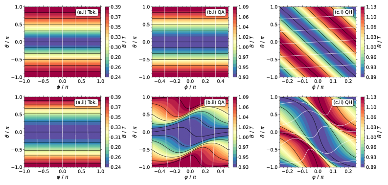
Figure 1: The magnetic field strength is plotted on the $\psi/\psi_{\mathrm{edge}}=0.5$ flux surface as a function of symmetry and geometric coordinates in the top and bottom rows, respectively. Each column, from left to right, corresponds to a circular tokamak, a precise QA, and a precise QH configuration, respectively. Included in each panel are the $\eta$ (black) and $\xi$ (white) contours. This shows that while the symmetry-aligned contours are uniformly distributed and orthogonal in symmetry coordinates, they are neither in geometric coordinates. Moreover, significant geometric deformations are observed in the non-axisymmetric configurations.

In Fig. 1, this is demonstrated for a tokamak with a circular cross-section and the precise QA and QH stellarators of Ref. Landreman and Paul (2022). In each panel, the magnetic field strength on the $\psi/\psi_{\mathrm{edge}}=0.5$ flux surface is shown, where, $\psi$ is the toroidal magnetic flux used to label each flux surface and $\psi_{\mathrm{edge}}$ is $\psi$ at the plasma boundary. Each flux surface is plotted over a single field period, and each column, respectively from left to right, corresponds to the tokamak, the precise QA, and the precise QH configuration. The top row shows $B$ as a function of $\theta$ and $\phi$. Contours of the symmetry angle $\eta$ are shown as black lines while contours of the cross-symmetry angle $\xi$ are shown as white lines. From these contours, the alignment of $\eta$ with the $B$ contours, as well as the quasi-orthogonality of $\xi$ and $\eta$ can be readily observed. Note that in the precise QH configuration shown in panel (c.i), the angle between the $\eta$ and $\xi$ contours appears larger than 90 degrees because of the aspect ratio between the poloidal and toroidal domains.

This quasi-orthogonality is only observed when the contours of $\eta$ and $\xi$ are represented in Boozer coordinates; in physical space, the coordinates are not in fact orthogonal. This is demonstrated in the bottom row of Fig. 1, where the same data is shown with respect to the geometric poloidal $\vartheta$ and geometric toroidal $\varphi$ coordinates. Importantly, these geometric coordinates define an orthogonal reference frame, so that curves that are orthogonal in this reference frame are orthogonal in physical space. Therefore, in this representation, it can be observed that the $\eta$ and $\xi$ contours are orthogonal in the axisymmetric tokamak, of panel (a.ii), but not in the non-axisymmetric QA and QH equilibria of panels (b.ii) and (c.ii), respectively. Moreover, panels (b.ii) and (c.ii) demonstrate the extent to which the symmetry-aligned contours are distorted in physical space for non-axisymmetric equilibria. The guiding assumption for defining the salient cross-sections is then that the geometric deformation of the symmetry-aligned contours contains important information on how the geometry of a flux surface relates to symmetries in $B$ on that surface.

To define a method for identifying salient cross-sections, consider first that the minor radius vector $\bm{\rho}$ of any cross-section can be defined as

$$\bm{\rho}(z,\,\lambda)=\mathbf{r}_{\mathrm{cs}}(z,\,\lambda)-\mathbf{r}_{\mathrm{ma}}(z),$$ (3)

where $z$ is a periodic coordinate along the magnetic axis that uniquely labels each cross-section and $\lambda$ is periodic coordinate along each cross-section. Furthermore, $\mathbf{r}_{\mathrm{ma}}$ is the vector that traces out the magnetic axis while $\mathbf{r}_{\mathrm{cs}}$ is a vector that traces out each cross-section path. Equation (3) is assumed to apply over a given flux surface, so any dependence on $\psi$ can be ignored.

The two cross-section criteria can be satisfied in an axisymmetric or a non-axisymmetric QA equilibrium by defining $\mathbf{r}_{\mathrm{cs}}$ as the $\xi$ contours (i.e. the white contours in Fig. 1). In the example of the QH $M=1$ and $N=-4$ equilibrium, however, the $\xi$ contours only close on themselves after four toroidal transits. Therefore, defining a cross-section in this way does not generalize to a QH equilibrium.

For an alternative method, consider the vector $\mathbf{r}_{\eta}=\mathbf{r}_{\eta}(\xi)$, which traces out a particular symmetry-angle contour of constant $\eta$. An additional vector $\mathbf{r}_{\mathrm{ax}}=\mathbf{r}_{\mathrm{ma}}-\mathbf{r}_{\eta}$ can then be defined that points from any point along $\mathbf{r}_{\eta}$ to a point along the magnetic axis. A flux-surface cross-section, uniquely labeled by $z$, can then be defined as the set of points that minimizes $r_{\mathrm{ax}}=\|\mathbf{r}_{\mathrm{ax}}\|$ along each $\mathbf{r}_{\eta}$ contour for a particular value of $z$, where $\|\cdot\|$ represents the $2$-norm. In this way, each cross-section is comprised of the points of closest approach of all symmetry-angle contours to that particular value of $z$ on the magnetic axis.

To prove that this definition satisfies the condition that one recovers a poloidal cross-section in an axisymmetric system, it is informative to first consider that

$$r_{\mathrm{ax}}=\left[\left(\mathbf{r}_{\mathrm{ma}}-\mathbf{r}_{\eta}\right)\cdot\left(\mathbf{r}_{\mathrm{ma}}-\mathbf{r}_{\eta}\right)\right]^{1/2}.$$

Therefore, any minimum of $r_{\mathrm{ax}}$ must satisfy the condition

$$\frac{\partial r_{\mathrm{ax}}}{\partial\xi}=-\frac{\mathbf{e}_{\xi}\cdot\mathbf{r}_{\mathrm{ax}}}{r_{\mathrm{ax}}}=0,$$ (4)

where $\partial\mathbf{r}_{\mathrm{ma}}/\partial\xi=0$ and $\mathbf{e}_{\xi}=\partial\mathbf{r}_{\eta}/\partial\xi$ is the covariant $\xi$ basis vector, which is tangent to $\mathbf{r}_{\eta}$. This means that a minimum in $r_{\mathrm{ax}}$ can only occur when a vector, tangent to a symmetry-angle contour, is orthogonal to the vector that points from that point to $\mathbf{r}_{\mathrm{ma}}(z)$. Immediately, one can infer that in an axisymmetric system, where $\xi=\varphi$ and $\mathbf{e}_{\xi}=\mathbf{e}_{\varphi}$, orthogonality between $\mathbf{r}_{\mathrm{ax}}$ and $\mathbf{e}_{\xi}$ means that $\mathbf{r}_{\mathrm{ax}}$ must lie within the plane perpendicular to the toroidal direction (i.e. a polodial cross-section).

Equation (4), however, is only sufficient to prove that $r_{\mathrm{ax}}$ is at a local extremum. A local minimum also requires that $\partial^{2}r_{\mathrm{ax}}/\partial\xi^{2}>0$. Therefore, taking a second derivative of Eq. (4), one finds

$$\frac{\partial^{2}r_{\mathrm{ax}}}{\partial\xi^{2}}=\frac{1}{r_{\mathrm{ax}}}\left[g_{\xi\xi}-\frac{\partial\mathbf{e}_{\xi}}{\partial\xi}\cdot\left(\mathbf{r}_{\mathrm{ma}}-\mathbf{r}_{\eta}\right)\right],$$ (5)

where $g_{\xi\xi}=\mathbf{e}_{\xi}\cdot\mathbf{e}_{\xi}$. To then derive an expression for $\partial\mathbf{e}_{\xi}/\partial\xi$, consider that in a Frenet-Serret frame D’haeseleer et al. (1991)

$$\frac{\partial^{2}\mathbf{r}_{\eta}}{\partial s^{2}}=\kappa\hat{\mathbf{N}},$$ (6)

where $s$ is the arc-length along the $\mathbf{r}_{\eta}$ contour, $\kappa$ is the local curvature of that contour, and $\hat{\mathbf{N}}$ is the normal unit vector orthogonal to the symmetry-angle contour tangent-vector. Expressed in terms of $\xi$, Eq. (6) becomes

$$\frac{\partial^{2}\xi}{\partial s^{2}}\mathbf{e}_{\xi}+\frac{1}{g_{\xi\xi}}\frac{\partial\mathbf{e}_{\xi}}{\partial\xi}=\kappa\hat{\mathbf{N}},$$ (7)

using the relation $\partial\xi/\partial s=1/\sqrt{g_{\xi\xi}}$. Then, rearranging Eq. (7) to isolate $\partial\mathbf{e}_{\xi}/\partial\xi$ and substituting into Eq. (5), one finds

$$\frac{\partial^{2}r_{\mathrm{ax}}}{\partial\xi^{2}}=\frac{g_{\xi\xi}}{r_{\mathrm{ax}}}\left(1-\kappa r_{\mathrm{ax}}\hat{\mathbf{N}}\cdot\hat{\mathbf{r}}_{\mathrm{ax}}\right),$$ (8)

with $\hat{\mathbf{r}}_{\mathrm{ax}}=\mathbf{r}_{\mathrm{ax}}/r_{\mathrm{ax}}$ and $\mathbf{e}_{\xi}\cdot\mathbf{r}_{\mathrm{ax}}=0$, where the latter is required to be consistent with Eq. (4). In Eq. (8), $r_{\mathrm{ax}}$ is positive definite, $\kappa\geq 0$, and $\hat{\mathbf{N}}\cdot\hat{\mathbf{r}}_{\mathrm{ax}}\in[-1,\,1]$. Therefore, independent of the value of the scalar product, $\partial^{2}r_{\mathrm{ax}}/\partial\xi^{2}>0$ if

$$\kappa<\frac{1}{r_{\mathrm{ax}}}.$$ (9)

This means that, in an axisymmetric system, if a poloidal cross-section satisfies Eq. (9), then that cross-section is defined as the set of points that locally minimize the distance between each symmetry-angle contour and the corresponding point on the magnetic axis. Moreover, in a non-axisymmetric equilibrium, the set of points that simultaneously satisfy Eqs. (4) and (9) describe a cross-section analogous to a poloidal cross-section in an axisymmetric configuration.

To determine whether a set of points satisfies these conditions, one can compute them both explicitly. However, if one considers that the $\mathbf{r}_{\eta}$ contour tends to wrap toroidally around a flux surface, then it can be argued that $\kappa\approx 1/R_{0}$, where $R_{0}$ is the major radius. If one then restricts ones analysis to only the set of points satisfying Eq. (4) that are in the vicinity of the specified axial position $z$, then $r_{\mathrm{ax}}\approx a$, where $a$ is the minor radius. From these scaling relations, Eq. (9) can be approximated as $a/R_{0}<1$, which is always observed. Therefore, the set of points satisfying Eq. (4) can be reasonably assumed to be a local minimum, provided they are points within the toroidal vicinity of $z$.

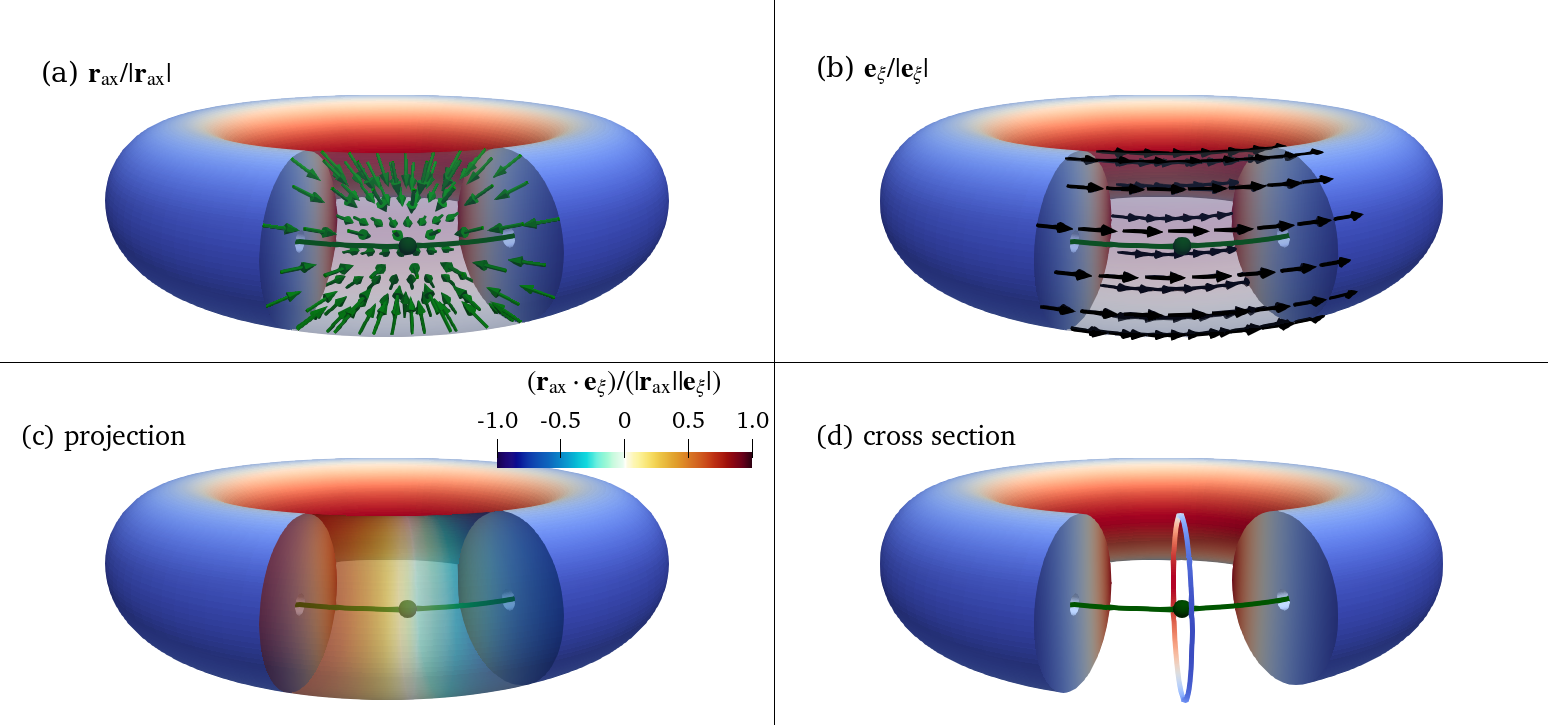
Figure 2: The algorithm for identifying a symmetry-defined cross-section is shown graphically in an axisymmetric configuration. Panel (a) shows the $\mathbf{r}_{\mathrm{ax}}$ vector field over a portion of a flux surface. Panel (b) shows the symmetry-aligned basis vector field $\mathbf{e}_{\xi}$ over the same domain. Then, panel (c) shows the projection of these two fields over that domain. Lastly, panel (d) shows the cross-section described by the roots of the projection. In each panel, the magnetic axis is shown as a green curve, while the point along the magnetic axis where the cross-section is defined is indicated with a green sphere.

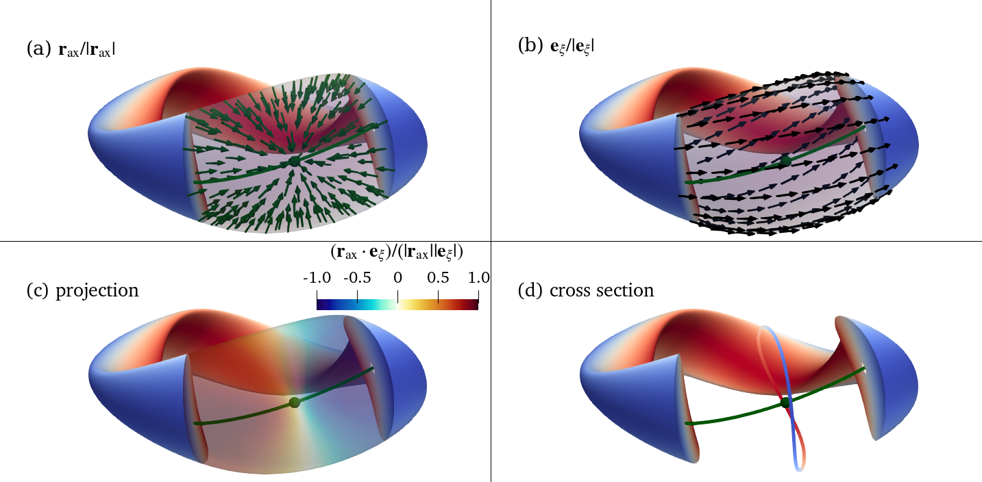
Figure 3: The algorithm for identifying a symmetry-defined cross-section is shown graphically in the precise QA configuration. Panel (a) shows the $\mathbf{r}_{\mathrm{ax}}$ vector field over a portion of a flux surface. Panel (b) shows the symmetry-aligned basis vector field $\mathbf{e}_{\xi}$ over the same domain. Then, panel (c) shows the projection of these two fields over that domain. Lastly, panel (d) shows the cross-section described by the roots of the projection. In each panel, the magnetic axis is shown as a green curve, while the point along the magnetic axis where the cross-section is defined is indicated with a green sphere.

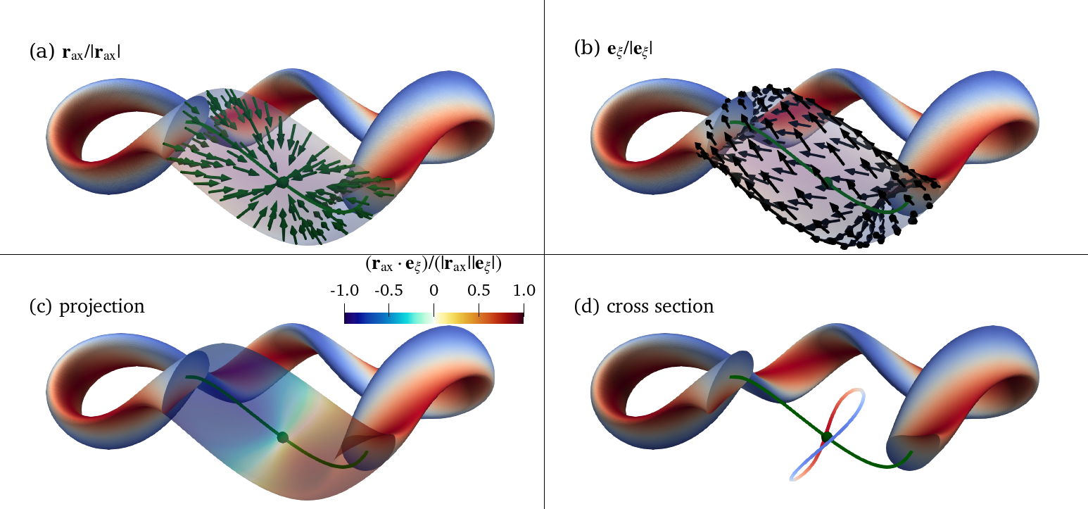
Figure 4: The algorithm for identifying a symmetry-defined cross-section is shown graphically in the precise QH configuration. Panel (a) shows the $\mathbf{r}_{\mathrm{ax}}$ vector field over a portion of a flux surface. Panel (b) shows the symmetry-aligned basis vector field $\mathbf{e}_{\xi}$ over the same domain. Then, panel (c) shows the projection of these two fields over that domain. Lastly, panel (d) shows the cross-section described by the roots of the projection. In each panel, the magnetic axis is shown as a green curve, while the point along the magnetic axis where the cross-section is defined is indicated with a green sphere.

For the cross-sections considered in this paper, the toroidal vicinity is taken to mean a set of points along a flux surface within a half-field-period on either side of some position $z$. To compute the related cross-section, one first computes the $\mathbf{r}_{\mathrm{ax}}$ and $\mathbf{e}_{\xi}$ vector fields over that domain. Then, a root-finding algorithm can be used to find the set of points along the flux surface that satisfy the relation $\mathbf{r}_{\mathrm{ax}}\cdot\mathbf{e}_{\xi}=0$. Three such example calculations are shown in Figs. 2–4, which correspond to the tokamak, the precise QA, and the precise QH configurations, respectively. In each figure, the magnetic axis is represented as a green curve with the specified $z$ position shown with a green sphere. The $\mathbf{r}_{\mathrm{ax}}$ field is shown in panel (a), the $\mathbf{e}_{\xi}$ field is shown in panel (b), the scalar projection between the two fields is shown in panel (c), and the resulting cross-section is shown in panel (d).

From these figures, it can be observed that the resulting cross-section in the tokamak is a poloidal cross-section, as is expected. In the non-axisymmetric equilibria, the analogous cross-sections are non-planar. This is due to the variation in the direction of $\mathbf{e}_{\xi}$ over their flux surface, resulting in a torsioning of the curve that connects the set of points satisfying Eq. (4). The assumption is then that the poloidal cross-section is useful for categorizing the various shapes achieved in axisymmetric equilibria, and that the analagous non-axisymmetric cross-sections can be used for similar purposes.

II.1 Defining equilibrium shapes via modal analysis

In either axisymmetric or non-axisymmetric equilibria, the set of cross-sections can be represented as $\bm{\rho}(z,\eta)=\rho\hat{\bm{\rho}}$, where $\eta$ plays the role of $\lambda$ in Eq. (3). The cross-section path $\hat{\bm{\rho}}(z,\eta)$ is a unit vector that points from the $z$ point on magnetic axis to the corresponding cross-section. Then, the minor radius $\rho(z,\eta)$ is the distance from the axis to the cross-section. In an axisymmetric cross-section, notions of shaping (i.e. elongation, triangularity, squareness, etc.) are defined exclusively by the minor radius $\rho$. This equivalently applies to shapes defined by $\rho$ in non-axisymmetric equilibria.

To define the generalized set of equilibrium shapes, the minor radius is expanded with a cosine basis as

$$\rho(z,\eta)=\rho_{\mathrm{eff}}(z)\left[1+\sum\limits_{\ell=1}^{\infty}\rho_{\ell}(z)\cos(\ell\eta)\right],$$ (10)

though in practice this sum can often be truncated to $\ell\lesssim 10$. This defines a modal representation for the minor radius of each cross-section. In this representation, $\rho_{\mathrm{eff}}$ is the effective minor radius of a circular cross-section. Each shaping mode amplitude $\rho_{\ell}$ describes some additional shaping of that cross-section with respect to changes in the symmetry-aligned coordinate $\eta$.

Figure 5: The $\ell=1,\,2,\ 3,$ and $4$ shaping modes are shown for how they weight different segments of a cross-section in panels (a), (b), (c), and (d), respectively. Cross-section segments weighted positively are are shown in red while segments weighted negatively are shown in blue. The magnitude of the weights is represented by the distance of each curve from the magnetic axis, located at $(0,\ 0)$ and the blue/red shading. This provides a pictorial interpretation of how the shaping modes relate to familiar concepts like the Shafranov shift and shaping parameters like elongation, triangularity, and squareness.

To best interpret the modal amplitudes, consider that the low-field side of each cross-section corresponds to $\eta=0$ while the high-field side corresponds to $\eta=\pi$. Figure 5 then shows how each $\cos(\ell\eta)$ mode weights different segments of a cross-section’s minor radius for values of $\ell=1,\ 2,\ 3,$ and $4$ in panels (a), (b), (c), and (d), respectively. Note that positive values of $\cos(\ell\eta)$ are shown in red and negative values in blue, while the magnitude of $\cos(\ell\eta)$ is depicted as both the distance from the origin—the magnetic axis—and the red/blue shading. From panel (a), $\rho_{\ell}$ can be related to a Shafranov-like shift, though its more precise interpretation is as a measure of the translation of the magnetic axis relative to the geometric center along an axis that connects the low- and high-field side of a cross-section. This can be understood by considering a circular cross-section whose magnetic axis is shifted towards the low-field side. The $\ell=1$ mode of such a cross-section will provide more negative (i.e. blue) than positive (i.e. red) weighting, resulting in $\rho_{\ell}<0$. Conversely, if the magnetic axis is shifted towards the high-field side, then $\rho_{\ell}>0$.

Similarly, from panel (b), a cross-section that is elongated along the axis that connects the low- and high-field sides will result in $\rho_{2}>0$, while a cross-section elongated in the direction perpendicular to that will result in $\rho_{2}<0$. In an axisymmetric cross-section, these values of $\rho_{2}$ correspond to a horizontal and vertical elongation, respectively. Continuing in this manner, from panel (c) a positive value of $\rho_{3}$ can be interpreted as exhibiting positive triangularity while a negative value describes negative triangularity. Similarly, panel (d) shows that a positive value of $\rho_{4}$ describes a diamond-shaped cross-section while a negative value describes a square-shaped cross-section. This method of interpreting the shaping mode amplitudes extends to any arbitrary order in $\ell$.

After one computes the set of cross-sections for a given equilibrium using the method described in Sec. II, the shaping mode amplitudes can then be computed as

$$\rho_{\ell}(z)=\frac{1}{\rho_{\mathrm{eff}}}\int\limits_{0}^{2\pi}\rho(z,\,\eta)\cos(\ell\eta)d\eta,$$ (11)

with $\ell$ being any positive integer and

$$\rho_{\mathrm{eff}}(z)=\int\limits_{0}^{2\pi}\rho(z,\,\eta)d\eta.$$ (12)

In this way, $\rho_{\ell}$ describes a discrete shaping spectrum that can be used to interpret equilibrium shapes in both axisymmetric and non-axisymmetric geometries, with the only difference being that in non-axisymmetric equilibria $\rho_{\ell}$ is a function of $z$. This dependence on $z$ will be discussed further in the proceeding section.

III Shaping Analysis in Non-axisymmetric Equilibria

In this section, the novel shaping method is used to analyze the shape of the precise quasi-symmetric configurations from Ref. Landreman and Paul (2022). To compute these and all other equilibria in this paper, the Variational Moment Equilibrium Code (VMEC) Hirshman and Whitson (1983) is used. VMEC is run in fixed-boundary mode with the pressure and current profiles assumed to be zero, resulting in the vacuum-field configurations.

In order to treat the axial dependence of $\rho_{\ell}$, it is desirable to choose a value for $z$ that is consistent with the symmetry-aligned coordinates $(\eta,\ \xi)$ used to define each cross-section. The symmetry-aligned coordinates, however, are simply the linearly shifted Boozer coordinates $(\theta,\ \phi)$, as defined in Eqs. (1) and (2). Therefore, it is sufficient to let $z=\phi_{\mathrm{ma}}$, where $\phi_{\mathrm{ma}}$ is $\phi$ along the magnetic axis.

Notably, from a VMEC equilibrium, one is able to compute the transform from VMEC to Boozer coordinates. However, this transformation is not defined on the magnetic axis, meaning one cannot compute $\phi_{\mathrm{ma}}$. Alternatively, an intermediate set of straight-field-line coordinates called PEST coordinates are defined along the magnetic axis boo , but using these PEST coordinates to compute the symmetry-aligned coordinates results in a systematic error. This is because the resulting $\eta$ and $\xi$ contours are not perfectly aligned with the idealized symmetry and cross-symmetry directions. This error, however, can be quantified, and one may choose to consider only configurations with a tolerably low error. For details on this error quantification, see Appendix B. In the remainder of this paper, it should be understood that $\phi_{\mathrm{ma}}$ and the corresponding cross-sections are computed in PEST coordinates.

To better account for the $\phi_{\mathrm{ma}}$ dependence of $\rho_{\ell}$ in a non-axisymmetric configuration, consider that $\rho_{\ell}$ is periodic in $\phi_{\mathrm{ma}}$, with that periodicity defined as $\rho_{\ell}(\phi_{\mathrm{ma}})=\rho_{\ell}(\phi_{\mathrm{ma}}+2\pi/n_{\mathrm{fp}})$, and $n_{\mathrm{fp}}$ the number of field periods. This allows one to take a discrete Fourier transform of $\rho_{\ell}$, resulting in a Fourier-transformed shaping spectrum (FTSS). This FTSS is represented as $\hat{\rho}_{\ell}(k_{\phi})$, where $k_{\phi}$ is a toroidal wavenumber that is a whole number multiple of $n_{\mathrm{fp}}$. In an axisymmetric equilibrium, the FTSS results in shaping modes with $k_{\phi}=0$, meaning the corresponding shapes undergo no rotation as one traverses the magnetic axis. Alternatively, in a non-axisymmetric equilibrium, a $\hat{\rho}_{2}$ shaping mode with $k_{\phi}=n_{\mathrm{fp}}$ can be readily interpreted as an elongated shape that undergoes a $\pi$ rotation about the magnetic axis once per field period. If $k_{\phi}=2n_{\mathrm{fp}}$, the elongated shape rotates $2\pi$ per field period. Similar interpretations exist for all $\hat{\rho}_{\ell}$ and any integer value of $k_{\phi}/n_{\mathrm{fp}}$.

With that taken into consideration, this section investigates the shaping spectra and the FTSS of both the precise QA and QH configurations and their corresponding initialization configurations from which they were optimized. From this analysis, it is shown that the FTSS provides a low-order shaping representation while also revealing a regularized spatial structure that emerges in both optimized quasi-symmetric configurations. This provides the first evidence that the cross-sections, defined in Sec. II, contain important information regarding the relationship between flux-surface geometry and quasi-symmetry.

III.1 Precise QA

Figure 6: The initial (a) and optimized (b) cross-sections are shown over a half-field-period for the QA configuration of Ref. Landreman and Paul (2022). These cross-sections are continuous across $\psi/\psi_{\mathrm{edge}}\in[0.005,\,1]$. The corresponding shaping spectra in Fig. 7 are computed on the $\psi/\psi_{\mathrm{edge}}=0.5$ flux surface, which is shown here on each cross-section as a black curve.

The first configurations to be considered are the precise QA and its initialization configuration, the latter of which is an axisymmetric configuration with a circular cross-section. The cross-sections for both configurations are shown over a half-field-period in Fig. 6, with the initial configuration shown in panel (a) and the optimized configuration in panel (b). Note that the cross-sections are plotted across radial positions $0.005\leq\psi/\psi_{\mathrm{edge}}\leq 1$, but the subsequent analysis is performed only for the $\psi/\psi_{\mathrm{edge}}=0.5$ flux surface, which is indicated along each cross-section with a black curve. Repeating the analysis over different radial positions does not significantly impact the results. In this section, all cross-sections are computed with $\eta$ defined in PEST coordinates and $M=1$ and $N=0$ symmetry.

Figure 7: A comparative shaping analysis between the initial and optimized QA configurations, with the initial configuration shown in the top row and the optimized configuration in the bottom row. The left column shows the corresponding shaping spectrogram on a linear color scale and the right column shows the amplitudes of the FTSS on a logarithmic color scale. Included in panel (d) is a dashed black line with a slope of 3/1, showing how the shaping modes are distributed in the FTSS of the optimized QA. This figure shows how the equilibrium shape changed over the course of the optimization to produce a precise QA equilibrium.

Figure 7 shows the shaping spectra and FTSS amplitudes for both the initial and optimized QA. The shaping data for the initial configuration are shown on the top row and the optimized configuration on the bottom row. The left column shows the toroidally-dependent shaping spectra while the right column shows the $k_{\phi}$-dependent amplitudes of the FTSS. The independent $\phi_{\mathrm{ma}}$ and $k_{\phi}$ variables are plotted along the horizontal axis, while the shaping mode index $\ell$ is plotted along the vertical axis. The values of both $\rho_{\ell}(\phi_{\mathrm{ma}})$ and $|\hat{\rho}_{\ell}(k_{\phi})|$ are represented by their respective color scales. Note that $|\hat{\rho}_{\ell}(k_{\phi})|$ is shown on a logarithmic color scale that spans four orders of magnitude.

As expected from the circular cross-sections observed in Fig. 6(a), the $\rho_{\ell}$ shaping mode dominates the shaping spectrum of the initial configuration, with its positive value indicating that the magnetic axis is shifted towards the high-field side of the torus relative to the geometric center. Moreover, the constancy of $\rho_{\ell}$ across the $\phi_{\mathrm{ma}}$ domain, as observed in panel (a), shows this shift does not depend on the axial position. This leads to $k_{\phi}=0$ for all shaping modes in the corresponding FTSS shown in panel (b).

Comparatively, the optimized QA configuration exhibits significantly more shaping, with shaping modes for $\ell\leq 6$ shown on the linear scaling of panel (c) and shaping modes for $\ell\leq 12$ on the logarithmic scale of panel (d). Clear trends can be observed. First, from both panels (c) and (d), the $\rho_{2}$ shaping mode is seen to provide the largest amplitude contribution to the shaping spectrum, while panel (d) further shows that the elongated shape undergoes a $\pi$ rotation once per field period. This is an intuitive result, considering the visibly elongated cross-sections in Fig. 6(b) can be observed to rotate by $\pi/2$ over a single half-field period. Surprisingly, however, the FTSS shown in panel (d) reveals that as shaping modes increase in $\ell$, those modes are observed to rotate increasingly quickly about the magnetic axis, as reflected in a proportional increase in their $k_{\phi}$. To highlight this trend, a dashed black line with a slope of 3/1 is included in panel (d), centered on the $\ell=2$ and $k_{\phi}/n_{\mathrm{fp}}=1$ cell. It can be observed that the large-amplitude shaping modes are clustered around this line. The presence of such a distribution trend of shaping modes implies that a kind of spatial resonance between shape complexity and axial rotation has emerged over the course of the optimization.

III.2 Precise QH

Figure 8: The initial (a) and optimized (b) cross-sections are shown over a half-field-period for the QH configuration of Ref. Landreman and Paul (2022). These cross-sections are continuous across $\psi/\psi_{\mathrm{edge}}\in[0.005,\,1]$. The corresponding shaping spectra in Fig. 9 are computed on the $\psi/\psi_{\mathrm{edge}}=0.5$ flux surface, which is shown on each cross-section as the black curve.

Next, the precise QH configuration is analyzed, with the corresponding figures organized identically to those in the preceding section. Figure 8 shows the initial (a) and optimized (b) cross-sections across all $0.005\leq\psi/\psi_{\mathrm{edge}}\leq 1$ flux surfaces, with the magnetic axis shown as a green curve. All shaping analysis is performed on the $\psi/\psi_{\mathrm{edge}}=0.5$ flux surface, which is indicated with the black line along each cross-section. All cross-sections are computed with $\eta$ defined in PEST coordinates and $M=1$ and $N=-4$ symmetry. Similar to Fig. 6(a), the initial QH spectrogram is comprised of planar cross-sections that are perpendicular to the magnetic axis, while the optimized configuration produces torsioned cross-sections.

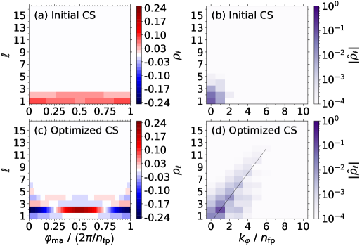
Figure 9: A comparative shaping analysis between the initial and optimized QH configurations, with the initial configuration shown in the top row and the optimized configuration in the bottom row. The left column shows the corresponding shaping spectrogram on a linear color scale and the right column shows the amplitudes of the FTSS on a logarithmic color scale. Included in panel (d) is a dashed black line with a slope of 2/1, showing how the shaping modes are distributed in the FTSS of the optimized QH. This figure shows how the equilibrium shape changed over the course of the optimization to produce a precise QH equilibrium.

Figure 9 shows a shaping analysis comparison between the initial and optimized QH configurations. From panels (a) and (b), the shaping modes of the planar cross-sections in the initial configuration are observed to exhibit some toroidal dependence. This indicates that the position of these cross-sections relative to the magnetic axis changes over a field period. Similar to what is observed for the precise QA, the optimized QH shaping is dominated by the $\ell=2$ mode undergoing a $\pi$ rotation once per field period, which is also consistent with the cross-sections shown in Fig. 8(b), where the visibly elongated axis of each cross-section is observed to undergo a $\pi/2$ rotation over a half-field period. Then, starting from the $\ell=2$ and $k_{\phi}=1$ mode in the FTSS of panel (d), the dominant shaping modes are distributed about a straight line with a slope of $2/1$, with the FTSS amplitudes quickly decaying to values that likely fall below the error threshold. The observation of a shape scaling in the precise QH configuration is consistent with the analogous observation in Fig. 7(d) for the precise QA. This bolsters the claim that quasi-symmetry results from a resonance that requires increasingly higher-order shaping modes to rotate more quickly about the magentic axis. In the next section, this and other trends are investigated in the QUASR database.

IV Shaping Across the QUASR Database

The QUASR database provides over $3.7\times 10^{5}$ stellarator geometries, with approximately 54% of them QA and the remaining QH Giuliani (2024). Therefore, this database provides a useful dataset with which the stellarator shaping trends identified in Sec. III can be investigated. The present investigation does not utilize the entire database. Instead, the FTSS is presented for a sample of configurations from throughout the database. This is sufficient, however, to provide novel insights into how the FTSS reveals trends in stellarator shaping as it relates to quasi-symmetry and other macroscopic properties.

The primary reason for the reduced sampling is that approximately 30% of the database failed to converge to a solution in VMEC. The reason for this is likely due to the large peak torsion in the magnetic axis of the failed configurations. This is a problem for VMEC because the code uses a cylindrical coordinate system for its real-space map, which is not a coordinate system well suited for configurations in which the magnetic axis is significantly displaced from the azimuthal plane. Other ideal-MHD equilibrium codes like DESC Dudt and Kolemen (2020) or GVEC Hindenlang et al. (2025) may have a higher success rate for generating these highly torsioned equilibria. Moreover, these other equilibrium codes allow for a transformation to Boozer coordinates along the magnetic axis, allowing for a more accurate computation of each equilibrium’s FTSS. For this reason, a more analytic and statistically robust investigation of equilibrium shapes in the QUASR database is left for a future work. The present analysis is instead focused on the subset of converged VMEC equilibria.

Most of the highly torsioned configurations that are excluded are QH equilibria with $n_{\mathrm{fp}}\geq 6$. Also, no $n_{\mathrm{fp}}=1$ QH equilibria are found in the database. Therefore, to compare the influence of shaping in both QA and QH configurations, the shaping analysis performed is restricted to configurations with $2\leq n_{\mathrm{fp}}\leq 5$. QA configurations are considered in Sec. IV.1 and QH configurations in Sec. IV.2. In both cases, the FTSS of 21 individual configurations reveal salient shaping trends in relation to the quasi-symmetry, number of field periods, and rotational transform of the equilibria. To provide evidence of these trends from across the database, FTSS histograms are introduced that depend on $\ell$ and a weighted average of $k_{\phi}$.

For a given $\ell$, the weighted average of $k_{\phi}$ is defined as

$$\bar{k}_{\phi}(\ell)=\frac{n_{\mathrm{fp}}\sum\limits_{i=0}^{20}i|\hat{\rho}_{\ell}(in_{\mathrm{fp}})|}{\sum\limits_{i=0}^{20}|\hat{\rho}_{\ell}(in_{\mathrm{fp}})|}.$$

It is found that $\bar{k}_{\phi}/n_{\mathrm{fp}}$ is converged to variations well below unity when the summation is truncated to $k_{\phi}/n_{\mathrm{fp}}\leq 20$. Additionally, the quasi-symmetry is quantified by computing the root-sum-square of the symmetry breaking modes in the Boozer spectrum, defined as

$$\mathcal{Q}_{\mathrm{err}}=\frac{1}{B_{0,0}}\left(\sum\limits_{\begin{subarray}{c}n\neq iN\\ m\neq iM\end{subarray}}B^{2}_{n,m}\right)^{1/2}.$$

Here, $n$ and $m$ are the toroidal and poloidal mode numbers, $B_{n,m}$ the corresponding Boozer mode amplitudes, $B_{0,0}$ is the flux-surface-averaged magnetic field strength, and $i$ is any whole number.

IV.1 Quasi-axisymmetry in QUASR Database

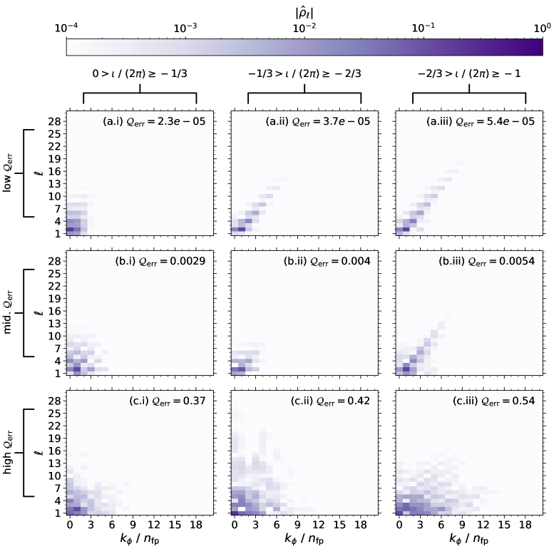
Figure 10: The FTSS is shown for 9 QA configurations from the QUASR database. The configurations are ordered by the absolute value of their rotational transform, which increases from the left (i) to the right (iii) column, and the quasi-symmetry error, which increases from the top (a) to the bottom (c) row. This ordering is further characterized by the annotations for the rotational transform and the quasi-symmetry error at the top and left side of the figure, respectively. The quasi-symmetry error of each configuration is recorded at the top right of each panel. These FTSS provide support for the claim that quasi-symmetry results from a resonance between shape complexity and axial rotation.

Figure 10 shows the FTSS for 9 configurations sampled from the set of QA configurations. These configurations are sampled without any regard to their number of field periods. The configurations are organized by their rotational transform and quasi-symmetry error $\mathcal{Q}_{\mathrm{err}}$. The rows are labeled from (a)–(c) going from the top to the bottom, with configurations ordered by increasing $\mathcal{Q}_{\mathrm{err}}$, as indicated by the annotations on the left side of the figure. From row (a) to (c), $\mathcal{Q}_{\mathrm{err}}$ increases by approximately four orders of magnitude, from $\mathcal{Q}_{\mathrm{err}}\approx 10^{-5}$ to $10^{-1}$. The $\mathcal{Q}_{\mathrm{err}}$ for each individual configuration is shown in the top right of each panel. The columns are labeled from (i)–(iii) going from left to right, with increasing absolute value of the rotational transform. These changes are also annotated for each column at the top of the figure, showing that $\iota$ spans $[-1,0]$ in three steps of $1/3$ width.

From this figure, multiple important trends can be observed. First, along row (a), where one finds the configurations with the smallest quasi-symmetry error, the largest-amplitude shaping modes in the FTSS tend to be distributed around a particular line, while the slope of this line decreases with increasing $|\text{\sout{$\iota$}}|$. As one moves down a column, the amplitudes of the shaping modes distributed further away from this line increase with the quasi-symmetry error. Additionally, in configurations with relatively low quasi-symmetry error (i.e., row (a)), the shaping-mode amplitudes extend further along the line with increasing $|\text{\sout{$\iota$}}|$. For configurations with relatively large quasi-symmetry error (i.e., rows (c)), an increase in the absolute value of the rotational transform is correlated with an increase in the shaping amplitudes with $\ell\lesssim 10$ and increasing toroidal rotation.

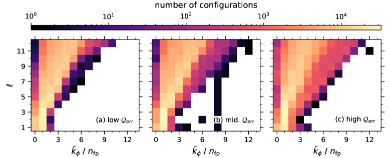
Figure 11: Three FTSS histograms are shown for the QA configurations in the QUASR database. The numerical bounds for the (a) low $\mathcal{Q}_{\mathrm{err}}$, (b) middle $\mathcal{Q}_{\mathrm{err}}$, and (c) high $\mathcal{Q}_{\mathrm{err}}$ subsets are provided in the text. The histograms show the number of configurations that have the specified weighted average of $k_{\phi}$ for a given $\ell$. These data show that quasi-symmetry is deteriorated when shaping modes rotate too quickly or too slowly about the magnetic axis.

To investigate the relationship between a linear shape distribution and the quality of quasi-symmetry, three FTSS histograms are shown in Fig. 11. These histograms are constructed by partitioning all the QA configurations into three subsets with an equal number of configurations but of varying quasi-symmetry quality. In all three subsets, the weighted averaged of $k_{\phi}$ is computed for $\ell\leq 12$ across all configurations. The color scale shows the number of configurations within each subset that have a particular $\bar{k}_{\phi}$ at a given $\ell$. The histogram in panel (a) shows the low $\mathcal{Q}_{\mathrm{err}}$ configurations with $2.3\times 10^{-5}\leq\mathcal{Q}_{\mathrm{err}}<6.4\times 10^{-4}$, in panel (b) are the middle $\mathcal{Q}_{\mathrm{err}}$ configurations with $6.4\times 10^{-4}\leq\mathcal{Q}_{\mathrm{err}}<5.9\times 10^{-3}$, and in panel (c) are the high $\mathcal{Q}_{\mathrm{err}}$ configurations with $5.9\times 10^{-3}\leq\mathcal{Q}_{\mathrm{err}}<0.55$.

From these data, one can observe that the $\bar{k}_{\phi}$ width in panel (a) is peaked around a group of linear distributions, forming a cone of bright orange to yellow cells. As $\mathcal{Q}_{\mathrm{err}}$ increases in the transition to panels (b) and (c), this conic distribution is observed to broaden. The broadening is due to the inclusion of both fast and slow axial rotations of the shaping modes, leading to greater variability in the weighted average of $k_{\phi}$. Therefore, these data provide strong support for the claim that quasi-symmetry results from a resonance between shape complexity and axial rotation. Here, deviations from that resonance, with shapes rotating too quickly or too slowly, results in a deterioration in quasi-symmetry.

Moreover, the narrowing in the distribution of $\bar{k}_{\phi}$ in panel (a) relative to panels (b) and (c) shows that configurations with good quasi-symmetry exhibit fewer degrees of freedom in their shape description relative to configurations with poor quasi-symmetry. This demonstrates that the shaping method results in a reduced-order shape representation in a QA equilibrium. Therefore, this method can facilitate more systematic investigations into the effect of shaping on other figures of merit.

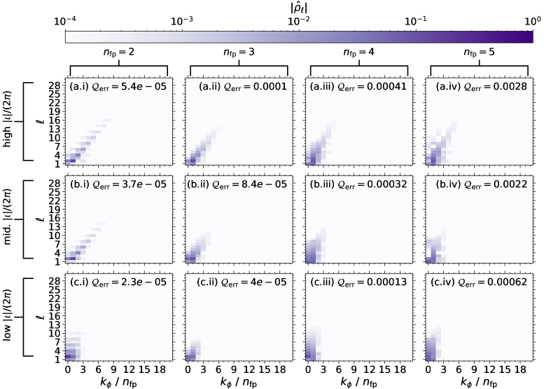
Figure 12: The FTSS is shown for 12 QA configurations from the QUASR database. The configurations are ordered by their number of field periods, which increases from the left (i) to the right (iv) column, and the absolute value of their rotational transform, which increases from the bottom (c) to the top (a) row. This ordering is further characterized by the annotations at the top and left side of the figure. The quasi-symmetry error of each configuration is recorded at the top right of each panel. These data demonstrate how the features of the linear shape distribution depends on both the rotational transform and the number of field periods, as described in the text.

To investigate the dependencies of a linear shape distribution in configurations with good quasi-symmetry, Fig. 12 shows the FTSS for a set of 12 QA configurations sampled from the set of low $\mathcal{Q}_{\mathrm{err}}$ configurations of Fig. 11(a). In Fig. 12, configurations increase in their number of field periods from the left to the right, with four columns spanning $n_{\mathrm{fp}}\in[2,5]$. From the bottom to the top row, configurations increase in the absolute value of their rotational transform, with low $|\text{\sout{$\iota$}}|$ configurations in row (c) constrained to $0>\text{\sout{$\iota$}}\geq-1/3$, the middle $|\text{\sout{$\iota$}}|$ configurations in row (b) constrained to $-1/3>\text{\sout{$\iota$}}\geq-2/3$, and the high $|\text{\sout{$\iota$}}|$ configurations in row (a) constrained to $-2/3>\text{\sout{$\iota$}}\geq-1$. The number of field periods is annotated at the top of each column and the $\iota$ constraint is annotated at the left of each row. Each panel shows the FTSS of the configuration with the lowest quasi-symmetry error from the set of configurations that adhere to the $\iota$ and $n_{\mathrm{fp}}$ values of the corresponding row and column, respectively. The quasi-symmetry error for each configuration is included in the top right of each panel.

Considering the influence of the rotational transform on each FTSS in Fig. 12, it can be inferred that if one aims to increase $|\text{\sout{$\iota$}}|$ while preserving the quasi-symmetry, it is necessary to do one of two things. First, one may reduce the slope of the line around which the shaping modes are distributed. This is observed in the transition from row (c) to (b) across all columns. Second, one may increase the higher-order shaping-mode amplitudes further along the distribution line—referred to as shape complexity—as can be seen in the transition from row (b) to (a). Ultimately, these observations suggest that the rotational transform, in a QA equilibrium, is related to the rate of increase of axial rotation with respect to progressively higher order shapes, and the shape complexity along this particular linear distribution.

Another observation can be made regarding the influence of the number of field periods. Namely, shape complexity is reduced in the transition from column (i) to (ii). This, however, does not result in a reduction in $|\text{\sout{$\iota$}}|$, which implies that increasing the number of field periods allows for a comparable rotational transform with less shape complexity. This trend is not observed in the subsequent transitions to $n_{\mathrm{fp}}=4$ and $5$ in columns (iii) and (iv), respectively. However, in these transitions, the quasi-symmetry error is observed to increase by one to two orders of magnitude relative to values in column (ii). This implies that the reduction in shape complexity that results from an increase in the number of field periods has a limit. Beyond this limit, increasing $n_{\mathrm{fp}}$ results in a deterioration in quasi-symmetry without any further reduction in shape complexity.

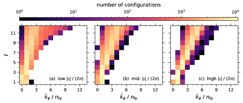
Figure 13: Three FTSS histograms are shown, comprised of QA configurations from the set of low $\mathcal{Q}_{\mathrm{err}}$ configurations in Fig. 11(a). The numerical bounds for the (a) low $|\text{\sout{$\iota$}}|$, (b) middle $|\text{\sout{$\iota$}}|$, and (c) high $|\text{\sout{$\iota$}}|$ subsets are provided in the text. The histograms show the number of configurations that have the specified weighted average of $k_{\phi}$ for a given $\ell$. These data indicate that in a QA stellarator, one can increase $|\text{\sout{$\iota$}}|$ by increasing the rate at which axial shape rotations increase with shape complexity.

Regarding the dependence of the rotational transform on the slope of a linear shape distribution, Fig. 13 shows three FTSS histograms. The configurations in these histograms are all selected from the set of low $\mathcal{Q}_{\mathrm{err}}$ configurations of Fig. 11(a), subdivided into three subsets with an equal number of configurations in each. The first low $|\text{\sout{$\iota$}}|$ subset, with $-0.09>|\text{\sout{$\iota$}}|\geq-0.20$, is shown in panel (a). The middle $|\text{\sout{$\iota$}}|$ subset, with $-0.20>|\text{\sout{$\iota$}}|\geq-0.40$, is shown in panel (b). The high $|\text{\sout{$\iota$}}|$ subset, with $-0.40>|\text{\sout{$\iota$}}|\geq-0.95$, is shown in panel (c).

From the low $|\text{\sout{$\iota$}}|$ histogram in panel (a), one can observe that the histogram peak occurs along a steeply sloped distribution line with a broad width in $\bar{k}_{\phi}$. This is observed in comparison to panel (b), in which the middle $|\text{\sout{$\iota$}}|$ histogram exhibits a narrowing in the $\bar{k}_{\phi}$ width and a decrease in the distribution slope of the histogram peak. This trend continues in the transition to the high $|\text{\sout{$\iota$}}|$ histogram in panel (c). In these latter configurations, the $\bar{k}_{\phi}$ width is further narrowed and the distribution slope of the histogram peak is minimized across all three histograms.

It is well established from the near-axis expansion of an ideal-MHD equilibrium that an elliptical plasma, rotating about the magnetic axis, can produce a rotational transform Helander (2014). It is therefore an intuitive result in the present context that an increase in the rotation of higher-order shaping modes (i.e., $\ell>2$) along a linear shape distribution is correlated with an increase in $|\text{\sout{$\iota$}}|$. Moreover, the fact that such an intuitive trend is revealed in the present shaping analysis demonstrates the utility of that shaping analysis in relating an equilibrium geometry to a figure of merit.

IV.2 Quasi-helical symmetry in QUASR Database

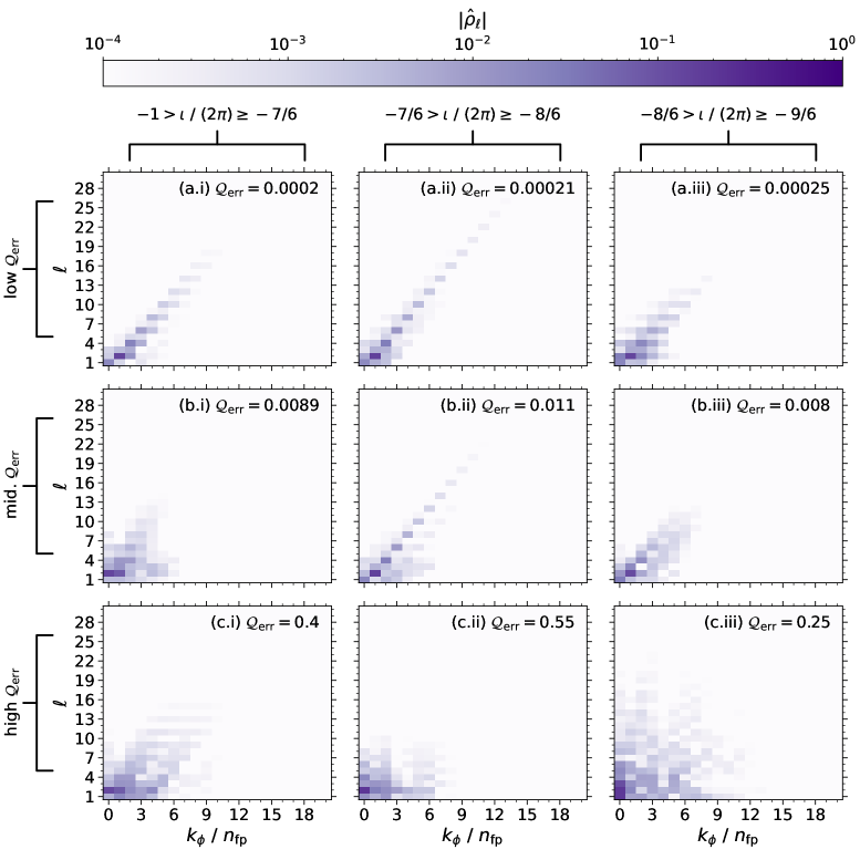
Figure 14: The FTSS is shown for 9 QH configurations from the QUASR database. The configurations are ordered by the absolute value of their rotational transform, which increases from the left (i) to the right (iii) column, and the quasi-symmetry error, which increases from the top (a) to the bottom (c) row. This ordering is further characterized by the annotations for the rotational transform and the quasi-symmetry error at the top and left side of the figure, respectively. The quasi-symmetry error of each configuration is recorded at the top right of each panel. These FTSS provide support for the claim that quasi-symmetry results from a resonance between shape complexity and axial rotation.

A similar analysis as was presented for QA equilibria is presented here for the set of QH equilibria. Figure 14 is analogous to Fig. 10 in that the FTSS for an array of 9 QH equilibria is presented with the absolute value of the rotational transform increasing from left to right along each row and the quasi-symmetry error increasing from top to bottom along each column. Importantly, a similar trend to that observed in the QA equilibria is observed for the QH equilibria. Namely, along each column, configurations with increasing quasi-symmetry error include larger-amplitude modes with no characteristic line distribution. This provides further support for the claim that quasi-symmetry results from a spatial resonance between shape complexity and axial rotation.

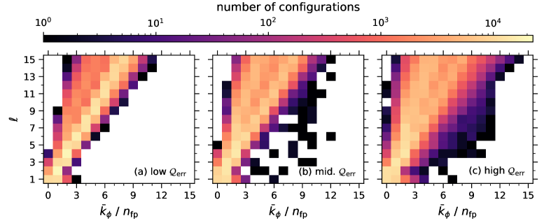
Figure 15: Three FTSS histograms are shown for the QH configurations in the QUASR database. The numerical bounds for the (a) low $\mathcal{Q}_{\mathrm{err}}$, (b) middle $\mathcal{Q}_{\mathrm{err}}$, and (c) high $\mathcal{Q}_{\mathrm{err}}$ subsets are provided in the text. The histograms show the number of configurations that have the specified weighted average of $k_{\phi}$ for a given $\ell$. These data show that quasi-symmetry is deteriorated when shaping modes rotate too quickly or too slowly about the magnetic axis.

Similar to Fig. 11 in Sec. IV.1, Fig. 15 shows three FTSS histograms constructed by partitioning the QH configurations into three subsets with an equal number of configurations and varying quasi-symmetry quality. The histogram in panel (a) shows the low $\mathcal{Q}_{\mathrm{err}}$ configurations with $2.0\times 10^{-4}\leq\mathcal{Q}_{\mathrm{err}}<1.5\times 10^{-3}$, in panel (b) the middle $\mathcal{Q}_{\mathrm{err}}$ configurations with $1.5\times 10^{-3}\leq\mathcal{Q}_{\mathrm{err}}<4.9\times 10^{-3}$, and in panel (c) the high $\mathcal{Q}_{\mathrm{err}}$ configurations with $4.9\times 10^{-3}\leq\mathcal{Q}_{\mathrm{err}}<0.75$. Like in Fig. 11, one can observe here a broadening in the $\bar{k}_{\phi}$ distribution with increasing $\mathcal{Q}_{\mathrm{err}}$. A similar interpretation applies. Quasi-symmetry is the result of a spatial resonance between shape complexity and axial rotation, while shapes that rotate too quickly or too slowly about the magnetic axis erode the quasi-symmetry.

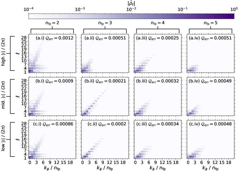
Figure 16: The FTSS is shown for 12 QH configurations from the QUASR database. The configurations are ordered by their number of field periods, which increases from the left (i) to the right (iv) column, and the absolute value of their rotational transform, which increases from the bottom (c) to the top (a) row. This ordering is further characterized by the annotations at the top and left side of the figure. The quasi-symmetry error of each configuration is recorded at the top right of each panel. These data demonstrate how the features of the linear shape distribution depends on the number of field periods, as described in the text.

In Fig. 16 the FTSS for 12 different QH equilibria are presented, with all configurations selected from the set of low $\mathcal{Q}_{\mathrm{err}}$ configurations in Fig. 15(a). The layout of Fig. 16 is analogous to that of Fig. 12. This means that $n_{\mathrm{fp}}$ increases from left to right along each row while $|\text{\sout{$\iota$}}|$ increases from the bottom to the top along each column. Each selected configuration has the lowest $\mathcal{Q}_{\mathrm{err}}$ among all the configurations in the respective row/column partition, and that quasi-symmetry error is shown in the top right of each panel. Here, the low $|\text{\sout{$\iota$}}|$ configurations in row (c) are constrained to $-1\leq\text{\sout{$\iota$}}>-7/6$, the middle $|\text{\sout{$\iota$}}|$ configurations in row (b) are constrained to $-7/6\leq\text{\sout{$\iota$}}>-8/6$, and the high $|\text{\sout{$\iota$}}|$ configurations in row (a) are constrained to $-8/6\leq\text{\sout{$\iota$}}>-3/2$.

In Fig. 16, considering the linear shape distribution along each row, one can observe two general trends. First, the slope of the distribution line tends to decrease with increasing $n_{\mathrm{fp}}$. Second, shape complexity tends to reduce as $n_{\mathrm{fp}}$ increases. This implies that the spatial resonance that results in a QH equilibria requires lower shape complexity and faster axial rotation as the number of field periods increases. Note, however, that since $k_{\phi}$ is normalized to an integer value of $n_{\mathrm{fp}}$, the increase in axial rotation with increasing $n_{\mathrm{fp}}$ is not due to the corresponding reduction in the toroidal domain of a given field period. This means the increase in axial rotation is an increase in the rotation per field period.

An additional trend can be observed along each column of Fig. 16. Namely, an increase in $|\text{\sout{$\iota$}}|$ is correlated with an increase in shape complexity. This is consistent with what was observed for the QA configurations in Fig. 12. However, unlike the QA data, an increase in $|\text{\sout{$\iota$}}|$ is not correlated with a decrease in the slope of the linear shape distribution in the QH configurations. Considering that the low $|\text{\sout{$\iota$}}|$ QH configurations all have a larger $|\text{\sout{$\iota$}}|$ than any of the high $|\text{\sout{$\iota$}}|$ QA configurations, this discrepancy implies a limit to the amount of rotational transform that can be driven by shape rotation. Above this limit, which is found at present to be $|\text{\sout{$\iota$}}|\approx 1$, a further increase in $|\text{\sout{$\iota$}}|$ may only result from increased shape complexity.

One notable exception to the trends described regarding both $n_{\mathrm{fp}}$ and $|\text{\sout{$\iota$}}|$ can be observed in panel (a.ii). This configuration exhibits both reduced shape complexity and a less dominant linear shape distribution relative to its neighboring configurations. However, this apparent outlier can also be observed to exhibit an anomalously large $\mathcal{Q}_{\mathrm{err}}$ relative to the other configurations within column (ii). Across all other columns, the largest percent difference in $\mathcal{Q}_{\mathrm{err}}$ between the largest and smallest value is observed in column (i), with a difference of 33%. In column (ii), between (a.ii) and (c.ii), this difference is 87%. Therefore, the configuration’s outlying character is likely attributed to its relatively poor quasi-symmetry.

It can also be observed that the three configurations in column (i) exhibit the largest quasi-symmetry errors in Fig. 16. From the corresponding FTSS, one finds the large errors are likely due to both higher-order shapes with little to no rotation about the magnetic axis (i.e., $\ell\leq 10$ and $k_{\phi}/n_{\mathrm{fp}}\approx 0$) and low-order shapes with large axial rotation (i.e., $\ell\leq 5$ and $k_{\phi}/n_{\mathrm{fp}}\approx 5$). Therefore, an optimization that aims to dampen these shaping modes may significantly improve the quasi-symmetry of the QH configurations with $n_{\mathrm{fp}}=2$.

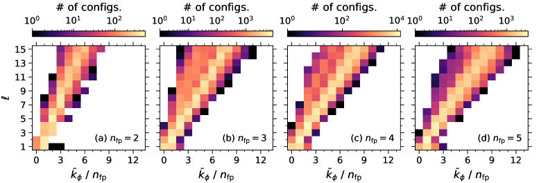
Figure 17: Four FTSS histograms are shown, comprised of QH configurations from the set of low $\mathcal{Q}_{\mathrm{err}}$ configurations in Fig. 15(a). Panels (a), (b), (c), and (d) are comprised of the $n_{\mathrm{fp}}=2$, $3$, $4$, and $5$ configurations, respectively. The histograms show the number of configurations that have the specified weighted average of $k_{\phi}$ for a given $\ell$. These data show that the QH resonance requires more rapid axial rotation when $n_{\mathrm{fp}}$ increases.

To highlight the dependence of the slope of the linear shape distribution on the number of field periods, Fig. 17 shows four additional FTSS histograms. All configurations in these four histograms are taken from the set of low $\mathcal{Q}_{\mathrm{err}}$ configurations of Fig. 15(a). From the left-most panel (a) to right-most panel (d) $n_{\mathrm{fp}}$ increases from $2$ to $5$, respectively. In panel (a), the histogram peak can be observed with a narrow $\bar{k}_{\phi}$ width and a steep $3/1$ distribution slope. Then, in panel (b), the histogram peak shifts to a $2/1$ distribution but with a broad $\bar{k}_{\phi}$ width. In panel (c), the distribution slope remains unchanged, but the $\bar{k}_{\phi}$ width is reduced. In panel (d), the $\bar{k}_{\phi}$ width is narrowed further and the $2/1$ slope remains. These observations clearly demonstrate a shift in $k_{\phi}$ to larger values with increasing $n_{\mathrm{fp}}$. Moreover, this implies that the QH resonance requires shaping modes to undergo more rapid axial rotation when the number of field periods is increased.

V Conclusion

A novel method for characterizing the shape of an ideal-MHD equilibrium has been presented. This method provides an equivalent shaping definition for both axisymmetric and non-axisymmetric equilibria, and, using a modal decomposition, invokes notions like elongation, triangularity, and squareness to any arbitrary order. Non-axisymmetric equilibria, however, were shown to have an additional degree of freedom, which is defined by the rate of rotation of the shaping modes about the magnetic axis.

Shaping spectra were analyzed for the precise QA and QH equilibria from Ref. Landreman et al. (2014) and compared against the initial configurations from which they were optimized. It was found that the shaping spectrum for both optimized configurations is dominated by an elongated shape that undergoes a $\pi$ rotation about the magnetic axis once per field period. Furthermore, over the course of their optimization, both the QA and QH configurations reveal a characteristic distribution of shaping modes about a line with slopes of $3/1$ and $2/1$, respectively. These slopes describe a proportionality between shape complexity and axial rotation, with smaller slopes indicating a faster increase in shape rotation for progressively higher-order shapes. These observations imply a spatial resonance between shape complexity and axial rotation that results in the precise quasi-symmetry of the two configurations.

In Sec. IV, the Fourier-transformed shaping spectra, and FTSS histograms, were presented for a subset of configurations from the QUASR database of non-axisymmetric equilibria. There, additional evidence was shown that the shaping distribution lines constitute an effective spatial description for quasi-symmetry. The slope of the line and the inclusion (or exclusion) of higher-order shaping modes is correlated with both the rotational transform and the number of field periods. Reducing the slope of the distribution line, so that higher-order modes undergo a faster axial rotation, one is able to increase the absolute value of the rotational transform while preserving the quasi-symmetry. Similarly, the inclusion of large-amplitude higher-order shaping modes (i.e., increased shape complexity) along a particular slope was shown to increase the rotational transform. However, with a high number of field periods, a comparable rotational transform can be achieved with lower amplitudes of the high-order modes (i.e., reduced shape complexity). In fact, increasing the number of field periods generally leads to reduced shape complexity, though eventually at the expense of quasi-symmetry.

The shaping analyses reported here are only an approximation. This is due to an inability to transform the magnetic axis to Boozer coordinates in VMEC. This error, however, was quantified, and the configurations analyzed were restricted to those for which the error is tolerably low. However, in future applications, it is desirable that the generalized shaping analysis be developed in equilibrium codes like DESC or GVEC, in which a transformation to Boozer coordinates along the magnetic axis is possible. It would also be informative to investigate the equilibrium shapes in a near-axis-expansion model, with the goal to provide an analytic foundation for the reported trends.

The goal in developing a robust and generalized framework for characterizing equilibrium shapes is, ultimately, to provide a means of systematically organizing the domain of toroidal equilibria and to support the optimization of those equilibria for various figures of merit. The methods reported here provide an important first step in that direction. Moreover, the most important contributions will likely come from using the macroscopic shaping analysis to investigate, inform, and predict changes in plasma stability and transport with respect to equilibrium shaping. Such an approach will enable the effective optimization of stellarator geometries.

Appendix A Error quantification in PEST coordinates

In VMEC, a flux surface geometry is represented by a Fourier series, defined in Appendix C, that depends on the poloidal $\theta_{v}$ and toroidal $\phi_{v}$ coordinates, where the toroidal VMEC angle is identical to the geometric angle $\phi_{v}=\varphi$. To transform VMEC flux-surface coordinates into Boozer coordinates, one may use the relations

$$\theta =\theta_{v}+\lambda(\psi,\,\theta_{v},\,\phi_{v})-\text{\sout{$\iota$}}p(\psi,\,\theta_{v},\,\phi_{v}),$$ (13)

$$\phi =\phi_{v}-p(\psi,\,\theta_{v},\,\phi_{v}).$$ (14)

Here $\lambda$ is a periodic stream function that transforms VMEC coordinates to straight-field-line PEST coordinates and $p$ is a periodic stream function that transforms PEST coordinates to Boozer coordinates boo .

The issue with using VMEC to compute the cross-sections arises from the fact that these stream functions $\lambda$ and $p$ are not defined for $\psi=0$. Therefore, one cannot transform $\phi_{v}$ to $\phi$ on the magnetic axis. This is not an issue for PEST coordinates, however, since $\phi_{v}$ is equivalent between VMEC and PEST. One may approximate Boozer coordinates with PEST coordinates, which is tantamount to assuming $\ell=0$ in Eqs. (13) and (14).

To justify this approximation, it is necessary to quantify the error it introduces. To accomplish this, first consider that the symmetry-aligned coordinates can be expressed as

$$\eta =\eta^{\prime}+\left(N-\text{\sout{$\iota$}}M\right)p,$$ (15)

$$\xi =\begin{cases}\xi^{\prime}-\left(\text{\sout{$\iota$}}/M\right)p,&\textrm{for \ QS}\\ \xi^{\prime}-\left(\text{\sout{$\iota$}}/M+1/N\right)p,&\mathrm{for\ QH}\end{cases}.$$ (16)

Here, $\eta^{\prime}$ and $\phi^{\prime}$ denote the corresponding angles as defined with PEST coordinates. Clearly, if $\ell=0$ then $\eta=\eta^{\prime}$ and $\xi=\xi^{\prime}$. Moreover, the differential relations $\partial\eta/\partial\eta=\partial\xi/\partial\xi=1$ and $\partial\eta/\partial\xi=\partial\xi/\partial\eta=0$ are satisfied everywhere. Therefore, to quantify the error associated with the assumption that $\eta=\eta^{\prime}$ and $\xi=\xi^{\prime}$, the relations

$$\frac{\partial\eta}{\partial\eta^{\prime}} =1+\left(N-\text{\sout{$\iota$}}M\right)\frac{\partial p}{\partial\eta^{\prime}},$$ (17)

$$\frac{\partial\eta}{\partial\xi^{\prime}} =\left(N-\text{\sout{$\iota$}}M\right)\frac{\partial p}{\partial\xi^{\prime}},$$ (18)

$$\frac{\partial\xi}{\partial\xi^{\prime}} =\begin{cases}1-\left(\text{\sout{$\iota$}}/M\right)\left(\partial p/\partial\xi^{\prime}\right),&\mathrm{for\ QA}\\ 1-\left(\text{\sout{$\iota$}}/M+1/N\right)\left(\partial p/\partial\xi^{\prime}\right),&\mathrm{for\ QH}\end{cases}$$ (19)

$$\frac{\partial\xi}{\partial\eta^{\prime}} =\begin{cases}-\left(\text{\sout{$\iota$}}/M\right)\left(\partial p/\partial\eta^{\prime}\right),&\mathrm{for\ QA}\\ -\left(\text{\sout{$\iota$}}/M+1/N\right)\left(\partial p/\partial\eta^{\prime}\right),&\mathrm{for\ QH}\end{cases}$$ (20)

are derived. Note that the differentials $\partial/\partial\eta^{\prime}$ and $\partial/\partial\xi^{\prime}$ are defined in terms of $\theta_{v}$ and $\phi_{v}$ in Appendix B, with the QA case defined in Eqs. (22)–(23) and the QH case defined in Eqs. (24)–(25). The local error $\mathcal{E}$ is then defined as

$$\mathcal{E}=\left[\left(\frac{\partial\eta}{\partial\eta^{\prime}}-1\right)^{2}+\left(\frac{\partial\eta}{\partial\xi^{\prime}}\right)^{2}+\left(\frac{\partial\xi}{\partial\xi^{\prime}}-1\right)^{2}+\left(\frac{\partial\xi}{\partial\eta^{\prime}}\right)^{2}\right]^{1/2}$$ (21)

To define a scalar-valued error, a flux-surface average is computed as $\langle\mathcal{E}\rangle=(1/A)\int\mathcal{E}dA$, where $dA=\sqrt{g}d\theta_{v}d\phi_{v}$ is a differential surface-area element with Jacobian $\sqrt{g}$, and $A=\int dA$ is the flux-surface area.

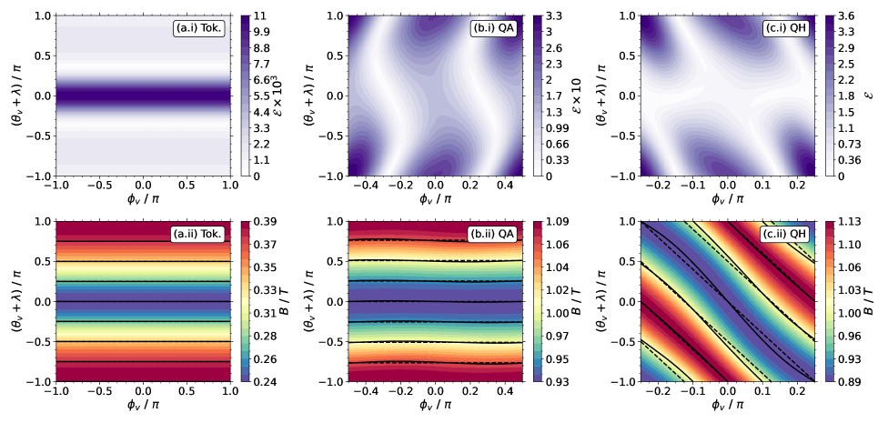
Figure 18: The top row shows the local error on the $\psi/\psi_{\mathrm{edge}}=0.5$ flux surface in PEST coordinates. The bottom row shows the magnetic field strength in the same coordinate system, with $\eta$ contours shown as solid black lines and $\eta^{\prime}$ shown as dashed black lines. The left, middle, and right columns show the tokamak with a circular cross-section, precise QA, and precise QH configurations, respectively. These plots demonstrate the effectiveness of the local error calculation at capturing the misalignment between symmetry and PEST coordinates.

In Fig. 18, the local error is shown for the tokamak with a circular cross-section, the precise QA, and precise QH configurations in panels (a.i)–(c.i), respectively. For comparison, panels (a.ii)–(c.ii) show $B$ as a function of the poloidal and toroidal angles in PEST coordinates. In each magnetic-field-strength plot, contours of $\eta$ are shown as solid black lines and contours of $\eta^{\prime}$ are shown as dashed black lines.

From the figure, it can be observed that the largest local error occurs on the outboard side ($\theta_{v}+\lambda=0$) of the tokamak and the inboard side ($\theta_{v}+\lambda=\pm\pi$) for both stellarator configurations. Moreover, along the outboard side of the stellarators, the maximal error is localized to the points where the $\eta^{\prime}$ curves cross the $\eta$ curves, which is to be expected since these are the locations of maximal deviation in coordinate alignment. Evaluating the flux-surface average of Eq. (21) in all three configurations results in $\langle\mathcal{E}\rangle=2.94\times 10^{-3}$, $0.121$, and $1.08$ for the tokamak, QA, and QH configurations, respectively. Based on these results, a maximum allowable $\langle\mathcal{E}\rangle$ for any configuration whose shaping analysis is presented in this paper is set to $1.25$.

Appendix B Computing PEST Coordinate Differentials

The chain rule is used to define the the $\eta^{\prime}$ and $\xi^{\prime}$ differentials with respect to the VMEC flux-surface coordinates, with $\psi$ being held fixed, so that

$$\frac{\partial}{\partial\eta^{\prime}} =\frac{\partial\theta_{v}}{\partial\eta^{\prime}}\frac{\partial}{\partial\theta_{v}}+\frac{\partial\phi_{v}}{\partial\eta^{\prime}}\frac{\partial}{\partial\phi_{v}},$$

$$\frac{\partial}{\partial\xi^{\prime}} =\frac{\partial\theta_{v}}{\partial\xi^{\prime}}\frac{\partial}{\partial\theta_{v}}+\frac{\partial\phi_{v}}{\partial\xi^{\prime}}\frac{\partial}{\partial\phi_{v}}.$$

To compute these differentials, one must derive an expression for the differentials of the VMEC coordinates with respect to $\eta^{\prime}$ and $\xi^{\prime}$. To that end, consider that

$$\eta^{\prime} =M\left(\theta_{v}+\lambda\right)-N\phi_{v},$$

$$\xi^{\prime} =\begin{cases}\phi_{v}/M,&\textrm{for \ QA}\\ \left(\theta_{v}+\lambda\right)/M-\phi_{v}/N,&\textrm{for \ QS}\end{cases}.$$

Taking the $\eta^{\prime}$ and $\xi^{\prime}$ differentials and solving the resulting system of equations, one finds that, for the QA case,

$$\frac{\partial\theta_{v}}{\partial\eta^{\prime}} =\frac{1}{M}\left(1+\frac{\partial\lambda}{\partial\theta_{v}}\right)^{-1}$$

$$\frac{\partial\phi_{v}}{\partial\eta^{\prime}} =0$$

$$\frac{\partial\theta_{v}}{\partial\xi^{\prime}} =-M\left(1+\frac{\partial\lambda}{\partial\theta_{v}}\right)^{-1}\frac{\partial\lambda}{\partial\phi_{v}}$$

$$\frac{\partial\phi_{v}}{\partial\xi^{\prime}} =M.$$

Therefore, the symmetry-aligned PEST differentials are defined

$$\frac{\partial}{\partial\eta^{\prime}} =\frac{1}{M}\left(1+\frac{\partial\lambda}{\partial\theta_{v}}\right)^{-1}\frac{\partial}{\partial\theta_{v}},$$ (22)

$$\frac{\partial}{\partial\xi^{\prime}} =-M\left[\left(1+\frac{\partial\lambda}{\partial\theta_{v}}\right)^{-1}\frac{\partial}{\partial\theta_{v}}-\frac{\partial}{\partial\phi_{v}}\right].$$ (23)

Following the same procedure for the QH case, one finds

$$\frac{\partial\theta_{v}}{\partial\eta^{\prime}} =\frac{N}{N^{2}-M^{2}}\left(1+\frac{\partial\lambda}{\partial\theta_{v}}\right)^{-1}\left(\frac{M}{N}+\frac{\partial\lambda}{\partial\phi_{v}}\right)$$

$$\frac{\partial\phi_{v}}{\partial\eta^{\prime}} =\frac{-N}{N^{2}-M^{2}}$$

$$\frac{\partial\theta_{v}}{\partial\xi^{\prime}} =\frac{NM^{2}}{N^{2}+M^{2}}\left(1+\frac{\partial\lambda}{\partial\theta_{v}}\right)^{-1}\left(\frac{N}{M}-\frac{\partial\lambda}{\partial\phi_{v}}\right)$$

$$\frac{\partial\phi_{v}}{\partial\xi^{\prime}} =\frac{NM^{2}}{N^{2}+M^{2}}.$$

The resulting differentials are then

$$\frac{\partial}{\partial\eta^{\prime}} =\frac{N}{N^{2}-M^{2}}\left[\left(1+\frac{\partial\lambda}{\partial\theta_{v}}\right)^{-1}\left(\frac{M}{N}+\frac{\partial\lambda}{\partial\phi_{v}}\right)\frac{\partial}{\partial\theta_{v}}-\frac{\partial}{\partial\phi_{v}}\right],$$ (24)

$$\frac{\partial}{\partial\xi^{\prime}} =\frac{NM^{2}}{N^{2}+M^{2}}\left[\left(1+\frac{\partial\lambda}{\partial\theta_{v}}\right)^{-1}\left(\frac{N}{M}-\frac{\partial\lambda}{\partial\phi_{v}}\right)\frac{\partial}{\partial\theta_{v}}+\frac{\partial}{\partial\phi_{v}}\right].$$ (25)

Appendix C Computing the Covariant Basis Vectors

In VMEC, the cylindrical coordinates $R$ and $Z$ and the stream function $\lambda$ are defined as

$$R =\sum_{m=0}^{\mathcal{M}}\sum_{n=-\mathcal{N}}^{\mathcal{N}}R_{mn}(\psi)\cos(m\theta_{v}-nn_{\mathrm{fp}}\phi_{v}),$$

$$Z =\sum_{m=0}^{\mathcal{M}}\sum_{n=-\mathcal{N}}^{\mathcal{N}}Z_{mn}(\psi)\sin(m\theta-nn_{\mathrm{fp}}\phi),$$

$$\lambda =\sum_{m=0}^{\mathcal{M}}\sum_{n=-\mathcal{N}}^{\mathcal{N}}L_{mn}(\psi)\sin(m\theta-nn_{\mathrm{fp}}\zeta).$$

Here $R_{mn}$, $Z_{mn}$, and $L_{mn}$ are the radially-dependent Fourier amplitudes and $\mathcal{M}$ and $\mathcal{N}$ are the number of cosidered poloidal and toroidal mode numbers, respectively.

The covariant basis vectors in any three-dimensional coordinate system are defined as $\mathbf{e}_{i}=\partial\mathbf{r}/\partial\alpha_{i}$ for the $i^{\mathrm{th}}$ coordinate, where $\mathbf{r}=R\hat{\mathbf{e}}_{R}+Z\hat{\mathbf{e}}_{Z}$ and $\hat{\mathbf{e}}_{R}$, $\hat{\mathbf{e}}_{\varphi}$, and $\hat{\mathbf{e}}_{Z}$ are the normalized cylindrical basis vectors. The covariant VMEC basis vectors are then defined as

$$\mathbf{e}_{\psi} =\frac{\partial R}{\partial\psi}\hat{\mathbf{e}}_{\mathrm{R}}+\frac{\partial Z}{\partial\psi}\hat{\mathbf{e}}_{\mathrm{Z}},$$

$$\mathbf{e}_{\theta} =\frac{\partial R}{\partial\theta_{v}}\hat{\mathbf{e}}_{\mathrm{R}}+\frac{\partial Z}{\partial\theta_{v}}\hat{\mathbf{e}}_{\mathrm{Z}},$$

$$\mathbf{e}_{\phi} =\frac{\partial R}{\partial\phi_{v}}\hat{\mathbf{e}}_{\mathrm{R}}+R\hat{\mathbf{e}}_{\varphi}+\frac{\partial Z}{\partial\phi_{v}}\hat{\mathbf{e}}_{\mathrm{Z}}.$$

Using Eqs. (22)–(23), the covariant basis vectors in PEST coordinates are, for the QA case,

$$\mathbf{e}_{\eta} =\frac{1}{M}\left(1+\frac{\partial\lambda}{\partial\theta_{v}}\right)^{-1}\mathbf{e}_{\phi},$$ (26)

$$\mathbf{e}_{\xi} =-M\left[\left(1+\frac{\partial\lambda}{\partial\theta_{v}}\right)^{-1}\mathbf{e}_{\theta}-\mathbf{e}_{\phi}\right].$$ (27)

Similarly, using Eqs. (24)–(25), the covariant basis vectors for the QH case are

$$\mathbf{e}_{\eta} =\frac{N}{N^{2}-M^{2}}\left[\left(1+\frac{\partial\lambda}{\partial\theta_{v}}\right)^{-1}\left(\frac{M}{N}+\frac{\partial\lambda}{\partial\phi_{v}}\right)\mathbf{e}_{\theta}-\mathbf{e}_{\phi}\right],$$ (28)

$$\mathbf{e}_{\xi} =\frac{NM^{2}}{N^{2}+M^{2}}\left[\left(1+\frac{\partial\lambda}{\partial\theta_{v}}\right)^{-1}\left(\frac{N}{M}-\frac{\partial\lambda}{\partial\phi_{v}}\right)\mathbf{e}_{\theta}+\mathbf{e}_{\phi}\right].$$ (29)

References

- Scarabosio et al. (2007) A. Scarabosio, A. Pochelon, and Y. Martin, Plasma Phys. Control. Fusion 49, 1041 (2007).
- Brunetti et al. (2020) D. Brunetti, C. J. Ham, J. P. Graves, C. Wahlberg, and W. A. Cooper, Plasma Phys. Control. Fusion 62, 115005 (2020).
- Rodríguez (2023) E. Rodríguez, J. Plasma Phys. 89, 905890211 (2023).
- Bindel et al. (2023) D. Bindel, M. Landreman, and M. Padidar, Plasma Phys. Control. Fusion 65, 065012 (2023).
- Beidler et al. (2021) C. D. Beidler et al., Nature 596, 221 (2021).
- Canik et al. (2007a) J. M. Canik, D. T. Anderson, F. S. B. Anderson, C. Clark, K. M. Likin, J. N. Talmadge, and K. Zhai, Phys. Plasmas 14, 056107 (2007a).
- Canik et al. (2007b) J. M. Canik, D. T. Anderson, F. S. B. Anderson, K. M. Likin, J. N. Talmadge, and K. Zhai, Phys. Rev. Lett. 98, 085002 (2007b).
- Angelino et al. (2009) P. Angelino, X. Garbet, L. Villard, A. Bottino, S. Jolliet, P. Ghendrih, V. Grandgirard, B. F. McMillan, Y. Sarazin, G. Dif-Pradalier, and T. M. Tran, Phys. Rev. Lett. 102, 195002 (2009).
- Mynick et al. (2010) H. E. Mynick, N. Pomphrey, and P. Xanthopoulos, Phys. Rev. Lett. 105, 095004 (2010).
- Xanthopoulos et al. (2014) P. Xanthopoulos, H. E. Mynick, P. Helander, Y. Turkin, G. G. Plunk, F. Jenko, T. Görler, D. Told, T. Bird, and J. H. E. Proll, Phys. Rev. Lett. 113, 155001 (2014).
- Proll et al. (2015) J. H. E. Proll, H. E. Mynick, P. Xanthopoulos, S. A. Lazerson, and B. J. Faber, Plasma Phys. Control. Fusion 58, 014006 (2015).
- Hegna et al. (2018) C. C. Hegna, P. W. Terry, and B. J. Faber, Phys. Plasmas 25, 022511 (2018).
- Terry et al. (2018) P. W. Terry, B. J. Faber, C. C. Hegna, V. V. Mirnov, M. J. Pueschel, and G. G. Whelan, Phys. Plasmas 25, 012308 (2018).
- Fontana et al. (2017) M. Fontana, L. Porte, S. Coda, O. Sauter, and T. T. Team, Nucl. Fusion 58, 024002 (2017).
- Huang et al. (2018) Z. Huang, S. Coda, and the TCV team, Plasma Phys. Contr. Fusion 61, 014021 (2018).
- Laribi et al. (2021) E. Laribi, E. Serre, P. Tamain, and H. Yang, Nucl. Mater. Energy 27, 101012 (2021).
- Nakata and Matsuoka (2022) M. Nakata and S. Matsuoka, Plasma Fusion Res. 17, 1203077 (2022).
- Mackenbach et al. (2022) R. J. J. Mackenbach, J. H. E. Proll, and P. Helander, Phys. Rev. Lett. 128, 175001 (2022).
- Roberg-Clark et al. (2022) G. T. Roberg-Clark, G. G. Plunk, and P. Xanthopoulos, Phys. Rev. Res. 4, L032028 (2022).
- Merlo et al. (2023) G. Merlo, M. Dicorato, B. Allen, T. Dannert, K. Germaschewski, and F. Jenko, Phys. Plasmas 30, 102302 (2023).
- Gerard et al. (2023) M. J. Gerard, B. Geiger, M. J. Pueschel, A. Bader, C. C. Hegna, B. J. Faber, P. W. Terry, S. T. A. Kumar, and J. C. Schmitt, Nucl. Fusion 63, 056004 (2023).
- Gerard et al. (2024) M. Gerard, M. Pueschel, B. Geiger, R. Mackenbach, J. Duff, B. Faber, C. Hegna, and P. Terry, Phys. Plasmas 31, 052501 (2024).
- Goodman et al. (2024) A. G. Goodman, P. Xanthopoulos, G. G. Plunk, H. Smith, C. Nührenberg, C. D. Beidler, S. A. Henneberg, G. Roberg-Clark, M. Drevlak, and P. Helander, PRX Energy 3, 023010 (2024).
- Miller et al. (1998) R. L. Miller, M. S. Chu, J. M. Greene, Y. R. Lin-Liu, and R. E. Waltz, Phys. Plasmas 5, 973 (1998).
- Weisen et al. (1997) H. Weisen, J.-M. Moret, S. Franke, I. Furno, Y. Martin, M. Anton, R. Behn, M. Dutch, B. Duval, F. Hofmann, B. Joye, C. Nieswand, Z. Pietrzyk, and W. V. Toledo, Nucl. Fusion 37, 1741 (1997).
- Waltz and Miller (1999) R. E. Waltz and R. L. Miller, Phys. Plasmas 6, 4265 (1999).
- Reimerdes et al. (2000) H. Reimerdes, A. Pochelon, O. Sauter, T. P. Goodman, M. A. Henderson, and A. Martynov, Plasma Phys. Control. Fusion 42, 629 (2000).
- Ball and Parra (2017) J. Ball and F. I. Parra, Plasma Phys. Control. Fusion 59, 024007 (2017).
- Marinoni et al. (2021) A. Marinoni, O. Sauter, and S. Coda, Rev. Mod. Plasma Phys. 5, 6 (2021).
- Beeke et al. (2021) O. Beeke, M. Barnes, M. Romanelli, M. Nakata, and M. Yoshida, Nucl. Fusion 61, 066020 (2021).
- Mercier (1964) C. Mercier, 4, 213 (1964).
- Solov’ev and Shafranov (1970) L. S. Solov’ev and V. D. Shafranov, Reviews of Plasma Physics, 5, 1 (1970).
- Lortz and Nührenberg (1976) D. Lortz and J. Nührenberg, Z. Naturforsch. A 31, 1277 (1976).
- Garren and Boozer (1991) D. A. Garren and A. H. Boozer, Phys. Fluids B 3, 2805 (1991).
- Hegna (2000) C. C. Hegna, Phys. Plasmas 7, 3921 (2000).
- Hegna (2015) C. C. Hegna, Phys. Plasmas 22, 072510 (2015).
- Helander (2014) P. Helander, Rep. Prog. Phys. 77, 087001 (2014).
- Landreman and Paul (2022) M. Landreman and E. J. Paul, Phys. Rev. Lett. 128, 035001 (2022).
- Giuliani et al. (2022a) A. Giuliani, F. Wechsung, A. Cerfon, G. Stadler, and M. Landreman, J. Comput. Phys. 459, 111147 (2022a).
- Giuliani et al. (2022b) A. Giuliani, F. Wechsung, G. Stadler, A. Cerfon, and M. Landreman, J. Plasma Phys. 88, 905880401 (2022b).
- Giuliani et al. (2023) A. Giuliani, F. Wechsung, A. Cerfon, M. Landreman, and G. Stadler, Phys. Plasmas 30, 042511 (2023).
- Antonsen et al. (2019) T. Antonsen, E. J. Paul, and M. Landreman, J. Plasma Phys. 85, 905850207 (2019).
- Paul et al. (2020) E. J. Paul, T. Antonsen, M. Landreman, and W. A. Cooper, J. Plasma Phys. 86, 905860103 (2020).
- Paul et al. (2021) E. J. Paul, M. Landreman, and T. Antonsen, J. Plasma Phys. 87, 905870214 (2021).
- Boozer (1980) A. H. Boozer, Phys. Fluids 23, 904 (1980).
- D’haeseleer et al. (1991) W. D. D’haeseleer, W. N. G. Hitchon, J. D. Callen, and J. L. Shohet, Flux Coordinates and Magnetic Field Structure (Springer, Berlin, Heidelberg, 1991).
- Hirshman and Whitson (1983) S. Hirshman and J. Whitson, Phys. Fluids 26, 3553 (1983).
- (48) See https://princetonuniversity.github.io/STELLOPT/ for details.
- Giuliani (2024) A. Giuliani, 10.5281/zenodo.13717741 (2024).
- Dudt and Kolemen (2020) D. W. Dudt and E. Kolemen, Phys. Plasmas 27, 102513 (2020).
- Hindenlang et al. (2025) F. Hindenlang, R. Babin, O. Maj, T. Ribeiro, R. Koeberl, D. Muir, G. G. Plunk, and E. Sonnendrücker, Gvec: A flexible 3d mhd equilibrium solver (2025).
- Landreman et al. (2014) M. Landreman, H. M. Smith, A. Mollén, and P. Helander, Phys. Plasmas 21, 042503 (2014).