Decentralized Optimization over Time-Varying Row-Stochastic Digraphs

Abstract

Decentralized optimization over directed graphs is essential for applications such as robotic swarms, sensor networks, and distributed learning. In many practical scenarios, the underlying network is a Time-Varying Broadcast Network (TVBN), where only row-stochastic mixing matrices can be constructed due to inaccessible out-degree information. Achieving exact convergence over TVBNs has remained a long-standing open question, as the limiting distribution of time-varying row-stochastic mixing matrices depends on unpredictable future graph realizations, rendering standard bias-correction techniques infeasible.

This paper resolves this open question by developing the first algorithm that achieves exact convergence using only time-varying row-stochastic matrices. We propose PULM (Pull-with-Memory), a gossip protocol that attains average consensus with exponential convergence by alternating between row-stochastic mixing and local adjustment. Building on PULM, we develop PULM-DGD, which converges to a stationary solution at $\mathcal{O}(\ln(T)/T)$ for smooth nonconvex objectives. Our results significantly extend decentralized optimization to highly dynamic communication environments.

1 Introduction

This paper investigates decentralized optimization over a network of $n$ nodes:

$$\min_{x\in\mathbb{R}^{d}}\quad f(x):=\frac{1}{n}\sum_{i=1}^{n}f_{i}(x).$$ (1)

Each objective function $f_{i}$ is accessible only by node $i$ and is assumed to be smooth and potentially nonconvex. The local losses $f_{i}$ generally differ from each other, which poses challenges to both the design and analysis of distributed algorithms.

Decentralized optimization eliminates the need for a central server, thereby enhancing flexibility and enabling broad applicability in edge-to-edge communication scenarios. Consequently, the design of distributed optimization algorithms is strongly influenced by the underlying communication network among nodes, which is typically modeled as a graph or characterized by a mixing matrix. This study focuses on decentralized optimization over directed graphs, or digraphs. Directed communication provides an appropriate model for numerous real-world scenarios, including robotic swarms with asymmetric linkages [saber2003agreement, shorinwa2024distributed], sensor networks supporting unidirectional message transmission [sang2010link, kar2008distributed], and distributed deep learning systems in which bandwidth asymmetry constrains communication [zhang2020network, liang2024communication].

1.1 Time-Varying Broadcast Network.

The need for distributed optimization over directed graphs arises from complex communication constraints in real-world scenarios. Depending on the nature of these constraints, the underlying digraph may exhibit various challenging properties, including (1) not being weight-balanced, (2) having a time-varying topology, and (3) nodes lacking knowledge of their own out-degrees. In the most demanding communication settings, all three properties must be addressed simultaneously. We refer to a network exhibiting all these characteristics as a Time-Varying Broadcast Network (TVBN).

In many practical applications, the communication setting can only be accurately modeled as a TVBN. The following three examples illustrate such scenarios.

Example 1 (Random Radio Broadcast).

In radio communications, transmitted information is received by any node within broadcast range, and the sender has no knowledge of which nodes have received the message. The network topology varies over time as nodes enter or exit the broadcast range.

Example 2 (Byzantine Attack).

A Byzantine attack occurs when a subset of agents in the system behaves maliciously or transmits corrupted information to other nodes. Nodes receiving such malicious information may attempt to ignore or discard these unreliable signals, resulting in a TVBN.

Example 3 (Packet Loss and Network Failure).

When packet loss or network failure occurs, receivers obtain incomplete or corrupted messages, creating uncertainty regarding the status of message delivery. Such scenarios can be modeled as a TVBN.

While decentralized optimization over time-varying digraphs has been extensively studied, all existing results, to our knowledge, require nodes to be aware of their out-degrees. Building upon the push-sum protocol, seminal works [nedic2014distributed, nedic2016stochastic, nedic2017achieving] investigate decentralized algorithms over time-varying column-stochastic networks. To ensure column-stochastic mixing matrices, each node must know its out-degree, which is not feasible in highly dynamic communication environments. Even if a node correctly determines its out-degree and scales the weights accordingly for its neighbors, a network failure occurring after transmission (but before reception) may prevent some neighbors from receiving the message. In this case, the effective out-degree changes unexpectedly, and column-stochasticity can no longer be guaranteed; see Figure 1 for an illustration. Another important line of work [saadatniaki2020decentralized, nedic2023ab, nguyen2023accelerated] studies push-pull or AB algorithms over time-varying digraphs. Since these methods alternately rely on row-stochastic and column-stochastic matrices, they also require out-degree knowledge. In fact, only algorithms relying purely on row-stochastic mixing matrices are feasible in TVBNs, since each node only needs to know its in-degree, which is naturally immune to highly dynamic communication environments; see Figure 1 for an illustration.

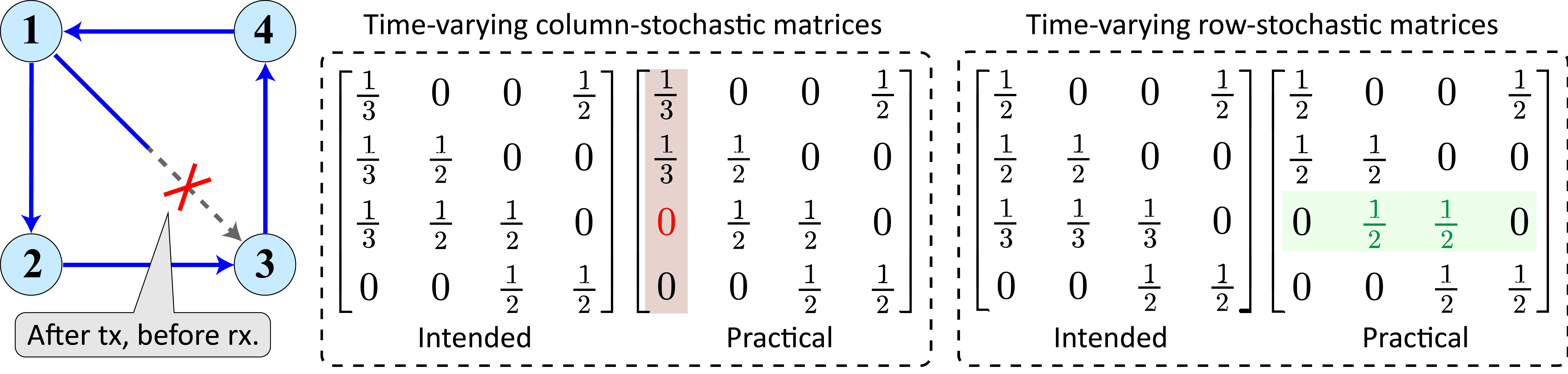
Figure 1: Left: A time-varying network with $n=4$ nodes experiencing partial network failure; “tx” and “rx” denote “transmission” and “reception,” respectively. Middle and right: The corresponding column- and row-stochastic mixing matrices. The network failure results in an incorrect column-stochastic matrix due to sudden changes in out-degree information. However, a correct row-stochastic matrix can still be constructed since it relies only on in-degree information, which remains accessible.

1.2 Open Questions and Challenges

Decentralized optimization over time-varying column-stochastic digraphs is now well understood, with foundational methods [nedic2014distributed, akbari2015distributed, nedic2016stochastic] developed over a decade ago and subsequently extended by [nedic2017achieving, saadatniaki2020decentralized]. However, developing algorithms that exactly solve problem (1) over purely time-varying row-stochastic digraphs (i.e., TVBNs) remains a long-standing open question.

Since the out-degree is inaccessible in TVBNs, even developing decentralized algorithms to achieve average consensus is challenging. Assume each node $i\in[n]$ in the network initializes a vector $x_{i}$. Traditional gossip algorithms [boyd2006randomized, aysal2009broadcast] can only achieve consensus among nodes in TVBNs, but not average consensus $n^{-1}\sum_{i=1}^{n}x_{i}$. The approach most related to our setting is that of [mai2016distributed], which proposes a pre-correction strategy for static row-stochastic mixing matrices. This strategy exploits the following property: for a nonnegative row-stochastic matrix $A$ with strong connectivity, there exists a unique Perron vector $\pi_{A}$ (i.e., $\pi_{A}>0$, $\pi_{A}^{\top}A=\pi_{A}^{\top}$, $\mathds{1}_{n}^{\top}\pi_{A}=1$) satisfying

$$A^{k}\to\mathds{1}_{n}\pi_{A}^{\top},\quad k\to\infty.$$

Using this property, [mai2016distributed] initializes $z^{(0)}_{i}=(n[\pi_{A}]_{i})^{-1}x_{i}$ at each node and iteratively propagate $z_{i}$ over the network (which is equivalent to left-multiplying by $A$):

$$z^{(k)}=A^{k}\mathrm{diag}(n\pi_{A})^{-1}x^{(0)}\to\mathds{1}_{n}\pi_{A}^{\top}\mathrm{diag}(n\pi_{A})^{-1}x^{(0)}=n^{-1}\mathds{1}_{n}\mathds{1}_{n}^{\top}x^{(0)},\quad k\to\infty,$$

where we let $z^{(k)}:=[(z^{(k)}_{1})^{\top};(z^{(k)}_{2})^{\top};\cdots;(z^{(k)}_{n})^{\top}]$ and $x^{(0)}:=[x_{1}^{\top};x_{2}^{\top};\cdots;x_{n}^{\top}]$.

However, this approach does not extend to time-varying row-stochastic matrices $A^{(k)}$. For the product $\Phi(k+B,k)=A^{(k+B-1)}\cdots A^{(k)}$, the limiting matrix is

$$\Phi(k+B,k)\to\mathds{1}_{n}\pi_{k}^{\top},\quad B\to\infty,$$

where $\pi_{k}$ is a limiting vector depends on the entire unpredictable future sequence $\{A^{(t)}\}_{t\geq k}$. To see it, the above relation implies $\pi_{k}^{\top}=\pi_{k+1}^{\top}A^{(k)}=\pi_{k+2}^{\top}A^{(k+1)}A^{(k)}=\pi_{k+3}^{\top}A^{(k+2)}A^{(k+1)}A^{(k)}=\cdots$, revealing that $\pi_{k}$ depends on future sequence $\{A^{(t)}\}_{t\geq k}$. Consequently, $\pi_{k}$ cannot be estimated from past observations $\{A^{(t)}\}_{t\leq k}$ alone, and no pre-correction at initialization can uniformly eliminate the consensus bias across all admissible time-varying sequences. Since average consensus is the essential building block for decentralized optimization, its failure renders the overarching optimization problem exceptionally challenging.

1.3 Related Work

In connected networks, the topology is characterized by a mixing matrix. For undirected networks, constructing symmetric and doubly stochastic mixing matrices is straightforward. Early decentralized algorithms for such settings include decentralized gradient descent (DGD) [nedic2009distributed], diffusion [chen2012diffusion], and dual averaging [duchi2011dual]. These methods, however, exhibit bias under data heterogeneity [yuan2016convergence]. To address this limitation, advanced algorithms have been developed based on explicit bias-correction [shi2015extra, yuan2018exact, li2019decentralized] and gradient tracking [xu2015augmented, di2016next, nedic2017achieving, qu2017harnessing]. Extending these algorithms to time-varying undirected networks [nedic2017achieving, maros2018panda] is natural, as time-varying doubly stochastic mixing matrices readily preserve essential average consensus properties.

For directed networks, constructing doubly stochastic matrices is generally infeasible. When the out-degree of each node is accessible, column-stochastic mixing matrices can be constructed [nedic2014distributed, tsianos2012push]. Decentralized algorithms using such column-stochastic matrices are well studied. They leverage the push-sum technique [kempe2003gossip, tsianos2012push] to correct the bias in column-stochastic communications and achieve global averaging of variables or gradients. While the subgradient-push algorithm [nedic2014distributed, tsianos2012push] guarantees convergence to optimality, its sublinear rate persists even under strong convexity. Subsequent work—including EXTRA-push [zeng2017extrapush], D-EXTRA [xi2017dextra], ADD-OPT [xi2017add], and Push-DIGing [nedic2017achieving]—has achieved faster convergence by explicitly mitigating heterogeneity. Recent work [liang2023towards] has established lower bounds and optimal algorithms for decentralized optimization over column-stochastic digraphs. Since the push-sum technique naturally accommodates time-varying column-stochastic digraphs, all the aforementioned algorithms readily extend to such settings.

When only in-degree information is available, one can construct row-stochastic mixing matrices. Diffusion [chen2012diffusion, sayed2014adaptive] was among the earliest decentralized algorithms using row-stochastic mixing matrices, but converges only to a Pareto-optimal solution rather than the global optimum. Just as push-sum underpins column-stochastic algorithms, the pull-diag gossip protocol [mai2016distributed] serves as an effective technique to correct the bias caused by row-stochastic communications. Reference [xi2018linear] first adapted distributed gradient descent to this setting. Subsequently, gradient tracking techniques were extended to the row-stochastic scenario by [li2019row, FROST-Xinran, liangachieving], while momentum-based variants were developed in [ghaderyan2023fast, lu2020nesterov]. However, all of these algorithms are designed exclusively for static row-stochastic digraphs. To the best of our knowledge, no existing algorithm can achieve exact convergence to the solution of problem (1) using purely row-stochastic mixing matrices due to the challenges discussed in Section 1.2.

In digraphs where both in-degree and out-degree information are available, the Push-Pull/AB methods [pu2020push, xin2018linear, you2025stochastic, liang2025linear] can solve problem (1) by alternately using column-stochastic and row-stochastic mixing matrices [nedic2025ab, akgun2024projected]. These algorithms typically achieve faster convergence than methods relying solely on column- or row-stochastic matrices and can handle both static and time-varying scenarios. However, they require knowledge of the in-degree at each node, which is unavailable in TVBNs.

1.4 Main Results

This paper develops the first algorithm to achieve exact convergence for problem (1) using only time-varying row-stochastic mixing matrices, thereby making decentralized optimization feasible over TVBNs and significantly enhancing its robustness to highly dynamic environments. Our results are:

• Effective average consensus protocol. We propose PULL-with-Memory (PULM), a decentralized gossip protocol that achieves average consensus over time-varying row-stochastic broadcast digraphs. By alternating between a standard row-stochastic gossip step and a local adjustment step, we theoretically prove that PULM converges to average consensus exponentially fast.

• The first exactly converging algorithm. Built upon PULM, we develop a decentralized gradient descent approach over TVBNs, termed PULM-DGD. For nonconvex and smooth optimization problems, we establish that PULM-DGD converges to a stationary solution at a rate of ${\mathcal{O}}(\frac{\ln(K)}{K})$. To the best of our knowledge, PULM-DGD is the first algorithm that achieves exact convergence using only time-varying row-stochastic mixing matrices.

Organization. The remainder of this paper is organized as follows. Notation and assumptions are provided in Section 2. In Section 3, we examine the mixing dynamics in TVBNs and derive our PULM approach for achieving distributed average consensus. Performing decentralized optimization through PULM is discussed in Section 4, where we provide the main convergence theorems. We conduct numerical experiments to verify the effectiveness of PULM and PULM-DGD in Section 5 and conclude in Section 6.

2 Notations and Assumptions

In this section, we declare necessary notations and assumptions.

Notations. Let $\mathds{1}_{n}$ denote the vector of all-ones of $n$ dimensions and $I_{n}\in\mathbb{R}^{n\times n}$ the identity matrix. We denote $E_{n}:=\frac{1}{n}\mathds{1}_{n}\mathds{1}_{n}^{\top}$. We use $[n]$ to denote the set $\{1,2,\ldots,n\}$. For a given vector $v$, $\mathrm{Diag}(v)$ signifies the diagonal matrix whose diagonal elements are comprised of $v$. We define $n\times d$ matrices

$${\mathbf{x}}^{(k)} \hskip-1.42262pt:=\hskip-1.42262pt[({x}_{1}^{(k)})^{\top}\hskip-1.42262pt;({x}_{2}^{(k)})^{\top}\hskip-1.42262pt;\cdots;({x}_{n}^{(k)})^{\top}\hskip-1.42262pt]$$

$$\hskip-1.42262pt{\mathbf{g}}^{(k)} \hskip-1.42262pt:=\hskip-1.42262pt[\nabla F_{1}({x}_{1}^{(k)};\hskip-1.42262pt\xi_{1}^{(k)})^{\top}\hskip-1.42262pt;\hskip-1.42262pt\cdots\hskip-1.42262pt;\hskip-1.42262pt\nabla F_{n}({x}_{n}^{(k)};\xi_{n}^{(k)})^{\top}\hskip-1.42262pt]$$

$$\nabla f({\mathbf{x}}^{(k)}) \hskip-1.42262pt:=\hskip-1.42262pt[\nabla f_{1}({x}^{(k)}_{1})^{\top};\cdots;\nabla f_{n}({x}^{(k)}_{n})^{\top}]$$

by stacking all local variables vertically. The upright bold symbols (e.g. ${\mathbf{x}},{\mathbf{g}}$) always denote network-level quantities. For vectors or matrices, we use the symbol $\leq$ for element-wise comparison. We use $\|\cdot\|$ for $\ell_{2}$ vector norm and $\|\cdot\|_{F}$ for matrix Frobenius norm. We use $\|\cdot\|_{2}$ for induced $\ell_{2}$ matrix norm, which means $\|A\|_{2}:=\max_{\|v\|=1}\|Av\|$. Unless otherwise specified, product signs for matrices always indicate consecutive left multiplication in order, i.e., $\prod_{k=1}^{K}A^{(i)}:=A^{(K)}A^{(K-1)}\cdots A^{(2)}A^{(1)}$. When a directed graph ${\mathcal{G}}$ is strongly connected, it means there exists a directed path from $i$ to $j$ for any nodes $i,j$ in ${\mathcal{G}}$.

Gossip communication. When node $i$ collects information $x_{j}\in\mathbb{R}^{d},j\in N_{i}^{\rm{in}}$ from its in-neighbors, it can mix these vectors using scalars $a_{ij}$, producing $x_{i}^{\text{new}}=\sum_{j\in N_{i}^{\rm{in}}}a_{ij}x_{j}$. This process is called gossip communication. Using the stacked notation ${\mathbf{x}}=[x_{1}^{\top};x_{2}^{\top};\ldots;x_{n}^{\top}]$ and $A=[a_{ij}]_{n\times n}$, the update can be written as ${\mathbf{x}}^{\text{new}}\leftarrow A{\mathbf{x}}$, where $A$ is called the mixing matrix. When out-degrees are accessible, $A$ can be constructed as either column-stochastic or row-stochastic. When out-degrees are inaccessible, $A$ can only be row-stochastic.

Assumptions. The following assumptions are used throughout this paper.

Assumption 1 ($\tilde{B}$-Strongly Connected Graph Sequence).

The time-varying directed graph sequence $\{\mathcal{G}^{(k)}=(\mathcal{V},\mathcal{E}^{(k)})\}_{k\geq 0}$ satisfies the following: there exists an integer $\tilde{B}>0$ such that for any $k\geq 0$, the $\tilde{B}$-step accumulated graph

$$\mathcal{G}_{k}^{\tilde{B}}:=\left(\mathcal{V},\bigcup_{l=k}^{k+\tilde{B}-1}\mathcal{E}^{(l)}\right)$$

is strongly connected. Additionally, each graph $\mathcal{G}^{(k)}$ contains a self-loop at every node.

Assumption 2 (Rapidly Changing Broadcast Network).

For each $k\geq 0$ and $i\in[n]$, node $i$ does not know its out-degree $d_{i}^{{\rm{out}},(k)}$ in graph ${\mathcal{G}}^{(k)}$. Additionally, for each $k\geq 0$, the mixing matrix generated from ${\mathcal{G}}^{(k)}$ can only be used once.

The single-use constraint on mixing matrices in Assumption 2 reflects the rapidly changing topology: by the time communication using $A^{(k)}$ completes, the network has already transitioned to ${\mathcal{G}}^{(k+1)}$, making $A^{(k)}$ incompatible with the current network structure. This is typical in highly dynamic environments such as mobile ad-hoc networks or drone swarms.

Definition 1 (Compatible Mixing Matrices).

A mixing matrix $A=[a_{ij}]_{n\times n}$ is compatible with graph ${\mathcal{G}}$ if

$$a_{ij}>0\text{ if }(j\to i)\in{\mathcal{E}},\text{ and }a_{ij}=0\text{ otherwise}.$$

Any compatible $A$ for ${\mathcal{G}}$ satisfying Assumption 2 is row-stochastic, i.e., $A\mathds{1}_{n}=\mathds{1}_{n}$.

Assumption 3 (Lower Bounded Entries).

Suppose that for each $k\geq 0$, we have a mixing matrix $A^{(k)}$ that is compatible with ${\mathcal{G}}^{(k)}$. There exists a scalar $\tau>0$ such that all nonzero entries of $A^{(k)}$ satisfy $a^{(k)}_{ij}\geq\tau$ for all $k\geq 0$.

Assumption 3 is naturally satisfied by setting $A^{(k)}_{ij}=1/d_{i}^{\mathrm{in},(k)}$ and $\tau=1/n$.

Proposition 1.

Suppose Assumptions 1 and 3 hold. Then there exist an integer $0<B<n\tilde{B}$ and a scalar $\eta\in[\tau^{B},1)$ such that

$$\Phi(k+B,k):=\prod_{l=0}^{B-1}A^{(k+l)}\geq\eta,\quad\forall k\geq 0.$$

Proposition 1 establishes that, for any starting time $k$, the $B$-step product of mixing matrices $\Phi(k+B,k)$ is entrywise lower bounded by a constant $\eta>0$. This property is central to the convergence analysis: it implies uniform mixing over every $B$-step window, ensuring that each node’s information influences every other node with weight at least $\eta$, independent of $k$. We next introduce our final assumption.

Assumption 4 (Smoothness).

There exist constants $L,\Delta\geq 0$ such that for all $i\in[n]$ and all ${x},{y}\in\mathbb{R}^{d}$,

$$\left\|\nabla f_{i}({x})-\nabla f_{i}({y})\right\|\leq L\|{x}-{y}\|,\quad\mbox{and}\quad f_{i}({x}^{(0)})-\inf_{{x}\in\mathbb{R}^{d}}f_{i}({x})\leq\Delta.$$

3 Achieving Average Consensus over TVBN

In this section, we analyze how information are mixed and propagated across TVBNs using row-stochastic mixing matrices only. To formalize this process, let each node $i$ initialize a vector $z_{i}^{(0)}=x_{i}$. The $k$-th communication round is governed by the row-stochastic mixing matrix $A^{(k)}$. At the beginning of the $k$-th round, we assume each node $i$ stores a vector $z_{i}^{(k)}$, which can be expressed as a linear combination of all initial vectors:

$$z_{i}^{(k)}=\sum_{j=1}^{n}w_{ij}^{(k)}x_{j},$$ (2)

where $w^{(k)}_{ij}$ are some weights at iteration $k$. Without loss of generality, we assume the initial vectors $\{x_{i}\}_{i=1}^{n}$ are linearly independent, which ensures that the coefficients $\{w_{ij}^{(k)}\}$ are uniquely determined. We term process (2) the mixing dynamics.

3.1 Mixing Dynamics over TVBNs

By collecting coefficients $w_{ij}^{(k)}$ in (2), we define the distribution matrix $W^{(k)}\coloneqq[w_{ij}^{(k)}]_{i,j=1}^{n}\in\mathbb{R}^{n\times n},$ which maps the initial vectors $\{x_{j}\}_{j=1}^{n}$ to the node states at round $k$. In particular, letting $z^{(k)}\coloneqq\big[z_{1}^{(k)},\ldots,z_{n}^{(k)}\big]^{\top}$ and $x\coloneqq\big[x_{1},\ldots,x_{n}\big]^{\top}$, the mixing dynamics (2) can be written compactly as $z^{(k)}=W^{(k)}x$. At initialization, each node stores its own vector $z_{i}^{(0)}:=x_{i}$, hence $W^{(0)}=I_{n}$. Moreover, average consensus is achieved if $W^{(k)}\to\tfrac{1}{n}\mathds{1}_{n}\mathds{1}_{n}^{\top}\text{as }k\to\infty.$ Using the mixing dynamics in (2), the gossip update $z_{i}^{(k+1)}=\sum_{j=1}^{n}a_{ij}^{(k)}z_{j}^{(k)}$ is equivalent to performing the following matrix update

$$W^{(k+1)}=A^{(k)}W^{(k)},$$ (3)

where $A^{(k)}=[a_{ij}^{(k)}]_{n\times n}$ is row-stochastic. However, the simple gossip update (3) cannot drive $W^{(k)}$ to $n^{-1}\mathds{1}_{n}\mathds{1}_{n}^{\top}$. Instead, it converges to a biased average:

Proposition 2 (Limiting Property).

For $\{{\mathcal{G}}^{(k)},A^{(k)}\}_{k\geq 0}$ satisfying Assumptions 1–3, define $\Phi(k+B,k)=\prod_{i=0}^{B-1}A^{(k+i)}$. It follows that $\lim_{k\to\infty}\Phi(k+B,k)=\mathds{1}_{n}\pi_{k}^{\top},\forall$, where $\pi_{k}\in\mathbb{R}^{n}$ is determined by the sequence $\{A^{(t)}\}_{t\geq k}$. Moreover, the convergence occurs at an exponential rate.

Proof.

See Appendix B.3. ∎

While Proposition 2 guarantees asymptotic consensus, the limit is a $\pi_{k}$-weighted average rather than the average consensus $n^{-1}\sum_{i=1}^{n}x_{i}$. Moreover, since $\pi_{k}$ is determined entirely by the future sequence $\{A^{(t)}\}_{t\geq k}$, for any past sequence $\{A^{(t)}\}_{t<k}$, one can construct infinitely many future sequences (all satisfying the connectivity and weight assumptions) that yield any desired stochastic vector $\pi_{k}$. Thus, past observations provide no information about $\pi_{k}$, which poses a fundamental challenge for pre-correction as discussed in Section 1.2. We illustrate this in the example below.

Example 1.

Consider a two-node network with row-stochastic matrices

$$A_{1}=\begin{pmatrix}0.9&0.1\\ 0.5&0.5\end{pmatrix},\quad A_{2}=\begin{pmatrix}0.5&0.5\\ 0.1&0.9\end{pmatrix}.$$

Suppose $A^{(k)}=A_{1}$ for all $k<t$. If $A^{(k)}=A_{1}$ for $k\geq t$, then $\pi_{k}=(5/6,1/6)^{\top}$; whereas if $A^{(k)}=A_{2}$ for $k\geq t$, then $\pi_{k}=(1/6,5/6)^{\top}$. Since the past sequences are identical, no estimator relying on past $\{A^{(t)}\}_{t<k}$ can predict $\pi_{k}$.

3.2 Shifting the Limits toward Average Consensus

Our method leverages a simple observation: since the limiting distribution $\pi_{k}$ depends on the entire sequence of mixing matrices, judicious modifications of the intermediate $W^{(k)}$ can steer $\pi_{k}$ toward any desired value. Specifically, before left-multiplying by $A^{(k)}$, we introduce an adjustment step designed to shift the limiting vector closer to the uniform distribution. Through repeated adjustments, the process is progressively driven toward the desired average $n^{-1}\mathds{1}_{n}$. This two-stage process can be represented as:

$$\cdots\longrightarrow W^{(k)}\overset{A^{(k)}}{\longrightarrow}W^{(k+\frac{1}{2})}\overset{\text{adjust}}{\longrightarrow}W^{(k+1)}\overset{A^{(k+1)}}{\longrightarrow}W^{(k+1+\frac{1}{2})}\overset{\text{adjust}}{\longrightarrow}W^{(k+2)}{\longrightarrow}\cdots,$$

where $\overset{A^{(k)}}{\longrightarrow}$ denotes the gossip step and $\overset{\text{adjust}}{\longrightarrow}$ denotes the adjustment step. Crucially, this adjustment must be communication-free and rely on locally available information.

Algorithm 1 Matrix-level procedure for driving $W^{(k)}$ to $n^{-1}\mathds{1}_{n}\mathds{1}_{n}^{\top}$

1:Initialize $W^{(0)}=I_{n}$.

2:for $k=0,1,2,\ldots,K-1$ do

3:  $W^{(k+\frac{1}{2})}=A^{(k)}W^{(k)}$;

4:  Replace the diagonal entries of $W^{(k+\frac{1}{2})}$ by $\frac{1}{n}$, and name it $W^{(k+1)}$;

5:end for

6:Output: $W^{(K)}$

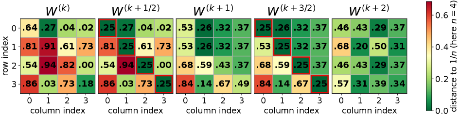
Figure 2: Diffusion of the $1/n$ diagonal anchor under the adjust–gossip update. The adjust step anchors each diagonal entry $w^{(k+\frac{1}{2})}_{jj}$ at $1/n$; the gossip step then diffuses this value down column $j$, pulling off-diagonal entries toward $1/n$. Cell colors indicate distance to $1/n$ (greener means closer), showing how the anchored mass spreads from the diagonal throughout each column, driving $W^{(k)}$ toward average consensus.

Algorithm 1 summarizes our proposed procedure. The intuition behind why it drives $W^{(k)}$ toward $n^{-1}\mathds{1}_{n}\mathds{1}_{n}^{\top}$ is straightforward: Each iteration alternates between an adjust step, which resets diagonal entries to $1/n$, and a gossip step, which computes $W^{(k+1)}=A^{(k)}W^{(k+\frac{1}{2})}$ via convex combinations of rows. Although gossip averages across rows, its effect manifests column-wise: entries within each column are repeatedly mixed, progressively converging to the same value. Since column $j$ always contains the anchored value $W^{(k+\frac{1}{2})}_{jj}=1/n$, this mixing pulls off-diagonal entries toward $1/n$—effectively diffusing the anchor throughout the column (see Figure 2). Over successive iterations, all entries converge to $1/n$, yielding average consensus.

Figure 3: Convergence of $W^{(k)}$. The definition of “W Error” and details of different topologies can be found in Appendix E.7.

We illustrate the performance of Algorithm 1 with a simple numerical simulation, demonstrating that the procedure converges exponentially fast to average consensus over various time-varying networks using row-stochastic matrices (see Figure 3). A node-wise implementation of Algorithm 1 is provided in Algorithm 2. We name this algorithm PULM (Pull with Memory) because gossiping with a row-stochastic matrix is commonly referred to as a “pull” operation, and our method additionally requires each node to store and update its distribution vector $w_{i}^{(k)}$, which serves as a “memory” of the mixing process. The following theorem establishes that PULM achieves monotonic and exponentially fast convergence.

Algorithm 2 Pull with Memory (PULM)

1:Input: Vector $x_{i}\in\mathbb{R}^{d}$ at each node $i\in[n]$ to be averaged

2:for each node $i\in[n]$ in parallel do

3:  Initialize $z_{i}^{(0)}=x_{i}$ and $w_{i}^{(0)}=\bm{e}_{i}$, where $\bm{e}_{i}$ is the $i$-th column of $I_{n}$

4:  for $k=0,1,2,\ldots,K-1$ do

5:   Gossip: $z_{i}^{(k+\frac{1}{2})}=\sum_{j=1}^{n}a_{ij}^{(k)}z_{j}^{(k)}$ and $w_{i}^{(k+\frac{1}{2})}=\sum_{j=1}^{n}a_{ij}^{(k)}w_{j}^{(k)}$

6:   Adjust: $d_{i}^{(k)}=[w_{i}^{(k+\frac{1}{2})}]_{i}-\frac{1}{n}$

7:   Update: $z_{i}^{(k+1)}=z_{i}^{(k+\frac{1}{2})}-d_{i}^{(k)}\cdot x_{i}$ and $w_{i}^{(k+1)}=w_{i}^{(k+\frac{1}{2}}-d_{i}^{(k)}\cdot\bm{e}_{i}$

8:  end for

9:end for

10:Output: $z_{i}^{(K)}$ at each node $i\in[n]$

Theorem 1.

For $\{{\mathcal{G}}^{(k)}\}_{k\geq 0}$ satisfying Assumptions 1 and 2, and $\{A^{(k)}\}_{k\geq 0}$ satisfying Assumption 3, the following statements hold:

1. In Algorithm 1, the sequence $\{\max_{i,j}|[W^{(k)}]_{ij}-n^{-1}|\}_{k\geq 0}$ is non-increasing.

2. In both Algorithms 1 and 2,

   $$\|W^{(K)}-n^{-1}\mathds{1}_{n}\mathds{1}_{n}^{\top}\|_{F}\leq\frac{n}{1-\eta}(1-\eta)^{K/B}.$$

3. In Algorithm 2,

   $$\|{\mathbf{z}}^{(K)}-n^{-1}\mathds{1}_{n}\mathds{1}_{n}^{\top}{\mathbf{x}}^{(0)}\|_{F}\leq\frac{n}{1-\eta}(1-\eta)^{K/B}\|{\mathbf{x}}^{(0)}\|_{F}.$$

Here, the constants $B>0$ and $\eta\in(0,1)$ are defined in Proposition 1.

Proof.

See Appendix C.1. ∎

Remark 1 (Column-stochastic vs. row-stochastic matrices).

Average consensus is comparatively easy to achieve over time-varying networks when column-stochastic weights are available. In this case, the required correction admits a simple forward recursion that can be maintained incrementally as the network evolves. In contrast, with row-stochastic weights, the analogous correction requires backward-in-time propagation through the matrix sequence, which cannot be computed online using only past information. See Appendix A for more details.

4 Decentralized Optimization over TVBN

In this section, we present Algorithm 3, the first decentralized optimization algorithm that achieves exact convergence over TVBNs. The algorithm employs a double-loop structure. At the beginning of each outer iteration $k$, every node $i$ computes and stores its local gradient $g_{i}^{(k)}=\nabla f_{i}(x_{i}^{(k)})$. The inner loop then executes two parallel consensus processes, as illustrated in (4).

$$x_{i}^{(k)}\xmapsto{\text{Gossip}}\hat{x}_{i}^{(k)}\rightarrow x_{i}^{(k+1)}$$

$$\downarrow\hskip 42.67912pt{\uparrow}\hskip 56.9055ptk\text{-th iteration of PULM-DGD}$$ (4)

$$g_{i}^{(k)}\xmapsto{\text{PULM}}\hskip 2.84526pt\hat{g}_{i}^{(k)}$$

• Gradient averaging. The PULM protocol (Algorithm 2) is applied to the local gradients $\{g_{i}^{(k)}\}$ to compute an accurate average $\hat{g}^{(k)}_{i}\approx\frac{1}{n}\sum_{j=1}^{n}g_{j}^{(k)}$.

• Parameter mixing. A standard gossip protocol is applied to the parameters $\{x_{i}^{(k)}\}$ to reach a biased consensus $\hat{x}_{i}^{(k)}\approx\pi^{\top}{\mathbf{x}}^{(k)}$, where $\pi$ is a weight vector determined by the TVBN topology.

The outer loop update is $x_{i}^{(k+1)}=\hat{x}_{i}^{(k)}-\alpha\hat{g}^{(k)}_{i}$, where $\alpha>0$ is the step size. This structure closely resembles centralized gradient descent, with the key difference being that each node uses consensus-based approximations of the global gradient and parameter average.

Algorithm 3 PULM-based Decentralized Gradient Descent (PULM-DGD)

1:Input: Step size $\gamma>0$, inner iterations $\{R_{k}\}_{k\geq 0}$

2:for each node $i\in[n]$ in parallel do

3:  Initialize all variables to the same arbitrary value $x_{i}^{(0)}=x^{(0)}$

4:  for $k=0,1,2,\ldots,K-1$ do

5:   Compute local gradient: $g_{i}^{(k)}=\nabla f_{i}(x_{i}^{(k)})$

6:   Initialize $z_{i}^{(k,0)}=x_{i}^{(k)}-\gamma g_{i}^{(k)}$ and $w_{i}^{(k,0)}=\bm{e}_{i}$

7:   for $r=0,1,2,\ldots,R_{k}-1$ do $\triangleright$ PULM inner loop

8:     Gossip: $z_{i}^{(k,r+\frac{1}{2})}=\sum_{j=1}^{n}a_{ij}^{(k,r)}z_{j}^{(k,r)}$, $w_{i}^{(k,r+\frac{1}{2})}=\sum_{j=1}^{n}a_{ij}^{(k,r)}w_{j}^{(k,r)}$

9:     Adjust: $d_{i}^{(k,r)}=[w_{i}^{(k,r+\frac{1}{2})}]_{i}-\frac{1}{n}$

10:     Update: $z_{i}^{(k,r+1)}=z_{i}^{(k,r+\frac{1}{2})}-d_{i}^{(k,r)}g_{i}^{(k)}$, $w_{i}^{(k,r+1)}=w_{i}^{(k,r+\frac{1}{2})}-d_{i}^{(k,r)}\bm{e}_{i}$

11:   end for

12:   $x_{i}^{(k+1)}=z_{i}^{(k,R_{k})}$

13:  end for

14:end for

15:Output: $x_{i}^{(K)}$ at each node $i\in[n]$

In practice, communicating the parameters $x_{i}^{(k)}$ and gradients $g_{i}^{(k)}$ through separate channels would be inefficient. Algorithm 3 optimizes this process by performing a local gradient step first (line 4), allowing nodes to communicate only a single combined state vector $z_{i}^{(k,r)}$ in each inner iteration (lines 6–9). This significantly reduces the total communication cost compared to naive implementations that would require separate consensus processes for parameters and gradients.

Now we state the main convergence results. We use the notation $W^{(k,r)}=[w_{ij}^{(k,r)}]_{n\times n}$ in the following theorem.

Theorem 2.

Suppose Assumption 1, 2 and 3 hold. To simplify the notations, in Algorithm 3 we further assume that there exists $C_{W}>0$ and $0\leq\beta_{W}<1$ such that $\|W^{(k,r)}-n^{-1}\mathds{1}_{n}\mathds{1}_{n}^{\top}\|_{2}\leq C_{W}\beta_{W}^{r}$ for all $k$ and $r$. When $\gamma\leq\frac{1}{24nC_{W}^{2}L}$ and $R_{k}\geq\max\{\frac{\ln(C_{W})}{1-\beta_{W}},\frac{\ln(k)}{1-\beta_{W}}\}$, we have

$$\frac{1}{K}\sum_{k=0}^{K-1}\|\nabla f(\bar{x}^{(k)})\|^{2}\leq\frac{18\Delta}{\gamma K},\quad\text{ where }\bar{x}^{(k)}=\frac{1}{n}\sum_{i=1}^{n}x_{i}^{(k)}.$$

By choosing $\gamma=\frac{1}{n24C_{W}^{2}L}$ and $R_{k}=\max\{\frac{\ln(C_{W})}{1-\beta_{W}},\frac{\ln(k)}{1-\beta_{W}}\}$ for all $k\geq 0$, we have

$$\frac{1}{K}\sum_{k=0}^{K-1}\|\nabla f(\bar{x}^{(k)})\|^{2}\leq\frac{432nC_{W}^{2}L\Delta}{K},$$ (5)

and the total number of communication rounds equals to

$$\sum_{k=0}^{K-1}R_{k}\leq\max\{\sum_{k=1}^{K-1}\frac{\ln(k)}{1-\beta_{W}},\sum_{k=1}^{K-1}\frac{\ln(C_{W})}{1-\beta_{W}}\}=\frac{\max\{K\ln(K),K\ln(C_{W})\}}{1-\beta_{W}}.$$

In Theorem 2, when we define the total number of communication rounds $T=\sum_{k=0}^{K-1}R_{k}$, we obtain $K={\mathcal{O}}(T/\ln(T))$. Plugging this into (5) results in an overall convergence rate of ${\mathcal{O}}(\frac{\ln(T)}{T})$.

5 Experiments

To verify the effectiveness of Algorithms 2 and 3, we conducted extensive experiments on a series of problems over various time-varying network topologies. The problem types we considered are summarized as: (i) consensus problem; (ii) logistic regression with non-convex regularization and (iii) neural network training for MNIST and CIFAR-10 classification. In this section, we only demonstrate several representative experimental results. Further supplementary experiments, the details of problem setting and network topology selection strategies can be found in Appendix E.

5.1 Comparison with Push-Family Algorithms

Push-DIGing [nedic2017achieving] and its consensus counterpart, Push-Sum [kempe2003gossip] are among the few methods that explicitly address time-varying directed networks. Nevertheless, push-based schemes typically require knowledge of the out-degrees to construct properly normalized (column-stochastic) mixing weights. Under packet loss, the effective out-degree becomes random and time-varying: although a node attempts to transmit to its out-neighbors, only a subset of messages is successfully received. Since the nominal out-degree does not reflect these successful deliveries, the resulting weights may violate the algorithm’s normalization conditions. As a result, Push-DIGing can become unstable and may fail to converge in packet-loss networks. Meanwhile, PULM-Family remains robust, see Figure 4.

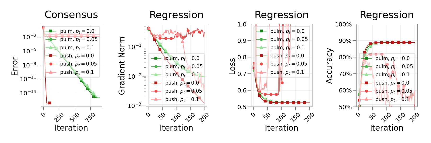
Figure 4: Performance comparison of push-family and PULM-family algorithms under packet loss on time-varying directed networks. In consensus, push denotes push-sum and pulm denotes PULM; in regression, push denotes push-DIGing and pulm denotes PULM-DGD. The packet-loss probability at time $t$ is $p_{t}$. See Appendix E.1 for full experimental settings.

The first sub-figure in Fig. 4 reports average-consensus performance with $N=20$ nodes and randomly generated data of dimension $d=1024$; the communication graph is resampled each interval with sparsity $s=0.2$. The remaining sub-figures report regression on synthetic data: $10$ nodes each hold $1000$ samples with $30$ features, the heterogeneity parameter is $\sigma_{h}=0.1$, and the stepsize is $\gamma=0.1$. Communication is based on a strongly connected graph of sparsity $0.3$, with link disconnections occurring with probability $p_{d}=0.4$, and the inner communication rounds are fixed as $R_{k}\equiv 10$. Across all cases, the push-family methods (push-sum and push-DIGing) are highly sensitive to packet loss—even $p_{t}=0.05$ can prevent convergence—whereas PULM and PULM-DGD remain robust, consistent with the fact that they do not rely on out-degree information for normalization.

5.2 Effect of Different Inner Communication Rounds $R_{k}$

The inner communication rounds $R_{k}$ control how much mixing (i.e., consensus refinement) is performed per outer iteration and therefore directly determine the communication cost. Theorem 2 provides a sufficient choice, requiring $R_{k}$ to grow on the order of $\ln(k)$ to guarantee the stated convergence bound. In practice, however, we often observe that constant values of $R_{k}$ already yield nearly identical optimization performance, suggesting that the theoretical schedule is conservative. We next quantify this effect empirically.

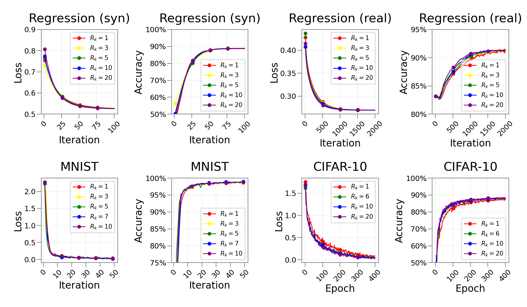
Figure 5: Effect of the inner communication rounds $R_{k}$ on the performance of Algorithm 3. Top row: logistic regression on synthetic data (loss and accuracy) and on real data (loss and accuracy) for $R_{k}\in\{1,3,5,10,20\}$. Bottom row: MNIST training (loss and accuracy) for $R_{k}\in\{1,3,5,7,10\}$, and CIFAR-10 training (loss and accuracy) for $R_{k}\in\{1,6,10,20\}$. Larger $R_{k}$ increases communication per outer iteration but yields only marginal changes in convergence behavior. See Appendix E.5 for experimental details.

Figure 5 indicates that changing the inner communication rounds $R_{k}$ mainly affects communication cost rather than the final performance. Across logistic regression, MNIST, and CIFAR-10, the loss/accuracy curves for different $R_{k}$ are close and often nearly overlap, suggesting that Algorithm 3 is not particularly sensitive to this hyper-parameter. Larger $R_{k}$ can slightly improve the early-stage progress by enhancing mixing, but the benefit quickly saturates; hence, a small constant $R_{k}$ is typically sufficient in practice.

6 Conclusion

In this paper, we studied average consensus over time-varying broadcast networks (TVBNs). We showed that the limiting Perron (influence) vector induced by the mixing process can be future-dependent; consequently, the common strategy of estimating the limiting Perron vector and applying an inverse correction is not applicable in TVBNs. To address this difficulty, we proposed PULM, a row-stochastic, broadcast-compatible protocol motivated by the mixing-dynamics analysis, and proved that it achieves average consensus at an exponential rate. We further integrated PULM with distributed gradient descent to obtain PULM-DGD: model parameters are propagated via standard broadcast communication, while incremental gradients are mixed using the PULM protocol, which improves communication efficiency. Under nonconvex objectives (under the assumptions specified in our analysis), PULM-DGD attains a near-linear convergence rate. Numerical experiments corroborate the effectiveness of the proposed algorithms.

Appendix A Achieving Average Consensus Using Column Stochastic Matrices

In this section, we briefly explain why average consensus is comparatively easy to obtain over time-varying networks when column-stochastic weights are available. Suppose there exists a sequence of column-stochastic matrices $\{B^{(k)}\}_{k\geq 1}$ compatible with the graph sequence $\{{\mathcal{G}}^{(k)}\}_{k\geq 1}$ and satisfying Assumption 1. Then it can be shown that

$$\lim_{k\to\infty}\mathrm{Diag}\!\big(B^{(k)}B^{(k-1)}\cdots B^{(1)}\mathds{1}_{n}\big)^{-1}\,B^{(k)}B^{(k-1)}\cdots B^{(1)}\;=\;n^{-1}\mathds{1}_{n}\mathds{1}_{n}^{\top}.$$ (6)

The reason is that the required normalizer admits a simple online recursion. Indeed, letting $v_{k}:=B^{(k)}B^{(k-1)}\cdots B^{(1)}\mathds{1}_{n}$ with $v_{0}=\mathds{1}_{n}$, we obtain $v_{k+1}=B^{(k+1)}v_{k}.$ Hence $\mathrm{Diag}(v_{k})^{-1}$ can be maintained incrementally as the network evolves, which makes the normalization in (6) readily implementable.

In contrast, when only row-stochastic matrices $\{A^{(k)}\}_{k\geq 1}$ are available, the analogous normalization takes the dual forms

$$\lim_{k\to\infty}A^{(k)}A^{(k-1)}\cdots A^{(1)}\,\mathrm{Diag}\,\!\big(\mathds{1}_{n}^{\top}A^{(k)}A^{(k-1)}\cdots A^{(1)}\big)^{-1}\;=\;n^{-1}\mathds{1}_{n}\mathds{1}_{n}^{\top}.$$ (7)

Here the normalizer $\mathds{1}_{n}^{\top}A^{(k)}A^{(k-1)}\cdots A^{(1)}$ corresponds (after transposition) to the vector $u_{k}:=A^{(1)\top}A^{(2)\top}\cdots A^{(k)\top}\mathds{1}_{n}.$ However, computing $u_{k}$ requires a backward-in-time propagation through $A^{(k)},A^{(k-1)},\ldots,A^{(1)}$, which is not implementable in a time-varying network.

Appendix B Proofs of Lemmas

B.1 Proof of Proposition 1

Proof.

Given starting time $k$, starting node $s\in\mathcal{V}$ and ending node $e\in\mathcal{V}$, our goal is to find a finite state transition trajectory from $s$ to $e$. Since the directed graphs always contain self loop, it is trivial to find a trajectory when $s=e$. And when $s\neq e$, we define the sets of nodes which have already been searched as $\mathcal{V}_{\ominus}$, and initiate it as $\mathcal{V}_{\ominus}=\{s\}$, to which we will add more nodes later. Meanwhile, we introduce two notations: (1) $v_{1}\rightarrow v_{2}$ means there exists a path from $v_{1}$ to $v_{2}$ for a given graph $\mathcal{G}$ ($\mathcal{G}$ may be an accumulated graph as demonstrated in Assumption 1.); (2) $v_{1}\xrightarrow{t}v_{2}$ means that $v_{1}$ sends information to $v_{2}$ exactly during the time interval $t$.

The searching process can be broken down into the following steps.

Step 1. Use Assumption 1, during $\tilde{B}$ time intervals, we can find at least one path from $s$ to $e$, from which we pick out a shortest path $s\to v_{1}\to\dots\to e$. If $v_{1}=e$, the searching process can be finished. Otherwise we add $v_{1}$ into $\mathcal{V}_{\ominus}$, and there exist at least one time point $t_{1}\in[k,k+\tilde{B}-1]$ such that $(s,v_{1})\in\mathcal{E}^{(t_{1})}$, we construct the transition trajectory as

$$s\xrightarrow{k}s\xrightarrow{k+1}\cdots s\xrightarrow{t_{1}-1}s\xrightarrow{t_{1}}v_{1}$$

Step 2. Changing starting node as $v_{1}$ and time point as $t+1$, using Assumption 1 again, during $\tilde{B}$ time intervals, we can find at least one path from $v_{1}$ to $e$, from which we pick out a shortest path $v_{1}\to v_{2}\to\dots\to e$. The searching process ends if $v_{2}=e$. Otherwise, if $v_{2}\neq e$ and $v_{2}\notin\mathcal{V}_{\ominus}$, we can further add $v_{2}$ into $\mathcal{V}_{\ominus}$ and repeat the above process. However, if $v_{2}\in\mathcal{V}_{\ominus}$, we should find the first new node $v_{*}\notin\mathcal{V}_{\ominus}$ from the path $v_{1}\to v_{2}\to\dots\to v_{+}\to v_{*}\to\cdots\to e$ and a time point $t_{*}\in[t_{1}+1,t_{1}+\tilde{B}]$ such that $(v_{+},v_{*})\in\mathcal{E}^{(t_{*})}$, where $v_{+}$ is the last point which still stays in $\mathcal{V}_{\ominus}$. In this case, we retrace our trajectory back to the node $v_{+}$ and keep it until the time point $t_{*}$, i.e.,

$$s\xrightarrow{k}s\xrightarrow{k+1}\cdots\xrightarrow{t_{+}}v_{+}\xrightarrow{t_{+}+1}\cdots v_{+}\xrightarrow{t_{*}}v_{*},$$

where $t_{+}$ is the first time point $v_{+}$ was searched. Consequently, we can use $v_{*}$ instead of $v_{2}$ as the new search point and repeat the above process.

…

These steps will be repeated no more than $n$ times. We can find a state transition trajectory starting at time point $k$ from $s$ to $e$ whose length $B$ is no longer than $n\tilde{B}$. According to Assumption 3, the transition probability $\eta$ from $s$ to $e$ during $B$ time intervals can be lower bounded by $\tau^{n\tilde{B}}$. All of the constants are not related to time points $k$ and nodes indices, so the existence of $B$ and $\eta$ is proved. ∎

B.2 Linear Convergence Lemma

Lemma 1.

For a sequence of row-stochastic matrices $\tilde{A}^{(1)},\tilde{A}^{(2)},\dots\in\mathbb{R}^{n\times n}$, assuming $\tilde{A}^{(t)}_{i,j}\geq\eta>0,~\forall i,j\in[n],~\forall t=1,2,\dots$, we have

1. The limit $\tilde{A}^{\infty}:=\prod_{t=1}^{+\infty}\tilde{A}^{(t)}$ exists. And $\tilde{A}^{\infty}$ is a row-stochastic matrix with identical rows, i.e.,

   $$\tilde{A}^{\infty}=\mathds{1}_{n}\pi^{\top},$$

   where $\pi$ is an asymptotical steady distribution.

2. The maximum deviation converges with geometric rate, i.e.

   $$\max\bigg|\prod_{t=1}^{T}\tilde{A}^{(t)}-\tilde{A}^{\infty}\bigg|\leq\frac{1+\eta}{\eta}(1-\eta)^{T}$$

Proof.

The process of proof here is adapted from that in [nedic2009distributed, nedic_convergence_2010]. However, our lemma can be more easily used under milder Assumptions 1, 2 and 3 which [nedic2009distributed, nedic_convergence_2010] did not introduce.

1. Consider an arbitrary vector $\bm{x}^{(0)}\in\mathbb{R}^{n}$, we are going to prove that the limit of $\bm{x}^{(t)}:=\tilde{A}^{(t)}\cdots\tilde{A}^{(1)}\bm{x}^{(0)}$ exists. Note that $\bm{x}^{(t)}$ can be decomposed into a consensus part and a surplus part, i.e.,

$$\bm{x}^{(t)}=p^{(t)}\mathds{1}_{n}+\bm{z}^{(t)},\quad\bm{z}^{(t)}\geq 0.$$ (8)

where $p^{(t)}$ is a scalar and $\bm{z}^{(t)}$ is a vector. Our goal is to construct a Cauchy sequence $\{p^{(t)}\}_{t=0}^{\infty}$ and $\{\bm{z}^{(t)}\}_{t=0}^{\infty}\to\bm{0}$. We first choose

$$p^{(0)}=\min_{1\leq i\leq n}\{\bm{x}^{(0)}_{i}\},\quad\bm{z}^{(0)}=\bm{x}^{(0)}-\min_{1\leq i\leq n}\{\bm{x}^{(0)}_{i}\}\mathds{1}_{n}.$$

Using the decomposition, the recursion of $\bm{x}^{(t)}$ can be expanded as

$$\bm{x}^{(t+1)}=\tilde{A}^{(t+1)}\bm{x}^{(t)}=\tilde{A}^{(t+1)}(p^{(t)}\mathds{1}_{n}+\bm{z}^{(t)})=p^{(t)}\mathds{1}_{n}+\tilde{A}^{(t+1)}\bm{z}^{(t)}.$$

We define the index $i^{*}$ as

$$i^{*}:=\mathop{\arg\min}_{1\leq i\leq n}\tilde{A}^{(t+1)}_{i,\cdot}\bm{z}^{(t)},$$

which means $\min_{1\leq i\leq n}\{\tilde{A}^{(t+1)}_{i,\cdot}\bm{z}^{(t)}\}=\tilde{A}^{(t+1)}_{i^{*},\cdot}\bm{z}^{(t)}$. And we further specify $\bm{z}^{(t+1)}$ and $p^{(t+1)}$ as

$$\bm{z}^{(t+1)}=\tilde{A}^{(t+1)}\bm{z}^{(t)}-\big(\tilde{A}^{(t+1)}_{i^{*},\cdot}\bm{z}^{(t)}\big)\mathds{1}_{n},\quad p^{(t+1)}=p^{(t)}+\tilde{A}^{(t+1)}_{i^{*},\cdot}\bm{z}^{(t)}.$$

Because matrices $A^{(t)}$ are row-stochastic, according to our choice of $p^{(t)}$ and $\bm{z}^{(t)}$, all $\bm{z}^{(t)}$ are non-negative with minimum zero.

Next we prove the geometric convergence of $\bm{z}^{(t)}$. Consider each entry of $\bm{z}^{(t+1)}$, for $i=1,\dots,n$,

$$\bm{z}^{(t+1)}_{i}=\tilde{A}^{(t+1)}_{i,\cdot}\bm{z}^{(t)}-\tilde{A}^{(t+1)}_{i^{*},\cdot}\bm{z}^{(t)}.$$

We divide the indices $i=1,\dots n$ into two subsets of $\{1,\dots,n\}$:

$$J^{+}:=\{j|\tilde{A}^{(t+1)}_{i,j}-\tilde{A}^{(t+1)}_{i^{*},j}\geq 0\},\quad J^{-}:=\{j|\tilde{A}^{(t+1)}_{i,j}-\tilde{A}^{(t+1)}_{i^{*},j}<0\}.$$

Since $\tilde{A}^{(t+1)}$ is row-stochastic, the positive index subset $J^{+}$ is non-empty. Then, for any $i\in[n]$, we have

$$0 \leq\bm{z}^{(t+1)}_{i}=\tilde{A}^{(t+1)}_{i,\cdot}\bm{z}^{(t)}-\tilde{A}^{(t+1)}_{i^{*},\cdot}\bm{z}^{(t)}=\sum_{1\leq j\leq n}(\tilde{A}^{(t+1)}_{i,j}-\tilde{A}^{(t+1)}_{i^{*},j})\bm{z}^{(t)}_{j}$$

$$\leq\sum_{J^{+}}(\tilde{A}^{(t+1)}_{i,j}-\tilde{A}^{(t+1)}_{i^{*},j})\bm{z}^{(t)}_{j}\leq\|\bm{z}^{(t)}\|_{\infty}\sum_{J^{+}}(\tilde{A}^{(t+1)}_{i,j}-\tilde{A}^{(t+1)}_{i^{*},j})$$

$$=\|\bm{z}^{(t)}\|_{\infty}\big(\sum_{J^{+}}\tilde{A}^{(t+1)}_{i,j}-\sum_{J^{+}}\tilde{A}^{(t+1)}_{i^{*},j}\big)\leq(1-\eta)\|\bm{z}^{(t)}\|_{\infty},$$

where the last inequality is because $\eta\leq\tilde{A}_{i,j}^{(t+1)}\leq 1,~\forall i,j\in[n]$ and $\sum_{j=1}^{n}\tilde{A}_{i,j}^{(t+1)}=1$. Then we have

$$\|\bm{z}^{(t+1)}\|_{\infty}\leq(1-\eta)\|\bm{z}^{(t)}\|_{\infty},\quad\forall t=0,1,\dots,$$

and further

$$\|\bm{z}^{(T)}\|_{\infty}\leq(1-\eta)^{T}\|\bm{z}^{(0)}\|_{\infty}.$$

Therefore, $\bm{z}^{(t)}\rightarrow 0$ with geometric rate.

On the other hand,

$$0 \leq p^{(t+1)}-p^{(t)}=\tilde{A}^{(t+1)}_{i^{*},\cdot}\bm{z}^{(t)}=\sum_{j=1}^{n}\tilde{A}^{(t+1)}_{i^{*},j}\bm{z}^{(t)}_{j}\leq\|\bm{z}^{(t)}\|_{\infty}\sum_{j=1}^{n}\tilde{A}^{(t+1)}_{i^{*},j}$$ (9)

$$\leq\|\bm{z}^{(t)}\|_{\infty}\leq(1-\eta)^{t}\|\bm{z}^{(0)}\|_{\infty},$$

implying

$$p^{(t)}= p^{(t)}-p^{(t-1)}+p^{(t-1)}-p^{(t-2)}+\dots+p^{(1)}-p^{(0)}+p^{(0)}$$

$$\leq \sum_{i=0}^{t-1}(1-\eta)^{i}\|\bm{z}^{(0)}\|_{\infty}+p^{(0)}=\frac{1-(1-\eta)^{t}}{\eta}\|\bm{z}^{(0)}\|_{\infty}+p^{(0)}\leq\frac{1}{\eta}\|\bm{z}^{(0)}\|_{\infty}+p^{(0)}.$$

Hence, the sequence $p^{(t)}$ is monotonically increasing and bounded, which implies an existent limit $\tilde{p}$.

For any arbitrary $\bm{x}^{(0)}\in\mathbb{R}^{n}$, we have $\bm{z}^{(t)}\rightarrow 0$ and $p^{(t)}\rightarrow\tilde{p}$ (the limit $\tilde{p}$ is related to $\bm{x}^{(0)}$ and the property of each row-stochastic matrix $\tilde{A}^{(t)}$), which ensures the existence of limit $\prod_{t=1}^{+\infty}\tilde{A}^{(t)}$. Specifically, we choose the arbitrary vector $\bm{x}^{(0)}$ as $n$ unit vectors $\bm{e}_{1},\dots,\bm{e}_{n}$, we can derive,

$$\prod_{t=1}^{+\infty}\tilde{A}^{(t)}=\lim_{t\rightarrow+\infty}\tilde{A}^{(t)}\cdots\tilde{A}^{(1)}(\bm{e}_{1},\dots,\bm{e}_{n})=(\tilde{p}_{1}\mathds{1}_{n},\dots,\tilde{p}_{n}\mathds{1}_{n}),$$

where the exact value of $\tilde{p}_{1},\dots,\tilde{p}_{n}$ cannot be further determined.

Since each matrix $\tilde{A}^{(t)}$ is row-stochastic, the finite product $\prod_{t=1}^{T}\tilde{A}^{(t)}$ is also row-stochastic, and the limit $\tilde{A}^{\infty}=\prod_{t=1}^{+\infty}\tilde{A}^{(t)}$ is still row-stochastic with identical rows. We denote $\pi:=(\tilde{p}_{1},\dots,\tilde{p}_{n})^{\top}$, and then

$$\tilde{A}^{\infty}=\mathds{1}_{n}\pi^{\top}.$$

2. Still consider an arbitrary $\bm{x}^{(0)}\in\mathbb{R}^{n}$ with decomposition 8, we have

$$(\tilde{A}^{(t)}\cdots\tilde{A}^{(1)})\bm{x}^{(0)}-\tilde{A}^{\infty}\bm{x}^{(0)}=\bm{x}^{(t)}-\tilde{p}\mathds{1}_{n}=\bm{z}^{(t)}+(p^{(t)}-\tilde{p})\mathds{1}_{n}.$$ (10)

The coefficient of the second term can be bounded as

$$0\leq\tilde{p}-p^{(t)}=\lim_{T\rightarrow+\infty}p^{(T)}-p^{(t)}\leq\lim_{T\rightarrow+\infty}\sum_{s=t}^{T-1}(1-\eta)^{s}\|\bm{z}^{(0)}\|_{\infty}=\frac{(1-\eta)^{t}}{\eta}\|\bm{z}^{(0)}\|_{\infty},$$

where the second inequality is from 9. So the infinite norm of 10 can be bounded as

$$\|(\tilde{A}^{(t)}\cdots\tilde{A}^{(1)})\bm{x}^{(0)}-\tilde{A}^{\infty}\bm{x}^{(0)}\|_{\infty}\leq\|\bm{z}^{(t)}\|_{\infty}+(\tilde{p}-p^{(t)})$$

$$\leq (1-\eta)^{t}\|\bm{z}^{(0)}\|_{\infty}+\frac{(1-\eta)^{t}}{\eta}\|\bm{z}^{(0)}\|_{\infty}=\frac{1+\eta}{\eta}(1-\eta)^{t}\|\bm{z}^{(0)}\|_{\infty}.$$

Substitute $\bm{x}^{(0)}$ with unit vectors $\bm{e}_{j},~j=1,2,\dots,n$, and notice that $\|\bm{z}^{(0)}\|_{\infty}=\max_{1\leq i\leq n}\bm{x}^{(0)}_{i}-\min_{1\leq i\leq n}\bm{x}^{(0)}_{i}=1$ for unit vectors $\bm{e}_{j}$, we have

$$\|(\tilde{A}^{(t)}\cdots\tilde{A}^{(1)})_{\cdot,j}-\tilde{p}_{j}\mathds{1}_{n}\|_{\infty}\leq\frac{1+\eta}{\eta}(1-\eta)^{t},$$

which leads to the conclusion.

∎

B.3 Proof of Property 2

Proof.

According to Proposition 1, there exist a positive period integer $B$. Based on the sequence $\big\{\prod_{i=0}^{k-1}A^{(i)}\big\}_{k=1}^{\infty}$, by adding brackets to every $B$ factors, we get a new sequence:

$$\tilde{A}^{(t)}\cdots\tilde{A}^{(1)}:=\bigg(\prod_{i=(t-1)B}^{tB-1}A^{(i)}\bigg)\cdots\bigg(\prod_{i=0}^{B-1}A^{(i)}\bigg),\quad t=1,2,\dots,$$

where all the $\tilde{A}^{(t)},\,t=1,2,\dots$ satisfy $\tilde{A}_{i,j}^{(t)}\geq\eta>0,\,\forall i,j\in[n]$. According to Lemma 1, there exists a limitation $\tilde{A}^{\infty}:=\lim_{t\rightarrow\infty}\tilde{A}^{(t)}\cdots\tilde{A}^{(1)}=\mathds{1}_{n}\pi^{\top}$. We then prove the original sequence $\big\{\prod_{i=0}^{k-1}A^{(i)}\big\}_{k=1}^{\infty}$converges to the same limitation $\tilde{A}^{\infty}$.

For a given $k>0$, we make the following decomposition,

$$\prod_{i=0}^{k-1}A^{(i)} =\bigg(\prod_{i=TB}^{k-1}A^{(i)}\bigg)\bigg(\prod_{i=(T-1)B}^{TB-1}A^{(i)}\bigg)\cdots\bigg(\prod_{i=0}^{B-1}A^{(i)}\bigg)$$ (11)

$$=\tilde{A}^{(-1)}\tilde{A}^{(T)}\cdots\tilde{A}^{(1)},$$

where $T=\lfloor k/B\rfloor$. Using the linear convergence result from Lemma 1, we have:

$$\max\bigg|\prod_{t=1}^{T}\tilde{A}^{(t)}-\tilde{A}^{\infty}\bigg|\leq\frac{1+\eta}{\eta}(1-\eta)^{T}.$$

Therefore, the total deviation can be bounded as

$$\Bigg\|\prod_{i=0}^{k-1}A^{(i)}-\tilde{A}^{\infty}\Bigg\|_{F} =\Bigg\|\tilde{A}^{(-1)}\prod_{t=1}^{T}\tilde{A}^{(t)}-\tilde{A}^{\infty}\Bigg\|_{F}=\Bigg\|\tilde{A}^{(-1)}\bigg(\prod_{t=1}^{T}\tilde{A}^{(t)}-\tilde{A}^{\infty}\bigg)\Bigg\|_{F}$$

$$\leq\Big\|\tilde{A}^{(-1)}\Big\|_{2}\Bigg\|\prod_{t=1}^{T}\tilde{A}^{(t)}-\tilde{A}^{\infty}\Bigg\|_{F}\leq\sqrt{n}\cdot n\max\bigg|\prod_{t=1}^{T}\tilde{A}^{(t)}-\tilde{A}^{\infty}\bigg|$$

$$\leq n^{3/2}\frac{1+\eta}{\eta}(1-\eta)^{T},$$

Without loss of generality, we let $k>B$, so that $T=\lfloor k/B\rfloor\geq k/B-1$. The norm can be bounded as

$$\Bigg\|\prod_{i=0}^{k-1}A^{(i)}-\tilde{A}^{\infty}\Bigg\|_{F}\leq n^{3/2}\frac{1+\eta}{\eta(1-\eta)}\cdot\big(\sqrt[B]{1-\eta}\big)^{k}.$$

Therefore, the limit $\lim_{k\rightarrow\infty}\prod_{i=0}^{k-1}A^{(i)}$ exists and the value is given by the limit of $\{\tilde{A}^{(t)}\}_{t=1}^{\infty}$. Further, the convergence is exponentially fast.

Through the process of proof in Lemma 1, we already know the limitation $\tilde{A}^{\infty}$ or the limitation vector $\pi$ is related to each row-stochastic matrix $\tilde{A}^{(t)}$, which is enough to explain that the limitation cannot be accurately determined by any finite number of its initial terms. The following logical reasoning further substantiates the unpredictability.

Suppose we already have the information of $A^{(0)},A^{(1)},\dots,A^{(k-1)}$. The latent subsequent matrices $A^{(k)},A^{(k+1)},\dots$ may be arbitrary. According to our previous conclusion, the limitation $\prod_{i=k}^{\infty}A^{(i)}=\mathds{1}_{n}\pi_{k}^{\top}$ also exists, and can be arbitrary. Then we have an equation showing the relationship between the original limitation and the new limitation from the $k$-th matrix on:

$$\mathds{1}_{n}\pi^{\top}=\prod_{i=0}^{\infty}A^{(i)}=\prod_{i=k}^{\infty}A^{(i)}\prod_{i=0}^{k-1}A^{(i)}=\mathds{1}_{n}\pi_{k}^{\top}\prod_{i=0}^{k-1}A^{(i)},$$

namely the limitation vector we want $\pi^{\top}=\pi_{k}^{\top}\prod_{i=0}^{k-1}A^{(i)}$. Given that $\pi_{k}^{\top}$ is arbitrary, the original limitation vector $\pi^{\top}$ is unpredictable using only finite number of initial terms $\{A^{(i)}\}_{i=0}^{k-1},\,\forall k<\infty$.

∎

B.4 Sub-matrices Inequality

Lemma 2.

For any $S$ row-stochastic matrices $A^{(1)},\dots,A^{(S)}\in\mathbb{R}^{n\times n}$, we have

$$0\leq\prod_{s=1}^{S}A^{(s)}_{-\ell,-\ell}\leq\bigg(\prod_{s=1}^{S}A^{(s)}\bigg)_{-\ell,-\ell},$$

where $M_{-\ell,-\ell}$ represents the $(n-1)\times(n-1)$ matrix obtained by removing the $\ell$-th row and the $\ell$-th column of $M\in\mathbb{R}^{n\times n}$.

Proof.

The left inequality is trivial as non-negative combination cannot produce negative elements. For the right inequality, it is sufficient only to consider the case $S=2$. The case $S>2$ can be obtained by mathematical induction. Without loss of generality, we let $\ell=1$ to simplify our notation. In this way,

$$A^{(1)}A^{(2)}=\begin{bmatrix}A^{(1)}_{1,1}&A^{(1)}_{1,-1}\\ A^{(1)}_{-1,1}&A^{(1)}_{-1,-1}\end{bmatrix}\begin{bmatrix}A^{(2)}_{1,1}&A^{(2)}_{1,-1}\\ A^{(2)}_{-1,1}&A^{(2)}_{-1,-1}\end{bmatrix}.$$

Hence,

$$\big(A^{(1)}A^{(2)}\big)_{-1,-1}=A^{(1)}_{-1,1}A^{(2)}_{1,-1}+A^{(1)}_{-1,-1}A^{(2)}_{-1,-1},$$

where $A^{(1)}_{-1,1}A^{(2)}_{1,-1}$ is a $1$-rank matrix generated by two vectors. Since all entries of $A^{(1)}_{-1,1}$ and $A^{(2)}_{1,-1}$ are non-negative, we have $A^{(1)}_{-1,1}A^{(2)}_{1,-1}\geq 0$, which leads to the conclusion.

∎

Appendix C Proofs of Main Theorems

C.1 Proof of Theorem 1

Proof.

1. Denote $X_{i,j}$ as the $(i,j)$ element of $X\in\mathbb{R}^{n\times n}$; $X_{-i,-j}$ as the $(n-1)\times(n-1)$ sub-matrix obtained by removing the $i$-th row and $j$-th column of $X\in\mathbb{R}^{n\times n}$; $X_{i,-j},X_{-i,j}$ can be defined similarly.

Now we consider the $\ell$-th column of $W^{(k)}$ generated by Algorithm 1, which we denote as $W_{\cdot,\ell}^{(k)}$. According to the algorithm, $W_{\ell,\ell}^{(k)}=1/n$. When $i\neq\ell$, we have

$$W^{(k+1)}_{i,\ell}-1/n=\sum_{j=1}^{n}A_{i,j}^{(k)}W^{(k)}_{j,\ell}-\frac{1}{n}=\sum_{j=1,j\neq l}^{n}A_{i,j}^{(k)}(W^{(k)}_{j,\ell}-1/n).$$

The last equation utilizes the fact that the row sum of $A^{(k)}=1$ and $W_{\ell,\ell}^{(k)}=1/n$. Consider each row of $W_{\cdot,\ell}^{(k)}$ except the $\ell$-th row:

$$W_{-\ell,\ell}^{(k+1)}-n^{-1}\mathds{1}_{n-1} =[\underbrace{W_{1,\ell}^{(k+1)}-n^{-1},\dots,W_{n,\ell}^{(k+1)}-n^{-1}}_{\text{without $\ell$-th row}}]^{\top}$$ (12)

$$=\bigg[\underbrace{\sum_{j\neq l}A_{1,j}^{(k)}(W_{j,\ell}^{(k)}-1/n),\dots,\sum_{j\neq\ell}A_{n,j}^{(k)}(W_{j,\ell}^{(k)}-1/n)}_{\text{without $\ell$-th row}}\bigg]^{\top}$$

$$=A_{-\ell,-\ell}^{(k)}(W_{-\ell,\ell}^{(k)}-n^{-1}\mathds{1}_{n-1})$$

Take the infinite norm on both sides of the equation and use the inequality between the vector norm and the corresponding matrix norm, we have

$$\|W_{-\ell,\ell}^{(k+1)}-n^{-1}\mathds{1}_{n-1}\|_{\infty} =\|A_{-\ell,-\ell}^{(k)}(W_{-\ell,\ell}^{(k)}-n^{-1}\mathds{1}_{n-1})\|_{\infty}$$

$$\leq\|A_{-\ell,-\ell}^{(k)}\|_{\infty}\|W_{-\ell,\ell}^{(k)}-n^{-1}\mathds{1}_{n-1}\|_{\infty}$$

On one hand, we have $\|A_{-\ell,-\ell}^{(k)}\|_{\infty}\leq 1$, since $A^{(k)}$ is non-negative and the row sum of $A^{(k)}$ is no more than $1$. On the other hand,

$$\|W_{-\ell,\ell}^{(k)}-n^{-1}\mathds{1}_{n-1}\|_{\infty}=\max|W_{-\ell,\ell}^{(k)}-n^{-1}\mathds{1}_{n-1}|=\max|W_{\cdot,\ell}^{(k)}-n^{-1}\mathds{1}_{n}|.$$

Therefore, for each column of $W^{(k)}$, we have

$$\max|W^{(k+1)}_{\cdot,\ell}-n^{-1}\mathds{1}_{n}|\leq\max|W^{(k)}_{\cdot,\ell}-n^{-1}\mathds{1}_{n}|.$$

Taking all columns of $W^{(k)}$ into consideration, we have

$$\max|W^{(k+1)}-E_{n}|\leq\max|W^{(k)}-E_{n}|,$$

which indicates that the sequence $\{\max|W^{(k)}-n^{-1}\mathds{1}_{n}\mathds{1}_{n}^{\top}|\}_{k\geq 0}$ is non-increasing.

2. Using 12 recurrently and noticing $W^{(0)}_{-\ell,\ell}=\mathds{0}_{n-1}$, we have

$$W^{(k)}_{-\ell,\ell}-n^{-1}\mathds{1}_{n-1}=\bigg(\prod_{i=0}^{k-1}A^{(i)}_{-\ell,-\ell}\bigg)(-n^{-1}\mathds{1}_{n-1}),$$

implying

$$\|W^{(k)}_{-\ell,\ell}-n^{-1}\mathds{1}_{n-1}\|_{2}\leq \bigg\|\prod_{i=0}^{k-1}A^{(i)}_{-\ell,-\ell}\bigg\|_{2}\cdot\|n^{-1}\mathds{1}_{n-1}\|_{2}$$ (13)

$$\leq \frac{1}{\sqrt{n}}\bigg\|\prod_{i=0}^{k-1}A^{(i)}_{-\ell,-\ell}\bigg\|_{2}\leq\frac{1}{\sqrt{n}}\bigg\|\prod_{i=0}^{k-1}A^{(i)}_{-\ell,-\ell}\bigg\|_{F}.$$

Considering the product of $k$ row-stochastic sub-matrices, under the conclusion of Proposition 1, we suppose $k>B$. Denoting $T=\lfloor k/B\rfloor$, we use the similar decomposition as 11 and then

$$\prod_{i=0}^{k-1}A_{-\ell,-\ell}^{(i)} =\bigg(\prod_{i=TB}^{k-1}A_{-\ell,-\ell}^{(i)}\bigg)\bigg(\prod_{i=(T-1)B}^{TB-1}A_{-\ell,-\ell}^{(i)}\bigg)\cdots\bigg(\prod_{i=0}^{B-1}A_{-\ell,-\ell}^{(i)}\bigg)$$

$$\leq\bigg(\prod_{i=TB}^{k-1}A^{(i)}\bigg)_{-\ell,-\ell}\bigg(\prod_{i=(T-1)B}^{TB-1}A^{(i)}\bigg)_{-\ell,-\ell}\cdots\bigg(\prod_{i=0}^{B-1}A^{(i)}\bigg)_{-\ell,-\ell}$$

$$=\tilde{A}^{(-1)}_{-\ell,-\ell}\tilde{A}^{T}_{-\ell,-\ell}\cdots\tilde{A}^{1}_{-\ell,-\ell},$$

where the inequality is due to Lemma 2 and $\tilde{A}_{-\ell,-\ell}^{(t)}$ is defined in 11. From Proposition 1 we know that $\tilde{A}_{i,j}^{(t)}\geq\eta,\forall i,j\in[n]$, so each row sum of $\tilde{A}^{(t)}_{-\ell,-\ell}$ is no more than $1-\eta$. Next, we can prove that for two series of non-negative scalars $a_{1},\dots,a_{n-1};b_{1},\dots,n_{n-1}$, if $\sum_{i=1}^{n-1}a_{i}\leq 1-\eta$, then $\sum_{i=1}^{n-1}a_{i}b_{i}\leq(1-\eta)\max_{i}\{b_{i}\}$. Now consider two non-negative matrices $A,B\in\mathbb{R}^{(n-1)\times(n-1)}$, if each row sum of $A$ is no more than $1-\eta$, we have $(AB)_{i,j}=\sum_{k=1}^{n-1}A_{i,k}B_{k,j}\leq(1-\eta)\max_{k}B_{k,j}$. By choosing $A=\tilde{A}_{-\ell,-\ell}^{(t+1)}$, $B=\tilde{A}_{-\ell,-\ell}^{(t)}\cdots\tilde{A}_{-\ell,-\ell}^{(1)}$, taking maximum for all elements of the left hand side and maximum for all columns of the right hand side, we obtain the following recursive inequality,

$$\max|\tilde{A}_{-\ell,-\ell}^{(t+1)}\tilde{A}_{-\ell,-\ell}^{(t)}\cdots\tilde{A}_{-\ell,-\ell}^{(1)}|\leq(1-\eta)\max|\tilde{A}_{-\ell,-\ell}^{(t)}\cdots\tilde{A}_{-\ell,-\ell}^{(1)}|,\quad t=1,\dots,T-1.$$

With $\max|\tilde{A}_{-\ell,-\ell}^{(1)}|\leq 1-\eta$, multiplying all the recursive inequalities in terms of $t=1,2,\dots,T-1$, we have

$$\max\bigg|\prod_{t=1}^{T}\tilde{A}_{-\ell,-\ell}^{(t)}\bigg|\leq(1-\eta)^{T}.$$

For the rest factor $\tilde{A}_{-\ell,-\ell}^{(-1)}$, since its row sum is no larger than $1$, we can similarly obtain

$$\max\bigg|\tilde{A}_{-\ell,-\ell}^{(-1)}\prod_{t=1}^{T}\tilde{A}_{-\ell,-\ell}^{(t)}\bigg|\leq\max\bigg|\prod_{t=1}^{T}\tilde{A}_{-\ell,-\ell}^{(t)}\bigg|\leq(1-\eta)^{T}.$$

Hence, continuing 13, we have

$$~\|W^{(k)}_{-\ell,\ell}-n^{-1}\mathds{1}_{n-1}\|_{2}\leq\frac{1}{\sqrt{n}}\bigg\|\prod_{i=0}^{k-1}A^{(i)}_{-\ell,-\ell}\bigg\|_{F}\leq\sqrt{n}\max\bigg|\prod_{i=1}^{k-1}A_{-\ell,-\ell}^{(i)}\bigg|$$

$$\leq ~\sqrt{n}\max\bigg|\tilde{A}_{-\ell,-\ell}^{(-1)}\prod_{t=1}^{T}\tilde{A}_{-\ell,-\ell}^{(t)}\bigg|\leq\sqrt{n}(1-\eta)^{T}.$$

Knowing that $W_{\ell,\ell}^{(k)}-n^{-1}\equiv 0$, we have $\|M_{-\ell,\ell}^{(k)}-n^{-1}\mathds{1}_{n-1}\|_{2}=\|M_{\cdot,\ell}^{(k)}-n^{-1}\mathds{1}_{n}\|_{2}$. Taking all columns of $W^{(k)}$ into consideration, we finally have

$$\|W^{(k)}-E_{n}\|_{F}\leq n(1-\eta)^{T}.$$

Without loss of generality, we let $k>B$, so that $T=\lfloor k/B\rfloor\geq k/B-1$. So the convergence rate can be bounded as

$$\|W^{(k)}-E_{n}\|_{F}\leq\frac{n}{1-\eta}\big(\sqrt[B]{1-\eta}\big)^{k}.$$

3. We introduce compact notation $D^{(k)}:=\mathrm{Diag}\{A^{(k)}W^{(k)}\}-I_{n}$, where $\mathrm{Diag}\{X\}$ represents a diagonal matrix whose diagonal elements are identical to that of $X$. So the iteration of Algorithm 1 can be expressed as

$$W^{(k+\frac{1}{2})} =A^{(k)}W^{(k)}$$

$$D^{(k)} =\mathrm{Diag}\{W^{(k+\frac{1}{2})}\}-I_{n}$$

$$W^{(k+1)} =W^{(k+\frac{1}{2})}-D^{(k)}$$

Further, the iteration of ${\mathbf{z}}^{(k)}$ can be expressed as

$${\mathbf{z}}^{(k+\frac{1}{2})} =A^{(k)}{\mathbf{z}}^{(k)}$$

$${\mathbf{z}}^{(k+1)} ={\mathbf{z}}^{(k+\frac{1}{2})}-D^{(k)}{\mathbf{x}}$$

Therefore, we have

$${\mathbf{z}}^{(k+1)} =A^{(k)}{\mathbf{z}}^{(k)}-D^{(k)}{\mathbf{x}}=A^{(k)}{\mathbf{z}}^{(k)}-(A^{(k)}W^{(k)}-W^{(k+1)}){\mathbf{x}}$$

$$=A^{(k)}{\mathbf{z}}^{(k)}-A^{(k)}W^{(k)}{\mathbf{x}}+W^{(k+1)}{\mathbf{x}},$$

which implies

$${\mathbf{z}}^{(k+1)}-W^{(k+1)}{\mathbf{x}}=A^{(k)}({\mathbf{z}}^{(k)}-W^{(k)}{\mathbf{x}}).$$

By consecutive multiplication, we have

$${\mathbf{z}}^{(k)}-W^{(k)}{\mathbf{x}}=\prod_{i=0}^{k-1}A^{(i)}({\mathbf{z}}^{(0)}-W^{(0)}{\mathbf{x}})=0,$$

where the second equation is because we choose $z_{i}^{(0)}=x_{i}$ and $W^{(0)}=I_{n}$. Hence, the consensus error $\|{\mathbf{z}}^{(k)}-E_{n}{\mathbf{x}}\|_{F}$ can be bounded as

$$\|{\mathbf{z}}^{(k)}-E_{n}{\mathbf{x}}\|_{F}=\|W^{(k)}{\mathbf{x}}-E_{n}{\mathbf{x}}\|_{F}\leq\|W^{(k)}-E_{n}\|_{F}\|{\mathbf{x}}\|_{F}\leq\frac{n}{1-\eta}\big(\sqrt[B]{1-\eta}\big)^{k}\|{\mathbf{x}}\|_{F}$$

∎

Appendix D Convergence

Lemma 3 (Descent Lemma).

D.1 Descent

Lemma 4.

Define $\Delta_{x}^{(k)}:=x^{(k)}-E_{n}x^{(k)}$. When $\gamma\leq\frac{1}{3L}$ and $R_{k}\geq\max\{\frac{\ln(C_{A})}{1-\beta_{A}},\frac{\ln(C_{M})}{1-\beta_{M}}\}$, for any $k\geq 0$ we have

$$\frac{\gamma}{4}\|\bar{g}^{(k)}\|^{2}+\frac{\gamma}{6}\|\nabla f(\bar{x}^{(k)})\|^{2} \leq(1+8\gamma LC_{M}^{2}\beta_{M}^{2R_{k}})(f(\bar{x}^{(k)})-f^{*})-(f(\bar{x}^{(k+1)})-f^{*})$$ (14)

$$\quad+\frac{4}{n\gamma}\|\Delta_{x}^{(k)}\|_{F}^{2}.$$ (15)

Proof.

Suppose Consider the update of $\bar{x}^{(k+1)}$:

$$\bar{x}^{(k+1)} =n^{-1}\mathds{1}_{n}^{\top}A^{(k)}{\mathbf{x}}^{(k)}-\frac{\gamma}{n}\mathds{1}_{n}^{\top}M^{(k)}{\mathbf{g}}^{(k)}$$

$$=\bar{x}^{(k)}-\gamma\bar{g}^{(k)}+\underbrace{n^{-1}\mathds{1}_{n}^{\top}(A^{(k)}-E_{n})\Delta_{x}^{(k)}}_{\text{Consensus Error}}-\underbrace{\frac{\gamma}{n}\mathds{1}_{n}^{\top}(M^{(k)}-E_{n}){\mathbf{g}}^{(k)}}_{\text{Descent Deviation}}$$

We apply the $L$-smooth inequality on $\bar{x}^{(k+1)}$ and $\bar{x}^{(k)}$:

$$f(\bar{x}^{(k+1)}) \leq f(\bar{x}^{(k)})-\gamma\left\langle\bar{g}^{(k)},\nabla f(\bar{x}^{(k)})\right\rangle+n^{-1}\left\langle\mathds{1}_{n}^{\top}(A^{(k)}-E_{n})\Delta_{x}^{(k)},\nabla f(\bar{x}^{(k)})\right\rangle$$

$$\quad-n^{-1}\gamma\left\langle\mathds{1}_{n}^{\top}(M^{(k)}-E_{n}){\mathbf{g}}^{(k)},\nabla f(\bar{x}^{(k)})\right\rangle+\frac{3\gamma^{2}L}{2}\|\bar{g}^{(k)}\|^{2}$$

$$\quad+\frac{3L}{2n^{2}}\|\mathds{1}_{n}^{\top}(A^{(k)}-E_{n})\Delta_{x}^{(k)}\|^{2}+\frac{3\gamma^{2}L}{2n}\|(M^{(k)}-E_{n}){\mathbf{g}}^{(k)}\|^{2}$$ (16)

To proceed on, we split the right-hand side into 5 terms, which are

$$\Delta_{1}^{(k)}:=-\gamma\left\langle\bar{g}^{(k)},\nabla f(\bar{x}^{(k)})\right\rangle+\frac{3\gamma^{2}L}{2}\|\bar{g}^{(k)}\|^{2},$$

$$\Delta_{2}^{(k)}:=n^{-1}\left\langle\mathds{1}_{n}^{\top}(A^{(k)}-E_{n})\Delta_{x}^{(k)},\nabla f(\bar{x}^{(k)})\right\rangle,$$

$$\Delta_{3}^{(k)}:=-n^{-1}\gamma\left\langle\mathds{1}_{n}^{\top}(M^{(k)}-E_{n}){\mathbf{g}}^{(k)},\nabla f(\bar{x}^{(k)})\right\rangle,$$

$$\Delta_{4}^{(k)}:=\frac{3L}{2n^{2}}\|\mathds{1}_{n}^{\top}(A^{(k)}-E_{n})\Delta_{x}^{(k)}\|^{2},\quad\Delta_{5}^{(k)}:=\frac{3\gamma^{2}L}{2n}\|(M^{(k)}-E_{n}){\mathbf{g}}^{(k)}\|^{2}.$$

When $\gamma\leq\frac{1}{6L}$, the first term can be bounded as:

$$\Delta_{1}^{(k)} =-\frac{\gamma-3\gamma^{2}L}{2}\|\bar{g}^{(k)}\|^{2}-\frac{\gamma}{2}\|\nabla f(\bar{x}^{(k)})\|^{2}+\frac{\gamma}{2}\|\bar{g}^{(k)}-\nabla f(\bar{x}^{(k)})\|^{2}$$

$$\leq-\frac{\gamma}{4}\|\bar{g}^{(k)}\|^{2}-\frac{\gamma}{2}\|\nabla f(\bar{x}^{(k)})\|^{2}+\frac{\gamma L^{2}}{2n}\|\Delta_{x}^{(k)}\|_{F}^{2}$$

Using the Cauchy-Schwarz inequality, the second term can be bounded as:

$$\Delta_{2}^{(k)} \leq n^{-1}\|\mathds{1}_{n}^{\top}(A^{(k)}-E_{n})\Delta_{x}^{(k)}\|\cdot\|\nabla f(\bar{x}^{(k)})\|$$

$$\leq\|\Delta_{x}^{(k)}\|_{F}\cdot\|\nabla f(\bar{x}^{(k)})\|\leq\frac{p_{k}}{2}\|\Delta_{x}^{(k)}\|_{F}^{2}+\frac{1}{2p_{k}}\|\nabla f(\bar{x}^{(k)})\|^{2},$$

where the second inequality comes from: for any ${\mathbf{w}}\in\mathbb{R}^{n\times d}$,

$$\|n^{-1}(\mathds{1}_{n}^{\top}A^{(k)}-\mathds{1}_{n}^{\top}){\mathbf{w}}\|=\sqrt{\sum_{j=1}^{d}(n^{-1}\mathds{1}_{n}^{\top}A^{(k)}{\mathbf{w}}_{.,j}-n^{-1}\mathds{1}_{n}^{\top}{\mathbf{w}}_{.,j})^{2}}$$

$$\quad\leq\sqrt{\sum_{j=1}^{d}({\mathbf{w}}_{.,j}-n^{-1}\mathds{1}_{n}^{\top}{\mathbf{w}}_{.,j})^{2}}=\|{\mathbf{w}}-E_{n}{\mathbf{w}}\|_{F}.$$

Parameter $p_{k}$ is to be determined. Similarly, the third term can be bounded as:

$$\Delta_{3}^{(k)} \leq\gamma n^{-1}\|\mathds{1}_{n}^{\top}(M^{(k)}-E_{n})\|_{F}\|{\mathbf{g}}^{(k)}\|_{F}\cdot\|\nabla f(\bar{x}^{(k)})\|$$

$$\leq\gamma\frac{C_{M}\beta_{M}^{R_{k}}}{\sqrt{n}}(\frac{q_{k}}{2}\|{\mathbf{g}}^{(k)}\|_{F}^{2}+\frac{1}{2q_{k}}\|\nabla f(\bar{x}^{(k)})\|^{2}),$$

where $q_{k}$ is a constant to be determined. ∎

The fourth term is smaller than $\frac{3LC_{M}^{2}\beta_{M}^{2R_{k}}}{2n}\|\Delta_{x}^{(k)}\|^{2}$, and the fifth term is smaller than $\frac{3C_{M}^{2}\gamma^{2}L\beta_{M}^{2R_{k}}}{2n}\|{\mathbf{g}}^{(k)}\|_{F}^{2}$. Now combine these estimates and plug them into (D.1), we obtain that

$$\quad\frac{\gamma}{4}\|\bar{g}^{(k)}\|^{2}+(\frac{\gamma}{2}-\frac{1}{2p_{k}}-\frac{C_{M}\beta_{M}^{R_{k}}\gamma}{2q_{k}})\|\nabla f(\bar{x}^{(k)})\|^{2}$$

$$\leq f(\bar{x}^{(k)})-f(\bar{x}^{(k+1)})+(\frac{\gamma L^{2}}{2n}+\frac{p_{k}}{2}+\frac{3LC_{M}^{2}\beta_{M}^{2R_{k}}}{2n})\|\Delta_{x}^{(k)}\|_{F}^{2}$$

$$\quad+(\frac{\gamma C_{M}\beta_{M}^{R_{k}}q_{k}}{2\sqrt{n}}+\frac{3C_{M}^{2}\gamma^{2}L\beta_{M}^{2R_{k}}}{2n})\|{\mathbf{g}}^{(k)}\|_{F}^{2}.$$

Select $q_{k}=\frac{3C_{M}\beta_{M}^{R_{k}}}{\sqrt{n}}$, $p_{k}=\frac{3}{\gamma}$, we obtain that

$$\quad\frac{\gamma}{4}\|\bar{g}^{(k)}\|^{2}+\frac{\gamma}{6}\|\nabla f(\bar{x}^{(k)})\|^{2}$$

$$\leq f(\bar{x}^{(k)})-f(\bar{x}^{(k+1)})+(\frac{\gamma L^{2}}{2n}+\frac{3}{2\gamma}+\frac{3LC_{M}^{2}\beta_{M}^{2R_{k}}}{2n})\|\Delta_{x}^{(k)}\|_{F}^{2}$$

$$\quad+(\frac{3\gamma C_{M}^{2}\beta_{M}^{2R_{k}}}{2n}+\frac{3C_{M}^{2}\gamma^{2}L\beta_{M}^{2R_{k}}}{2n})\|{\mathbf{g}}^{(k)}\|_{F}^{2}.$$

To further simplify the inequality, we require $R_{k}\geq\frac{\ln(C_{M}}{1-\beta_{M}}$, which indicates that $C_{M}\beta_{A}^{R_{M}}\leq e^{-1}$. This gives

$$\frac{\gamma}{4}\|\bar{g}^{(k)}\|^{2}+\frac{\gamma}{6}\|\nabla f(\bar{x}^{(k)})\|^{2} \leq f(\bar{x}^{(k)})-f(\bar{x}^{(k+1)})+\frac{3\gamma(1+\gamma L)C_{M}^{2}\beta_{M}^{2R_{k}}}{2n}\|{\mathbf{g}}^{(k)}\|_{F}^{2}$$

$$\quad+(\frac{\gamma L^{2}}{2n}+\frac{3}{\gamma}+\frac{3L}{5n})\|\Delta_{x}^{(k)}\|_{F}^{2}.$$

By taking $\gamma\leq\frac{1}{3L}$, we obtain that

$$\frac{\gamma}{4}\|\bar{g}^{(k)}\|^{2}+\frac{\gamma}{6}\|\nabla f(\bar{x}^{(k)})\|^{2} \leq f(\bar{x}^{(k)})-f(\bar{x}^{(k+1)})+\frac{2\gamma C_{M}^{2}\beta_{M}^{2R_{k}}}{n}\|{\mathbf{g}}^{(k)}\|_{F}^{2}$$

$$\quad+\frac{7}{2\gamma}\|\Delta_{x}^{(k)}\|_{F}^{2}.$$

Finally, to deal with the stacked gradient term, with $L$-smooth assumption, we know that $\forall x,y\in\mathbb{R}^{d},i\in[n]$,

$$f_{i}({y})\leq f_{i}({x})+\left\langle\nabla f_{i}({x}),{y}-{x}\right\rangle+\frac{L}{2}\|{y}-{x}\|^{2}.$$

By taking ${y}={x}-\frac{1}{L}\nabla f_{i}({x})$, we obtain that $\frac{1}{2L}\|\nabla f({x})\|^{2}\leq f_{i}({x})-f_{i}({y})\leq f_{i}({x})-f_{i}^{*}$. Furthermore, using $L$-smoothness property and Cauchy-Schwarz inequality, we have

$$\|\nabla f({\mathbf{x}}^{(k)})\|_{F}^{2} \leq 2\|\nabla f({\mathbf{x}}^{(k)})-\nabla f(\bar{{\mathbf{x}}}^{(k)})\|_{F}^{2}+2\|\nabla f(\bar{{\mathbf{x}}}^{(k)})\|_{F}^{2}$$ (17)

$$\leq 2L^{2}\|\Delta_{x}^{(k)}\|_{F}^{2}+2\sum_{i=1}^{n}\|\nabla f_{i}({\bar{x}}^{(k)})\|^{2}$$

$$\leq 2L^{2}\|\Delta_{x}^{(k)}\|_{F}^{2}+4L\sum_{i=1}^{n}(f_{i}({\bar{x}}^{(k)})-f_{i}^{*})$$

$$=2L^{2}\|\Delta_{x}^{(k)}\|_{F}^{2}+4nL(f({\bar{x}}^{(k)})-f^{*}),$$

where $f^{*}:=n^{-1}\sum_{i=1}^{n}f_{i}^{*}$. When the gradient is not stochastic, we have ${\mathbf{g}}^{(k)}=\nabla f({\mathbf{x}}^{(k)})$. Replace ${\mathbf{g}}^{(k)}$ using (17), we have

$$\frac{\gamma}{4}\|\bar{g}^{(k)}\|^{2}+\frac{\gamma}{6}\|\nabla f(\bar{x}^{(k)})\|^{2} \leq(1+8\gamma LC_{M}^{2}\beta_{M}^{2R_{k}})(f(\bar{x}^{(k)})-f^{*})-(f(\bar{x}^{(k+1)})-f^{*})$$

$$\quad+\frac{4}{\gamma}\|\Delta_{x}^{(k)}\|_{F}^{2}.$$

D.2 Consensus Error

Lemma 5.

When $R_{k}\geq\frac{\ln(C_{M})}{1-\beta_{M}}$ and $\gamma\leq\frac{1}{6L}$, we have

$$\|\Delta_{x}^{(k+1)}\|_{F}^{2}\leq\frac{1}{3}\|\Delta_{x}^{(k)}\|_{F}^{2}+8n\gamma^{2}C_{M}^{2}\beta_{M}^{2R_{k}}L(f(\bar{x}^{(k)})-f^{*})$$ (18)

Proof.

The update of parameters can be written as

$${\mathbf{x}}^{(k+1)}=A^{(k)}{\mathbf{x}}^{(k)}-\gamma M^{(k)}{\mathbf{g}}^{(k)}.$$ (19)

Left-multiply $(I-E_{n})$ on both sides of (19) and we obtain that

$$\Delta_{x}^{(k+1)}=(I-E_{n})(A^{(k)}-A_{\infty}^{(k)})\Delta_{x}^{(k)}-\gamma(I-E_{n})(M^{(k)}-E_{n}){\mathbf{g}}^{(k)}$$ (20)

Therefore, we can apply the Cauchy-Schwarz inequality on (20) and obtain that

$$\|\Delta_{x}^{(k+1)}\|_{F}^{2}\leq \,2\|(I-E_{n})(A^{(k)}-A_{\infty}^{(k)})\Delta_{x}^{(k)}\|_{F}^{2}+2\gamma^{2}\|(I-E_{n})(M^{(k)}-E_{n}){\mathbf{g}}^{(k)}\|_{F}^{2}$$

$$\overset{\eqref{ieq:des-2}}{\leq} (2C_{A}^{2}\beta_{A}^{2R_{k}}+4\gamma^{2}L^{2}C_{M}^{2}\beta_{M}^{2R_{k}})\|\Delta_{x}^{(k)}\|_{F}^{2}+8n\gamma^{2}C_{M}^{2}\beta_{M}^{2R_{k}}L(f(\bar{x}^{(k)})-f^{*})$$

$$\leq \,\frac{1}{3}\|\Delta_{x}^{(k)}\|_{F}^{2}+8n\gamma^{2}C_{M}^{2}\beta_{M}^{2R_{k}}L(f(\bar{x}^{(k)})-f^{*}),$$

which finishes the proof. ∎

To proceed on, we can left-multiply $\frac{24}{\gamma}$ on both sides of (18) and add it to (14). This gives

$$\frac{\gamma}{4}\|\bar{g}^{(k)}\|^{2}+\frac{\gamma}{6}\|\nabla f(\bar{x}^{(k)})\|^{2}+\frac{24}{\gamma}\|\Delta_{x}^{(k+1)}\|_{F}^{2}$$ (21)

$$\leq(1+40n\gamma LC_{M}^{2}\beta_{M}^{2R_{k}})(f(\bar{x}^{(k)})-f^{*})-(f(\bar{x}^{(k+1)})-f^{*})+\frac{12}{\gamma}\|\Delta_{x}^{(k)}\|_{F}^{2}$$

D.3 Absorbing Extra Errors

We use the following lemma to deal with the extra $f(\bar{x}^{(k)})-f^{*}$ term.

Lemma 6.

Suppose that there exists $\Delta_{k},S_{k},F_{k},c,R_{k}\in\mathbb{R}^{+},\beta\in[0,1)$, satisfying

$$S_{k}\leq(1+c\gamma\beta^{2R_{k}})\Delta_{k}-\Delta_{k+1}+F_{k},\quad\forall k\geq 0,$$

then, by selecting $\gamma\leq\frac{1}{3c}$ and $R_{k}\geq\frac{\ln(k)}{1-\beta}$, we can prove that

$$\sum_{k=0}^{K}S_{k}\leq 3\Delta_{0}+3\sum_{k=0}^{K}F_{k}.$$

Proof.

Define $U_{k}=\prod_{i=0}^{k}(1+\gamma c\beta^{R_{i}}),\forall k\geq 0,U_{-1}=1$. Then we have

$$U_{k}^{-1}S_{k}\leq U_{k-1}^{-1}\Delta_{k}-U_{k}^{-1}\Delta_{k+1}+U_{k}^{-1}F_{k},\forall k\geq 0.$$ (22)

By summing up (22) from $k=0$ to $K$, we have

$$\sum_{k=0}^{K}U_{k}^{-1}S_{k}\leq\Delta_{0}-U_{K}^{-1}\Delta_{K+1}+\sum_{k=0}^{K}U_{k}^{-1}F_{k}.$$

When $\gamma<\frac{1}{3c}$, we have

$$U_{k}=\exp(\sum_{i=1}^{k}\ln(1+\gamma c\beta^{2R_{i}}))\leq\exp(\sum_{i=1}^{k}\gamma c\beta^{2R_{i}})\leq\exp(\gamma c\sum_{i=1}^{k}\frac{1}{i^{2}})<e^{\frac{2}{3}}<2$$

Therefore,

$$\sum_{k=0}^{K}S_{k}\leq U_{K}(\sum_{k=0}^{K}U_{k}^{-1}S_{k})\leq U_{K}(\Delta_{0}-U_{K}^{-1}\Delta_{k+1}+\sum_{k=0}^{K}U_{k}^{-1}F_{k})\leq 3\Delta_{0}+3\sum_{k=0}^{K}F_{k},$$

which finishes the proof. ∎

With inequality (21) in hand, we are ready to apply Lemma 6 and absorb extra $f-f^{*}$ terms. Choose $S_{k}=\frac{\gamma}{6}\|\nabla f(\bar{x}^{(k)})\|^{2}+\frac{\gamma}{6}\|\bar{g}^{(k)}\|^{2}+\frac{24}{n\gamma}\|\Delta_{x}^{(k+1)}\|_{F}^{2}$, $\Delta_{k}=f(\bar{x}^{(k)})-f^{*}$, $F_{k}=\frac{8}{n\gamma}\|\Delta_{x}^{(k)}\|_{F}^{2}$, $R_{k}=R_{k}$, $\beta=\beta_{M}$, $c=8nC_{M}^{2}L$. When $\gamma\leq\frac{1}{24nC_{M}^{2}L}$ and $R_{k}\geq\frac{\ln(k)}{1-\beta_{M}}$, we have

$$\frac{\gamma}{6}\sum_{k=0}^{K}\|\nabla f(\bar{x}^{(k)})\|^{2}+\frac{\gamma}{6}\sum_{k=0}^{T}\|\bar{g}^{(k)}\|^{2}+\frac{24}{\gamma}\sum_{k=0}^{K}\|\Delta_{x}^{(k+1)}\|_{F}^{2}\leq 3\Delta+\frac{24}{\gamma}\sum_{k=0}^{K}\|\Delta_{x}^{(k)}\|_{F}^{2},$$

Note that we start from consensual ${\mathbf{x}}^{(0)}$, so $\Delta_{x}^{(0)}=0$ and the inequality can be simplified to

$$\frac{\gamma}{6}\sum_{k=0}^{K}\|\nabla f(\bar{x}^{(k)})\|^{2}+\frac{\gamma}{6}\sum_{k=0}^{T}\|\bar{g}^{(k)}\|^{2}\leq 3\Delta.$$ (23)

Finally, we conclude our results.

Theorem 3.

When $\gamma\leq\frac{1}{24nC_{M}^{2}L}$ and $R_{k}\geq\max\{\frac{\ln(C_{M})}{1-\beta_{M}},\frac{\ln(k)}{1-\beta_{M}}\}$, we have

$$\frac{1}{K+1}\sum_{k=0}^{K}\|\nabla f(\bar{x}^{(k)})\|^{2}\leq\frac{18\Delta}{\gamma(K+1)}.$$ (24)

If we further choose

$$\gamma=\frac{1}{n24C_{M}^{2}L},\quad R_{k}=\max\{\frac{\ln(C_{M})}{1-\beta_{M}},\frac{\ln(k)}{1-\beta_{M}}\}$$

We obtain that

$$\frac{1}{K+1}\sum_{k=0}^{K}\|\nabla f(\bar{x}^{(k)})\|^{2}\leq\frac{432nC_{M}^{2}L\Delta}{K+1},$$

and the total number of communication rounds equals to

$$\sum_{k=0}^{K}R_{k}\leq\max\{\sum_{k=1}^{K}\frac{\ln(k)}{1-\beta_{M}},\sum_{k=1}^{k}\frac{\ln(C_{M})}{1-\beta_{M}}\}=\frac{\max\{K\ln(K),K\ln(C_{M})\}}{1-\beta_{M}}$$

Appendix E Experiment Details and Supplementary Experiments

E.1 Settings of Network Topology

Throughout our experiments, all the network topologies can be classified into two categories. The one contains purely random networks, and the other contains fixed latent topologies with possibilities of disconnection. For purely random networks, we only need a communication probability $p_{c}$, and each node $i$ is expected to send information to each node $j$ in each time interval $k$ with probability $p_{c}$. For networks with a latent topology, we first need a strongly connected directed network, which can be ring topology or a strongly connected directed network with a given sparsity rate. Next, each edge of the latent network can disappear in each time interval $k$ with a probability $p_{d}$. This also produces a series of time-varying topologies.

In the experiments comparing Push-Sum/Push-DIGing with our methods, we also considered the following case: Information may be intercepted or damaged during transmission with probability $p_{t}$. This case is different from the case stated before where disconnections occur, as information interception cannot be anticipated before sending messages. Therefore, Push-Sum/Push-DIGing cannot capture this form of information packet loss.

E.2 Settings of Consensus Problem

Consensus problem is to reach the average of a series of vectors $x_{1},x_{2},\dots,x_{n}\in\mathbb{R}^{d}$. Algorithm 2 together with Push-Sum [cite] are designed to solve the consensus problem. To test the effectiveness of Algorithm 2, we define the following error metric

$$e^{(k)}:=\frac{\|{\mathbf{z}}^{(k)}-\bar{{\mathbf{x}}}\|_{F}}{\|{\mathbf{x}}-\bar{{\mathbf{x}}}\|_{F}},$$ (25)

where ${\mathbf{z}}^{(k)},\,{\mathbf{x}}$ are defined in Algorithm 2 and $\bar{{\mathbf{x}}}:=E_{n}{\mathbf{x}}$.

E.3 Settings of Logistic Regression

Logistic regression problem considers dataset $\{x_{s},y_{s}\}_{s=1}^{S}$, where $x_{s}\in\mathbb{R}^{d},\,y_{s}\in\{+1,-1\},\,S$ is the number of total samples. In distributed context, we divide the dataset into $n$ sub-dataset $\{x_{i,s},y_{i,s}\}_{s=1}^{S_{i}},\,i=1,2,\dots,n$. And for each node with a local sub-dataset, we define the local objective function as

$$f_{i}(w,b):=\frac{1}{S_{i}}\sum_{i=1}^{S_{i}}\log\Big(1+\exp\big(-y_{i,s}(x_{i,s}^{\top}w+b)\big)\Big)+\lambda\bigg(\frac{b^{2}}{1+b^{2}}+\sum_{j=1}^{d}\frac{w_{j}^{2}}{1+w_{j}^{2}}\bigg),$$

where $w_{j}$ indicates the $j$-th element of vector $w\in\mathbb{R}^{d}$, $\lambda$ is the penalty parameter which controls the proportion of the non-convex penalty term. Throughout our experiments, we always chose $\lambda=0.1$. Finally, we define the global objective function $f(w,b):=\frac{1}{n}\sum_{i=1}^{n}f_{i}(w,b)$.

For experiments with synthetic data, we use the following data generation strategy: 1. Randomly choose global latent weight and bias $w^{*},b^{*}$. 2. Given a heterogeneity coefficient $\sigma_{h}\geq 0$, generate each local latent weight and bias $w_{i}^{*},\,b_{i}^{*}$ by sampling $w_{i}^{*}\sim\mathcal{N}(w^{*},\sigma_{h}^{2}I_{d}),\,b_{i}^{*}\sim\mathcal{N}(b^{*},\sigma_{h}^{2})$. 3. For each sample $s$ of each node $i$, randomly generate $x_{i,s}$, and compute $p_{i,s}=\sigma(x_{i,s}^{\top}w_{i}^{*}+b_{i}^{*})$, where $\sigma(x):=1/(1+e^{-x})$ is the sigmoid function. Then determine $y_{i,s}=+1$ with probability $p_{i,s}$ and $y_{i,s}=-1$ with probability $1-p_{i,s}$.

In our experiments of logistic regression with synthetic date, we chose $n=10,d=30,S=1000,\sigma_{h}=0.1$.

For experiments with real data, we choose the UCI machine learning dataset “Human Activity Recognition Using Smartphones”, whose URL is https://archive.ics.uci.edu/dataset/240/human+activity+recognition+using+smartphones. We divided the dataset into 10 subsets, and chose the class id 1 as the response variable.

E.4 Settings of MNIST and CIFAR-10 Classification

The training of MNIST dataset was conducted on the LeNet neural network model; and meanwhile we chose ResNet-18 to handle the training of CIFAR-10 dataset. The training dataset can be divided either randomly or by labels. Dividing dataset by labels means arranging samples into ten nodes according to their ground truth label from 0 to 9. Throughout our all experiments on MNIST and CIFAR-10, we set the batch-size $b=100$.

E.5 Details of Experiments Concerned with Different Inner Communication Rounds $R_{k}$

Figures A1, A2, A3, A4 show the detailed results of experiments corresponding to Section 5.2. For all the four sets of experiments, we chose the time-varying topologies with a fixed latent strongly connected network, whose sparsity $s=0.3$, but suffered a disconnection rate $p_{d}=0.4$. We allocated samples randomly into 10 nodes for MNIST and CIFAR-10 training. Except for the logistic regression on the real dataset which used a learning rate of $0.01$, the rest of the problems all used a learning rate of $0.1$.

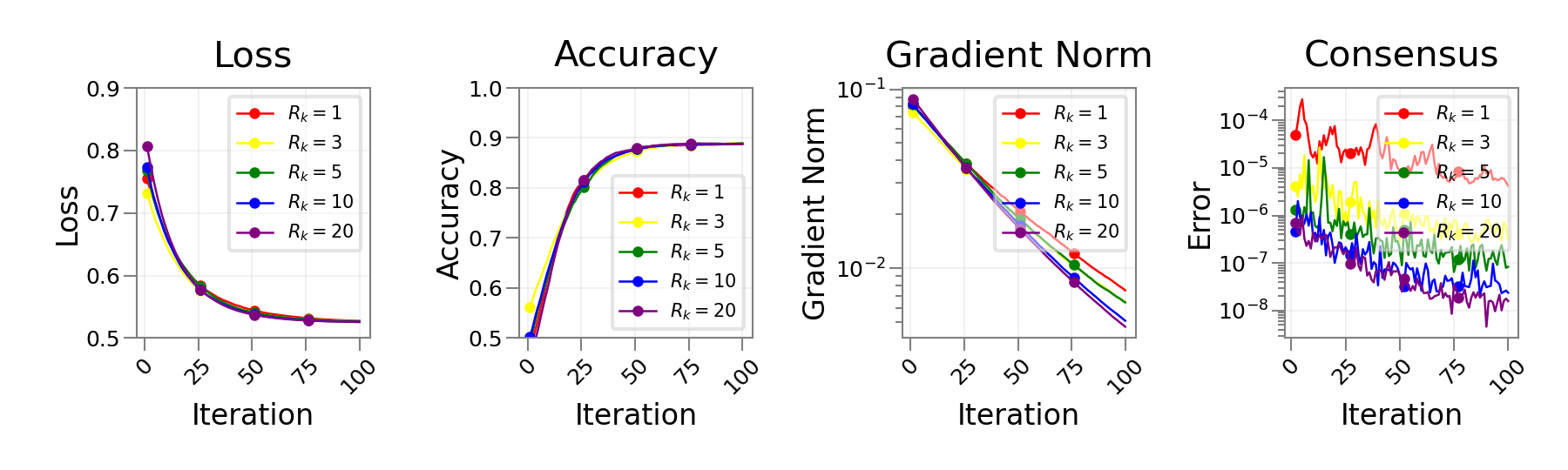
Figure A1: Effect of communication rounds $R_{k}$ in logistic regression with synthetic data

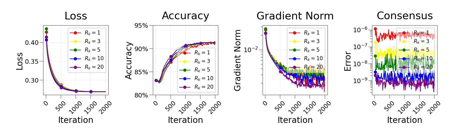
Figure A2: Effect of communication rounds $R_{k}$ in logistic regression with real data

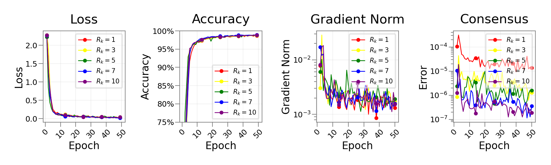
Figure A3: Effect of communication rounds $R_{k}$ in MNIST training

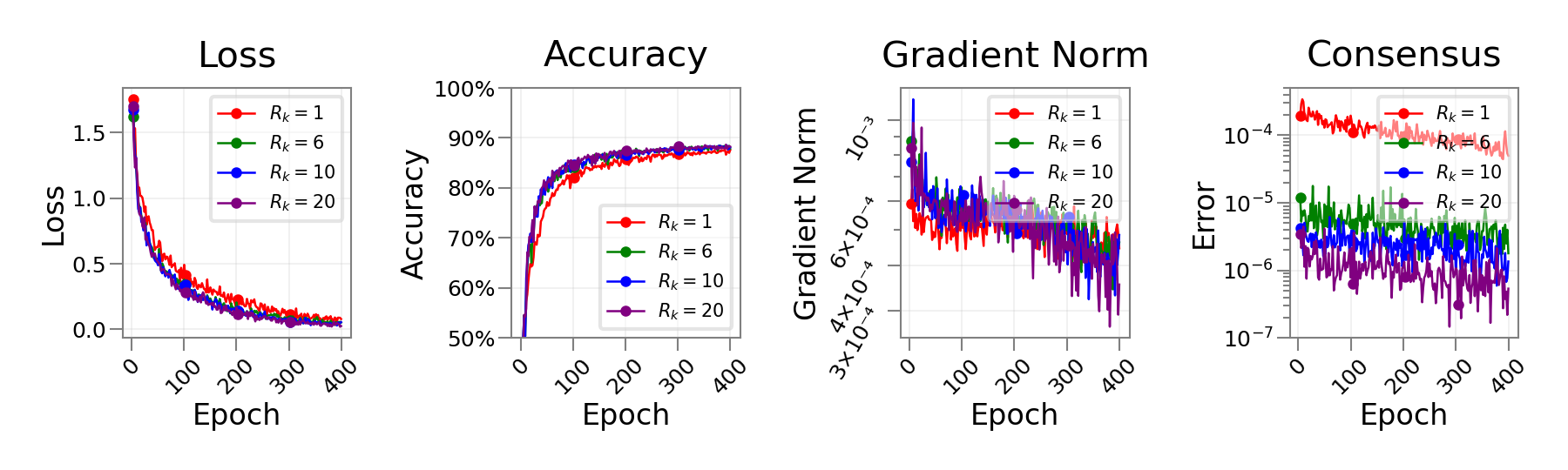
Figure A4: Effect of communication rounds $R_{k}$ in CIFAR-10 training

We defined the following metric to indicate the consensus error among all nodes:

$$e^{(k)}:=\sqrt{\frac{1}{d}\sum_{j=1}^{d}\Big(\frac{1}{n}\sum_{i=1}^{n}(x^{(k)}_{i,j}-\bar{x}^{(k)}_{j})^{2}\Big)^{2}},$$

where $\bar{x}_{j}^{(k)}:=\frac{1}{n}\sum_{i=1}^{n}x_{i,j}^{(k)}$. It can be noticed that the consensus error decreases as the rounds of inner communications increase, but not linearly. The contribution of the rounds of communications to error reduction become less obvious as the rounds increase. And for most non-convex problems, the consensus error is not decisive.

E.6 Supplementary Experiments: Comparison with Push-DIGing on Real Dataset

To further illustrate the effectiveness of our algorithm compared with Push-DIGing, we also conducted experiments of logistic regression on real dataset for comparison. The other settings were identical to those in Section 5.1, while the learning rate was set as $0.01$ for the convergence on real dataset. The results are demonstrated in Figure A5. And the conclusion is the same as in Section 5.1.

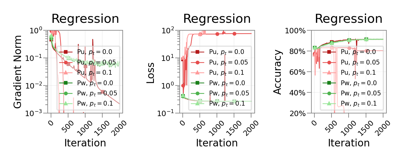
Figure A5: Comparison with Push-DIGing on real dataset

E.7 Supplementary Experiments: Performances on Different Topologies

To examine the effectiveness of our algorithms, we further conducted experiments on different topologies.

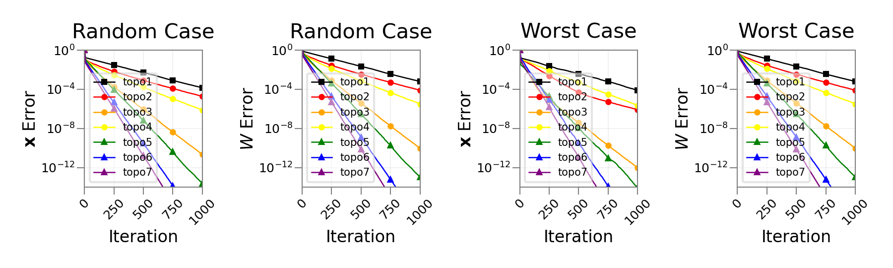
Figure A6: Consensus problems on different topologies

Figure A6 shows the performance of Algorithm 2 on different topologies. The number of nodes was $20$, and the seven topologies we chose were respectively: topo 1, ring topo with disconnection rate $0.2$; topo 2, fixed latent topo of sparsity $0.2$, with disconnection rate $0.2$; topo 3, fixed latent topo of sparsity $0.3$, with disconnection rate $0.2$; topo 4, fixed latent topo of sparsity $0.3$, with disconnection rate $0.4$; topo 5, random topo with connection rate $0.1$; topo 6, random topo with connection rate $0.2$; topo 7, random topo with connection rate $0.3$. For the data to be averaged, we considered two cases. The one used randomly generated data, while the other generated $n-1$ data randomly, but the last one significantly far from the cluster of the other nodes, which was to some degree a worst case. The metric to measure error of ${\mathbf{x}}$ is defined in 25, and we were also interested in the error of $W^{(k)}$, namely $\|W^{(k)}-E_{n}\|_{F}$.

Based on the results, we can draw two main conclusions: Algorithm 2 is robust dealing with different cases to be averaged, as it performed similarly in random and worst cases. Besides, purely random topologies own better convergence properties than topologies with a fixed latent network, as purely random topologies may have a smaller $B$ or larger $\eta$ defined in Proposition 1.

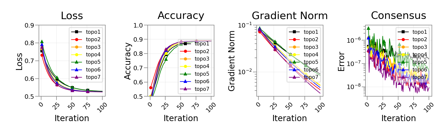
Figure A7: Logistic regression with synthetic data on different topologies

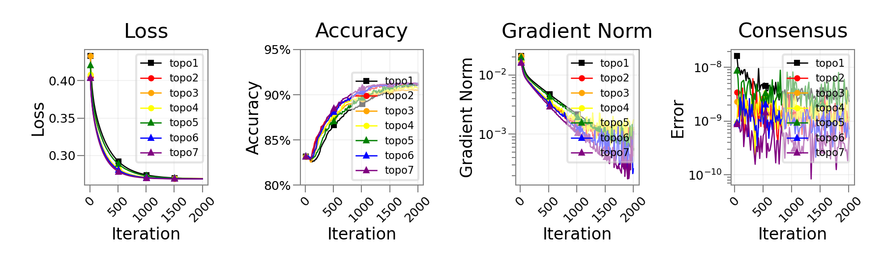
Figure A8: Logistic regression with real data on different topologies

Figure A7 and A8 show the results of Algorithm 3 on logistic regression problem using synthetic data and real data respectively. The seven topologies used for them were identical to those in Figure A6. The inner communication rounds $R_{k}$ were always $10$. Learning rates were $0.1$ for synthetic dataset and $0.01$ for real dataset. Consistent with the former experiments, topologies owning a better convergence property led to a smaller consensus error. But on the other hand, a rough accuracy of consensus is sufficient for non-convex problems, when better consensus brings no significant benefits.

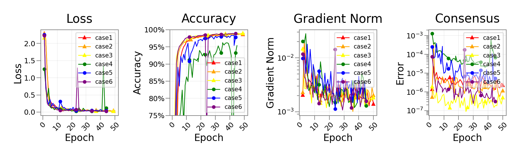
Figure A9: MNIST training on different topologies

Figure A9 shows the results of Algorithm 3 on MNIST training. Learning rate was set as $0.1$. There were six cases which we considered: case1, random data distribution on ring latent topology; case2, random data distribution on fixed latent topology; case3, random data distribution on random topologies; case 4, label-based distribution on ring latent topology; case5, label-based distribution on fixed latent topology; case6, label-based distribution on random topologies. Data were always distributed into ten nodes, and the two data distribution strategies can be referred to Section E.4. The three topology types used were: ring latent topology with a disconnection rate $0.2$; fixed latent topology with sparsity $0.3$ and with a disconnection rate $0.4$; random topologies with connection rate $0.3$. When allocating data by their labels, we should notice that different nodes might not own the same number of data. Hence, the process of epochs among different nodes might not be synchronous. We took the number of epochs within the slowest node as the indicator of the global number of epochs. Based on the results, we draw the conclusion that the properties of topologies and the distribution strategies of dataset play a more important role in the convergence of the whole problem than the inner communication rounds. However, in fairly mild settings, Algorithm 3 is still able to show good performance without a large overhead of communication or computation.