Cloud Screening of extremal charged BTZ black hole

Abstract

We study the dynamics of a charged scalar field in the near-horizon region of an extremal charged BTZ black hole. The near-horizon geometry contains an $\mathrm{AdS}_{2}$ throat with a constant electric field, which lowers the effective mass of the scalar and can trigger a violation of the $\mathrm{AdS}_{2}$ Breitenlohner–Freedman bound. We show that this instability is resolved by the formation of a static scalar cloud supported by Schwinger pair production. The condensate backreacts on the gauge field and partially screens the electric flux, leading to a self-consistent stationary configuration.
The scalar profile is obtained analytically from the near-horizon equations and exhibits the characteristic behavior of a BF-violating mode in $\mathrm{AdS}_{2}$. We analyze the associated boundary conditions, the induced charge density, and the resulting modification of the electric field. The resulting configuration can be interpreted as an electric analogue of known magnetic hairy black hole solutions.Our results provide a concrete realization of electric screening in extremal charged black holes and clarify the role of near-horizon dynamics in shaping the infrared structure of the solution.

1 Introduction

Black holes provide a rich arena for exploring the interplay between gravity, quantum field theory, and strong-field dynamics. Although early no-hair theorems suggested that stationary black holes are uniquely characterized by a small set of global charges Israel:1967za; Ruffini:1971bza, it is now well understood that these results rely on restrictive assumptions. When such assumptions are relaxed, black holes can support nontrivial external field configurations. In particular, rotating and/or charged black holes may admit long-lived scalar or vector clouds, which can develop into fully nonlinear hairy solutions hod2013no; hod2015extremal; santos2020black; Herdeiro:2016tmi. These configurations interpolate between linearized zero modes at the threshold of instability and genuinely backreacted black hole solutions.
In asymptotically AdS spacetimes, boundary conditions play a central role in determining which configurations are physically allowed. In three dimensions, scalar fields in the BTZ geometry admit mixed (Robin) boundary conditions that preserve a well-posed variational principle while allowing nontrivial profiles to develop. In this context, stationary scalar clouds and fully backreacted hairy BTZ black holes have been shown to exist Ferreira:2017cta; dappiaggi2018superradiance. These results demonstrate that nontrivial hair can arise even in low-dimensional gravity when boundary dynamics is properly accounted for.
In this work, we investigate a distinct mechanism for scalar cloud formation, driven by electric rather than rotational effects. We focus on extremal charged BTZ black holes, whose near-horizon geometry develops an $\mathrm{AdS}_{2}\times S^{1}$ throat supported by a constant electric field Cadoni:2008mw; azeyanagi2008near. In this region, charged scalar fields experience a reduction of their effective $\mathrm{AdS}_{2}$ mass. When the electric field exceeds a critical value, the BF-bound Breitenlohner:1982bm; Breitenlohner:1982jf is violated, triggering Schwinger pair production. The resulting charged excitations backreact on the gauge field, partially screening the background electric flux and giving rise to a static scalar cloud.
From a broader perspective, this phenomenon is closely connected to the emergence of infrared criticality in holographic systems. In a wide class of charged black holes, the near-horizon geometry contains an $\mathrm{AdS}_{2}$ factor, implying that the low-energy dynamics is governed by an effective $\mathrm{CFT}_{1}$ iqbal2010quantum; faulkner2011emergent; Iqbal:2011aj. In such systems, violations of the $\mathrm{AdS}_{2}$ BF-bound signal instabilities of the infrared fixed point and the emergence of new phases. These phenomena are closely tied to the appearance of complex infrared scaling dimensions and are often associated with quantum critical behavior.
A complementary perspective arises from the study of Wilson lines and defect conformal field theories. In these systems, localized degrees of freedom undergo nontrivial renormalization-group flows, leading to screening phenomena and extended clouds around defects. Recent work has shown that Wilson lines in gauge theories can support such screening clouds through defect-localized dynamics Aharony:2022ntz; Aharony:2023amq. The gravitational setup studied here provides a geometric realization of this mechanism: the extremal charged BTZ black hole acts as a dynamical impurity, while the scalar cloud plays the role of a screening cloud that modifies the infrared structure of the theory.
Related infrared phenomena have been widely studied in the context of charged black holes and holographic response functions. In particular, analyses of low-frequency dynamics have shown that when the effective $\mathrm{AdS}_{2}$ mass violates the BF-bound, scalar operators develop complex scaling dimensions, leading to oscillatory behavior and instabilities in the infrared faulkner2011emergent; iqbal2010quantum. These effects have also been observed in studies of quasinormal modes and late-time dynamics of charged black holes Hod:2012px; Degollado:2014vsa; fontana2024quasinormal. In the present work, we show that this instability admits a nonlinear resolution in the form of a static screening cloud that backreacts on the geometry and restores stability.
The near-horizon geometry of the extremal charged BTZ black hole thus provides a clean and controlled setting in which to study the interplay between electric fields, holographic infrared dynamics, and backreacted scalar condensation. The resulting configuration may be viewed as a gravitational realization of a charged impurity or Wilson-line defect, with the scalar cloud encoding the infrared response of the system. This perspective unifies several strands of previous work and provides a concrete framework for understanding electric screening and cloud formation in low-dimensional gravity.

2 Background Geometry

We start with the following action Cadoni:2008mw:

$$I=\frac{1}{16\pi G}\int d^{3}x\sqrt{-g}\left[R+\frac{2}{\ell^{2}}-4\pi GF_{\mu\nu}F^{\mu\nu}\right].$$ (1)

A solution to a static charged BTZ black hole is given by the following metric and gauge field, respectively:

$$ds_{3}^{2}=-f(r)dt^{2}+f^{-1}(r)dr^{2}+r^{2}d\theta^{2}$$ (2)

where $f(r)$ and $F_{tr}$ are given by:

$$f(r)=-8GM+\frac{r^{2}}{\ell^{2}}-8\pi GQ^{2}\ln{\left(\frac{r}{\ell}\right)},\quad\text{and}$$ (3)

$$\quad F_{tr}=\frac{Q}{r}.$$ (4)

where by setting $f(r)=0$ we find zeros of $f(r)$, namely $r_{\pm}$, where

$$\Delta=8GM-4\pi GQ^{2}\left[1-2\ln{\left(2Q\sqrt{\pi G}\right)}\right].$$ (5)

For

$$\Delta=\begin{cases}>0,\text{two horizons}\\ =0,\text{extremal(double root)}\\ <0,\text{none}.\end{cases}$$ (6)

The temperature is then given by Hawking:1975vcx; GibbonsHawking

$$T_{h}=\frac{r_{+}}{2\pi\ell^{2}}-\frac{2GQ^{2}}{r_{+}}$$ (7)

and the entropy Hawking:1975vcx; Bekenstein

$$S=\frac{\text{perimeter}}{4G}=\frac{2\pi r_{+}}{4G}=\frac{\pi r_{+}}{2G}.$$ (8)

Extremality is then found by setting

$$f(\gamma)=0\quad\text{and}\quad f^{\prime}(\gamma)=0.$$ (9)

From $f^{\prime}(\gamma)=0$ we get

$$\gamma^{2}=4\pi GQ^{2}\ell^{2}.$$ (10)

From $f(\gamma)=0$ we find the extremal mass $M_{\rm ext}$

$$M_{\rm text}=M(\gamma)=\pi Q^{2}\left[\frac{1}{2}-\ln{\left(2Q\sqrt{\pi G}\right)}\right].$$ (11)

At extremality we have $T_{H}=0$ and $S_{\rm ext}=\frac{\pi\gamma}{2G}\neq 0$. Extremal BTZ is a zero-temp, finite entropy ”ground state”.
Shifting now to $r=\gamma+x$ for $\mid x\mid\ll\gamma$, we can write the lapse function as

$$f(\gamma+x)=\frac{2}{\ell^{2}}x^{2}-8G\Delta M+\mathcal{O}(x^{3}),$$ (12)

which is the lapse function for near-horizon, near-extremal limit and

$$F_{tx}=\frac{1}{2\sqrt{\pi G}\ell}+\mathcal{O}(x).$$ (13)

where at horizon, $F_{tx}$ becomes a constant, the throat sees a uniform electric field.
The near-horizon, near-extremal metric of the charged BTZ black hole will be

$$\begin{split}ds^{2}=&-\left(\frac{2}{\ell^{2}}x^{2}-8G\Delta M\right)dt^{2}\\ &+\left(\frac{2}{\ell^{2}}x^{2}-8G\Delta M\right)^{-1}dx^{2}\\ &+\gamma^{2}d\theta^{2}\end{split}$$ (14)

and

$$F_{tx}=\frac{1}{2\sqrt{\pi G}\ell}$$ (15)

where

$$\begin{split}\Delta M&=M-M(\gamma)\\ &M-\pi Q^{2}\left[\frac{1}{2}-\ln{\left(2Q\sqrt{\pi G}\right)}\right].\end{split}$$ (16)

where $\Delta M$ is the mass above extremality As for now we will only work with extremal metric.Taking $\Delta M\to 0$ we find the extremal metric to be:

$$\begin{split}ds^{2}=&-\left(\frac{2}{\ell^{2}}x^{2}\right)dt^{2}\\ &+\left(\frac{2}{\ell^{2}}x^{2}\right)^{-1}dx^{2}\\ &+\gamma^{2}d\theta^{2}.\end{split}$$ (17)

The $(t,x)$-part is the $\rm Ads_{2}$ in the Rindler-like coordinates with radius $R_{A}^{2}=\frac{\ell^{2}}{2}$ and the circle $S^{1}$ has a fixed radius $\gamma=2\sqrt{\pi G}Q\ell$. Under dimensional reduction to $\rm 2D$, this fixed radius is a constant dilaton.
At extremality we have double zeros, giving us a quadratic throat potential $x^{2}$. The circle stays rigid ($\gamma=\rm const.$) in the throat, a constant dilaton reduction. The electric field is constant at horizon, a uniform background electric field $E$ in $\rm AdS_{2}$.
Scalar cloud formation around four-dimensional black holes has been extensively studied, particularly in the context of superradiant instabilities of rotating or charged geometries. Notable examples include stationary scalar configurations around Kerr–Newman and Reissner–Nordström black holes, as well as boson-star–like solutions supported by gravitational and electromagnetic interactions Hod:2012px; hod2015extremal; Herdeiro:2014goa. In these systems, scalar clouds typically arise from superradiant amplification and are sustained by a balance between rotation, charge, and boundary conditions.
The mechanism explored in the present work is qualitatively different. Here, the instability originates from the near-horizon $\mathrm{AdS}_{2}$ region of an extremal charged black hole, where violation of the BF bound leads to Schwinger pair production and the formation of a screening cloud. This provides a controlled setting in which black-hole hair emerges from near-horizon dynamics rather than from global superradiant amplification.
More broadly, the question of whether black holes can support nontrivial external fields has a long history. Early no-hair theorems established the uniqueness of stationary black holes under restrictive assumptions Israel:1967za; Ruffini:1971bza, suggesting that classical black holes are fully characterized by global charges. Subsequent work, however, demonstrated that these assumptions can be relaxed, and that black holes may support nontrivial scalar or vector configurations in a variety of settings, including asymptotically flat spacetimes Volkov:1998cc; Volkov:2016ehx and rotating geometries with massive vector hair Herdeiro:2016tmi. The present work fits naturally into this broader context. Rather than relying on self-interactions or rotation, the scalar cloud studied here arises dynamically from the near-horizon $\mathrm{AdS}_{2}$ region of an extremal charged black hole. The resulting configuration may be viewed as a controlled realization of hair formation driven by infrared physics, complementing earlier constructions while remaining fully consistent with the underlying gravitational dynamics.
Related phenomena have also been discussed in the context of dynamical signatures of massive fields around black holes, such as long-lived oscillatory tails and gravitational-wave imprints Degollado:2014vsa. Scalar hair and boson-star–like configurations have likewise been studied in three-dimensional gravity, particularly in asymptotically $\mathrm{AdS}_{3}$ spacetimes. Well known examples include black holes with scalar hair supported by self-interactions or nontrivial boundary conditions, as well as solitonic and boson-star solutions Henneaux:2002wm; Martinez:2004nb. In contrast, the scalar cloud studied here emerges dynamically from the near-horizon $\mathrm{AdS}_{2}$ region of an extremal charged BTZ black hole and is driven by a Schwinger instability rather than by self-interaction or global boundary conditions. This provides a controlled effective description in which hair formation is governed by near-horizon physics while remaining fully consistent with the global three-dimensional geometry.

3 Klein-Gordon equation

We consider a minimally coupled, charged scalar field $\Phi$ with mass $m$ and charge $q$ described by the action

$$S=\int d^{3}x\sqrt{-g}\left(-\frac{1}{2}D_{\mu}\Phi^{*}D^{\mu}\Phi-\frac{1}{2}m^{2}\Phi^{*}\Phi\right),$$ (18)

where $D_{\mu}=\nabla_{\mu}-iqA_{\mu}$ is the gauge-covariant derivative. The field $\Phi$ satisfies the Klein–Gordon equation:

$$\left(\nabla_{\mu}-iqA_{\mu}\right)\left(\nabla^{\mu}-iqA^{\mu}\right)\Phi-m^{2}\Phi=0.$$ (19)

which can also be written as

$$\frac{1}{\sqrt{-g}}D_{\mu}\left(\sqrt{-g}g^{\mu\nu}D_{\nu}\right)-m^{2}\Phi=0$$ (20)

where $D_{\mu}=\partial_{\mu}-iqA_{\mu}$. We solve this equation using separation of variables:

$$\Phi(t,x,\phi)=e^{-i\omega t}H_{L}(\theta)R(x),$$ (21)

where $H_{L}(\phi)$ is the eigenfunction of the angular Laplacian on $S^{1}$, satisfying $\nabla^{2}_{\perp}H_{L}=-L^{2}H_{L}$. The action of $D_{\mu}$ on $\Phi(t,x,\theta)$ for each component is given by:

$$\begin{split}D_{t}\Phi(t,x,\theta)&=-i\left(\omega+qEx\right)\phi(t,x,\theta)\\ D_{x}\Phi(t.x,\theta)&=\partial_{x}R(x)e^{-i\omega t}e^{iL\theta}\\ D_{\theta}\Phi(t,x,\theta)&=iL\,e^{-i\omega t}e^{iL\theta}R(x).\end{split}$$ (22)

and the action of $D^{\mu}\Phi(t,x,\theta)$ on each component is given by:

$$\begin{split}D^{t}\Phi(t,x,\theta)&=g^{tt}D_{t}\Phi=-\frac{\ell^{2}}{2x^{2}}D_{t}\Phi\\ D^{x}\Phi(t,x,\theta)&=g^{xx}D_{x}\Phi=\frac{2x^{2}}{\ell^{2}}D_{x}\Phi\\ D^{\theta}\Phi(t,x,\theta)&=\frac{1}{\gamma^{2}}D_{\theta}\Phi.\end{split}$$ (23)

In the following we will write components of Klein-Gordon equation:

• Time component:

  $$\begin{split}\frac{1}{\sqrt{-g}}D_{t}\left(\sqrt{-g}g^{tt}D_{t}\right)=\frac{\ell^{2}}{2x^{2}}\left(\omega+qEx\right)^{2}\Phi\end{split}$$ (24)

• Radial Component:

  $$\begin{split}&\frac{1}{\sqrt{-g}}D_{x}\left(\sqrt{-g}g^{xx}D_{x}\right)\\ &=e^{-i\omega t}e^{iL\theta}\left(\frac{4x}{\ell^{2}}R^{\prime}(x)+\frac{2x^{2}}{\ell^{2}}R^{\prime\prime}(x)\right)\end{split}$$ (25)

• Angular component:

  $$\begin{split}\frac{1}{\sqrt{-g}}D_{\theta}\left(\sqrt{-g}g^{\theta\theta}D_{\theta}\right)=-\frac{L^{2}}{\gamma^{2}}\Phi\end{split}$$ (26)

• Mass term:

  $$-m^{2}\Phi$$ (27)

Finally we can write the full radial equation as:

$$x^{2}R^{\prime\prime}(x)+2xR^{\prime}(x)+\left[\frac{\ell^{4}}{4x^{2}}\bigl(\omega+qEx\bigr)^{2}-\frac{\ell^{2}}{2}\left(m^{2}+\frac{L^{2}}{\gamma^{2}}\right)\right]R(x)=0.$$ (28)

Which we write as

$$R^{\prime\prime}(x)+\frac{2}{x}R^{\prime}(x)+\left[\frac{A}{x^{4}}+\frac{B}{x^{3}}+\frac{C}{x^{2}}\right]R(x)=0,$$ (29)

where $A,B,$ and $C$ are given by:

$$A =\frac{\ell^{4}\omega^{2}}{4}$$ (30)

$$B =\frac{\ell^{4}\omega qE}{2}$$ (31)

$$C =\frac{\ell^{4}q^{2}E^{2}}{4}-\frac{\ell^{2}}{2}\left(m^{2}+\frac{L^{2}}{\gamma^{2}}\right)$$ (32)

We use the following coordinate transformation

$$z=\frac{ik}{x},$$ (33)

From which we find that:

$$\frac{dz}{dx} =-\frac{z^{2}}{k}$$ (34)

$$R^{\prime}(x) =\frac{dR}{dz}\frac{dz}{dx}=-\frac{z^{2}}{k}R^{\prime}(z)$$ (35)

$$R^{\prime\prime}(x) =\frac{d}{dz}\left(-\frac{z^{2}}{k}R^{\prime}(z)\right)=\frac{z^{4}}{k^{2}}R^{\prime\prime}(z)+\frac{2z^{3}}{k^{2}}R^{\prime}(z).$$ (36)

Substituting eqs.(34) into the (29) we can write

$$R^{\prime\prime}(z)+\left[\frac{A}{k^{2}}+\frac{B}{k}\frac{1}{z}+\frac{C}{z^{2}}\right]R(z)=0,$$ (37)

which we will math with Whittaker equation

$$\partial_{z}^{2}R(z)+\left[-\frac{1}{4}+\frac{\kappa}{z}+\frac{1/4-\mu^{2}}{z^{2}}\right]R(z)=0.$$ (38)

We can write $\kappa$ and $\mu$ coefficients in temrs of $A,B$ and $C$ coefficients (30) and we find:

$$k =i\ell^{2}\omega$$ (39)

$$\kappa =-i\frac{\ell^{2}qE}{2}$$ (40)

$$\mu^{2} =\frac{1}{4}-C.$$ (41)

From these parameters, we can find that Schwinger pair production is on when $\mu<0$ or $C>\frac{1}{4}$ from which we find the critical electric field when Schwinger pair production happens.

$$E_{\rm crit}=\frac{1}{\mid q\mid\ell}\sqrt{1+2\ell^{2}\left(m^{2}+\frac{L^{2}}{\gamma^{2}}\right)}$$ (42)

A general solution of the radial equation (28) is given by:

$$R(x)=C_{1}M_{\kappa,\mu}\left(\frac{k}{x}\right)+C_{2}W_{\kappa,\mu}\left(\frac{k}{x}\right)$$ (43)

3.1 IR asymptotics (horizon)

Now we impose boundary conditions and for the IR we have. The large $\mid z\mid(x\to 0)$ horizon of $W$ and $M$ functions are given by:

$$\begin{split}&W_{\kappa,\mu}(z)\sim\exp\!\left(-\frac{z}{2}\right)z^{\kappa}\\ &W_{\kappa,\mu}\!\left(\frac{k}{x}\right)\sim\exp\!\left(-\frac{k}{2x}\right)\left(\frac{k}{x}\right)^{\kappa}.\end{split}$$ (44)

$$\begin{split}&M_{\kappa,\mu}(z)\sim{}\frac{\Gamma(1+2\mu)}{\Gamma\!\left(\tfrac{1}{2}+\mu-\kappa\right)}\exp\!\left(+\frac{z}{2}\right)z^{-\kappa}\\ &+\frac{\Gamma(1+2\mu)}{\Gamma\!\left(\tfrac{1}{2}+\mu+\kappa\right)}\exp\!\left(-\frac{z}{2}\right)z^{\kappa}\end{split}$$ (45)

$$\begin{split}M_{\kappa,\mu}\!\left(\frac{k}{x}\right)&\sim\frac{\Gamma(1+2\mu)}{\Gamma\!\left(\tfrac{1}{2}+\mu-\kappa\right)}\exp\!\left(+\frac{k}{2x}\right)\left(\frac{k}{x}\right)^{-\kappa}\\ &+\frac{\Gamma(1+2\mu)}{\Gamma\!\left(\tfrac{1}{2}+\mu+\kappa\right)}\exp\!\left(-\frac{k}{2x}\right)\left(\frac{k}{x}\right)^{\kappa}.\end{split}$$ (46)

Then for $k=i\sqrt{2}\ell^{2}\omega$, the two phases $\exp{\left(\mp\frac{k}{2x}\right)}$ are oscillatory and the infalling IR mode is the one proportional to $\exp{\left(-\frac{ik}{2x}\right)}$. Therefore from it IR boundary condition we have

$$R_{\rm IR}(x)\propto W_{\kappa,\mu}\!\left(\frac{k}{x}\right)\sim\exp\!\left(-\frac{k}{2x}\right)\left(\frac{k}{x}\right)^{\kappa},\quad x\to 0.$$ (47)

3.2 UV Asymptotics ($\mathrm{AdS}_{2}$ Boundary)

We expand $W_{\kappa,\mu}$ for small $z$:

$$\begin{split}W_{\kappa,\mu}(z)\;=\;&\frac{\Gamma(2\mu)}{\Gamma\!\left(\tfrac{1}{2}+\mu-\kappa\right)}\,z^{\frac{1}{2}-\mu}\\ &+\frac{\Gamma(-2\mu)}{\Gamma\!\left(\tfrac{1}{2}-\mu-\kappa\right)}\,z^{\frac{1}{2}+\mu}+\mathcal{O}\!\left(z^{\frac{3}{2}\pm\mu}\right).\end{split}$$ (48)

and in terms of our $x$-coordinate we have

$$\begin{split}R_{\rm UV}(x)=C_{1}\bigg[&\underbrace{\frac{\Gamma(2\mu)}{\Gamma\!\left(\tfrac{1}{2}+\mu-\kappa\right)}k^{\frac{1}{2}-\mu}}_{A_{-}(\kappa,\mu)}\,x^{-\frac{1}{2}+\mu}\\ &+\underbrace{\frac{\Gamma(-2\mu)}{\Gamma\!\left(\tfrac{1}{2}-\mu-\kappa\right)}k^{\frac{1}{2}+\mu}}_{A_{+}(\kappa,\mu)}\,x^{-\frac{1}{2}-\mu}+\cdots\bigg].\end{split}$$ (49)

Here, both branches scale as $x^{-1/2}$. For the screening cloud boundary condition we eliminate one branch (for “no incoming from the boundary”) which happens when a denominator gamma hits a pole:

$$\frac{1}{2}+\mu-\kappa=-n,\qquad n\in\mathbb{Z}_{\geq 0}.$$ (50)

In the BF-violating regime the near-boundary scaling exponent becomes imaginary, $\mu=ib,b\in\mathbb{R}$. In this case the UV pole condition (50) cannot be satisfied: both $\mu$ and $\kappa$ are purely imaginary, so the combination $\tfrac{1}{2}+\mu-\kappa$ never lies on the negative real axis.
Therefore the slow-falloff coefficient $A_{-}$ cannot be removed by imposing a standard UV Dirichlet-type boundary condition. Instead, one must impose a mixed (double-trace) boundary condition, which fixes the ratio $A_{-}/A_{+}$. This is the correct holographic boundary condition for the BF-violating $\mathrm{AdS}_{2}$ throat.
When the electric field exceeds the critical value $E_{\rm crit}$, the effective mass of the scalar in the $\mathrm{AdS}_{2}$ region drops below the BF bound. The scaling dimensions become complex,

$$\Delta_{\pm}=\frac{1}{2}+\mu=\frac{1}{2}\pm ib,$$ (51)

and the UV wavefunctions become oscillatory. The interpretation of the BF bound in $\mathrm{AdS}_{2}$ Breitenlohner:1982bm; Breitenlohner:1982jf differs in an important way from higher-dimensional cases. In $\rm AdS_{d+1}$ with $d>1$, the BF bound coincides with the point at which the operator in the alternative quantization reaches the unitarity bound. In contrast, in $\rm AdS_{2}$ there is no independent unitarity bound of this type. Instead, when the BF bound is saturated, the elementary operator acquires scaling dimension $\Delta=1/2$, and it is the associated bilinear operator that becomes marginal. This feature underlies the emergence of nontrivial infrared dynamics and has been extensively discussed in the context of holographic quantum criticality and semi-local quantum liquids iqbal2010quantum; faulkner2011emergent; Iqbal:2011aj. From this perspective, the instability observed here should be understood as a dynamical realization of this general mechanism. The violation of the $\rm AdS_{2}$ BF bound triggers Schwinger pair production and leads to the formation of a screening cloud, providing a concrete gravitational realization of emergent infrared physics. Related phenomena have also been discussed in the context of scalar clouds and long-lived excitations around black holes Hod:2012px; hod2015extremal; Herdeiro:2014goa; Degollado:2014vsa.
This signals the onset of Schwinger pair production: the electric field is strong enough to pull virtual charged pairs out of the vacuum. The negatively charged particle accelerates toward the horizon, while the positively charged one is driven outward, producing an outgoing flux in the UV. Geometrically, the throat behaves like a capacitor at its breakdown voltage: for $E>E_{\rm crit}$ virtual pairs continually appear and populate the throat, forming a diffuse charged cloud.

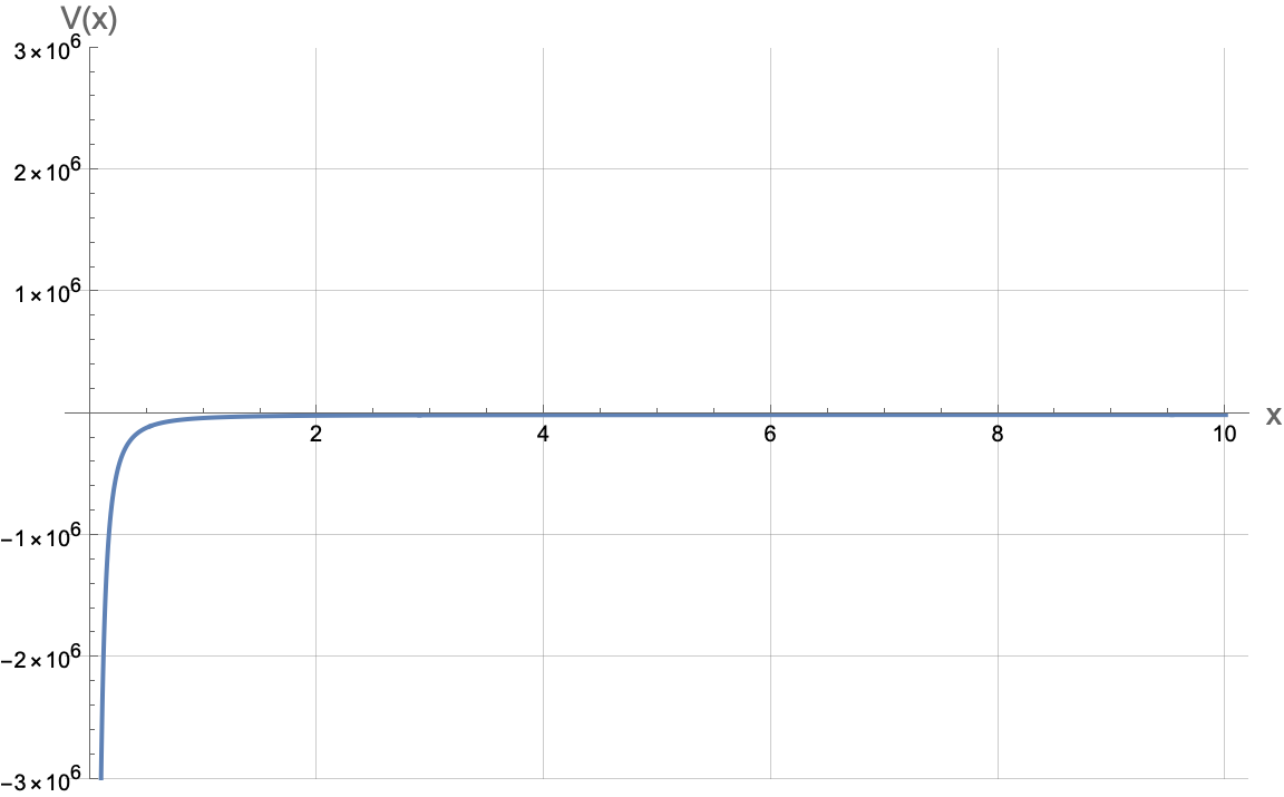
Figure 1: Effective potential $V_{\text{eff}}(x)$ as a function of the radial coordinate $x$.

The effective potential term that we plot is given by:

$$\begin{split}\mathcal{V}(x)=&\underbrace{\Bigg[\,-\frac{\ell^{4}(qE)^{2}}{4}+\frac{\ell^{2}}{2}\,m_{\mathrm{eff}}^{2}\,\Bigg]}_{\text{constant (BF part)}}\\ &-\underbrace{\frac{\ell^{4}\,\omega\,qE}{2}\,\frac{1}{x}}_{\text{Coulomb tilt}}-\underbrace{\frac{\ell^{4}\,\omega^{2}}{4}\,\frac{1}{x^{2}}}_{\text{near-horizon term}}\,.\end{split}$$ (52)

• The constant term decides global BF–bound violation.

• The $1/x$ term is a “tilt” from time dependence and charge coupling $(qE\omega)$.

• The $1/x^{2}$ term dominates near the horizon and is attractive (negative).

At the near horizon ($x\!\to\!0$), $\mathcal{V}(x)<0$ and the $-A/x^{2}$ term dominates, acting as an attractive well that supports oscillatory IR solutions. In the intermediate region the $1/x^{2}$ term decays, the $1/x$ term becomes important, and the point where $\mathcal{V}(x)=0$ plays the role of a classical turning point or barrier. Beyond this point the solutions transition from oscillatory to exponentiallydecaying as one moves toward the $\mathrm{AdS}_{2}$ boundary. For large $x$ the constant term dominates, $\mathcal{V}(x)>0$, and the cloud cannot extend any further into the UV.

4 Including Boundary Terms

In this section, we will explain why including boundary terms is necessary. As metioned in Ferreira:2017cta; Dappiaggi:2017pbe, the AdS timelike (conformal) boundary yields the possibility of placing material sources (or absorbers) on the boundary and that is achieved by considering mixed (Robin) boundary conditions Ferreira:2017cta. The appearance of mixed (Robin) boundary conditions and the associateddouble-trace renormalization-group flow has a well-established interpretation in the context of AdS/CFT. Such boundary conditions arise when multi-trace operators are added to the dual theory, and their role in defining consistent variational principles and holographic RG flows has been extensively studied Witten:2001ua; Berkooz:2002ug; Hartman:2006dy; das2013double; Aharony:2015afa.
First, We switch from $x$ to a radial variable $r$ that vanishes at the $\rm AdS_{2}$ boundary

$$r\equiv\frac{1}{x}$$ (53)

where $r\to 0$ now represents the boundary and $r\to\infty$ represents the horizon. The UV expression now (49) written in terms of $r-$coordinate (53) is now given by:

$$R(r)=A_{-}r^{\Delta_{-}}+A_{+}r^{\Delta+}+\dots,$$ (54)

where the scaling dimension $\Delta_{\pm}$ is given by (51). $A_{-}$ multiplies the less decaying mode (more singular) $r^{\Delta_{-}}$, while $A_{+}$ multiplies more decaying (less singular) mode $r^{\Delta_{+}}$. We now also introduce a small radial cuttoff at $r=r_{0}$ representing the UV wall. Reducing over the circle $S^{1}$ and focusing on a singular harmoinc $L$, our scalar field now lives on $\rm AdS_{2}$ with effecitve mass $m_{\rm eff}$ and with bulk action given by:

$$S_{\rm bulk}=\int d^{2}x\sqrt{-g_{(2)}}\left(-\mid D_{\mu}\ \Phi\mid^{2}-m_{\rm eff}^{2}\mid\Phi\mid^{2}\right).$$ (55)

Varying the action and integrating by parts we find

$$\delta S_{\rm bulk}=\left(\text{EOM terms}\right)+\delta S_{\rm bdy}^{\rm bulk}.$$ (56)

The boundary variation of the bulk action takes the standard form

$$\delta S_{\rm bdy}^{\rm bulk}=\int_{r=r_{0}}dt\sqrt{-\gamma}\,n^{r}\left((D_{r}\Phi)^{*}\,\delta\Phi+\text{c.c.}\right),$$ (57)

to make the variational problem well-posed (without adding further boundary terms) one must hold fixed one of the two asymptotic coefficients at the cutoff. In the present normalization the boundary variation takes the form

$$\delta S_{\rm bulk}\Big|_{r=r_{0}}\;\propto\;(1-2\mu)\,r_{0}^{-2\mu}\,\Big(A_{-}^{*}\,\delta A_{-}+\text{c.c.}\Big)\;+\;\cdots,$$ (58)

where the ellipsis denotes terms subleading in $r_{0}$ and/or proportional to $\delta A_{+}$. A standard (Dirichlet-type) variational principle is obtained by fixing $A_{-}$ at the boundary, i.e.

$$\delta A_{-}(t)=0\qquad\text{at }r=r_{0}.$$ (59)

In holographic language this means that $A_{-}$ plays the role of the source, while $A_{+}$ is determined dynamically and encodes the response (vev). Setting $A_{-}=0$ corresponds to the special case of turning off the source; it is a choice of state, not the definition of the variational principle.
In this standard quantization the dual operator has scaling dimension $\Delta_{+}=\frac{1}{2}+\mu$. Since the bulk field $\Phi$ is charged under the bulk $U(1)$, strictly local gauge-invariant defect operators are built from neutral composites; the simplest one is the bilinear

$$\mathcal{O}_{\rm std}\sim\Phi^{*}\Phi,\qquad\hat{\Delta}_{+}=2\Delta_{+}=1+2\mu.$$ (60)

Within the unitary window $0<\mu<\frac{1}{2}$ this operator is irrelevant in the standard quantization, so adding it as a local boundary interaction does not generate a nontrivial IR flow. In the decoupling limit $q\to 0$ (no electric coupling) one has $\mu\to\frac{1}{2}$ for a massless scalar, so the bilinear has $\hat{\Delta}_{+}=2$ as expected for the ordinary ${\rm AdS}_{2}/{\rm CFT}_{1}$ vacuum with no defect.
Following Aharony:2015afa; Aharony:2022ntz; Aharony:2023amq, we now add a local boundary counterterm at the cutoff surface $r=r_{0}$,

$$S_{\rm bdy}^{(1)}\;=\;-\frac{1-2\mu}{2}\int_{r=r_{0}}dt\sqrt{-\gamma}\,|\Phi|^{2}.$$ (61)

This term does not represent a deformation of the theory, but rather a necessary counterterm that renders the variational problem finite and allows for an alternative choice of quantization in the AdS₂ throat.

Varying $S_{\rm bdy}^{(1)}$ and combining it with the boundary variation of the bulk action, the leading divergent contribution proportional to $A_{-}^{*}\delta A_{-}$ cancels. For $0<\mu<\frac{1}{2}$ and $r_{0}\to 0$, the remaining boundary variation is dominated by the cross term

$$\delta S_{\rm bdy}\;\sim\;A_{+}^{*}\,\delta A_{-}+A_{-}^{*}\,\delta A_{+}.$$ (62)

A well-posed variational principle is therefore obtained by fixing $A_{+}$ at the boundary, i.e. by imposing $\delta A_{+}=0$. This defines the alternative quantization in the AdS₂ throat, in which $A_{+}$ plays the role of the source while $A_{-}$ is dynamical. Setting $A_{+}=0$ corresponds to turning off the source in this quantization.

In the alternative quantization the near-boundary behavior

$$\Phi\sim A_{-}\,r^{\Delta_{-}},\qquad\Delta_{-}=\frac{1}{2}-\mu,$$ (63)

is interpreted as the expectation value of the dual operator. The lowest strictly local gauge-invariant operator on the defect is again the bilinear $\Phi^{*}\Phi$, now with scaling dimension

$$\hat{\Delta}_{\rm alt}=1-2\mu.$$ (64)

Both the standard and alternative quantizations are unitary within the window $0<\mu<\frac{1}{2}$, but they correspond to distinct defect CFTs with different operator spectra, in direct analogy with Aharony:2023amq.
We now perturb the alternative defect CFT by the relevant operator $|\Phi|^{2}$. In AdS language this corresponds to a double-trace deformation, implemented by adding a second boundary term

$$S_{\rm bdy}^{(2)}\;=\;-f_{0}\int_{r=r_{0}}dt\sqrt{-\gamma}\,r_{0}^{2\mu}\,|\Phi|^{2}.$$ (65)

At leading order in small $r_{0}$, the total boundary variation becomes

$$\delta\!\left(S_{\rm bulk}+S_{\rm bdy}^{(1)}+S_{\rm bdy}^{(2)}\right)\simeq\int d\omega\,\Big[2\mu\,(A_{+}^{*}\delta A_{-}+A_{-}^{*}\delta A_{+})+f_{0}\,(A_{-}^{*}\delta A_{-}+\text{c.c.})\Big].$$ (66)

A well-posed variational principle is obtained by imposing a mixed (Robin) boundary condition of the form

$$A_{+}\;=\;f(r_{0})\,A_{-},$$ (67)

where $f(r_{0})$ is the dimensionless double-trace coupling defined at the cutoff scale. Requiring the total variation to vanish yields the renormalization-group equation

$$\beta_{f}\;\equiv\;\frac{df}{d\log r_{0}}\;=\;-2\mu\,f+f^{2}.$$ (68)

For $0<\mu<\frac{1}{2}$ this flow has two fixed points,

$$f_{*}=0,\qquad f_{*}=2\mu,$$ (69)

corresponding respectively to the alternative (UV) and standard (IR) quantizations. We emphasize that this double-trace RG flow applies when $\mu$ is real ($0<\mu<\frac{1}{2}$); in the BF-violating regime $\mu=ib$ the scaling dimensions are complex and the appropriate boundary condition is instead fixed by self-adjointness and flux conservation, rather than by an RG fixed point.
It is useful to interpret the above boundary structure from the perspective of worldline effective field theory. In this language, a heavy charged object is represented by a Wilson line operator coupled to the bulk gauge field, as developed in the effective descriptions of charged compact objects Goldberger:2004jt; Goldberger:2005cd. From this viewpoint, the extremal charged BTZ black hole acts as a static electrically charged defect, whose interaction with the bulk fields is encoded in boundary data at the $\rm AdS_{2}$ edge. The appearance of mixed (Robin) boundary conditions and the associated double-trace flow admits a natural interpretation as the dynamical dressing of this Wilson line by charged matter. In particular, the scalar cloud generated by Schwinger pair production plays the role of a screening cloud that renormalizes the effective charge of the defect. This is closely analogous to the renormalization of Wilson lines in scalar QED and related systems Aharony:2015afa; Aharony:2022ntz; Aharony:2023amq, but here realized dynamically in a curved near-horizon geometry.
From this perspective, the RG flow between the alternative and standard quantizations reflects the flow between distinct effective descriptions of the charged defect, while the onset of the BF instability signals the breakdown of the trivial Wilson line and the formation of a nonperturbative screening cloud. We now turn to the explicit realization of this picture in the subcritical and supercritical regimes.

4.1 Below the Electric BF Threshold

We now analyze the regime in which the effective $\rm AdS_{2}$ exponent

$$\mu=\sqrt{\tfrac{1}{4}-C}>0,\qquad(C<\tfrac{1}{4}),$$ (70)

is real. This corresponds to a subcritical electric field in the near-horizon region. In this case the extremal charged BTZ throat lies safely above the AdS₂ BF-bound, and the dual defect CFT₁ is unitary even without any scalar condensate. Schwinger pair production is exponentially suppressed, and no dynamical instability is present in the bulk geometry.
The scalar field therefore behaves as in an ordinary AdS₂ defect: the two independent near-boundary modes have real scaling dimensions (51) where retarded Green’s function is analytic for $\text{Im}\left(\omega\right)$, and small perturbations decay toward the horizon. The effective potential (52) also reflects this: although the $-\omega^{2}/x^{2}$ term produces the familiar attractive near-horizon well, the constant BF term is positive;

$$\mathcal{V}(x)\xrightarrow[x\to\infty]{}\mu^{2}>0,$$ (71)

and therefore prevents the existence of a normalizable static zero-mode. No static bound state can decay simultaneously at the horizon and at the $\rm AdS_{2}$ boundary.
Consequently, the only globally regular static configuration compatible with the boundary conditions is the trivial one

$$\Phi=0,\qquad A_{t}(x)=E\,x,$$ (72)

corresponding to the unperturbed extremal BTZ throat with a uniform electric field. For any choice of the double-trace coupling $f$ within the physical range $0\leq f\leq 2\mu$ both the bulk and boundary descriptions remain stable: the defect theory stays unitary, and the bulk geometry admits no nontrivial static cloud.
In particular, no screening occurs in the subcritical regime. The effective mass never approaches the BF-bound, the throat does not produce charged pairs, and the electric field remains unscreened. The emergence of a scalar cloud is therefore a genuinely supercritical phenomenon, tied to BF-bound violation and Schwinger pair production, which we analyze in the next subsection.

4.2 Beyond the Electric BF Threshold: Onset of Schwinger Cloud Condensation

We now turn to the regime in which the near-horizon electric field exceeds the critical value for charged pair creation. Equivalently, the effective $\rm Ads_{2}$ exponent becomes imaginary,

$$\mu^{2}<0\qquad\Longleftrightarrow\qquad C>\frac{1}{4},$$ (73)

and we write

$$\mu=ib,\qquad b>0.$$ (74)

In this regime the charged scalar violates the $\rm Ads_{2}$ BF bound, and the corresponding operator in the dual defect CFT₁ acquires a complex scaling dimension

$$\Delta_{\pm}=\frac{1}{2}\pm ib.$$ (75)

At the level of the naive defect $\rm CFT_{1}$, complex scaling dimensions indicate a loss of reflection positivity and hence non-unitarity. This does not signal an inconsistency of the full theory, but rather the instability of the trivial saddle. Instead of a simple power law decay, the solution becomes oscillatory. For a real scalar configuration we can choose coefficients such that $A_{+}=A_{-}^{*}$. Using $r^{-ib}=\left(e^{\ln r}\right)^{ib}$ and the complex conjugate of it, we can write the radial solution as:

$$R(r)=\mathcal{C}\sqrt{r}\cos{\left(b\log{\left(r/r_{0}\right)}+\delta\right)},$$ (76)

where we find that

$$\delta=-\frac{1}{2}\arg\left(\frac{A_{+}}{A_{-}}\right).$$ (77)

In the BF-violating regime we have Schwinger pair production. The scalar field feels an accelerating electric field, a horizon that absorbs infalling charge and a UV region that reflects outgoing charge depending on the boundary condition. The scalar solution is a wave bouncing between UV and IR but in the 1D cavity we have an interesting geometry, the coordinaate is $\ln{r}$. So the wave picks up a phase along the throat, this is the phase $\delta$, i.e. it encodes how pair-produced charges interfere as they try to climb out of the throat.

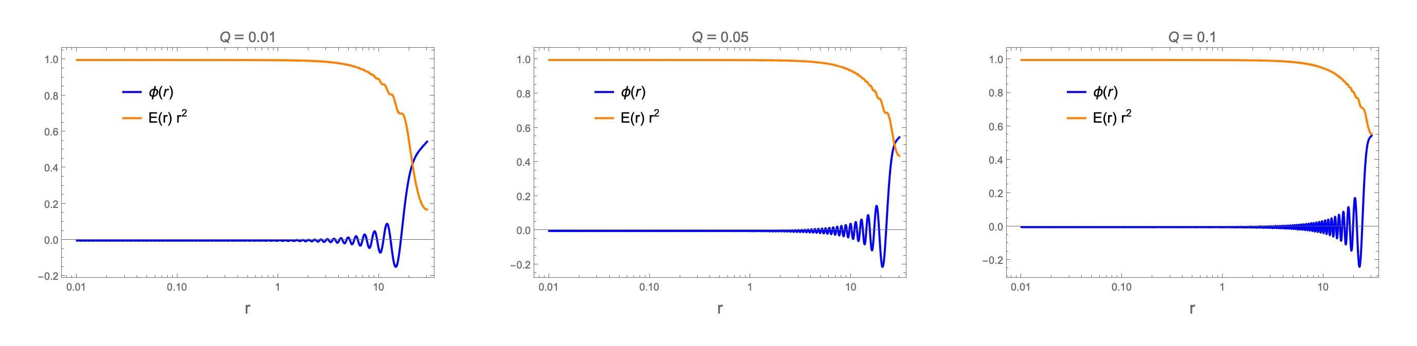
Figure 2: Radial profiles of the scalar mode $\phi(r)$ (blue) and the electric field $E(r)\,r^{2}$ (orange), obtained from the nonlinear system in the near-horizon $\mathrm{AdS}_{2}$ region of the extremal charged BTZ geometry. The horizontal axis is the Poincaré radius $r$, where $r\to 0$ corresponds to the $\mathrm{AdS}_{2}$ boundary. For visibility, the electric field is normalized by its value at a UV reference point $r_{\mathrm{UV}}$. The three panels show increasing values of the IR electric field $E_{0}$, which is proportional to the black-hole charge $Q$. Larger $E_{0}$ enhances the BF-violating instability: the scalar cloud develops a larger log-oscillatory envelope near the horizon, and the electric field exhibits stronger suppression as $r\to 0$, reflecting classical screening by the condensate. Full screening requires the one-loop quantization analysis of the defect, discussed in Sec. 6.

5 Effective Field Description and Quantization

We now develop an effective description of the charged scalar cloud in the near–horizon region. All ingredients needed for the construction, the near–extremal ${\rm AdS}_{2}$ geometry, the Whittaker solution, the BF–violating condition, the IR ingoing boundary condition and the UV mixed boundary condition—were derived in Sections 2,3 and 4. Here we simply assemble these elements into the effective $2{\rm D}$ theory that governs the dynamics of the cloud.

5.1 Effective Field Regime and Background Geometry

After dimensional reduction on the rigid circle of radius $\gamma$, the dynamics is captured by a charged complex scalar $\Phi(t,r)$ propagating in the extremal ${\rm AdS}_{2}$ throat. In Poincaré coordinates (53) where the ${\rm AdS}_{2}$ boundary lies at $r\to 0$ and the horizon at $r\to\infty$, the metric takes the form

$$ds_{(2)}^{2}=\frac{R_{A}^{2}}{r^{2}}(-dt^{2}+dr^{2}),\qquad R_{A}^{2}=\frac{\ell^{2}}{2},$$ (78)

and the electric field obtained in Sec. 2 is constant,

$$F_{tr}=E=\frac{1}{2\sqrt{\pi G}\,\ell}.$$ (79)

The reduced $2{\rm D}$ action is therefore

$$\begin{split}S_{2D}=\int d^{2}x\,\sqrt{-g_{(2)}}\,\Big[-\frac{1}{2}(\partial\mathcal{R})^{2}&-\frac{1}{2}\,\mathcal{R}^{2}(\partial\pi-qA_{\mu})^{2}-\frac{1}{2}\,m_{\rm eff}^{2}\,\mathcal{R}^{2}\Big]\\ &-\frac{1}{4g_{2}^{2}}\int d^{2}x\,\sqrt{-g_{(2)}}\,F_{\mu\nu}F^{\mu\nu}.\end{split}$$ (80)

To make contact with an effective description it is convenient to write the charged scalar in amplitude–phase variables,

$$\Phi(t,r)=\frac{1}{\sqrt{2}}\,\mathcal{R}(r)\,e^{-i\omega t+i\pi(r)}.$$ (81)

For the stationary cloud we set $\omega=0$, so $|\Phi|^{2}=\mathcal{R}^{2}/2$. In the BF-violating regime $\mu=ib$ the two independent UV falloffs combine into a log-oscillatory profile (76). The near–boundary behavior of the scalar field is governed by the exponent $\mu$ obtained in Sec. 3. The real linear combination corresponds to a static, current-free condensate and is the appropriate saddle for the screening cloud. In the supercritical (BF–violating) regime (74) the two independent UV falloffs are given by (54) and the full radial profile is the BF–violating Whittaker solution already constructed in Sec. 3.The real, stationary configuration corresponds to the real linear combination of the two Whittaker branches (cf. Sec. 3) (76), with constants fixed by the UV mixed boundary condition. This is the classical cloud that stores the charge produced by the Schwinger process.
The physical IR boundary condition derived in Sec. 3 selects the ingoing Whittaker branch, its modulus determines the coarse grained one–point function of the condensate,

$$|R_{\rm in}(r)|^{2}\propto r,$$ (82)

which we write as

$$\langle|\Phi(r)|^{2}\rangle=\frac{\mathcal{C}^{2}}{2}\,r.$$ (83)

The envelope grows toward the horizon, reflecting accumulation of low-energy charge in the $\rm AdS_{2}$ throat; global finiteness and total screened charge require the quantized analysis in Sec.6. The constant $\mathcal{C}$ is fixed by the UV boundary condition (the value of the double–trace coupling $f$ at the cutoff). The profile (83) grows toward the horizon and vanishes at the boundary, reflecting the accumulation of Schwinger–produced charges in the ${\rm AdS}_{2}$ throat.
Unlike the flat–space cloud of Aharony:2023amq, which decays as $1/r^{2}$, the near–horizon ${\rm AdS}_{2}$ background leads to a growth $\sim r$ due to the BF–violating scaling dimension $\Delta_{\pm}=\frac{1}{2}\pm ib$. This geometric effect is crucial: it is the $\rm AdS_{2}$ redshift that prevents the escape of low–frequency excitations and allows a stationary cloud to form. The coarse–grained profile (83) now serves as the semiclassical background for the effective defect theory developed in the next subsection.
The amplitude $\mathcal{C}$ is fixed by the UV mixed boundary condition (i.e. by the double-trace coupling at the cutoff). The growth toward the horizon reflects the accumulation of low-energy charge in the AdS₂ throat; the total screened charge is determined only after including backreaction and one-loop quantization.

5.2 Field Decomposition and Higgs–Goldstone Effective Action

We now use the decomposition (81) with $\mathcal{R}(x)>0$ the real amplitude and $\pi(x)$ the real phase field. The gauge symmetry

$$\Phi\to e^{iq\alpha(x)}\Phi,\qquad A_{\mu}\to A_{\mu}+\partial_{\mu}\alpha$$ (84)

acts as

$$\mathcal{R}(x)\to\mathcal{R}(x),\qquad\pi(x)\to\pi(x)+q\alpha(x).$$ (85)

Thus, $\mathcal{R}$ is gauge invariant and describes fluctuations in the magnitude of the condensate (the “Higgs” direction in field space), while $\pi$ shifts under the gauge symmetry and plays the role of the Goldstone mode. The gauge-invariant combination built from $\pi$ and $A_{\mu}$ is

$$\partial_{\mu}\pi-qA_{\mu},$$ (86)

the standard “covariant derivative of the phase”, which gives an effective mass to the gauge field once $\mathcal{R}$ acquires a nonzero background value.
After reduction on the circle and including the gauge kinetic term, the full $2\rm D$ effective action can be written in Higgs form,

$$\begin{split}S_{2D}&=-\frac{1}{4}\int d^{2}x\sqrt{-g_{(2)}^{2}}\left[(\partial\mathcal{R})^{2}+\mathcal{R}^{2}\left(\partial\pi-qA\right)^{2}+m_{\rm eff}^{2}\right]\\ &-\frac{1}{4g_{2}^{2}}\int d^{2}x\sqrt{-g_{(2)}^{2}}F_{\mu\nu}F^{\mu\nu}\end{split}$$ (87)

Varying with respect to $\mathcal{R}$, $\pi$ and $A_{\mu}$ gives the coupled saddle-point equations

$$-\mathcal{R}^{\prime\prime}(r)=\mathcal{R}\left[\pi^{\prime 2}(r)-qA_{t}^{2}(r)\right]+\frac{R_{A}^{2}}{r^{2}}m_{\rm eff}^{2}\mathcal{R},$$ (88)

$$\frac{d}{dr}\left[\mathcal{R}^{2}(r)\pi^{\prime}(r)\right]=0,$$ (89)

$$\frac{d}{dr}\left[\frac{r^{2}}{R_{A}^{2}g_{2}^{2}}A_{t}^{\prime}(r)\right]=\frac{1}{2}q^{2}\mathcal{R}A_{t}(r).$$ (90)

The coupled system obtained in Eq. (88) admits several qualitatively distinct branches. Before discussing screening, it is useful to organize the structure of solutions systematically. The Goldstone equation,

$$\partial_{r}\bigl(\mathcal{R}^{2}\pi^{\prime}\bigr)=0,$$ (91)

implies $\mathcal{R}^{2}\pi^{\prime}=C_{\pi}$ for some constant $C_{\pi}$. Regularity at both the AdS₂ boundary ($r\to 0$) and the horizon ($r\to\infty$) forces $C_{\pi}=0$, since any nonzero value produces a singular phase gradient. Thus the phase is pure gauge

$$\pi^{\prime}(r)=0,$$ (92)

and the only dynamical fields in the background are the amplitude $\mathcal{R}(r)$ and the gauge potential $A_{t}(r)$.
With $\mathcal{R}(r)=0$ identically, the Maxwell equation reduces to

$$\partial_{r}\!\left(\frac{r^{2}}{R_{A}^{2}g_{2}^{2}}A_{t}^{\prime}\right)=0,$$ (93)

whose solution is a constant Gauss flux. This branch describes the extremal AdS₂ throat supported purely by the background electric field. No scalar cloud forms and there is no screening: the electric field is constant up to the usual redshift factor $r^{2}$.
A genuine condensate requires $\mathcal{R}(r)\neq 0$. The amplitude equation becomes

$$\mathcal{R}^{\prime\prime}=-q^{2}A_{t}^{2}\mathcal{R}+\frac{R_{A}^{2}m_{\rm eff}^{2}}{r^{2}}\,\mathcal{R},$$ (94)

which admits normalizable solutions only in the BF–violating regime. In this regime the scalar oscillates logarithmically, (76) and its coarse–grained (83) grows toward the horizon.
The Maxwell equation is then sourced by $\mathcal{R}^{2}A_{t}$ and the Gauss flux is no longer constant. This is precisely the classical screening mechanism.
A nonzero solution $\mathcal{R}_{s}(r)$ represents the static scalar cloud supported in the near-horizon region by Schwinger pair production. The corresponding gauge field $A_{t}(r)$ is no longer linear in $r$; the quantity

$$\mathcal{E}(r)\equiv\frac{r^{2}}{R_{A}^{2}g_{2}^{2}}\,A_{t}^{\prime}(r),$$ (95)

monotonically decreases toward the AdS₂ boundary, reflecting the partial screening of the electric field by the condensate. The trivial and nontrivial branches, therefore correspond to the unscreened and screened phases of the system.
In practice we display both fields in terms of their radial profiles:

• the amplitude $\mathcal{R}_{s}(r)$, which grows and develops the expected log–oscillatory structure near the horizon, and

• the physical electric field $\mathcal{E}(r)$, which is constant on the trivial branch but decreases toward the boundary for the cloud branch. These plots make explicit the transition from the pure-AdS₂ electric throat to the screened configuration generated by the scalar condensate.

It is worth recalling a general AdS₂ fact that a constant electric field acts as a negative contribution to the effective AdS₂ mass of a charged scalar. In flat space this phenomenon is familiar from radial quantization of Wilson lines Kapustin:2005py. Upon rewriting the metric as $ds^{2}=r^{2}(ds^{2}_{\text{AdS}_{2}}-d\Omega_{2}^{2})$, the Coulomb field $A_{t}=e^{2}q/(4\pi r)$ becomes a constant electric field in AdS${}_{2}\times S^{2}$, and the scaling dimension satisfies Aharony:2023amq; Aharony:2022ntz

$$\frac{\Delta}{2}\!\left(\frac{\Delta}{2}-1\right)=-\,\frac{e^{4}q^{\,2}}{16\pi^{2}}.$$ (96)

Thus the electric field shifts the effective AdS₂ mass downward, potentially driving it below the BF bound. This is precisely the mechanism that appears in the charged BTZ throat: the near-horizon electric field contributes a term $-R_{A}^{4}q^{2}E^{2}$ to the effective mass, leading to the BF-violating exponent $\mu^{2}=\frac{1}{4}-C$ derived in Section 3.
Electric field creates pairs $(+q,-q)$ and $\rm AdS_{2}$ geometry traps them, kind of acting as gravitational box. Pairs are being produced but they do not escape, they asympotically sattle into a rotating phase wave toward the horizon, that is why we have a complex solution, that phase in the complex solution is the motion of charges circling the gravitational box. The throat accumulates positive charges and the black hole effectively accumulates charges. This is the screening cloud.
The positive (negative) charges outside, reduce the physical electric field seen at the large radius, redshift is making it infinitely long-lived. Inside the throat, there is a local condensate of charged particles and the amplitude $R_{s}$ is fixed by the background electric field. The only soft (low-energy) motion available is the phase rotation of the condensate, and this is the Goldstone mode.
Locally, gauge symmetry is Higgsed, so the phase couples to the gauge field where the Goldstone boson carries the charge flow, determined the screening profile and is massles IR degree of freedom. What is massless is the collective excitation of the oscillating cloud, just like in a superfluid, fonons are massless even though atoms are massive. The phase $\pi$, represensts the radial momentum of the trapped charged and the $U(1)$ charge flow in the cloud.
The near–horizon electric field continuously produces charged pairs, but the $\rm AdS_{2}$ redshift prevents them from escaping to infinity. The pairs accumulate into a stationary charged atmosphere, the scalar cloud.
The amplitude $\mathcal{R}_{s}(r)$ describes the local density of trapped charge, growing toward the horizon as in Eq. (83). The phase $\pi$ is the slow collective motion of this condensate, and the combination $(\partial\pi-qA_{\mu})$ governs the flow of $U(1)$ charge in the cloud. This Stückelberg coupling gives the gauge fluctuation an effective mass in the IR, suppressing the electric flux and producing classical screening.
To an asymptotic observer, the effect of the cloud is a reduction of the near–horizon electric field, captured by the decreasing profile of $\mathcal{E}(r)$. The geometry remains AdS₂, the gauge symmetry is intact, and the condensate provides a consistent IR completion that restores BF stability and unitarity in the dual ${\rm CFT}_{1}$.

6 Quantization and Zero–Mode Charge

In this section we quantize the lowest (defect) degrees of freedom associated with the Goldstone–gauge sector of the scalar cloud, following the logic of Appendix A.4 of Aharony:2023amq adapted to the ${\rm AdS}_{2}$ throat.
Similar quantization procedures for low-energy modes localized near conformal defects or horizons have appeared in a variety of contexts, including defect CFTs and near-horizon effective theories, where the dynamics reduces to a small number of collective degrees of freedom Witten:2001ua; Berkooz:2002ug; hartman2008double. We work in Poincare coordinates

$$ds_{(2)}^{2}=\frac{R_{A}^{2}}{r^{2}}\left(-dt^{2}+dr^{2}\right),\qquad\sqrt{-g_{(2)}}=\frac{R_{A}^{2}}{r^{2}},\qquad g^{tt}=-\frac{r^{2}}{R_{A}^{2}},\ \ g^{rr}=\frac{r^{2}}{R_{A}^{2}}.$$ (97)

We expand the complex scalar around the static background cloud

$$\Phi(t,r)=\frac{1}{\sqrt{2}}\Big(R_{s}(r)+\delta\rho(t,r)+i\,\delta\psi(t,r)\Big),\qquad A_{\mu}(t,r)=A_{\mu}^{(s)}(r)+a_{\mu}(t,r),$$ (98)

where $R_{s}(r)$ and $A_{t}^{(s)}(r)$ solve the classical background equations and $A_{r}^{(s)}=0$. At linear order the gauge transformations act as

$$\delta\psi\ \to\ \delta\psi+q\,R_{s}(r)\,\alpha(t,r),\qquad a_{\mu}\ \to\ a_{\mu}+\partial_{\mu}\alpha,\qquad\delta\rho\ \to\ \delta\rho,$$ (99)

so $\delta\rho$ is gauge invariant (Higgs/radial mode) while $\delta\psi$ is the Goldstone-like phase fluctuation. This structure mirrors the standard Higgs mechanism in lower dimensions, where a compact phase variable couples to a gauge field and gives rise to a constrained low-energy phase space. Related constructions appear in the quantization of solitons and defects, where the collective coordinate associated with a broken symmetry becomes a dynamical quantum variable coleman1975quantum; jackiw1976solitons.
The full quadratic action must contain both time and radial derivatives. Keeping terms up to quadratic order in fluctuations, the Goldstone–gauge sector takes the form

$$\begin{split}S_{\rm quad}[\delta\psi,a_{\mu}]&=\frac{1}{2}\int dt\,dr\,\frac{R_{A}^{2}}{r^{2}}\left[g^{tt}\big(\partial_{t}\delta\psi-q\,R_{s}\,a_{t}\big)^{2}+g^{rr}\big(\partial_{r}\delta\psi-q\,R_{s}\,a_{r}\big)^{2}\right]\\ &-\frac{1}{4g_{2}^{2}}\int dt\,dr\,\frac{R_{A}^{2}}{r^{2}}\,F_{\mu\nu}(a)F^{\mu\nu}(a)+\cdots,\end{split}$$ (100)

where the ellipsis denotes the decoupled $\delta\rho$ sector and potential terms that are irrelevant for the zero–mode algebra below. In particular, in the low–energy sector the key structure is the gauge-invariant combination $\partial_{\mu}\delta\psi-qR_{s}a_{\mu}$.Actions of this form also arise in effective descriptions of charged defects and Wilson lines, where the interplay between gauge invariance and phase fluctuations governs the infrared dynamics and the emergence of discrete charge sectors Aharony:2022ntz; Aharony:2023amq. We now impose radial gauge

$$a_{r}(t,r)=0.$$ (101)

Residual gauge transformations preserving $a_{r}=0$ satisfy $\partial_{r}\alpha(t,r)=0$, hence $\alpha=\alpha(t)$ only.
To understand screening we isolate the lowest gauge profile mode sourced by the cloud. Such residual gauge symmetries play a central role in the quantization of constrained systems and are responsible for the emergence of global zero modes in the effective theory, a structure familiar from both gauge-fixed quantum mechanics and defect field theories henneaux1992quantization.
In the static sector ($\partial_{t}=0$) and setting $\delta\rho=0$, the $a_{t}$ equation from (100) is the Proca–Gauss law equation

$$\partial_{r}\!\left(\frac{r^{2}}{R_{A}^{2}g_{2}^{2}}\,\partial_{r}a_{t}(r)\right)-q^{2}R_{s}(r)^{2}\,a_{t}(r)=0.$$ (102)

This equation is not solvable in Bessel functions for a generic cloud, because the coefficient $R_{s}(r)^{2}$ is an $r$–dependent background. However, in the supercritical regime we use the coarse–grained envelope of the stationary cloud derived in Sec. 5,

$$R_{s}(r)^{2}\simeq\frac{\mathcal{C}^{2}}{2}\,r,$$ (103)

valid for the IR-supported condensate profile (after averaging the rapid $\log r$ oscillations). Substituting (103) into (102) and expanding the derivative gives

$$r^{2}a_{t}^{\prime\prime}(r)+2ra_{t}^{\prime}(r)-\kappa\,r\,a_{t}(r)=0,\qquad\kappa\equiv\frac{q^{2}g_{2}^{2}R_{A}^{2}H^{2}}{2}.$$ (104)

The parameter $\kappa$ is constant only because the envelope obeys $R_{s}(r)^{2}\propto r$; without (103) one should instead keep the $R_{s}(r)^{2}$ term and treat (102) numerically.
Equation (104) has the standard Bessel solution

$$a_{t}(r)=\frac{C_{1}}{\sqrt{\kappa r}}\,I_{1}\!\left(2\sqrt{\kappa r}\right)+\frac{2C_{2}}{\sqrt{\kappa r}}\,K_{1}\!\left(2\sqrt{\kappa r}\right).$$ (105)

Near the AdS₂ boundary ($r\to 0$), using $I_{1}(z)\sim z/2$ and $K_{1}(z)\sim 1/z+\cdots$, we obtain the two independent UV behaviors

$$a_{t}^{(1)}(r)\sim\text{const.}+\mathcal{O}(r),\qquad a_{t}^{(2)}(r)\sim\frac{1}{\kappa r}+2\Big(\log\sqrt{\kappa r}+\gamma_{E}-\tfrac{1}{2}\Big)+\cdots.$$ (106)

The $1/r$ branch is the AdS₂ analogue of a Coulombic potential near a defect: it corresponds to turning on electric flux/charge in the low-energy sector.
The quantization is controlled by the Goldstone–gauge zero modes. This reduction to a finite-dimensional quantum system parallels the appearance of collective coordinates in soliton quantization and in the effective description of Wilson line defects, where the infrared dynamics is captured by a small number of canonically conjugate variables coleman1975quantum; Aharony:2023amq.
At very low energies we expand

$$\delta\psi(t,r)=R_{s}(r)\,\hat{x}(t)+\cdots,\qquad a_{t}(t,r)=a_{t}^{(\mathrm{nor})}(r)\,\hat{p}(t)+\cdots,$$ (107)

where $a_{t}^{(\mathrm{nor})}(r)$ is a fixed static profile (chosen below) and the dots denote higher wave modes that decouple at low energy.
The crucial point is that the full quadratic action (100) contains the time-derivative term

$$\frac{1}{2}\int dt\,dr\,\frac{R_{A}^{2}}{r^{2}}\,g^{tt}\Big(\partial_{t}\delta\psi-qR_{s}a_{t}\Big)^{2}\ \supset\ \int dt\,dr\ \Big[q\,R_{s}(r)^{2}\,a_{t}(r,t)\,\partial_{t}\delta\psi(t,r)\Big],$$ (108)

which provides the symplectic structure of the zero-mode quantum mechanics. Substituting (107) into (108) yields

$$S_{\rm zm}\ \supset\ \int dt\ \hat{p}(t)\,\dot{\hat{x}}(t)\,\Bigg[q\int_{r_{0}}^{\infty}dr\,\frac{r^{2}}{R_{A}^{2}}\,R_{s}(r)^{2}\,a_{t}^{(\mathrm{nor})}(r)\Bigg],$$ (109)

where $r_{0}$ is the UV cutoff. We now fix the normalization of the profile $a_{t}^{(\mathrm{nor})}$ so that the bracket equals unity,

$$q\int_{r_{0}}^{\infty}dr\,\frac{r^{2}}{R_{A}^{2}}\,R_{s}(r)^{2}\,a_{t}^{(\mathrm{nor})}(r)=1.$$ (110)

With this choice the reduced zero-mode action contains the canonical term $\int dt\,\hat{p}\dot{\hat{x}}$, hence the operators obey

$$[\,\hat{x},\hat{p}\,]=i.$$ (111)

Because the scalar phase is compact, $\hat{x}$ is periodic and the spectrum of $\hat{p}$ is quantized. The low-energy Hilbert space consists of states

$$|n\rangle=e^{in\hat{x}}|0\rangle,\qquad n\in\mathbb{Z},\qquad\hat{p}|n\rangle=n\,|n\rangle.$$ (112)

The charge density follows from the linearized current. In radial gauge and in the zero-mode sector,

$$j^{t}_{\rm zm}(r,t)=q\,R_{s}(r)^{2}\,a_{t}^{(\mathrm{nor})}(r)\,\hat{p}(t),$$ (113)

so the total charge carried by the cloud is

$$Q_{\rm cloud}=\int_{r_{0}}^{\infty}dr\,\frac{r^{2}}{R_{A}^{2}}\,j^{t}_{\rm zm}(r,t)=\hat{p}(t)\,\Bigg[q\int_{r_{0}}^{\infty}dr\,\frac{r^{2}}{R_{A}^{2}}\,R_{s}(r)^{2}\,a_{t}^{(\mathrm{nor})}(r)\Bigg]=\hat{p}(t),$$ (114)

where in the last step we used the normalization (110). Equivalently, if one prefers to keep an explicit scale, one may define an effective unit charge $q_{\rm eff}$ by not imposing (110), in which case $Q_{\rm cloud}=q_{\rm eff}\hat{p}$ and $q_{\rm eff}$ is given by the bracket in (109).
Let $Q_{\rm BH}^{\rm UV}$ denote the electric charge measured at the UV cutoff. After the cloud forms, the residual IR charge is

$$Q_{\rm IR}=Q_{\rm BH}^{\rm UV}-Q_{\rm cloud}=Q_{\rm BH}^{\rm UV}-n,\qquad n\in\mathbb{Z}.$$ (115)

Full screening requires $Q_{\rm IR}=0$, i.e.

$$Q_{\rm BH}^{\rm UV}\in\mathbb{Z}\qquad\text{(or more generally }Q_{\rm BH}^{\rm UV}=n\,q_{\rm eff}\text{ if keeping }q_{\rm eff}\text{ explicit).}$$ (116)

If this quantization condition fails, the semiclassical cloud can still reduce the electric flux in the IR region (partial screening), but it cannot cancel the UV charge completely.
Finally, the gauge-invariant diagnostic of screening is the electric flux

$$\mathcal{E}(r)\equiv\frac{r^{2}}{R_{A}^{2}g_{2}^{2}}\,A_{t}^{\prime}(r),\qquad\partial_{r}\mathcal{E}(r)=-\frac{r^{2}}{R_{A}^{2}}\,j^{t}(r),$$ (117)

so the decrease of $\mathcal{E}(r)$ toward the IR directly measures the charge stored in the condensate.

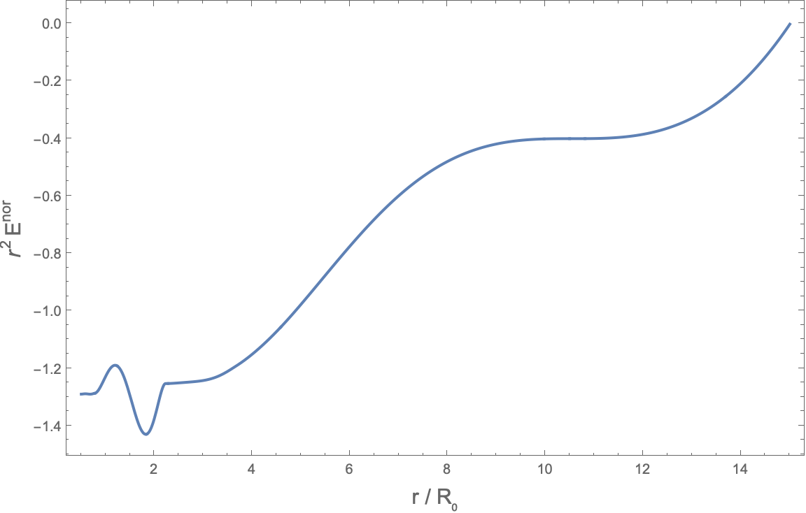
(a) a

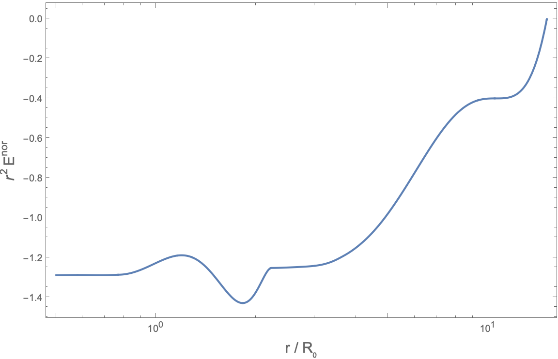
(b) b

Figure 3: Normalized fluctuation flux $r^{2}E_{\mathrm{fluc}}^{(\mathrm{nor})}(r)$ associated with the gauge-field zero mode. The left panel shows the profile on a linear radial scale, while the right panel uses a logarithmic scale to resolve the near-boundary region. The negative dip at small $r$ reflects suppression of the electric field by the scalar cloud in the near-horizon (IR) region. The apparent zero of the flux at $r=r_{\mathrm{IR}}$ is a boundary artifact resulting from the imposed condition $a_{t}^{\prime}(r_{\mathrm{IR}})=0$ and must not be interpreted as full screening. Physical screening is instead determined by the integrated cloud charge $q_{\mathrm{eff}}$, which remains finite, implying partial screening of the background BTZ electric field.

7 Discussion and Outlook

The results presented in this work can be viewed as the electric analogue of the magnetic hairy black holes studied in seminal works by Gubser and by Maldacena and collaborators. In particular, the appearance of a scalar condensate sourced by a background gauge field closely parallels the mechanism underlying magnetic instabilities and W–boson condensation in asymptotically AdS spacetimes gubser2005phase; maldacena2021comments; Aharony:2023amq. In those constructions, a background magnetic field drives the effective mass of charged modes below the Breitenlohner–Freedman bound, triggering an instability that is resolved by the formation of a static, spatially extended condensate. The resulting configuration corresponds to a genuine hairy black hole and provides a nonlinear completion of the original instability. In this sense, the present work realizes a closely related mechanism, but for an electric background field rather than a magnetic one.
The key novelty of our analysis is that we explicitly construct and analyze the backreacted electric screening cloud in the near-horizon region of an extremal charged BTZ black hole. While the existence of an electric instability in AdS₂ backgrounds has been known since early work on charged scalars and the BF bound Gubser:2002vv, the fully developed endpoint of this instability has not been previously analyzed in a controlled gravitational setting. Here we show that the instability is resolved by a static scalar condensate that partially screens the electric field and modifies the near-horizon geometry in a self-consistent manner.
A crucial feature of the construction is the extremality of the background. Only in the extremal limit does the near-horizon geometry develop an exact $\mathrm{AdS}_{2}$ throat with a constant electric field, allowing the instability to persist indefinitely and form a stationary cloud. The resulting configuration should therefore be viewed as an extremal analogue of magnetic hairy black holes, rather than as a generic feature of non-extremal geometries. Indeed, away from extremality the throat is cut off at finite temperature, and the instability is expected to become dynamical rather than static.
From this perspective, our results suggest that extremal charged black holes admit a richer set of infrared phases than previously appreciated. The screening cloud we construct represents a genuine new branch of solutions in which electric flux is partially absorbed by charged matter rather than being supported solely by the classical gauge field. This mechanism is closely analogous to the magnetic screening discussed in maldacena2021comments, but differs in both physical interpretation and technical implementation due to the distinct role of electric fields in AdS₂.
It is natural to ask whether the screening phenomenon described in this work admits an interpretation directly in the dual two–dimensional conformal field theory. In a CFT₂ with a conserved $U(1)$ current, modular invariance strongly constrains the structure of charged states and implies that the spectrum organizes in terms of the effective combination $\Delta_{\rm eff}=\Delta-\frac{Q^{2}}{2k}$, where $k$ is the current algebra level. This structure underlies the universal form of the charged Cardy regime and plays a central role in recent bootstrap analyses of large-$c$ CFTs with global symmetries Hartman:2014oaa; Benjamin:2016fhe; Kraus:2018pax. In this light, the appearance of a screening cloud in the near-horizon region of an extremal charged BTZ black hole admits a natural qualitative interpretation. If the CFT₂ contains sufficiently light charged operators—i.e. operators with small $\Delta_{\rm eff}$—then the extremal sector is not isolated but can reorganize through the participation of charged degrees of freedom. From the bulk perspective, this manifests as an instability of the naive AdS₂ throat and the formation of a charged condensate that screens the background electric field.
We emphasize that we do not claim a sharp equivalence between the existence of light charged operators and the appearance of a screening cloud, nor do we attempt a bootstrap derivation of this phenomenon. Rather, our results suggest a consistent physical picture in which the infrared structure of extremal charged black holes is sensitive to the charged operator content of the dual CFT. Establishing a precise quantitative relation between the spectrum of light charged operators and the onset of bulk screening would be an interesting direction for future work.
Finally, the analysis naturally suggests several extensions. Most importantly, it would be interesting to generalize the construction to near-extremal geometries, where the AdS₂ throat acquires a finite temperature. In that case, one expects the static cloud to evolve into a long-lived but dynamical configuration, with potential implications for thermalization and late-time dynamics. It would also be interesting to explore whether similar electric screening mechanisms arise in higher-dimensional charged black holes, where related instabilities have been observed but not yet fully understood. We leave these directions for future work.

Appendix A Variation of action

A.1 Variation of the bulk action

Variation of the bulk term is given by:

$$\delta S_{\rm bulk}=\frac{1}{2}\int_{r=r_{0}}dt\left[\Phi^{*}\partial_{r}\delta\Phi+(\partial\Phi)^{*}\delta\Phi\right]$$ (118)

where $\Phi(r)$ and $\partial_{r}\Phi(r)$ are given by:

$$\Phi(r) \simeq A_{-}r^{\Delta_{-}}+A_{+}r^{\Delta_{+}}$$ (119)

$$\partial_{r}\Phi \simeq\Delta_{-}A_{-}r^{\Delta_{-}-1}+\Delta_{+}A_{+}r^{\Delta_{+}-1}$$ (120)

and the variation of the two above equations is given by:

$$\delta\Phi \simeq\delta A_{-}r^{\Delta_{-}}+\delta A_{+}r^{\Delta_{+}}$$ (121)

$$\partial(\delta\Phi) \simeq\Delta_{-}\delta A_{-}r^{\Delta_{-}-1}+\Delta_{+}\delta A_{+}r^{\Delta_{+}-1}.$$ (122)

Expading the first term of (118), we have

$$\Phi^{*}\partial_{r}\delta\Phi\simeq\left(A_{-}^{*}r^{\Delta_{-}}+A_{+}^{*}r^{\Delta_{+}}\right)\left(\Delta_{-}\delta A_{-}r^{\Delta_{-}-1}+\Delta_{+}\delta A_{+}r^{\Delta_{+}-1}\right),$$ (123)

which gives four terms, but what matters to us is the leading term

$$\Phi^{*}\partial_{r}\delta\Phi\supset A_{-}^{*}\Delta_{-}\delta A_{-}r^{2\Delta-1}.$$ (124)

Using $\Delta_{-}=1/2-\mu$, we see that $2\Delta_{-}-1=-2\mu$, therfore for first term in (118) variation we can write:

$$\Phi^{*}\partial_{r}\delta\Phi\supset\Delta_{-}r^{-2\mu}A_{-}^{*}\delta A_{-}.$$ (125)

Similaryl, for the second term we have:

$$\left(\partial_{r}\Phi\right)^{*}\delta\Phi\simeq\left(\Delta_{-}A_{-}^{*}r^{\Delta_{-}-1}+\dots\right)\left(\delta A_{-}r^{\Delta_{-}}+\dots\right),$$ (126)

and again, the relevant terms for us are

$$\left(\partial_{r}\Phi\right)^{*}\delta\Phi\supset\Delta_{-}r^{-2\mu}A_{-}^{*}\delta A_{-}.$$ (127)

Now we combine (125) and (127) and substitute them into (118) at the UV cutoff $r=r_{0}$ to obtain the following:

$$\delta S_{\rm bulk}=\frac{1}{2}\int dt\left[\Delta_{-}r_{0}^{-2\mu}+\Delta_{-}r_{0}^{-2\mu}\right]A_{-}^{*}\delta A_{-}+\text{c.c}.$$ (128)

Finally, using $\Delta_{-}=1/2-\mu$, we obtain equation:

$$\delta S_{\rm bulk}=\int dt\left[\frac{1-2\mu}{2}r_{0}^{-2\mu}A_{-}^{*}\delta A_{-}\right]+\text{c.c}.$$ (129)

A.2 Variation of the first boundary term

We now add a local boundary term at the cutoff $r=r_{0}$,

$$S_{\rm bdy}^{(1)}=-\frac{1-2\mu}{2}\int_{r=r_{0}}dt\sqrt{-\hat{g}}\mid\Phi\mid^{2}.$$ (130)

Near the boundary $\mid\Phi\mid^{2}$ is now given by:

$$\mid\Phi\mid^{2}\simeq\mid A_{-}\mid^{2}r^{-2\Delta_{-}}+\left(A_{-}^{*}A_{+}+A_{+}^{*}A_{-}\right)r^{\Delta_{-}+\Delta_{+}}+\mid A_{+}\mid^{2}r^{-2\Delta_{+}}$$ (131)

where the leading term now is given by:

$$\mid\Phi\mid^{2}\supset\mid A_{-}\mid^{2}r^{1-2\mu}+\dots$$ (132)

where $2\Delta_{-}=1-2\mu$ and the induced metric on $r=r_{0}$ gives us a factor of $\sqrt{\hat{g}}\propto r_{0}^{-1}$. Taking its variation we find the following:

$$\delta S_{\rm bdy}^{(1)}=-\frac{1-2\mu}{2}\int_{r=r_{0}}dt\sqrt{-\hat{g}}\left(\Phi^{*}\delta\Phi+\Phi\delta\Phi\right).$$ (133)

We can now write:

$$\begin{split}\delta S_{\rm bdy}^{(1)}=-\,\frac{1-2\mu}{2}\int d\omega\Big[C\,r_{0}^{-2\mu}(A_{-}^{*}\delta A_{-}+\text{c.c.})+C(A_{+}^{*}\delta A_{-}+A_{-}^{*}\delta A_{+}+\text{c.c.})\\ \qquad\qquad\qquad\qquad+\,C\,r_{0}^{2\mu}(A_{+}^{*}\delta A_{+}+\text{c.c.})\Big].\end{split}$$ (134)

A.3 Variation of the second term

We now perturb this $\rm DCFT_{1}$ by the relevant $\mid\Phi\mid^{2}$. In $\rm AdS$ language this is a double-trace deformation. Therefore, we add the following second boundary term

$$S_{\rm bdy}^{(2)}=-f_{0}\int_{r=r_{0}}dt\sqrt{-\hat{g}}r_{0}^{2\mu}\mid\Phi\mid^{2}.$$ (135)

Near the boundary our solution is given by (132), so

$$\mid\Phi\mid^{2}\supset\mid A_{-}\mid^{2}r^{1-2\mu}+\dots,$$ (136)

and from our induced metric, $\sqrt{-\hat{g}}\sim R_{A}/r$, we find that

$$\sqrt{-\hat{g}}\mid\Phi\mid^{2}\supset C\mid A_{-}\mid^{2}r^{-2\mu}.$$ (137)

Multiplying by $r_{0}^{2\mu}$ makes $\mid A_{-}\mid^{2}$ contribution finite at the cutoff:

$$\sqrt{-\hat{g}}r_{0}^{2\mu}\mid\Phi\mid^{2}\supset C\mid A_{-}\mid^{2}+\mathcal{O}\left(r_{0}^{2\mu}\right).$$ (138)

So, by adding the second boundary term, we are re-introducing an $A_{-}^{*}A_{-}$ term with a finite coefficient $f_{0}$, which will compete with the cross term from $S_{\rm bulk}+S_{\rm bdy}^{(1)}$.
At leading order in small $r_{0}$ the variation of the second boundary term is given by:

$$\delta S_{\rm bdy}^{(2)}\simeq-f_{0}C\int d\omega\left(A_{-}^{*}\delta A_{-}+A_{-}\delta A_{-}^{*}\right)+\mathcal{O}\left(r_{0}^{2\mu}\right).$$ (139)

After adding both boundary terms, the leading parts of the variation are:

• from $S_{\rm bulk}+S_{\rm bdy}^{(1)}$: the cross term

  $$\sim 2\mu\left(A_{+}^{*}\delta A_{-}+A_{-}^{*}\delta A_{+}\right)$$ (140)

  
  

• from $\delta S_{\rm bdy}^{(2)}$ we have

  $$\sim f_{0}\left(A_{-}^{*}\delta A_{-}+\text{c.c}\right)$$ (141)

So at leading order in small $r_{0}$ for the full variation we have

$$\delta\!\left(S_{\rm bulk}+S_{\rm bdy}^{(1)}+S_{\rm bdy}^{(2)}\right)\simeq\int d\omega\Big[2\mu\!\left(A_{+}^{*}\,\delta A_{-}+A_{-}^{*}\,\delta A_{+}\right)$$ (142)

$$\qquad\qquad\qquad\quad+\,f_{0}\!\left(A_{-}^{*}\,\delta A_{-}+A_{-}\,\delta A_{-}^{*}\right)\Big].$$

A.4 Derivation of Beta-function

We start with our boundary condition

$$\frac{A_{+}}{A_{-}}=R(r_{0},f)=-\frac{f}{r_{0}^{2\mu}\left[f-2\mu\right]}.$$ (143)

This ratio is a physical quantity and it depends on $r_{0}$, therefore we write

$$0=r_{0}\frac{d}{dr_{0}}R(r_{0},f(r_{0}))=\left(r_{0}\partial_{r_{0}}--\beta_{f}\partial_{f}\right)R(r_{0},f(r_{0}))$$ (144)

For fixed $f$ we find that

$$r_{0}\partial_{r_{0}}R(r_{0},f)=\frac{2\mu f}{f-2\mu}r_{0}^{-2\mu}.$$ (145)

Now holding $r_{0}$ fixed, varying $f$ we have:

$$R(r_{0},f)=-\frac{1}{r_{0}^{2\mu}}\frac{f}{f-2\mu}=-\frac{1}{r_{0}^{2\mu}}G(f),$$ (146)

where the derivative of $G(f)$ with respect to $f$ is given by

$$\partial_{f}G(f)=-\frac{2\mu}{\left(f-2\mu\right)^{2}}.$$ (147)

Then we can write

$$\partial_{f}R(r_{0},f)=\frac{2\mu}{r_{0}^{2\mu}\left(f-2\mu\right)^{2}}$$ (148)

Finally for (144) we have

$$0 =r_{0}\partial_{r_{0}}R-\beta_{f}\partial_{f}R$$ (149)

$$=\frac{2\mu f}{f-2\mu}-\beta_{f}\frac{2\mu}{r_{0}^{2\mu}\left(f-2\mu\right)^{2}}$$ (150)

$$=\frac{2\mu}{r_{0}^{2\mu}\left(f-2\mu\right)^{2}}\left[f(f-2\mu)-\beta_{f}\right],$$ (151)

from which we get our beta-function

$$\beta_{f}=-2\mu f+f^{2}.$$ (152)

Appendix B Boundary Two-Point Function and Double-Trace Flow in the AdS₂ Throat

In this section we compute the Euclidean propagator for the boundary mode dual to the radial solution of the charged scalar field in the near-horizon $\mathrm{AdS}_{2}$ region of the near-extremal charged BTZ black hole. We work entirely with the Whittaker solution obtained in the main text, imposing IR infalling boundary conditions and extracting the near-boundary coefficients $A_{\pm}(\omega)$. These coefficients determine the Euclidean Green’s function $G^{(0)}(\omega)$ at the alternate quantization fixed point. We then add a double-trace boundary deformation and obtain the exact resummed propagator.

B.1 Bulk Setup and Near-Boundary Expansion

In the $\mathrm{AdS}_{2}$ throat we use the Poincaré metric

$$ds^{2}=\frac{dr^{2}+dt_{E}^{2}}{r^{2}},$$ (153)

with $r\to 0$ the conformal boundary and $r\to\infty$ the horizon. The charged scalar $\Phi$ satisfies the Euclidean equation

$$\left(-\nabla^{2}+m_{\rm eff}^{2}+q^{2}A_{\mu}A^{\mu}\right)\Phi=0,$$ (154)

where the near-horizon gauge field is (Euclidean continuation)

$$A_{t_{E}}(r)=-\,\frac{iqE\ell^{2}}{r}.$$ (155)

We define the Whittaker parameters

$$\kappa=-i\,\frac{\ell^{2}qE}{\sqrt{2}},\qquad k=i\sqrt{2}\,\ell^{2}\omega,$$ (156)

and the effective $\mathrm{AdS}_{2}$ scaling exponent

$$\mu^{2}=\frac{1}{4}+m_{\rm eff}^{2}\ell^{2}-\frac{\ell^{4}q^{2}E^{2}}{4}.$$ (157)

The BF bound is violated when $\mu^{2}<0$.

B.2 IR Infalling Boundary Condition

The general radial solution in $x$-coordinates is

$$R(x)=C_{1}\,M_{\kappa,\mu}\!\left(\frac{k}{x}\right)+C_{2}\,W_{\kappa,\mu}\!\left(\frac{k}{x}\right).$$ (158)

Near the horizon ($x\to 0$, equivalently $r\to\infty$), the Whittaker functions behave as

$$W_{\kappa,\mu}\!\left(\frac{k}{x}\right)\sim\exp\!\left(-\frac{k}{2x}\right)\left(\frac{k}{x}\right)^{\kappa},$$ (159)

$$M_{\kappa,\mu}\!\left(\frac{k}{x}\right)\sim\frac{\Gamma(1+2\mu)}{\Gamma(\frac{1}{2}+\mu-\kappa)}\exp\!\left(+\frac{k}{2x}\right)\!\left(\frac{k}{x}\right)^{-\kappa}+\cdots.$$ (160)

For $k=i\sqrt{2}\,\ell^{2}\omega$, the phases $\exp(\pm k/2x)$ are oscillatory. The infalling condition selects the mode proportional to $\exp(-ik/2x)$, hence

$$R_{\rm IR}(x)\propto W_{\kappa,\mu}\!\left(\frac{k}{x}\right).$$ (161)

Thus we set $C_{1}=0$ and keep only the $W$-branch.

B.3 UV Asymptotics and Extraction of $A_{\text{\textpm}}$

At small argument $z\to 0$, the Whittaker function expands as

$$\begin{split}W_{\kappa,\mu}(z)=\frac{\Gamma(2\mu)}{\Gamma\!\left(\frac{1}{2}+\mu-\kappa\right)}z^{\frac{1}{2}-\mu}+\frac{\Gamma(-2\mu)}{\Gamma\!\left(\frac{1}{2}-\mu-\kappa\right)}z^{\frac{1}{2}+\mu}+\cdots.\end{split}$$ (162)

Setting $z=k/x$ and using $r=1/x$ gives the near-boundary form

$$R(r)=A_{-}(\omega)\,r^{\Delta_{-}}+A_{+}(\omega)\,r^{\Delta_{+}},\qquad\Delta_{\pm}=\frac{1}{2}\pm\mu,$$ (163)

with coefficients

$$A_{-}(\omega) =C_{2}\,k^{\frac{1}{2}-\mu}\,\frac{\Gamma(2\mu)}{\Gamma\!\left(\frac{1}{2}+\mu-\kappa\right)},$$ (164)

$$A_{+}(\omega) =C_{2}\,k^{\frac{1}{2}+\mu}\,\frac{\Gamma(-2\mu)}{\Gamma\!\left(\frac{1}{2}-\mu-\kappa\right)}.$$

The normalization constant $C_{2}$ cancels in the ratio:

$$\frac{A_{-}(\omega)}{A_{+}(\omega)}=k^{-2\mu}\,\frac{\Gamma(2\mu)}{\Gamma(-2\mu)}\,\frac{\Gamma\!\left(\frac{1}{2}-\mu-\kappa\right)}{\Gamma\!\left(\frac{1}{2}+\mu-\kappa\right)}.$$ (165)

B.4 Boundary Generating Functional

The Euclidean on-shell action from the bulk plus counterterm $S_{\rm bdy}^{(1)}$ reduces to

$$S_{\rm on-shell}=\int d\omega\,\left[A_{+}^{*}(\omega)\,A_{-}(\omega)+A_{-}^{*}(\omega)\,A_{+}(\omega)\right],$$ (166)

once we impose the alternate quantization condition $A_{+}=J(\omega)$, where $J(\omega)$ is the boundary source.
Varying with respect to $J$ gives the one-point function $\langle A_{-}(\omega)\rangle$, and the connected two-point function satisfies

$$\langle A_{-}(\omega)A_{-}^{*}(\omega^{\prime})\rangle=2\pi\delta(\omega-\omega^{\prime})\,G^{(0)}(\omega),$$ (167)

with

$$G^{(0)}(\omega)=-\,\left[\frac{A_{-}(\omega)}{A_{+}(\omega)}+\frac{A_{-}^{*}(\omega)}{A_{+}^{*}(\omega)}\right].$$ (168)

Using (165), one obtains the explicit form

$$G^{(0)}(\omega)=k^{-2\mu}\frac{4\,\Gamma(2\mu)}{\Gamma(1-2\mu)}\frac{\Gamma\!\left(\frac{1}{2}-\mu-\kappa\right)}{\Gamma\!\left(\frac{1}{2}+\mu-\kappa\right)}.$$ (169)

This is the analogue of eq. (A.13) in Aharony:2023amq; faulkner2011emergent; iqbal2010quantum; Iqbal:2011aj.