Fast Approximation Algorithm for Non-Monotone DR-submodular Maximization under Size Constraint

Abstract

This work studies the non-monotone DR-submodular Maximization over a ground set of $n$ subject to a size constraint $k$. We propose two approximation algorithms for solving this problem named FastDrSub and FastDrSub+. FastDrSub offers an approximation ratio of $0.044$ with query complexity of $O(n\log(k))$. The second one, FastDrSub+  improves upon it with a ratio of $1/4-\epsilon$ within query complexity of $(n\log k)$ for an input parameter $\epsilon>0$. Therefore, our proposed algorithms are the first constant-ratio approximation algorithms for the problem with the low complexity of $O(n\log(k))$. Additionally, both algorithms are experimentally evaluated and compared against existing state-of-the-art methods, demonstrating their effectiveness in solving the Revenue Maximization problem with DR-submodular objective function. The experimental results show that our proposed algorithms significantly outperform existing approaches in terms of both query complexity and solution quality.

1 Introduction

Submodular optimization problems have emerged in a wide range of applications, particularly in machine learning bach2013learning ; Das ; prajapat2024submodular , data mining ap-recommend ; ap-datasum , and combinatorial optimization vondrak08_welfare ; canh-joco19 ; tap-17 . Numerous applications related to influence propagation in social networks tap-17 ; vic-icml-2019 ; canh-joco19 ; canh_optlet ; canh_csonet19 ; canh-csonet18 , budget allocation soma-nips-15 , recommendation systems recomend-icml , data summarization sc-dis-alg-nips15 , and active set selection Norouzi_NIPS2016 can all be framed as Submodular Maximization problems. A set function $f:2^{E}\mapsto\mathbb{R}_{+}$, defined on all subsets of a ground set $E$ size $n$, is submodular iff it satisfies the diminishing return property, i.e., for $X\subseteq Y\subseteq E$, and an element $e\notin Y$, we have:

$$f(X\cup\{e\})-f(X)\geq f(Y\cup\{e\})-f(Y).$$

The Submodular Maximization problem has been studied under various constraints, including unconstrained feige2011maximizing , size constraint nemhauser1978analysis , knapsack constraint  sviridenko2004note , matroid constraint calinescu2007maximizing , etc. Nevertheless, the traditional submodular set function falls short in addressing specific real-world scenarios that permit multiple instances of an element from the ground set to be selected. To address this limitation, Soma and Yoshida  soma-nips-15 proposed an extension of the function $f$ to the integer lattice $\mathbb{Z}^{E}_{+}$, introducing a generalized form of submodularity in this context, termed diminishing return submodular (DR-submodular). For a vector $\textbf{x}\in\mathbb{Z}^{E}_{+}$, denote by $\textbf{x}(e)$ the value of x’s coordinate corresponding to an element $e$. For $\textbf{x},\textbf{y}\in\mathbb{Z}_{+}^{E}$, we say that $\textbf{x}\leq\textbf{y}$ iff $\textbf{x}(e)\leq\textbf{y}(e),\forall e\in E$. The function $f:\mathbb{Z}^{E}_{+}\mapsto\mathbb{R}_{+}$ is diminishing return submodular (DR-submodular) on integer lattice if:

$$f(\textbf{x}+\delta{\mathbf{1}}_{e})-f(\textbf{x})\geq f(\textbf{y}+\delta{\mathbf{1}}_{e})-f(\textbf{y})$$

for $\textbf{x},\textbf{y}\in\mathbb{Z}^{E}_{+},\textbf{x}\leq\textbf{y}$. In this work, we consider the DR-submodular Maximization under Size constraint ($\mathsf{DrSMC}$) problem, defined as follows:

Definition 1($\mathsf{DrSMC}$ problem).

Given a DR-submodular function $f:\mathbb{Z}^{E}_{+}\mapsto\mathbb{R}_{+}$, a bounded lattice B, and a positive integer $k>0$. The problem asks to find $\textbf{x}\leq\textbf{B}$ with the total size $\|\textbf{x}\|_{1}\leq k$ such that $f(\textbf{x})$ is maximized, i.e,

$$\max_{\textbf{x}\in\mathbb{Z}^{E}_{+}}\ \ \ f(\textbf{x})\ \ \mbox{subject to:}\ \ \|\textbf{x}\|_{1}\leq k,\textbf{0}\leq\textbf{x}\leq\textbf{B}$$ (1)

where $\textbf{B}=B\cdot{\mathbf{1}}$ and $\|\textbf{x}\|_{1}=\sum_{e\in E}\textbf{x}(e)$. Without loss of generality, we set $\textbf{B}=k\cdot{\mathbf{1}}$. The integer lattice can be represented as a multiset of size $O(nk)$, allowing the direct adaptation of existing algorithms for the Submodular Maximization under a size constraint ($\mathsf{DrSMC}$) problem. However, the fastest known algorithm for $\mathsf{DrSMC}$, proposed by buchbinder2014submodular , requires $\Omega(nk)$ oracle queries to evaluate the function $f$, which is not polynomial in the size of the input. Importantly, since $k$ is an integer and can be encoded using only $O(\log k)$ bits, any algorithm with complexity $O(\mathrm{poly}(k))$ is not necessarily polynomial in the input size. In this setting, we assume access to a value oracle that returns $f(\textbf{x})$ when queried with a multiset x.

Recently, Ene and Nguyen ene2016reduction proposed a reduction technique that transforms the problem of optimizing DR-submodular functions into a standard submodular maximization problem, thereby enabling the application of well-established results in submodular optimization. Specifically, the $\mathsf{DrSMC}$ problem, after applying the reduction ene2016reduction , can be transformed into the following submodular maximization problem under a knapsack constraint:

$$\max_{S\subseteq E^{\prime}}\quad g(S)\quad\text{subject to:}\quad c(S)\leq k,$$ (2)

where $E^{\prime}=\bigcup_{e\in E}\{(e,j):j\in[t_{e}]\}$ is the new ground set obtained by decomposing each integer variable $\textbf{x}(e)$ into a sum of smaller weights $a_{e,j}\leq\varepsilon k$. Each $a_{e,j}$ represents a small positive integer weight used to decompose the integer variable $\textbf{x}(e)$ into a sum of binary variables, ensuring that any value in the range $[0,B_{e}]$ can be expressed as a subset sum of $\{a_{e,j}\}_{j=1}^{t_{e}}$. The submodular function $g(S)$ is defined as $g(S):=f(\textbf{x})$, where $\textbf{x}(e)=\sum_{j:(e,j)\in S}a_{e,j}$ for all $e\in E$, and the cost function is $c(S):=\sum_{(e,j)\in S}a_{e,j}$. As a result of the reduction, the size of the new search space becomes $O(n\log k)$ instead of $O(n)$ as in the original DR-submodular problem. One can apply the best-known approximation ratio, together with efficient practical algorithms for the submodular knapsack problem, as established in pham-ijcai23 ; Han2021_knap , to obtain a ratio of $1/4-\epsilon$. However, a weakness randomized algorithms is that they only keep the ratio in expectation and the experimental results for real-world dataset may be unstable. In contrast, recent studies have demonstrated that deterministic algorithms often yield superior empirical performance, primarily due to their stability across diverse datasets kuhnle2021bquick ; kdd-ChenK23 ; han-neurips20 ; li-linear-knap-nip22 . Moreover, as data scales to massive sizes, it becomes increasingly important to design approximation algorithms for $\mathsf{DRSC}$ that minimize oracle queries to ensure computational efficiency.

These observations raise two important research questions: (1) Can we design new algorithms that achieve a comparable approximation ratio while improving the oracle query complexity, thereby enhancing the practical efficiency of the reduction framework? (2) Is it possible to develop a deterministic algorithm for the DR-submodular maximization problem under a size constraint with an approximation guarantee comparable to the current randomized methods? Addressing these questions would not only improve the computational performance of DR-submodular optimization on large-scale instances but also advance the theoretical understanding of submodular maximization over the integer lattice.

Our Contributions and Techniques.

In this work, we try to address the above two questions. Our main contributions are as follows:

• We propose two algorithms: FastDrSub achieves an approximation ratio of $0.044$ with a query complexity of $O(n\log(k))$, and FastDrSub+ achieves an approximation ratio of $\frac{1}{4}-\epsilon$ with a query complexity of $O\left(\frac{n}{\epsilon}\log\left(\frac{k}{\epsilon}\right)\right)$ for the $\mathsf{DrSMC}$ problem. Although the best-known theoretical approximation ratio is $0.401$ buchbinder2024constrained , the corresponding algorithm has polynomial complexity and is therefore impractical. Compared with the fastest near-linear algorithms pham-ijcai23 ; Han2021_knap , which rely on randomness, our approach achieves a similar complexity but remains deterministic. To the best of our knowledge, this is the first deterministic algorithm that achieves the strongest known approximation ratio in the near-linear time setting (for details, see Table 1).

• We perform comprehensive experiments on Revenue Maximization benchmarks, demonstrating that our algorithms attain solution quality comparable to the current state of the art while requiring fewer oracle queries.

Table 1: We compare several algorithms for the maximization of a non-monotone DR-submodular function under a size constraint. Each algorithm is evaluated by its approximation guarantee and the number of oracle queries required. Let $\epsilon>0$ denote the accuracy parameter, $k$ the size budget, and $\|\mathbf{b}\|_{\infty}=k$ the maximum coordinate bound. In particular, the oracle complexities of RLA and SMKRANACC have been rederived using the reduction framework of Ene and Nguyen ene2016reduction , which increases the ground‐set size to $n(2\log k+1)$. Note that the rederived complexities are stated with respect to this enlarged ground set, but they do not explicitly account for the additional computational overhead introduced by the reduction itself.

Reference	Approx. Factor	Query complexity	Type
RLA pham-ijcai23 +Reductionene2016reduction	$\frac{1}{4}-\epsilon$	$O\left(\frac{n}{\epsilon}\log(k)\log(\frac{1}{\epsilon})\right)$	Randomized
SMKRANACCHan2021_knap +Reductionene2016reduction	$\frac{1}{4}-\epsilon$	$O\left(\frac{n}{\epsilon}\log(k)\log(\frac{k}{\epsilon})\right)$	Randomized
FastDrSub (this paper)	$\displaystyle 0.044$	$O(n\log k)$	Deterministic
FastDrSub+ (this paper)	$\tfrac{1}{4}-\epsilon$	$O(\frac{n}{\epsilon}\log(\frac{1}{\epsilon})\log(k))$	Deterministic

To attain constant-factor approximation guarantees within $O(n\log k)$ query complexity, we introduce a novel combinatorial algorithmic framework comprising two key phases: (1) In the first phase, we partition the solution space into two subspaces—one consisting of elements whose cardinality does not exceed $\alpha k$ for $\alpha\in(0,1)$, and the other containing the remaining elements. We then compute near-optimal solutions independently within each subspace and strategically merge them to obtain a unified solution that achieves a constant approximation ratio of $0.044$ ( FastDrSub Algorithm ). (2) In the second phase, we enhance the approximation ratio to nearly $1/4$ via the FastDrSub+ algorithm. This improvement leverages the output of FastDrSub and employs a carefully designed greedy thresholding technique to sequentially construct two candidate solutions. The construction is guided by the structural properties of two auxiliary vectors, x and y, which satisfy the condition $\min\{\textbf{x}(e),\textbf{y}(e)\}=0$ for all $e\in V$, as formalized in Lemma 1.

Organization

This paper is organized as follows: The Related Works section 2 presents previous research and existing methods. The Preliminaries section 3 provides the basic concepts and theoretical foundations necessary for understanding the proposed algorithms. The Proposed Algorithm section 4 describes the details of the proposed algorithm, including the steps and underlying theory. The Experimental Evaluation section  5 presents the experimental results and analysis of the algorithm’s performance. Finally, the Conclusion section  6 summarizes the key findings and outlines directions for future research.

2 Related Works

In this section, we review the literature on optimization algorithms for $\mathsf{DRSC}$.

Monotone DR-submodular functions.

Soma and Yoshida soma-nips-15 were the first to extend the notion of submodular functions to the integer lattice by introducing the concept of DR-submodularity and proposing a bicriteria approximation algorithm that simultaneously accounts for both the objective and cost functions. Subsequently, in a follow-up work soma2018maximizing , the authors developed two deterministic algorithms that achieve a $1-\frac{1}{e}-\epsilon$ approximation for maximizing monotone DR-submodular and general lattice submodular functions, with time complexities of $O\left(\frac{n}{\epsilon}\log k\log\frac{k}{\epsilon}\right)$ and $O\left(\frac{n}{\epsilon^{2}}\log k\log\frac{k}{\epsilon}\log\tau\right)$, respectively, where $k$ denotes the size budget and the maximum coordinate bound, and $\tau$ denotes both the ratio between the maximum function value and the minimum positive marginal gain. Lai et al. (2019) lai2019monotone introduced a randomized algorithm, though it suffers from instability in the number of oracle calls. More recently, Schiabel et al. (2025) schiabel2021randomized proposed the Stochastic Greedy Lattice (SGL) algorithm, which extends the stochastic greedy sampling strategy to monotone DR-submodular functions over integer lattices. SGL achieves an approximation guarantee of $\left(1-\frac{1}{e}-\hat{t}\epsilon\right)$ with probability greater than $\frac{1}{2}$, where $\hat{t}$ is a small constant dependent on the number of iterations.

Non-monotone DR-submodular functions.

Designing algorithms for non-monotone DR-submodular functions is significantly more challenging than for the monotone case due to the potential decrease in function values. Gottschalk and Peis (2015) gottschalk2015submodular proposed a Double Greedy algorithm for maximizing submodular functions over bounded integer lattices, achieving a $\frac{1}{3}$ approximation ratio, albeit with pseudopolynomial complexity. Ene et al. (2020) ene2020parallel developed a parallel algorithm for non-monotone DR-submodular maximization but restricted it to the continuous domain. Li et al. (2023) li2023dr further improved algorithmic efficiency using an adaptive step size approach.

As mentioned in the introduction, by applying the reduction technique proposed by Ene and Nguyenene2016reduction , the $\mathsf{DrSMC}$ can be transformed into a standard submodular maximization problem under a knapsack constraint ($\mathsf{SMK}$). In the following, we review the line of research focused on the $\mathsf{SMK}$ problem. The first work to address the $\mathsf{SMK}$ problem in the non-monotone case was proposed by Lee_nonmono_matroid_knap , achieving an approximation ratio of $5+\epsilon$ with polynomial query complexity. Subsequently, many follow-up studies have aimed to improve algorithmic efficiency BuchbinderF19-bestfactor ; Gupta_nonmono_constrained_submax ; fast_icml ; nearly-liner-der-2018 ; best-dla ; pham-ijcai23 ; Han2021_knap . Among these, the method in BuchbinderF19-bestfactor achieved the best approximation factor of $2.6$, though at the cost of high oracle complexity. Conversely, the algorithm in pham-ijcai23 attained the lowest query complexity—linear in the input size—while achieving an approximation ratio of $4+\epsilon$.

To the best of our knowledge, no existing work has directly addressed the problem of maximizing non-monotone DR-submodular functions under size constraints. In this paper, we propose a novel approach to address this problem.

3 Preliminaries

For a positive integer $k\in\mathbb{N}$, $[k]$ denotes the set $\{1,\ldots,k\}$. Given a ground set $E=\{e_{1},\ldots,e_{n}\}$, we denote $\textbf{x}(e)$ as the value of x’s coordinate corresponding to an element $e$, define the $e$-th unit vector ${\mathbf{1}}_{e}$ with ${\mathbf{1}}_{e}(t)=1$ if $t=e$ and ${\mathbf{1}}_{e}(t)=0$ if $t\neq e$. For $\textbf{x},\textbf{y}\in\mathbb{Z}_{+}^{E}$, we say that $\textbf{x}\leq\textbf{y}$ iff $\textbf{x}(e)\leq\textbf{y}(e),\forall e\in E$. For $\textbf{x}=(x_{1},x_{2},\ldots,x_{n})$ and $\textbf{y}=(y_{1},y_{2},\ldots,y_{n})$, we define

$$\textbf{x}\wedge\textbf{y} =(\min\{x_{1},y_{1}\},\min\{x_{2},y_{2}\},\ldots,\min\{x_{n},y_{n}\})$$ (3)

$$\textbf{x}\vee\textbf{y} =(\max\{x_{1},y_{1}\},\max\{x_{2},y_{2}\},\ldots,\max\{x_{n},y_{n}\}).$$ (4)

For function $f:\mathbb{Z}_{+}^{E}\mapsto\mathbb{R}_{+}$, we define $f(\textbf{x}|\textbf{y})=f(\textbf{x}+\textbf{y})-f(\textbf{y})$. For $\textbf{x}\in\mathbb{Z}^{E}_{+}$, we denote by $\{\textbf{x}\}$ the set of elements appears in x times and with a subset, i.e, $\{\textbf{x}\}=\{e\in E,\textbf{x}(e)\geq 1\}$ and the size of x as $\|\textbf{x}\|_{1}=\sum_{e\in\{\textbf{x}\}}\textbf{x}(e)$. A function $f:\mathbb{Z}_{+}^{E}\mapsto\mathbb{R}$ is monotone if $f(\textbf{x})\leq f(\textbf{y}$) for all $\textbf{x},\textbf{y}\in\mathbb{Z}_{+}^{E}$ with $\textbf{x}\leq\textbf{y}$. The function $f$ is lattice submodular iff

$$f(\textbf{x})+f(\textbf{y})\geq f(\textbf{x}\vee\textbf{y})+f(\textbf{x}\wedge\textbf{y})$$ (5)

for any $\textbf{x},\textbf{y}\in\mathbb{Z}_{+}^{E}$. The function $f$ is said to be DR-submodular iff

$$f(\textbf{x}+{\mathbf{1}}_{e})-f(\textbf{x})\geq f(\textbf{y}+{\mathbf{1}}_{e})-f(\textbf{y})$$ (6)

for all $\textbf{x}\leq\textbf{y}$, $e\in E$. If $f$ is DR-submodular then one implies $f$ is lattice submodular soma-nips-15 . We assume that we can access $f$ through an oracle, i.e., for any vector $\textbf{x}\in\mathbb{Z}_{+}^{E}$, it returns the value of $f(\textbf{x})$.

The following basic lemmas are established as foundational tools for our theoretical analysis.

Lemma 1.

For any $\textbf{s}\in\mathbb{Z}^{E}_{+}$ and two vectors $\textbf{x},\textbf{y}\in\mathbb{Z}^{E}_{+}$ such that $\textbf{x}\wedge\textbf{y}=\textbf{0}$ we have

$$f(\textbf{s})\leq f(\textbf{s}\vee\textbf{x})+f(\textbf{s}\vee\textbf{y}).$$ (7)

Proof.

Since $f$ is a non-negative and lattice submodular function, we have

$$f(\textbf{s}\vee\textbf{x})+f(\textbf{s}\vee\textbf{y}) \geq f(\textbf{s}\vee\textbf{x}\vee\textbf{y})+f((\textbf{s}\vee\textbf{x})\wedge(\textbf{s}\vee\textbf{y}))$$ (8)

$$=f(\textbf{s}\vee\textbf{x}\vee\textbf{y})+f(\textbf{s})$$ (9)

$$\geq f(\textbf{s})$$ (10)

where the inequality (8) is due to the lattice submodular, the inequality (9) is due to $\textbf{x}\wedge\textbf{y}=\textbf{0}$, the inequality (10) is due to the non-negative of $f$. The proof is competed. ∎

Lemma 2.

For any $\textbf{x}\in\mathbb{Z}^{E}_{+}$ and an integer number $t\geq 0$, then $f(t{\mathbf{1}}_{e}|\textbf{x})\leq tf({\mathbf{1}}_{e}|\textbf{x})$.

Proof.

By the Dr-submodularity of $f$, we have

$$f(t{\mathbf{1}}_{e}\mid\textbf{x}) =f(\textbf{x}+t{\mathbf{1}}_{e})-f(\textbf{x})$$

$$=f({\mathbf{1}}_{e}\mid\textbf{x}+(t-1){\mathbf{1}}_{e})+f({\mathbf{1}}_{e}\mid\textbf{x}+(t-2){\mathbf{1}}_{e})+\ldots+f({\mathbf{1}}_{e}\mid\textbf{x})$$

$$\leq tf({\mathbf{1}}_{e}\mid\textbf{x})$$

which completes the proof. ∎

4 The Proposed Algorithms

In this section, we present two algorithms: Fast Approximation (FastDrSub) and Fast Approximation Plus (FastDrSub+) for $\mathsf{DrSMC}$ problem. FastDrSub retains an approximation ratio of $0.044$ (Theorem 4.1) and takes the query complexity of $O(n\log k)$. FastDrSub+ built upon FastDrSub, enhances the optimization process by employing the constant number guess of optimal solutions with greedy threshold badanidiyuru2014fast and therefore improve the approximation ratio to nearly $\frac{1}{4}$ (Theorem 4.2) without increasing the query complexity of $O(n\log k)$.

4.1 Fast Approximation Algorithm (FastDrSub)

The FastDrSub algorithm takes as input a DR-submodular function $f$, a finite ground set $E$ of size $n$, a size budget $k\in\mathbb{Z}_{>0}$, and a threshold parameter $\alpha\in(0,1)$. Its goal is to output a solution vector $\textbf{z}\in\mathbb{Z}_{\geq 0}^{E}$ satisfying $\|\mathbf{z}\|_{1}\leq k$, which approximately maximizes $f(\textbf{z})$. The core idea of the algorithm is to simultaneously construct two disjoint solution vectors, x and y, using a dynamic-threshold rule, thus facilitating a clear theoretical analysis based on Lemma 1.

Specifically, it first performs a binary search over $d\in(\alpha k,k]$ to identify the pair $(d_{\max},e_{\max})$ that maximizes $f(d\mathbf{1}_{e})$, retaining this singleton choice as an independent candidate (Line 1). Next, starting from $\textbf{x}=\textbf{y}=\mathbf{0}$, the algorithm iterates through each element $e\in E$. For each element, it identifies the largest integer $d\leq\alpha k$ whose marginal gain satisfies $f(\mathbf{1}_{e}\mid\textbf{x}+(d-1)\mathbf{1}_{e})\geq\frac{f(\textbf{x})}{k}$ (and analogously for y), then updates only the vector exhibiting the larger marginal gain.

Consequently, the two vectors evolve along distinct trajectories, guided by the same value-dependent threshold. After processing all elements, the algorithm trims the most recently added units from each vector, obtaining vectors $\textbf{x}^{\prime}$ and $\textbf{y}^{\prime}$ with $\|\textbf{x}^{\prime}\|_{1}\leq k$ and $\|\textbf{y}^{\prime}\|_{1}\leq k$. Finally, the best solution among $\textbf{x}^{\prime}$, $\textbf{y}^{\prime}$, and $d_{\max}\mathbf{1}_{e_{\max}}$ is returned. The overall procedure requires only $O(n\log k)$ oracle calls and guarantees a proven constant-factor approximation ratio.

Input: $f:\mathbb{Z}^{E}_{+}\mapsto\mathbb{R}_{+}$,$E$, $k$, $\alpha$

1 $(d_{max},e_{max})\leftarrow\arg\max_{e\in E,\ d\in\mathbb{Z},\ \alpha k<d\leq k}\ f(d{\mathbf{1}}_{e})$ by using the binary search

2$\textbf{x}\leftarrow\textbf{0}$, $\textbf{y}\leftarrow\textbf{0}$

3foreach $e\in E$ do

4  

5  $d_{(\textbf{x},e)}\leftarrow\max\{d\in\mathbb{Z}\mid 0<d\leq\alpha k,\ f({\mathbf{1}}_{e}\mid\textbf{x}+(d-1){\mathbf{1}}_{e})\geq\frac{f(\textbf{x})}{k}\}$ by using the binary search

6  $d_{(\textbf{y},e)}\leftarrow\max\{d\in\mathbb{Z}\mid 0<d\leq\alpha k,\ f({\mathbf{1}}_{e}\mid\textbf{y}+(d-1){\mathbf{1}}_{e})\geq\frac{f(\textbf{y})}{k}\}$ by using the binary search

7  if $f(d_{(\textbf{x},e)}{\mathbf{1}}_{e}\mid\textbf{x})\geq f(d_{(\textbf{y},e)}{\mathbf{1}}_{e}\mid\textbf{y})$ then

8     $\textbf{x}\leftarrow\textbf{x}+d_{(\textbf{x},e)}{\mathbf{1}}_{e}$

9     else

10       $\textbf{y}\leftarrow\textbf{y}+d_{(\textbf{y},e)}{\mathbf{1}}_{e}$

11       end if

12      

13       end foreach

14       Define $\{e_{1},e_{2},\ldots,e_{t}\}$ as the set of last $t$ elements added into x, i.e, $\textbf{x}_{t}=\sum_{i=1}^{t}\textbf{x}(e_{t}){\mathbf{1}}_{e_{t}}$

15       $\textbf{x}^{\prime}\leftarrow\arg\max_{\textbf{x}_{t}:|\textbf{x}_{t}|\leq k}t$

16       Define $\{e^{\prime}_{1},e^{\prime}_{2},\ldots,e^{\prime}_{t}\}$ as the set of last $t$ elements added into y, i.e, $\textbf{y}_{t}=\sum_{i=1}^{t}\textbf{y}(e^{\prime}_{t}){\mathbf{1}}_{e^{\prime}_{t}}$

17       $\textbf{y}^{\prime}\leftarrow\arg\max_{\textbf{y}_{t}:|\textbf{y}_{t}|\leq k}t$

18       $\textbf{z}\leftarrow\arg\max_{\textbf{z}^{\prime}\in\{\textbf{x}^{\prime},\textbf{y}^{\prime},d_{max}{\mathbf{1}}_{e_{max}}\}f(\textbf{z}^{\prime})}$

return z

Algorithm 1 FastDrSub Algorithm

To analyze the theoretical guarantee of the Algorithm FastDrSub, we first provide following useful notations:

• o is the optimal vector solution.

• $\textbf{o}_{1}$ is a sub-vector of o such that $\textbf{o}_{1}(e)=\begin{cases}\textbf{o}(e),&\text{if }\textbf{o}(e)\leq\alpha k,\\ 0,&\text{otherwise}.\end{cases}$

• $\textbf{o}_{2}$ is a sub-vector of o such that $\textbf{o}_{2}(e)=\begin{cases}\textbf{o}(e),&\text{if }\textbf{o}(e)>\alpha k,\\ 0,&\text{otherwise}.\end{cases}$

• $E_{\textbf{x}}=\{e\in E:\textbf{x}(e)>0,\textbf{o}(e)=0\}$, $E_{\textbf{x}\wedge\textbf{o}}=\{e\in E:\textbf{x}(e)\geq\textbf{o}(e)>0\}$.

• $E_{\textbf{y}}=\{e\in E:\textbf{y}(e)>0,\textbf{o}(e)=0\}$, $E_{\textbf{y}\wedge\textbf{o}}=\{e\in E:\textbf{y}(e)\geq\textbf{o}(e)>0\}$.

• $E_{\textbf{o}}=\{e\in E:\textbf{o}(e)>0,\textbf{o}(e)>\textbf{x}(e),\textbf{o}(e)>\textbf{y}(e)\}$.

• For $e\in E_{\textbf{x}}\cup E_{\textbf{y}}$, denote $t_{e}=\textbf{o}_{1}(e)-\textbf{z}(e),\textbf{z}\in\{\textbf{x},\textbf{y}\}$ (Note that $\textbf{x}\wedge\textbf{y}=\textbf{0}$).

• $\textbf{x}_{e}$ be x before $e$ added to x immediately at line 1 for all $e\in\{\textbf{x}\}$.

• $\textbf{y}_{e}$ be y before $e$ added to y immediately at line 1 for all $e\in\{\textbf{y}\}$.

We first establish the connection between $\textbf{x},\textbf{y}$ and $\textbf{o}_{1}$ as follows:

Lemma 3.

We have $f(\textbf{o}_{1}\vee\textbf{x})+f(\textbf{o}_{1}\vee\textbf{y})\leq 4(f(\textbf{x})+f(\textbf{y}))$.

Proof.

The main idea of the proof is to analyze the marginal gains when adding elements from $\textbf{o}_{1}$. For $e\in E_{\textbf{o}}$, the contribution can be bounded by a fraction of $\frac{f(\textbf{x})}{k}$, while for $e\in E_{\textbf{y}\wedge\textbf{o}}$, the gain obtained when adding to x is always upper-bounded by the gain when adding to y plus a small fraction proportional to $f(\textbf{x})$.
Consider elements $e\in E_{\textbf{o}}$, due to the selection rule of $d_{(\textbf{x},e)}$ (lines 1,1) in each iteration, we have $f({\mathbf{1}}_{e}\mid\textbf{x}_{e}+\textbf{x}(e){\mathbf{1}}_{e})<\frac{f(\textbf{x}_{e})}{k}$. Therefore

$$f(t_{e}{\mathbf{1}}_{e}\mid\textbf{x}_{e}+\textbf{x}(e){\mathbf{1}}_{e}) \leq t_{e}f({\mathbf{1}}_{e}|\textbf{x}_{e}+\textbf{x}(e){\mathbf{1}}_{e})\ \ \ \mbox{(By Lemma~\ref{lem:basic1}})$$ (11)

$$\leq\frac{t_{e}f(\textbf{x}_{e})}{k}\leq\frac{\textbf{o}_{1}(e)f(\textbf{x}_{e})}{k}.$$ (12)

Each element $e\in E_{\textbf{y}\wedge\textbf{o}}$ satisfied the selection rule in Lines 6-10. We consider two cases. If $d_{(\textbf{x},e)}\geq d_{(\textbf{y},e)}$, we have

$$f(d_{(\textbf{y},e)}{\mathbf{1}}_{e}|\textbf{x}) \leq f(d_{(\textbf{y},e)}{\mathbf{1}}_{e}|\textbf{x})+\sum_{i=1}^{d_{(\textbf{x},e)}-d_{(\textbf{y},e)}}f({\mathbf{1}}_{e}|\textbf{x}+d_{(\textbf{y},e)}{\mathbf{1}}_{e}+(i-1){\mathbf{1}}_{e})$$ (13)

$$=f(d_{(\textbf{x},e)}{\mathbf{1}}_{e}|\textbf{x})$$ (14)

$$\leq f(d_{(\textbf{y},e)}{\mathbf{1}}_{e}|\textbf{y})$$ (15)

where the inequality (13) is due to the selection rule of $d_{(\textbf{x},e)}$, i.e, $f({\mathbf{1}}_{e}\mid\textbf{x}+(d-1){\mathbf{1}}_{e})\geq\frac{f(\textbf{x})}{k}\geq 0$; the inequality (15) is due to the selection rule of $e$ and $d_{(\textbf{y},e)}$.
If $d_{(\textbf{x},e)}<d_{(\textbf{y},e)}$, let $l_{e}=d_{(\textbf{y},e)}-d_{(\textbf{x},e)}$ we have

$$f(d_{(\textbf{y},e)}{\mathbf{1}}_{e}|\textbf{x}) =f(d_{(\textbf{x},e)}{\mathbf{1}}_{e}|\textbf{x})+f(l_{e}{\mathbf{1}}_{e}|\textbf{x}+d_{(\textbf{x},e)}{\mathbf{1}}_{e})$$ (16)

$$\leq f(d_{(\textbf{y},e)}{\mathbf{1}}_{e}|\textbf{y})+\frac{\textbf{y}(e)f(\textbf{x})}{k}.$$ (17)

Put them together, we have

$$f(\textbf{o}_{1}\vee\textbf{x})-f(\textbf{x}) \leq\sum_{e\in E_{\textbf{o}_{1}}}f(t_{e}{\mathbf{1}}_{e}|\textbf{x})+\sum_{e\in E_{\textbf{y}\wedge\textbf{o}_{1}}}f(d_{(\textbf{y},e)}{\mathbf{1}}_{e}|\textbf{x})$$ (18)

$$\leq\sum_{e\in E_{\textbf{o}_{1}}}\frac{\textbf{o}_{1}(e)f(\textbf{x}_{e})}{k}+\sum_{e\in E_{\textbf{y}\wedge\textbf{o}_{1}}}\Big(f(d_{(\textbf{y},e)}{\mathbf{1}}_{e}|\textbf{y})+\frac{\textbf{y}(e)f(\textbf{x})}{k}\Big)$$ (19)

$$\leq f(\textbf{x})+\sum_{e\in E_{\textbf{y}\wedge\textbf{o}_{1}}}\Big(f(d_{(\textbf{y},e)}{\mathbf{1}}_{e}|\textbf{y}_{e})+\frac{\textbf{y}(e)f(\textbf{x})}{k}\Big)$$ (20)

$$\leq 2f(\textbf{x})+f(\textbf{y}).$$ (21)

By the similarity augments, we also have the same result as:

$$f(\textbf{o}_{1}\vee\textbf{y})-f(\textbf{y})\leq f(\textbf{x})+2f(\textbf{y}).$$ (22)

Combining this with (21) we have

$$f(\textbf{o}_{1}\vee\textbf{x})+f(\textbf{o}_{1}\vee\textbf{y})\leq 4(f(\textbf{x})+f(\textbf{y}))$$ (23)

which completes the proof. ∎

We state theoretical guarantees of FastDrSub in Theorem 4.1.

Theorem 4.1.

For a constant $\alpha\in(0,1)$, Algorithm 1 provides an approximation ratio of $\frac{1}{8\frac{(2-\alpha)}{1-\alpha}+\frac{1}{\alpha}}$ and has a query complexity of $O(n\log(k))$. The algorithm achieves the ratio of $\frac{1}{17+4\sqrt{2}}\approx 0.044$ when $\alpha=\frac{2\sqrt{2}-1}{7}$.

Proof.

The proof is based on comparing the values of $f(\textbf{x}^{\prime})$ and $f(\textbf{y}^{\prime})$ with $f(\textbf{x})$ and $f(\textbf{y})$, where $\textbf{x}^{\prime}$ and $\textbf{y}^{\prime}$ are feasible solutions obtained after the truncation step. By exploiting the submodularity property and Lemma 3, we bound $f(\textbf{o}_{1})$ by a constant factor of $f(\textbf{s})$, while $f(\textbf{o}_{2})$ is bounded using the selection rule of the element $(d_{\max},e_{\max})$.
We first prove the approximation ratio. By the selection rule of the algorithm, $\textbf{x}^{\prime}$ is a feasible solution. If $\|\textbf{x}\|_{1}\leq k$, then $\textbf{x}^{\prime}=\textbf{x}$. If $\|\textbf{x}\|_{1}>k$, we have

$$f(\textbf{x}^{\prime}_{t})-f(\textbf{x}^{\prime}_{t-1}) =f(\textbf{x}^{\prime}(e_{t}){\mathbf{1}}_{e}\mid\textbf{x}^{\prime}_{t-1})$$ (24)

$$\geq\frac{\textbf{x}^{\prime}(e_{t})f((\textbf{x}-\textbf{x}^{\prime})\vee\textbf{x}^{\prime}_{t-1})}{k}$$ (25)

$$\geq\frac{\textbf{x}^{\prime}(e_{t})f(\textbf{x}-\textbf{x}^{\prime})}{k}.$$ (26)

By the rule of selection $\textbf{x}^{\prime}$ and x then $k-\alpha k\leq\|\textbf{x}^{\prime}\|_{1}\leq k$, we get

$$f(\textbf{x})-f(\textbf{x}-\textbf{x}^{\prime}) =\sum_{i=2}^{t}(f(\textbf{x}^{\prime}_{i})-f(\textbf{x}^{\prime}_{i-1}))\geq\sum_{i=2}^{t}\frac{\textbf{x}^{\prime}(e_{t})f(\textbf{x}-\textbf{x}^{\prime})}{k}$$ (27)

$$\geq\frac{\|\textbf{x}^{\prime}\|_{1}}{k}f(\textbf{x}-\textbf{x}^{\prime})\geq(1-\alpha)f(\textbf{x}-\textbf{x}^{\prime})$$ (28)

which implies that $f(\textbf{x}-\textbf{x}^{\prime})\leq\frac{f(\textbf{x})}{2-\alpha}$. By the submodularity property, we have $f(\textbf{x})\leq f(\textbf{x}^{\prime})+f(\textbf{x}-\textbf{x}^{\prime})$ implying that

$$f(\textbf{x}^{\prime}) \geq f(\textbf{x})-f(\textbf{x}-\textbf{x}^{\prime})\geq\frac{1-\alpha}{2-\alpha}f(\textbf{x}).$$ (29)

By the similar analysis for $f(\textbf{y})$, we obtain: $f(\textbf{y}^{\prime})\geq\frac{f(\textbf{y})}{2}$. Next, by using Lemma 3, we have:

$$f(\textbf{o}_{1}) \leq f(\textbf{o}_{1}\vee\textbf{x})+f(\textbf{o}_{1}\vee\textbf{y})$$ (30)

$$\leq 4(f(\textbf{x})+f(\textbf{y}))$$ (31)

$$\leq 4\frac{2-\alpha}{1-\alpha}(f(\textbf{x}^{\prime})+f(\textbf{y}^{\prime}))$$ (32)

$$\leq 8\frac{2-\alpha}{1-\alpha}f(\textbf{s}).$$ (33)

On the other hand, from the definition of $\textbf{o}_{2}$ and the selection rule of $(d_{max},e_{max})$ at line 1, we have:

$$f(\textbf{o}_{2}) =f\left(\sum_{e\in\{\textbf{o}_{2}\}}\textbf{o}_{2}(e){\mathbf{1}}_{e}\right)\leq\sum_{e\in\{\textbf{o}_{2}\}}f(\textbf{o}_{2}(e){\mathbf{1}}_{e})$$ (34)

$$\leq\frac{1}{\alpha}f(d_{max}{\mathbf{1}}_{e_{max}})\leq\frac{f(\textbf{s})}{\alpha}$$ (35)

where the inequality in (34) due to the DR-submodularity of $f$. Put them together, we get

$$f(\textbf{o})\leq f(\textbf{o}_{1})+f(\textbf{o}_{2})\leq\Big(8\frac{2-\alpha}{1-\alpha}+\frac{1}{\alpha}\Big)f(\textbf{s}).$$ (36)

To obtain the best approximation ratio, we choose the parameter $\alpha$ that minimizes the expression $8\frac{2-\alpha}{1-\alpha}+\tfrac{1}{\alpha}$. This optimization yields $\alpha=\tfrac{2\sqrt{2}-1}{7}$, which leads to the final approximation ratio of $\approx 0.044$. We provide the detail explanations bellows: Consider the function

$$\Phi(\alpha)\;=\;8\,\frac{2-\alpha}{1-\alpha}+\frac{1}{\alpha},\qquad\alpha\in(0,1),$$

Compute the derivative:

$$\Phi^{\prime}(\alpha)=8\cdot\frac{d}{d\alpha}\!\left(\frac{2-\alpha}{1-\alpha}\right)-\frac{1}{\alpha^{2}}=8\cdot\frac{1}{(1-\alpha)^{2}}-\frac{1}{\alpha^{2}}.$$

Setting $\Phi^{\prime}(\alpha)=0$ gives

$$\frac{8}{(1-\alpha)^{2}}=\frac{1}{\alpha^{2}}\;\;\Longleftrightarrow\;\;\frac{1-\alpha}{\alpha}=2\sqrt{2}\;\;\Longleftrightarrow\;\;\alpha^{\star}=\frac{1}{1+2\sqrt{2}}=\frac{2\sqrt{2}-1}{7}.$$

The second derivative,

$$\Phi^{\prime\prime}(\alpha)=\frac{16}{(1-\alpha)^{3}}+\frac{2}{\alpha^{3}}>0\quad\text{for all }\alpha\in(0,1),$$

Therefore, evaluating $\Phi$ at $\alpha^{\star}$ yields the exact minimum

$$\Phi(\alpha^{\star})=8\,\frac{2-\alpha^{\star}}{1-\alpha^{\star}}+\frac{1}{\alpha^{\star}}=17+4\sqrt{2}$$

Hence the resulting approximation ratio is the reciprocal,

$$\frac{1}{\Phi(\alpha^{\star})}=\frac{1}{\,17+4\sqrt{2}\,}\;\approx\;0.04414.$$

We now prove the query complexity of the algorithm. To find $(e_{\text{max}},d_{\text{max}})$, for each element $e$, we employ a binary search method within the interval $[0,\lceil\alpha k\rceil]$ to determine $d_{e}$. This task takes $n\log(\alpha k)$ queries. The algorithm consists of a main loop where each element $e$ is processed. For each element, we apply the binary search method to find $d_{(\textbf{x},e)}$ and $d_{(\textbf{y},e)}$. Consequently, the number of queries for each element $e$ is $2\log(\alpha k)$. Thus, the total number of queries is

$$n\log(k)+2n\log(\alpha k)=O(n\log k).$$

The proof is completed. ∎

Although this approximation ratio is relatively small, it comes with the significant advantage of very low query complexity $O(n\log k)$, making the method practically efficient. Moreover, Algorithm FastDrSub  primarily serves as the foundation for Algorithm FastDrSub+ by providing an approximation ratio guarantee and identifying an approximate range of the optimum; thus, it is sufficient for Algorithm 1 to achieve any constant approximation ratio with linear-time complexity.

4.2 Fast Approximation Plus Algorithm (FastDrSub+)

The FastDrSub+ algorithm takes as input a DR-submodular function $f(\cdot)$, a ground set $E$, and parameters $k\in\mathbb{Z}_{+}$, $\alpha\in(0,1)$ and $\epsilon\in(0,1)$, and returns a vector $\textbf{s}\in\mathbb{Z}_{+}^{E}$ satisfying $\|\textbf{s}\|_{1}\leq k$, such that $f(\textbf{s})$ approximates the optimal value.

The main idea of the algorithm is to utilize the preliminary solution $\textbf{s}^{\prime}$, obtained from Algorithm FastDrSub, to estimate an upper bound of the optimal value as $\Gamma$ (Line 2), and to initialize a selection threshold $\theta=\Gamma/(4k)$.

The algorithm then constructs three candidate vectors x, y, and z based on a decreasing-threshold strategy with a multiplicative decay factor of $(1-\epsilon)$. In this process, x and y are built in an alternating manner to ensure that their supports remain disjoint, while z is constructed greedily and independently. In each iteration, for every element $e\in E$, the algorithm determines the largest number of units $d$ that can be added to each vector such that the marginal gain remains at least $\theta$, and updates the vectors accordingly. The loop continues until the threshold $\theta$ drops below $\epsilon\Gamma/(16k)$, at which point the algorithm evaluates the objective function $f$ over the four candidates $\textbf{s}^{\prime}$, x, y, and z, and returns the one that yields the highest function value.

Input: $f:\mathbb{Z}^{E}_{+}\to\mathbb{R}_{+},E,k,\alpha,\epsilon$

1

2$\textbf{s}^{\prime}\leftarrow\text{FastDrSub}(f,E,k,\alpha)$

3 $\Gamma=f(\textbf{s}^{\prime})\left(8\frac{(2-\alpha)}{1-\alpha}+\frac{1}{\alpha}\right),\ \theta=\frac{\Gamma}{4k}$

4 $\textbf{x}\leftarrow\textbf{0}$, $\textbf{y}\leftarrow\textbf{0}$,$\textbf{z}\leftarrow\textbf{0}$

5 while $\theta\geq\frac{\epsilon\Gamma}{16k}$ do

6  

7  foreach $e\in E$ do

8     $d_{\textbf{x}}\leftarrow\max\{d\in\mathbb{Z}\mid 0<d\leq k-\|\textbf{x}\|_{1},\ f({\mathbf{1}}_{e}\mid\textbf{x}+(d-1){\mathbf{1}}_{e})\geq\theta\}$ by using the binary search

9    $d_{\textbf{y}}\leftarrow\max\{d\in\mathbb{Z}\mid 0<d\leq k-\|\textbf{y}\|_{1},\ f({\mathbf{1}}_{e}\mid\textbf{y}+(d-1){\mathbf{1}}_{e})\geq\theta\}$ by using the binary search

10    $d_{\textbf{z}}\leftarrow\max\{d\in\mathbb{Z}\mid 0<d\leq k-\|\textbf{z}\|_{1},\ f({\mathbf{1}}_{e}\mid\textbf{z}+(d-1){\mathbf{1}}_{e})\geq\theta\}$ by using the binary search

11    $\textbf{z}\leftarrow\textbf{z}+d_{\textbf{z}}{\mathbf{1}}_{e}$

12    if $f((d_{\textbf{x}}+\textbf{x}(e)){\mathbf{1}}_{e}\mid\textbf{x}-\textbf{x}(e){\mathbf{1}}_{e})\geq f((d_{\textbf{y}}+\textbf{y}(e)){\mathbf{1}}_{e}\mid\textbf{y}-\textbf{y}(e){\mathbf{1}}_{e})$ then

13       $\textbf{x}\leftarrow\textbf{x}+d_{\textbf{x}}{\mathbf{1}}_{e}$

14      $\textbf{y}\leftarrow\textbf{y}-\textbf{y}(e){\mathbf{1}}_{e}$

15       else

16         $\textbf{y}\leftarrow\textbf{y}+d_{\textbf{y}}{\mathbf{1}}_{e}$

17        $\textbf{x}\leftarrow\textbf{x}-\textbf{x}(e){\mathbf{1}}_{e}$

18         end if

19        

20         end foreach

21        $\theta\leftarrow(1-\epsilon)\theta$

22         end while

23         $\textbf{s}\leftarrow\arg\max_{\textbf{t}\in\{\textbf{s}^{\prime},\textbf{x},\textbf{y},\textbf{z}\}}f(\textbf{t})$

return s

Algorithm 2 Fast Approximation Plus Algorithm (FastDrSub+)

We analyze and provide the theoretical guarantees of FastDrSub+ in Theorem 4.2. We define the following notations for theoretical analysis.

• o is the optimal solution and ${\mathsf{opt}}=f(\textbf{o})$

• $\theta_{e}$ is the value of $\theta$ at the time element $e$ is added to the vector x or y.

• $E_{\textbf{x}}=\{e\in E:\textbf{x}(e)>0,\textbf{o}(e)=0\}$, $E_{\textbf{x}\wedge\textbf{o}}=\{e\in E:\textbf{x}(e)\geq\textbf{o}(e)>0\}$.

• $E_{\textbf{y}}=\{e\in E:\textbf{y}(e)>0,\textbf{o}(e)=0\}$, $E_{\textbf{y}\wedge\textbf{o}}=\{e\in E:\textbf{y}(e)\geq\textbf{o}(e)>0\}$.

• $E_{\textbf{o}}=\{e\in E:\textbf{o}(e)>0,\textbf{o}(e)>\textbf{x}(e),\textbf{o}(e)>\textbf{y}(e)\}$

• $\textbf{x}_{e}$ be x before $e$ is added to x immediately for all $e\in\{\textbf{x}\}$.

• $\textbf{y}_{e}$ be y before $e$ is added to x immediately for all $e\in\{\textbf{y}\}$.

We analyze and provide the theoretical guarantees of FastDrSub+ in Theorem 4.2.

Theorem 4.2.

For $\epsilon>0$ and the constant $\alpha\in(0,1)$, Algorithm 2 provides an approximation ratio of $\frac{1}{4}-\epsilon$ and has a query complexity of $O(\frac{n}{\epsilon}\log(\frac{1}{\epsilon})\log(k))$.

Proof.

The main idea of the proof is to bound the marginal contributions of elements added to the solution $\textbf{x},\textbf{y}$. By the selection rule and threshold updates, each chosen element contributes at least as much as the threshold in its iteration, ensuring that the total value is not much smaller than ${\mathsf{opt}}$. This leads to the $(\tfrac{1}{4}-\epsilon)$ approximation guarantee, with query complexity obtained from the use of binary search in the loops.
After the first completion of the $while$ loop, we have two possible cases:
(1) If $\|\textbf{x}\|_{1}=k$ or $\|\textbf{y}\|_{1}=k$. Assume $\|\textbf{x}\|_{1}=k$ by the selection rule of $e\in\{\textbf{x}\}$ we have

$$f(\textbf{x})\geq\|\textbf{x}\|_{1}\frac{\Gamma}{4k}\geq\frac{{\mathsf{opt}}}{4}.$$

Therefore, the approximation ratio holds. It is similar to the case $\|\textbf{y}\|_{1}=k$.
(2) If $\|\textbf{x}\|_{1}<k$ and $\|\textbf{y}\|_{1}<k$. Denote $\theta^{\prime}$ as $\theta$ when the last time an element $e$ to the vector x. Considering the vector x at the end of the while loop, we examine two subcases:

• If $\|\textbf{x}\|_{1}=k$. Assume that $\theta_{(l)}$ is $\theta$ when the last element is added into x. We obtain

  $$f(\textbf{x})=\sum_{e\in\{x\}}f(\textbf{x}(e){\mathbf{1}}_{e}|\textbf{x}_{e})\geq k\theta_{(l)}.$$ (37)

  Any $e\in E_{\textbf{o}}$ not added to x has a marginal gain per less than the $\theta$ in the previous iteration, i.e, $f({\mathbf{1}}_{e}|\textbf{x}_{e})<\frac{\theta_{(l)}}{1-\epsilon}$. Since $\|\textbf{x}\|_{1}=k\geq\|\textbf{o}\|_{1}$ we have

  $$\sum_{e\in E_{\textbf{x}}}\textbf{x}(e)+\sum_{e\in E_{\textbf{x}\wedge\textbf{o}}}\textbf{x}(e)+\sum_{e\in E_{\textbf{o}}}\textbf{x}(e)=k\geq\sum_{e\in E_{\textbf{o}}}\textbf{x}(e)+\sum_{e\in E_{\textbf{x}\wedge\textbf{o}}}\textbf{o}(e)+\sum_{e\in E_{\textbf{o}}}t_{e}$$ (38)

  which implies that $\sum_{e\in E_{\textbf{x}}}\textbf{x}(e)\geq\sum_{e\in E_{\textbf{o}}}t_{e}$. Put them together, we have

  $$\sum_{e\in E_{\textbf{o}}}f(t_{e}{\mathbf{1}}_{e}|\textbf{x}) \leq\sum_{{}_{e}\in E_{\textbf{o}}}t_{e}f({\mathbf{1}}_{e}|\textbf{x}_{e})\ \ \mbox{(By Lemma~\ref{lem:basic1})}$$ (39)

  $$\leq\sum_{e\in E_{\textbf{o}}}\frac{t_{e}\theta_{(l)}}{1-\epsilon}=\frac{\theta_{(l)}}{1-\epsilon}\sum_{e\in E_{\textbf{o}}}t_{e}$$ (40)

  $$\leq\frac{\theta_{(l)}}{1-\epsilon}\sum_{e\in E_{\textbf{x}}}\textbf{x}(e)=\sum_{e\in E_{\textbf{x}}}\frac{\textbf{x}(e)\theta_{(l)}}{1-\epsilon}$$ (41)

  $$\leq\sum_{e\in E_{\textbf{x}}}\frac{\textbf{x}(e)\theta_{e}}{1-\epsilon}$$ (42)

  $$\leq\sum_{e\in E_{\textbf{x}}}\sum_{d=1}^{\textbf{x}(e)}\frac{f({\mathbf{1}}_{e}|\textbf{x}_{e}+(d-1){\mathbf{1}}_{e})}{1-\epsilon}$$ (43)

  $$\leq\sum_{e\in E_{\textbf{x}}}\frac{f(\textbf{x}(e){\mathbf{1}}_{e}|\textbf{x}_{e})}{1-\epsilon}.$$ (44)

• If $\|\textbf{x}\|_{1}<k$. In this case any $e\in E_{\textbf{o}}$ not added to x has a marginal gain per less than the $\theta$ at the last iteration. So we have $f({\mathbf{1}}_{e}|\textbf{x}_{e})<\epsilon\frac{M}{k}$ and thus

  $$\sum_{e\in E_{\textbf{o}}}f(t_{e}{\mathbf{1}}_{e}|\textbf{x}) \leq\sum_{e\in E_{\textbf{o}}}t_{e}\frac{\epsilon M}{k}\leq\epsilon M\leq\epsilon{\mathsf{opt}}.$$ (45)

  Combining two cases, we have

  $$\sum_{e\in E_{\textbf{o}}}f(t_{e}{\mathbf{1}}_{e}|\textbf{x}) \leq\epsilon{\mathsf{opt}}+\sum_{e\in E_{\textbf{x}}}\frac{f(\textbf{x}(e){\mathbf{1}}_{e}|\textbf{x}_{e})}{1-\epsilon}.$$ (46)

  Similarity, we have the same property for y

  $$\sum_{e\in E_{\textbf{o}}}f(t_{e}{\mathbf{1}}_{e}|\textbf{y}) \leq\epsilon{\mathsf{opt}}+\sum_{e\in E_{\textbf{y}}}\frac{f(\textbf{y}(e){\mathbf{1}}_{e}|\textbf{y}_{e})}{1-\epsilon}.$$ (47)

For $e\in E_{\textbf{o}\wedge\textbf{y}}$, assume $d_{(\textbf{y},e)}{\mathbf{1}}_{e}$ is added y at the iteration $j$, it was not added y at the previous iteration, we have $f({\mathbf{1}}_{e}|\textbf{x})\leq\frac{\theta_{e}}{1-\epsilon}$. Thus

$$f(\textbf{y}(e){\mathbf{1}}_{e}|\textbf{x})=f(d_{(\textbf{y},e)}{\mathbf{1}}_{e}|\textbf{x})<\frac{d_{(\textbf{y},e)}\theta_{e}}{1-\epsilon}\leq\frac{f(d_{(\textbf{y},e)}{\mathbf{1}}_{e}|\textbf{y}_{e})}{1-\epsilon}=\frac{f(\textbf{y}(e){\mathbf{1}}_{e}|\textbf{y}_{e})}{1-\epsilon}.$$ (48)

Put them together, we analyze the relationship between $f(\textbf{o}\vee\textbf{x})$ and $f(\textbf{x})$ as follows:

$$f(\textbf{o}\vee\textbf{x})-f(\textbf{x}) \leq\sum_{e\in E_{\textbf{o}}}f(t_{e}{\mathbf{1}}_{e}\mid\textbf{x})+\sum_{e\in E_{\textbf{o}\wedge\textbf{y}}}f(\textbf{y}(e){\mathbf{1}}_{e}\mid\textbf{x})$$ (49)

$$\leq\epsilon{\mathsf{opt}}+\sum_{e\in E_{\textbf{x}}}\frac{f(\textbf{x}(e){\mathbf{1}}_{e}|\textbf{x}_{e})}{1-\epsilon}+\sum_{e\in E_{\textbf{o}\wedge\textbf{y}}}f(\textbf{y}(e){\mathbf{1}}_{e}\mid\textbf{y}_{e})$$ (50)

Similarly, we have the same property for y

$$f(\textbf{o}\vee\textbf{y})-f(\textbf{y}) \leq\epsilon{\mathsf{opt}}+\sum_{e\in E_{\textbf{y}}}\frac{f(\textbf{y}(e){\mathbf{1}}_{e}|\textbf{x}_{e})}{1-\epsilon}+\sum_{e\in E_{\textbf{o}\wedge\textbf{x}}}f(\textbf{x}(e){\mathbf{1}}_{e}\mid\textbf{x}_{e})$$ (51)

Combining (50) and (51), we have

$$f(\textbf{o})-f(\textbf{x})-f(\textbf{y}) \leq f(\textbf{o}\vee\textbf{x})-f(\textbf{x})+f(\textbf{o}\vee\textbf{y})-f(\textbf{y})$$ (52)

$$\leq\sum_{e\in E_{\textbf{x}}}\frac{f(\textbf{x}(e){\mathbf{1}}_{e}|\textbf{x}_{e})}{1-\epsilon}+\sum_{e\in E_{\textbf{o}\wedge\textbf{x}}}f(\textbf{x}(e){\mathbf{1}}_{e}\mid\textbf{x}_{e})$$ (53)

$$+\sum_{e\in E_{\textbf{y}}}\frac{f(\textbf{y}(e){\mathbf{1}}_{e}|\textbf{x}_{e})}{1-\epsilon}+\sum_{e\in E_{\textbf{o}\wedge\textbf{y}}}f(\textbf{y}(e){\mathbf{1}}_{e}\mid\textbf{y}_{e})$$ (54)

$$\leq\frac{f(\textbf{x})+f(\textbf{y})}{1-\epsilon}.$$ (55)

Therefore

$$f(\textbf{s})\geq\frac{f(\textbf{x})+f(\textbf{y})}{2}\geq\frac{1-\epsilon}{4-2\epsilon}f(\textbf{o})=(\frac{1}{4}-\frac{\epsilon}{2(4-2\epsilon)}){\mathsf{opt}}\geq(\frac{1}{4}-\epsilon){\mathsf{opt}}.$$ (56)

For the query complexity, the while loop has a query complexity of $O(\frac{1}{\epsilon}\log(\frac{1}{\epsilon}))$. The nested for loop has a query complexity of $O(n\log(k))$. Therefore, the overall query complexity of the algorithm is $O(\frac{n}{\epsilon}\log(\frac{1}{\epsilon})\log(k))$. The proof is completed. ∎

Oveis Gharan and Vondrák gharan2011submodular established that no algorithm can achieve an approximation ratio better than $0.478$ for general DR-submodular maximization, which sets a natural upper bound on what can be expected. Within this landscape, the best-known guarantee is $0.401$ buchbinder2024constrained ; however, the underlying algorithm requires polynomial complexity and is therefore impractical for large-scale applications. On the other hand, the fastest near-linear time algorithms achieve an approximation ratio of $\tfrac{1}{4}$ pham-ijcai23 ; Han2021_knap , but these methods fundamentally rely on randomness. Our proposed algorithm FastDrSub+ closes this gap: it attains the same $\tfrac{1}{4}$ approximation ratio with comparable near-linear complexity, while remaining entirely deterministic. To the best of our knowledge, this makes FastDrSub+ the first deterministic algorithm to simultaneously combine near-linear running time with the strongest known approximation guarantee in this problem.

5 Experimental Evaluation

In this section, we present our experimental results and demonstrate the superiority of our algorithm compared to other baseline algorithms.

5.1 Experiment Settings

5.1.1 Compared Algorithms

As discussed in the related work, no existing research addresses the Non-Monotone DR-submodular Maximization under the Size Constraint problem. Therefore, we evaluate our proposed algorithms by comparing them against the state-of-the-art methods for submodular function maximization under a knapsack constraint, specifically RLA and SMKRANACC. The comparison is detailed as follows:

• FastDrSub (this work): Approximation ratio of $0.044$ with a time complexity of $O(n\log(k))$.

• FastDrSub+ (this work): Approximation ratio of $\frac{1}{4}-\epsilon$ with a time complexity of $O\left(\log(\frac{1}{\epsilon})\frac{n}{\epsilon}\log\left(\frac{k}{\epsilon}\right)\right)$.

• RLA pham-ijcai23 : Approximation ratio of $\frac{1}{4}-\epsilon$ with a time complexity of $O\left(\frac{n}{\epsilon}\log(k)\log\frac{1}{\epsilon}\right)$.

• SMKRANACC Han2021_knap : Approximation ratio of $\frac{1}{4}-\epsilon$ with a time complexity of $O\left(\frac{n}{\epsilon}\log(k)\log\frac{k}{\epsilon}\right)$.

To enable the execution of the RLA and SMKRANACC algorithms in the DR-submodular setting, we applied the necessary modifications based on the reduction framework proposed by Ene and Nguyen ene2016reduction .

5.1.2 Applications and Datasets

Based on the Revenue Maximization application using the Submodular function, we build the Revenue Maximization application using DR-submodular function as follows: Consider an undirected social network represented as a graph $G=(V,E)$, where $V$ is the set of users (nodes) and $E$ is the set of connections (edges) between them. Each edge $(u,v)\in E$ is associated with a non-negative weight $w_{uv}\in[0,1]$ representing the strength of influence from user $u$ to user $v$. We assume a limited advertising budget that needs to be allocated to maximize product adoption in the network. For each user $u$, an investment $\textbf{x}(u)$ represents the level of effort to promote the product through that user.

The set of users receiving investment is $\{\textbf{x}\}=\{u\in V\mid\textbf{x}(u)>0\}$. Our objective is to maximize the expected revenue, which is the number of users who will adopt the product based on the influence of users in $\{\textbf{x}\}$ on the rest of the network.

To quantify the expected revenue, we define the revenue function $f(\textbf{x})$ as follows:

$$f(\textbf{x})=\sum_{u\in V\setminus\{\textbf{x}\}}f_{u}(\sum_{v\in\{\textbf{x}\}}w_{uv}\textbf{x}(v))$$

where:

• $f_{u}(t)=\log(1+t^{\alpha_{u}})$ is a concave, non-negative function representing the likelihood that user $u$ will adopt the product given the cumulative influence $t=\sum_{v\in\{x\}}w_{uv}\textbf{x}(v)$. Here, $\alpha_{u}\in(0,1)$ is a personalized parameter for each user, modeling the saturation effect of influence from $\{\textbf{x}\}$ to $u$.

• $w_{uv}$ represents the influence strength from node $u$ to node $v$.

The revenue function $f(\textbf{x})$ is DR-submodular function. This can be proven by considering the concavity of $f_{u}(t)$, as $f_{u}(t)$ is a concave function, meaning that the increment in $f_{u}(t)$ decreases as $t$ increases. When adding an element to the set of invested users $\{\textbf{x}\}$, the effect on the revenue will be stronger for vectors x with fewer elements (i.e., users who haven’t received investment). Thus, adding an element results in a stronger increase in revenue for vectors with fewer elements, demonstrating the diminishing return on influence, and satisfying the DR-submodular inequality:

$$f(\textbf{x}+{\mathbf{1}}_{e})-f(\textbf{x})\geq f(\textbf{y}+{\mathbf{1}}_{e})-f(\textbf{y})$$

for all $\textbf{x}\leq\textbf{y}$. Therefore, the revenue function $f(\textbf{x})$ is DR-submodular.

We utilize three datasets (Facebook, AstroPh, and Enron) to evaluate the performance of our algorithms. These datasets vary in size: Facebook is the smallest, containing only $4,039$ vertices, whereas Enron is the largest, comprising $36,692$ vertices. AstroPh, with $18,772$ vertices, falls between the two in terms of size. These benchmark datasets are obtained from SNAP (see Table 2).

Other settings.

We executed the FastDrSub algorithm with various values of $\alpha$ in the set $\{0.1,0.3,0.5,0.7,0.9\}$, denoted in the charts as FastDrSub-$0.1$, $\ldots$, FastDrSub-$0.9$. For the FastDrSub+ algorithm, we fixed the parameters as $\alpha=\frac{2\sqrt{2}-1}{7}\approx 0.2612$. All algorithms were executed with the parameter $\epsilon=0.1$. For the randomized algorithms RLA and SMKRANACC, we performed 10 runs and reported the average result. The experiments were conducted on an HPC server cluster with the following specifications: partition = large, number of CPU threads = 16, number of nodes = 2, and maximum memory = 3,073 GB. The running time of each algorithm was measured in seconds and includes both the oracle queries and the additional computational overhead incurred by the respective procedures. In all result figures, the x-axis representing the budget $k$ is normalized by $n$, the size of the corresponding dataset.

Table 2: Details of datasets used in the experiments.

Dataset	Nodes	Edges	Types	Sources
Facebook	4,039	88,234	Undirected	SNAP
AstroPh	18,772	198,110	Undirected	SNAP
Enron	36,692	183,831	Undirected	SNAP

5.2 Experiment Results

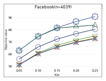
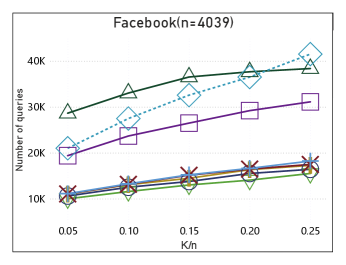
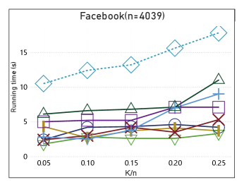
(a)              (b)              (c)

Figure 1: Performance of algorithms on Revenue Maximization for the Facebook dataset: (a) The objective values, (b) The number of queries and (c) their running time.

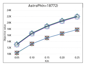
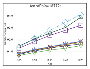
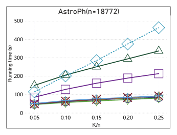
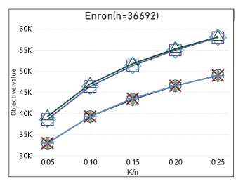
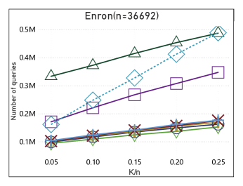
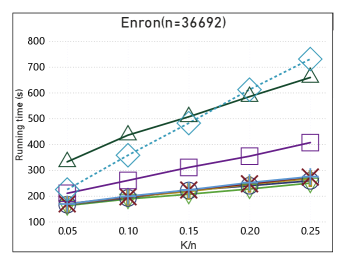
(a)              (b)              (c)

Figure 2: Performance of algorithms on Revenue Maximization for the AstroPh dataset: (a) The objective values, (b) The number of queries and (c) their running time.

(a)              (b)              (c)

Figure 3: Performance of algorithms on Revenue Maximization for the Enron dataset: (a) The objective values, (b) The number of queries and (c) their running time.

The results for the objective function values are presented in Figures 1a, 2a, and 3a. Among all methods, FastDrSub+ consistently achieves high objective function values, comparable to RLA and SMKRANACC, and outperforms the baseline FastDrSub variants with margins ranging from 1.2 to 1.4 times. Across all three datasets, FastDrSub+ maintains stable and competitive performance, with observed differences between high-performing algorithms being statistically insignificant. In the Facebook dataset, RLA shows slightly lower performance than FastDrSub+ and SMKRANACC at the 0.2 and 0.25 marks. For the FastDrSub algorithm with varying $\alpha$ values, the objective values are relatively similar in the AstroPh and Enron datasets due to their large size. In contrast, for the Facebook dataset, $\alpha=0.3$ yields the highest outcome among FastDrSub settings, while $\alpha=0.9$ gives the lowest, although the variation remains modest.

The results for the number of queries are shown in Figures 1b, 2b, and 3b. The algorithm FastDrSub+ requires more queries than FastDrSub variants, yet it generates significantly fewer queries than RLA and SMKRANACC. This efficiency is particularly evident in the Facebook and Enron datasets, where FastDrSub+ produces approximately 1.2 times fewer queries than RLA, indicating its favorable balance between performance and computational cost. The number of queries for FastDrSub remains consistent across different $\alpha$ values, with only slight variations across datasets.

Figures 1c, 2c, and 3c present the results for running time. The running time trends closely mirror the query counts, as expected. The FastDrSub algorithm with various $\alpha$ values achieves the shortest running times across all datasets, with minimal differences among $\alpha$ configurations. However, FastDrSub+ demonstrates a strong trade-off between solution quality and efficiency—it is faster than both RLA and SMKRANACC while delivering comparable objective values. In particular, on the AstroPh and Enron datasets, FastDrSub+ runs 1.5 to 2 times faster than RLA and SMKRANACC at $k/n=0.05$ and $k/n=0.25$, which demonstrates its practical efficiency.

6 Conclusion

This paper addresses the DrSMS problem, which generalizes the classical submodular maximization problem by incorporating diminishing returns over integer lattices. We introduced two efficient approximation algorithms designed to tackle this problem, with Algorithm FastDrSub providing an approximation ratio of $0.044$ and Algorithm FastDrSub+ achieving an even better ratio of $\frac{1}{4}-\epsilon$. Our theoretical analysis provides strong guarantees on both algorithms’ approximation quality and query complexity, demonstrating their effectiveness in various scenarios.

Furthermore, through extensive experimental evaluation, we showed that our algorithms outperform existing state-of-the-art methods, particularly in the context of Revenue Maximization applications, which leverage DR-submodular functions. The results highlight the practical value and efficiency of the proposed algorithms, making them suitable for large-scale problems where computational resources are limited.

Future work could further improve these algorithms’ scalability, explore additional problem formulations, and apply them to real-world applications with more complex constraints and objectives.

References

- (1) Bach, F.R.: Learning with submodular functions: A convex optimization perspective. Found. Trends Mach. Learn. 6(2-3), 145–373 (2013)
- (2) Badanidiyuru, A., Vondrák, J.: Fast algorithms for maximizing submodular functions. In: Proceedings of the twenty-fifth annual ACM-SIAM symposium on Discrete algorithms, pp. 1497–1514. SIAM (2014)
- (3) Buchbinder, N., Feldman, M.: Constrained submodular maximization via a nonsymmetric technique. Math. Oper. Res. 44(3), 988–1005 (2019)
- (4) Buchbinder, N., Feldman, M.: Constrained submodular maximization via new bounds for dr-submodular functions. In: Proceedings of the 56th Annual ACM Symposium on Theory of Computing, pp. 1820–1831 (2024)
- (5) Buchbinder, N., Feldman, M., Naor, J., Schwartz, R.: Submodular maximization with cardinality constraints. In: Proceedings of the twenty-fifth annual ACM-SIAM symposium on Discrete algorithms, pp. 1433–1452. SIAM (2014)
- (6) Calinescu, G., Chekuri, C., Pál, M., Vondrák, J.: Maximizing a submodular set function subject to a matroid constraint. In: International Conference on Integer Programming and Combinatorial Optimization, pp. 182–196. Springer (2007)
- (7) Chen, Y., Kuhnle, A.: Approximation algorithms for size-constrained non-monotone submodular maximization in deterministic linear time. In: A.K. Singh, Y. Sun, L. Akoglu, D. Gunopulos, X. Yan, R. Kumar, F. Ozcan, J. Ye (eds.) Proceedings of the 29th ACM SIGKDD Conference on Knowledge Discovery and Data Mining, KDD 2023, Long Beach, CA, USA, August 6-10, 2023, pp. 250–261. ACM (2023)
- (8) Crawford, V.G., Kuhnle, A., Thai, M.T.: Submodular cost submodular cover with an approximate oracle. In: K. Chaudhuri, R. Salakhutdinov (eds.) Proceedings of the 36th International Conference on Machine Learning, Proceedings of Machine Learning Research, vol. 97, pp. 1426–1435. PMLR (2019)
- (9) Das, A., Kempe, D.: Approximate submodularity and its applications: Subset selection, sparse approximation and dictionary selection. Journal of Machine Learning Research 19(3), 1–34 (2018)
- (10) Ene, A., Nguyen, H.: Parallel algorithm for non-monotone dr-submodular maximization. In: International Conference on Machine Learning, pp. 2902–2911. PMLR (2020)
- (11) Ene, A., Nguyen, H.L.: A reduction for optimizing lattice submodular functions with diminishing returns. arXiv e-prints pp. arXiv–1606 (2016)
- (12) Feige, U., Mirrokni, V.S., Vondrák, J.: Maximizing non-monotone submodular functions. SIAM Journal on Computing 40(4), 1133–1153 (2011)
- (13) Gharan, S.O., Vondrák, J.: Submodular maximization by simulated annealing. In: Proceedings of the twenty-second annual ACM-SIAM symposium on Discrete Algorithms, pp. 1098–1116. SIAM (2011)
- (14) Gottschalk, C., Peis, B.: Submodular function maximization on the bounded integer lattice. In: Approximation and Online Algorithms: 13th International Workshop, WAOA 2015, Patras, Greece, September 17-18, 2015. Revised Selected Papers 13, pp. 133–144. Springer (2015)
- (15) Goyal, A., Bonchi, F., Lakshmanan, L.V.S., Venkatasubramanian, S.: On minimizing budget and time in influence propagation over social networks. Social Netw. Analys. Mining 3(2), 179–192 (2013)
- (16) Guillory, A., Bilmes, J.A.: Simultaneous learning and covering with adversarial noise. In: L. Getoor, T. Scheffer (eds.) Proceedings of the 28th International Conference on Machine Learning, ICML, pp. 369–376. Omnipress (2011)
- (17) Gupta, A., Roth, A., Schoenebeck, G., Talwar, K.: Constrained non-monotone submodular maximization: Offline and secretary algorithms. In: International Workshop on Internet and Network Economics (2010)
- (18) Han, K., Cao, Z., Cui, S., Wu, B.: Deterministic approximation for submodular maximization over a matroid in nearly linear time. In: Advances in Neural Information Processing Systems 33: Annual Conference on Neural Information Processing Systems 2020, NeurIPS 2020, December 6-12, 2020, virtual (2020)
- (19) Han, K., Cui, S., Zhu, T., Zhang, E., Wu, B., Yin, Z., Xu, T., Tang, S., Huang, H.: Approximation algorithms for submodular data summarization with a knapsack constraint. Proceedings of the ACM SIGMETRICS conference on Measurement and Analysis of Computer Systems 5(1), 05:1–05:31 (2021)
- (20) Kuhnle, A.: Quick streaming algorithms for maximization of monotone submodular functions in linear time. In: International Conference on Artificial Intelligence and Statistics, pp. 1360–1368. PMLR (2021)
- (21) Kuhnle, A., Pan, T., Alim, M.A., Thai, M.T.: Scalable bicriteria algorithms for the threshold activation problem in online social networks. In: 2017 IEEE Conference on Computer Communications, INFOCOM, pp. 1–9. IEEE (2017)
- (22) Kuhnle, A., Smith, J.D., Crawford, V.G., Thai, M.T.: Fast maximization of non-submodular, monotonic functions on the integer lattice. In: J.G. Dy, A. Krause (eds.) Proceedings of the 35th International Conference on Machine Learning, ICML 2018, Stockholmsmässan, Stockholm, Sweden, July 10-15, 2018, Proceedings of Machine Learning Research, vol. 80, pp. 2791–2800. PMLR (2018)
- (23) Lai, L., Ni, Q., Lu, C., Huang, C., Wu, W.: Monotone submodular maximization over the bounded integer lattice with cardinality constraints. Discrete Mathematics, Algorithms and Applications 11(06), 1950075 (2019)
- (24) Lee, J., Mirrokni, V.S., Nagarajan, V., Sviridenko, M.: Maximizing nonmonotone submodular functions under matroid or knapsack constraints. SIAM Journal on Discrete Mathematics 23(4), 2053–2078 (2010)
- (25) Li, W.: Nearly linear time algorithms and lower bound for submodular maximization. preprint, arXiv:1804.08178 (2018). URL https://arxiv.org/abs/1804.08178
- (26) Li, W., Feldman, M., Kazemi, E., Karbasi, A.: Submodular maximization in clean linear time. In: Advances in Neural Information Processing Systems, pp. 7887–7897 (2022)
- (27) Li, Y., Li, M., Liu, Q., Zhou, Y.: Dr-submodular function maximization with adaptive stepsize. In: International Computing and Combinatorics Conference, pp. 347–358. Springer (2023)
- (28) Lin, H., Bilmes, J.A.: A class of submodular functions for document summarization. In: D. Lin, Y. Matsumoto, R. Mihalcea (eds.) The 49th Annual Meeting of the Association for Computational Linguistics: Human Language Technologies, Proceedings of the Conference, 19-24 June, 2011, Portland, Oregon, USA, pp. 510–520. The Association for Computer Linguistics (2011)
- (29) Mirzasoleiman, B., Badanidiyuru, A., Karbasi, A.: Fast constrained submodular maximization: Personalized data summarization. In: M. Balcan, K.Q. Weinberger (eds.) Proceedings of the 33nd International Conference on Machine Learning, ICML 2016, New York City, NY, USA, June 19-24, 2016, JMLR Workshop and Conference Proceedings, vol. 48, pp. 1358–1367. JMLR.org (2016). URL http://proceedings.mlr.press/v48/mirzasoleiman16.html
- (30) Mirzasoleiman, B., Karbasi, A., Badanidiyuru, A., Krause, A.: Distributed submodular cover: Succinctly summarizing massive data. In: C. Cortes, N.D. Lawrence, D.D. Lee, M. Sugiyama, R. Garnett (eds.) Advances in Neural Information Processing Systems 28, pp. 2881–2889 (2015)
- (31) Nemhauser, G.L., Wolsey, L.A., Fisher, M.L.: An analysis of approximations for maximizing submodular set functions—i. Mathematical programming 14, 265–294 (1978)
- (32) Norouzi-Fard, A., Bazzi, A., Bogunovic, I., Halabi, M.E., Hsieh, Y., Cevher, V.: An efficient streaming algorithm for the submodular cover problem. In: Advances in Neural Information Processing Systems 29, pp. 4493–4501 (2016)
- (33) Parambath, S.A.P., Vijayakumar, N., Chawla, S.: SAGA: A submodular greedy algorithm for group recommendation. In: S.A. McIlraith, K.Q. Weinberger (eds.) Proceedings of the Thirty-Second AAAI Conference on Artificial Intelligence, (AAAI-18), the 30th innovative Applications of Artificial Intelligence (IAAI-18), and the 8th AAAI Symposium on Educational Advances in Artificial Intelligence (EAAI-18), New Orleans, Louisiana, USA, February 2-7, 2018, pp. 3900–3908. AAAI Press (2018)
- (34) Pham, C.V., Duong, H.V., Thai, M.T.: Importance sample-based approximation algorithm for cost-aware targeted viral marketing. In: Computational Data and Social Networks - 8th International Conference, CSoNet 2019, Ho Chi Minh City, Vietnam, November 18-20, 2019, Proceedings, pp. 120–132 (2019). DOI 10.1007/978-3-030-34980-6“˙14. URL https://doi.org/10.1007/978-3-030-34980-6_14
- (35) Pham, C.V., Pham, D.V., Bui, B.Q., Nguyen, A.V.: Minimum budget for misinformation detection in online social networks with provable guarantees. Optimization Letters pp. 1–30 (2021)
- (36) Pham, C.V., Phu, Q.V., Hoang, H.X., Pei, J., Thai, M.T.: Minimum budget for misinformation blocking in online social networks. J. Comb. Optim. 38(4), 1101–1127 (2019)
- (37) Pham, C.V., Thai, M.T., Ha, D., Ngo, D.Q., Hoang, H.X.: Time-critical viral marketing strategy with the competition on online social networks. In: H.T. Nguyen, V. Snasel (eds.) Computational Social Networks, pp. 111–122. Springer International Publishing, Cham (2016)
- (38) Pham, C.V., Tran, T.D., Ha, D.T.K., Thai, M.T.: Linear query approximation algorithms for non-monotone submodular maximization under knapsack constraint. In: Proceedings of the Thirty-Second International Joint Conference on Artificial Intelligence, IJCAI 2023, 19th-25th August 2023, Macao, SAR, China, pp. 4127–4135. ijcai.org (2023)
- (39) Prajapat, M., Mutnỳ, M., Zeilinger, M.N., Krause, A.: Submodular reinforcement learning. In: Proc. International Conference on Learning Representations (ICLR) (2024)
- (40) Schiabel, A., Kungurtsev, V., Marecek, J.: Randomized algorithms for monotone submodular function maximization on the integer lattice. arXiv preprint arXiv:2111.10175 (2021)
- (41) Soma, T., Yoshida, Y.: A generalization of submodular cover via the diminishing return property on the integer lattice. In: C. Cortes, N.D. Lawrence, D.D. Lee, M. Sugiyama, R. Garnett (eds.) Advances in Neural Information Processing Systems 28, pp. 847–855 (2015)
- (42) Soma, T., Yoshida, Y.: Maximizing monotone submodular functions over the integer lattice. Mathematical Programming 172, 539–563 (2018)
- (43) Sun, X., Zhang, J., Zhang, S., Zhang, Z.: Improved deterministic algorithms for non-monotone submodular maximization. Theoretical Computer Science 984, 114293 (2024)
- (44) Sviridenko, M.: A note on maximizing a submodular set function subject to a knapsack constraint. Operations Research Letters 32(1), 41–43 (2004)
- (45) Vondrák, J.: Optimal approximation for the submodular welfare problem in the value oracle model. In: C. Dwork (ed.) Proceedings of the 40th Annual ACM Symposium on Theory of Computing, pp. 67–74. ACM (2008)