A Unified Spectrum for Turbulence in Microfluidic Flow

Abstract

We present a predictive master spectrum describing turbulence-like flows in microfluidic systems. Extending Pao’s viscous-range closure, the model introduces (i) an adaptive inertial-range slope dependent on measurable dimensionless numbers and (ii) a physics-specific cutoff that captures entropy-producing sinks such as electrokinetic forcing, compliant walls, active stresses, and interfacial tension. This formulation unifies turbulence regimes—electrokinetic, active, interfacial, and compressible—within one compact expression. Comparison with reported data reproduces both spectral slopes and dissipation cutoffs while requiring only global observables (velocity, viscosity, Taylor microscale, and forcing strength). The framework provides a design-level predictive tool for turbulent microflows prior to computationally heavy DNS or CFD.

Turbulence at the microscale combines the throughput advantages of microfluidics with the rapid mixing and energy redistribution typical of macroscopic turbulence. Experiments have shown broadband fluctuations at low Reynolds number $\mathrm{Re}<100$ generated by electrokinetic forcing under conductivity gradients [1], by active suspensions of bacteria or motor-protein bundles [2], by compliant microchannel walls [3], or by supersonic microjets [4]. To probe the laminar-to-turbulent transition, computational fluid dynamics (CFD) remains the de facto exploration tool, but its high cost limits iterative parameter screening for model optimization [5].To overcome this bottleneck, we propose a closed-form spectral law derived from classical turbulence theory and validate it against published experimental data.

The formulation originates from the incompressible Navier–Stokes equations under steady forcing, where nonlinear transfer redistributes energy across eddy scale but does not create or destroy energy. Averaging in Fourier space yields the spectral energy balance $\partial_{t}E(k)=T(k)+F(k)-2\nu k^{2}E(k)$, and at steady state (forcing and viscous effect are negligible) it gives a constant energy flux $\Pi(k)=\varepsilon$ across the inertial range. Dimensional arguments then recover the canonical scaling $E(k)=C_{K}\varepsilon^{2/3}k^{-m}$, with $m=5/3$ for classical turbulence. In microfluidic regimes, departures from this universal slope arise from finite Reynolds number($Re$), compressibility ($M$), activity ($\chi$), field coupling ($\beta$), interfacial stress ($I$), and electric forcing ($K$) expressed through a generalized slope function

$$m=\tfrac{5}{3}+a_{1}\!\tfrac{M^{2}}{1+M^{2}}+a_{2}\!\tfrac{\chi^{2}}{1+\chi^{2}}+a_{3}\!{\text{Re}}^{-1/4}+a_{4}\!\beta^{2}+a_{5}\!\tfrac{K^{2}}{1+K^{2}}+a_{6}\!\tfrac{I^{2}}{1+I^{2}}.$$ (1)

To represent dissipation, we extend Pao’s closure by combining viscous damping at the Kolmogorov wavenumber $k_{\eta}=(\varepsilon/\nu^{3})^{1/4}$ with an additional physics–specific cutoff $k_{\star}$, yielding

$$E(k)=C_{K}\,\varepsilon^{2/3}k^{-m}\exp\!\left[-\gamma_{v}\!\left(\frac{k}{k_{\eta}}\right)^{\alpha_{v}}\!\right]\exp\!\left[-\gamma_{p}\!\left(\frac{k}{k_{\star}}\right)^{\alpha_{p}}\!\right],$$ (2)

where the first exponential accounts for universal viscous losses and the second for entropy–producing mechanisms such as wall compliance, electrokinetic forcing, or active stresses.

For parameter evaluation, $\varepsilon$ follows the Taylor-microscale estimate [6, 7]

$$\varepsilon=15\nu u_{\mathrm{rms}}^{2}/\lambda^{2},$$ (3)

The smallest eddy scale $\eta=(\nu^{3}/\varepsilon)^{1/4}$ yields $k_{\eta}=1/\eta$.With experiment involving additional entropy-producing processes—such as elastic stresses in polymer solutions, activity in microbial suspensions, or compliance in soft-walled channels—a physics cutoff is incorporated, and the cutoff wavenumber $k_{\star}$ is assigned to the relevant microphysical scale (Table 1. The associated damping exponents $\gamma_{p}$ and $\alpha_{p}$ are tuned to capture the early onset of dissipation.

Table 1: Representative regimes and mechanisms defining the physics cutoff $k_{\star}$.

Regime	Mechanism	Definition
Compressible	Shock width $\delta_{s}$	$2\pi/\delta_{s}$
Active matter	Vortex size $R_{v}$	$2\pi/R_{v}$
Viscoelastic	Relax. length $\ell_{\mathrm{relax}}$	$2\pi/\ell_{\mathrm{relax}}$
Electrokinetic	Debye length $\lambda_{D}$	$2\pi/\lambda_{D}$
Soft-wall	Wall scale $\delta_{\mathrm{wall}}$	$2\pi/\delta_{\mathrm{wall}}$

Electrokinetic turbulence. The micro–electrokinetic turbulence (µEKT) experiments of Wang et al. [1] demonstrated turbulence generation by electrokinetic forcing across conductivity gradients. Using a laser-induced fluorescence photobleaching anemometer, they measured mean velocities of $U\approx 1.45$, 2.03, and 2.9 mm/s for $V_{\mathrm{pp}}=10$, 14, and 20 V, respectively. With $u_{\mathrm{rms}}\!\approx\!0.37U$, Kolmogorov scaling $\varepsilon\!\sim\!u_{\mathrm{rms}}^{3}/L$ ($L\!=\!240~\mu$m) yields $\eta\!\approx\!10$–5 µm and $k_{\eta}\!\approx\!10^{5}$–$2\times 10^{5}~\mathrm{m^{-1}}$. Despite low Reynolds numbers ($Re\!\approx\!0.4$–0.5), the predicted inertial–range slope remains consistent at $m\!\approx\!1.85$–1.86. The corresponding spectra, evaluated with $\gamma_{v}\!=\!1$ and $\alpha_{v}\!=\!4/3$, reproduce the experimental trends (Fig.1a). The predicted slopes ($m\!\approx\!1.85$–1.86) agree with experimental values within the reported 12% uncertainty for 14 and 20 V_pp ($m=1.68\pm 0.2$), validating the model at high applied voltage amplitude. At 10 V_pp, the measured spectrum steepens to $m\!\approx\!3$, consistent with the collapse of the inertial subrange and dominance of viscous and electrokinetic stress dissipation. The master equation, by construction, preserves a finite cascade and thus slightly overestimates $E(k)$ under weak forcing, where energy transfer is suppressed.

Shi et al. [8] examined electrokinetic–instability control by varying the electric Rayleigh number $Ra_{e}$ in a $100{\times}620~\mu$m² channel. For $Ra_{e}=2.9{\times}10^{6}$ and $4.5{\times}10^{6}$, the Taylor microscales were $\lambda=2.0{\times}10^{-5}$ m and $1.9{\times}10^{-5}$ m, giving $Re_{\lambda}=u_{\mathrm{rms}}\lambda/\nu\!\approx\!0.018$ and 0.016 ($\nu=10^{-6}$ m²/s). Using the isotropic estimate $\varepsilon=15\nu u_{\mathrm{rms}}^{2}/\lambda^{2}$ yields dissipation rates corresponding to $\eta\!\approx\!74$–76 µm and $k_{\eta}\!\approx\!1.3{\times}10^{4}$–$1.35{\times}10^{4}$ m^-1. Although $Re\!\sim\!1$, increasing $Ra_{e}$ strengthens electrokinetic forcing captured by the intensity parameter $K$, producing spectral slopes $m\!\approx\!1.82$ and 1.55 as $Ra_{e}$ rises (Fig.1b). However, the predicted slope ($m\!\approx\!1.82$) is different from the measured $m\!=\!7/5$ at high $Ra_{e}$, and the deviation arises from a regime shift in the cascade dynamics. The electric Rayleigh number, comparing electric forcing to viscous and diffusive dissipation, governs the balance between inertial– and scalar–driven transport. At low $Ra_{e}$, the flow retains an inertial–type cascade consistent with Wang et al., whereas at high $Ra_{e}$ enhanced conductivity fluctuations drive a scalar–dominated regime ($\text{electric forcing}\gg\text{viscous and diffusive dissipation}$ ), yielding a shallower slope. Incorporating the electrokinetic intensity parameter $K$ captures this transition ($K\gg 1$, $K^{2}/(1+K^{2})\rightarrow 1$), allowing the master spectrum to reproduce both inertial– and scalar–driven scaling within a unified framework.

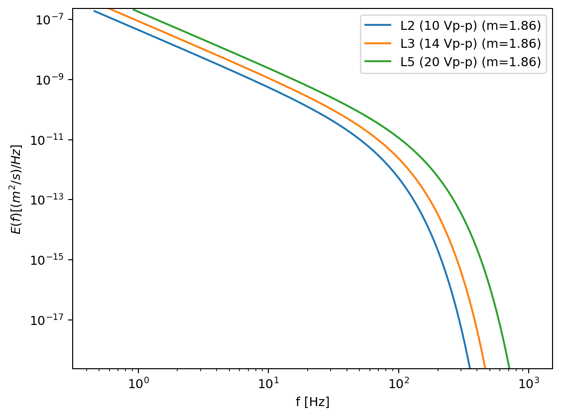
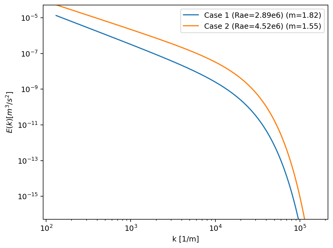
Figure 1: (a) Predicted spectra for electrokinetic turbulence at $V_{\mathrm{pp}}=10,14,20$ V [1]. (b) Predicted spectra for two electric Rayleigh numbers $Ra_{e}$ [8], where larger $Ra_{e}$ activates the electrokinetic term $K$ and reduces the slope toward $-7/5$. Parameters: $\gamma_{v}=1$, $\alpha_{v}=4/3$, $C_{K}=1$.

Interfacial turbulence. Padhan et al. [9] demonstrated interface–induced turbulence in binary–fluid mixtures, where interfacial stresses destabilize laminar cellular flows at low $Re$. Mapping their CHNS simulation ($2\pi$ domain) onto a $100~\mu$m microfluidic box gives $\lambda_{f}\!\approx\!25~\mu$m ($k_{f}\!\approx\!2.5{\times}10^{5}$ m^-1). Using water-like viscosity, the reference dissipation rate was defined as $\varepsilon_{0}=\nu^{3}k_{f}^{4}$. At the operating condition ($Ca=0.2$), the dissipation rate was $\varepsilon\simeq 0.5\,\varepsilon_{0}\approx 2.0\times 10^{3}\,\mathrm{m^{2}\,s^{-3}}$, yielding a Kolmogorov length scale $\eta\approx 4.7~\mu\mathrm{m}$ and corresponding cutoff wavenumber $k_{\eta}\approx 2.1\times 10^{5}~\mathrm{m^{-1}}$. At $Re\!\approx\!1$, inertia is negligible and turbulence is sustained by interfacial stresses characterized by the parameter $I$ ($I\gg 1$, $I^{2}/(1+I^{2})\rightarrow 1$), producing a spectral slope $m\!\approx\!4.65$. The normalized spectra computed with $\gamma_{v}\!=\!1$ and $\alpha_{v}\!=\!4/3$ (Fig. 2) reproduce the reported interface–driven cascade. At low Reynolds numbers, interfacial turbulence arises from stress–driven rather than inertial energy transfer. In this non–inertial regime, energy injection by interfacial or elastic stresses balances viscous dissipation locally, producing a steep spectral decay ($m\simeq 4.5$) consistent with stress–dominated cascades. The absence of inertial redistribution accelerates energy loss across scales, explaining the deviation from the Kolmogorov slope.

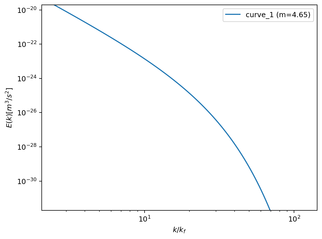
Figure 2: Predicted spectrum for interfacial turbulence [9]. Large $I$ yields $m\simeq 4.6$.

Active bacterial turbulence. Wensink et al. [2] showed that suspensions of motile bacteria self-organize into vortices and mesoscale turbulence even at very low Reynolds numbers. Using bacterial size $\ell\!\approx\!5~\mu$m and $U\!\approx\!100~\mu$m s^-1 gives $Re\!\approx\!5{\times}10^{-4}$ and $\varepsilon\!\sim\!U^{3}/\ell\!\approx\!2{\times}10^{-7}$ m²s^-3, with $\eta\!\approx\!5~\mu$m and $k_{\eta}\!\approx\!2{\times}10^{5}$ m^-1. The predicted slope $m\!=\!8/3$ captures the steep active-stress cascade. Spectra computed with $\gamma_{v}\!=\!1$, $\alpha_{v}\!=\!4/3$, and a physics cutoff ($\gamma_{p}\!=\!1$, $\alpha_{p}\!=\!1$, $k_{\star}\!=\!1.3{\times}10^{5}$ m^-1) reproduce the measured mesoscale energy peak (Fig. 3).

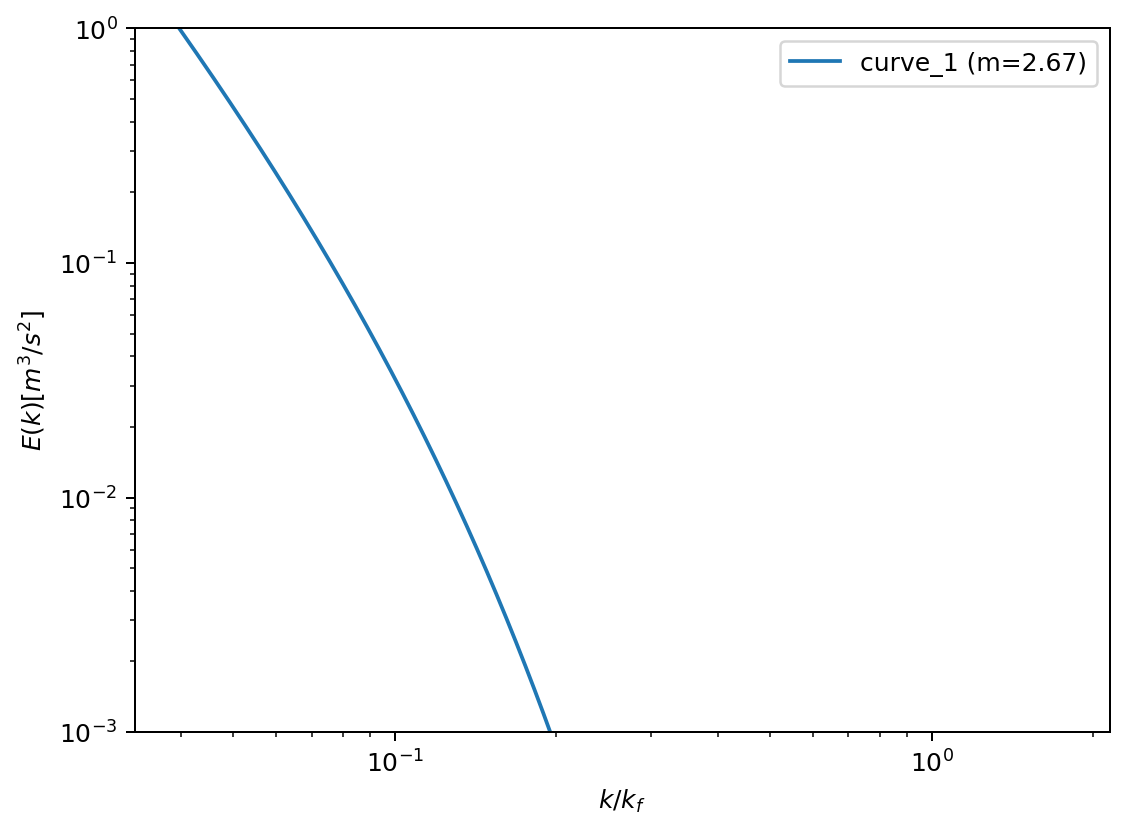
Figure 3: Predicted spectrum for active bacterial turbulence [10]. $m\simeq 8/3$, $\gamma_{p}=1$, $\alpha_{p}=1$, $k_{\star}=1.3\times 10^{5}$ m^-1.

Slope prediction. In addition to empirical curve fitting, direct extraction of dimensionless parameters from published studies enables rapid, quantitative validation of the predictive model. Table 2 summarizes the benchmark cases spanning four representative turbulence-like regimes—soft-wall elasticity, hydrodynamic oscillation, compressible plasma flow, and active stress injection—each revealing how the spectral exponent $m$ systematically departs from the Kolmogorov value of $5/3$ in response to distinct physical constraints (Figure4).

The fluidic oscillator [11], actuated through periodic jet generation in CFD simulations, sustains turbulence-like motion purely via hydrodynamic instabilities. As no external coupling or additional dissipation mechanisms are present, the cascade retains the canonical $k^{-5/3}$ scaling, reducing the spectrum to the classical Kolmogorov–Pao form that characterizes inertial–viscous balance. Soft-wall elasticity [3] has been demonstrated to induce turbulence-like mixing in microfluidic channels, evidenced by uniform pH distribution and convergence of particle counts. Elastic wall deformation enables continuous exchange between kinetic and potential energy, introducing an additional entropy-producing sink that modifies the cascade dynamics. This compliance is captured through the physics-specific cutoff $k_{\star}=2\pi/\delta_{\mathrm{wall}}$, representing the wall deformation scale, and results in a steepened spectrum relative to the inertial–viscous baseline.

The supersonic plasma system [12] sustains compressible turbulence at a Mach number of approximately 5.4 through the collision of counter-propagating plasma jets generated by laser ablation. In this regime, shock formation introduces an additional dissipation channel beyond viscous losses, producing a steepened energy spectrum relative to the incompressible case. The corresponding physics cutoff ($k_{\star}=2\pi/\delta_{s}$, where $\delta_{s}$) represents the scale at which kinetic energy is converted into heat through shock dissipation. This behavior confirms that compressibility modifies the inertial cascade by coupling acoustic and vortical modes, thereby enhancing spectral decay beyond the Kolmogorov prediction. The exceptionally high dissipation rate reflects the macroscopic nature and strong compressibility of the plasma flow—far exceeding typical microfluidic conditions—thereby intensifying energy conversion within the shock-dominated cascade.

The active micromachine system [2], composed of self-propelled rods or motor–protein–driven filaments, sustains turbulence through continuous active stress injection in addition to inertial transfer. Because energy is supplied at a characteristic mesoscale rather than at large flow scales, the cascade bypasses the conventional inertial range and dissipates prematurely. This behavior is captured by the physics cutoff $k_{\star}=2\pi/R_{v}$, where $R_{v}$ represents the typical vortex size, reflecting the localized energy injection and rapid spectral decay characteristic of active turbulence.

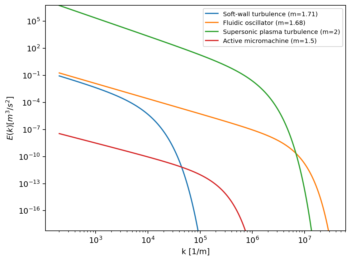
Figure 4: Slope prediction on distinct physical mechanism: soft-wall elasticity, hydrodynamic oscillation, supersonic plasma turbulence, and active micromachine flow.

Table 2: Parameters used for spectral prediction.

Group	Case	$\varepsilon$ (m2/s3)	$m$	$\gamma_{v}$	$\alpha_{v}$	$k_{\eta}$ (m-1)	$\gamma_{p}$	$\alpha_{p}$	$k_{\star}$ (m-1)
Experimental Fitting	Micro-EKT (Wang et al.)	$3.1{\times}10^{-6}$–$2.5{\times}10^{-5}$	1.86	1	1.33	$1$–$2{\times}10^{5}$	0	0	0
	Quad-cascade EKT (Shi et al.)	$3.0$–$3.3{\times}10^{-2}$	1.82–1.55	1	1.33	$1.3$–$1.4{\times}10^{4}$	0	0	0
	Active fluid (Wensink et al.)	$2.0{\times}10^{-7}$	2.67	1	1.33	$2.0{\times}10^{5}$	1	1	$1.3{\times}10^{5}$
	Interfacial (Padhan et al.)	$2.0{\times}10^{3}$	4.65	1	1.33	$2.1{\times}10^{5}$	0	0	0
Slope Prediction	Soft-wall turbulence (Kumaran et al.)	$2.29{\times}10^{4}$	1.71	1	1.33	$3.89{\times}10^{5}$	1	1	$3.14{\times}10^{3}$
	Fluidic oscillator (Laín et al.)	$5.12{\times}10^{4}$	1.68	1	1.33	$2.99{\times}10^{6}$	0	2	$1.19{\times}10^{4}$
	Supersonic plasma (Meinecke et al.)	$1.10{\times}10^{17}$	2.00	1	1.33	$2.80{\times}10^{6}$	1	1	$5.00{\times}10^{5}$
	Active micromachine (Thampi et al.)	$1.00{\times}10^{-6}$	1.50	1	1.33	$1.57{\times}10^{5}$	1	1	$1.57{\times}10^{5}$

The predicted energy spectrum provides a compact framework for interpreting turbulence across regimes and guiding experimental design. The spectral slope defines the cascade law: a Kolmogorov regime follows the canonical $m=5/3$ exponent, while interfacial-driven turbulence produces a steeper $m\!\approx\!4.5$. The slope and curve shape thus determine characteristic scales and mixing lengths, and any deviation between predicted and measured slopes signals additional physics—such as activity or elasticity—beyond a purely inertial cascade.

The dissipation rate $\varepsilon$ quantifies the energy flux across scales and, through $\eta=(\nu^{3}/\varepsilon)^{1/4}$, fixes the smallest eddy size. Higher $\varepsilon$ permits smaller eddies and enhanced mixing but increases energy consumption and velocity gradients. Using the global balance $\varepsilon=\Delta P\,U/L$, dissipation links directly to the required pressure drop, revealing the increase in mixing efficiency simultaneously increase systemic shear stress, which affects specimen viability and elevates energy cost of the device. Thus, spectral prediction provides a quantitative tool for optimizing design of microfluidic systems.

Cutoff scales visible in the spectrum define both natural viscous limits ($k_{\eta}$) and tunable design constraints ($k_{\star}$) associated with bacterial size, polymer relaxation length, or interfacial thickness. Shifts in cutoff position reflect how dissipation and physical coupling reshape the accessible eddy hierarchy. The high-$k$ ($k\geq k_{\eta}$) termination of the curve, where viscous or physics-specific damping dominates, indicates how efficiently energy is removed relative to its injection rate.

Finally, the integral $\int_{0}^{\infty}E(k)\,dk=\tfrac{1}{2}\langle u^{2}\rangle$ provides the total turbulent kinetic energy, offering a consistency check between predicted cascade dynamics and measured input power.

We present a unified spectral framework that links electrokinetic, interfacial, soft-wall, active, and compressible microfluidic turbulence within a single predictive law. Extending Pao’s closure with a generalized slope and physics-specific cutoff, the model captures both universal inertial scaling and entropy-producing microscale effects. Validation across four decades in dissipation rate and three in cutoff scale shows that elasticity, compressibility, and activity systematically reshape the cascade relative to the Kolmogorov–Pao baseline. The preliminary validation demonstrates that the model serves as a rapid diagnostic for mixing, dissipation, and scale-dependent energy transfer, providing a first-stage predictive tool before resorting to computationally intensive simulations.

References

- Wang et al. [2016] G. Wang, F. Yang, and W. Zhao, Physical Review E 93, 013106 (2016).
- Thampi et al. [2016] S. P. Thampi, A. Doostmohammadi, T. N. Shendruk, R. Golestanian, and J. M. Yeomans, Science Advances 2, e1501854 (2016).
- Kumaran and Bandaru [2016] V. Kumaran and P. Bandaru, Chemical Engineering Science 149, 156 (2016).
- Aniskin et al. [2015] V. M. Aniskin, S. G. Mironov, A. A. Maslov, and I. S. Tsyryulnikov, Microfluidics and Nanofluidics 19, 621 (2015).
- Ebner and Wille [2023] P. Ebner and R. Wille, in Proceedings of the 2023 26th Euromicro Conference on Digital System Design (DSD) (IEEE, 2023).
- Taylor [1935] G. I. Taylor, Proceedings of the Royal Society of London. Series A, Mathematical and Physical Sciences 151, 421 (1935).
- Batchelor [1953] G. K. Batchelor, The Theory of Homogeneous Turbulence (Cambridge University Press, Cambridge, UK, 1953).
- Shi et al. [2025] Y. Shi, J. Pang, Y. Zhu, M. Zeng, K. Nan, Y. Chen, C. Zhang, T. Zhao, C. Zhang, G. Jing, K. Wang, J. Bai, and W. Zhao, Physics of Fluids 37, 025151 (2025).
- Padhan et al. [2024] N. B. Padhan, D. Vincenzi, and R. Pandit, Physical Review Fluids 9, L122401 (2024).
- Wensink et al. [2012] H. H. Wensink, J. Dunkel, S. Heidenreich, K. Drescher, R. E. Goldstein, H. Löwen, and J. M. Yeomans, Proceedings of the National Academy of Sciences 109, 14308 (2012).
- Laín et al. [2022] S. Laín, M. Romagnoli, M. Coello, D. Cabaleiro, and A. Rivas, Applied Sciences 12, 9305 (2022).
- Meinecke et al. [2019] J. Meinecke, P. Tzeferacos, A. R. Bell, R. Bingham, R. Crowston, et al., Nature Communications 10, 1174 (2019).