Neural network initialization with nonlinear characteristics and information on spectral bias

Abstract

Initialization of neural network parameters, such as weights and biases, has a crucial impact on learning performance; if chosen well, we can even avoid the need for additional training with backpropagation. For example, algorithms based on the ridgelet transform or the SWIM (sampling where it matters) concept have been proposed for initialization. On the other hand, it is well-known that neural networks tend to learn coarse information in the earlier layers. The feature is called spectral bias. In this work, we investigate the effects of utilizing information on the spectral bias in the initialization of neural networks. Hence, we propose a framework that adjusts the scale factors in the SWIM algorithm to capture low-frequency components in the early-stage hidden layers and to represent high-frequency components in the late-stage hidden layers. Numerical experiments on a one-dimensional regression task and the MNIST classification task demonstrate that the proposed method outperforms the conventional initialization algorithms. This work clarifies the importance of intrinsic spectral properties in learning neural networks, and the finding yields an effective parameter initialization strategy that enhances their training performance.

I Introduction

The fields of machine learning and artificial intelligence are deeply connected to physics, as evidenced by the fact that neural networks won the 2024 Nobel Prize. However, its significant computational cost during both training and utilization has also become problematic from an environmental impact perspective. In utilizing trained neural networks, techniques such as pruning and quantization are widely employed to improve efficiency; see the recent reviews in [1, 2]. Here, we focus on the training stage of the neural networks from the perspective of sampling, which would also be interesting in statistical physics.

It has been widely known that neural networks exhibit high versatility and strong approximation capability [3, 4]. Their nonlinearity yields powerful and practical learned networks in various applications in image recognition, natural language processing, and speech recognition. However, as the number of hidden layers increases, the number of parameters grows exponentially, leading to longer training times [5, 6, 7, 8]. Since training involves non-convex optimization, there is also a risk of local minima and stagnation in flat regions. These issues highlight the critical importance of parameter initialization.

Since conventional backpropagation requires huge computational costs, other types of neural networks have been proposed. One example is the extreme learning machine (ELM) [9, 10]. The ELM is a training algorithm for a feedforward neural network with only one hidden layer. In the ELM, one randomly chooses hidden node parameters, and the learning process is applied only to the output layer through simple linear regression. Hence, the learning process for the ELM is fast and efficient; for details of the ELM, see the recent review paper [11]. However, even shallow neural networks suffer from unstable learning.

To address this problem, one approach is to modify the random initialization of parameters. That is, one could employ some theories and data for the parameter initialization. For example, we transform shallow neural networks into an integral representation and apply a sampling method called oracle sampling [12, 13]. In the oracle sampling algorithm, hidden-layer parameters are sampled from a ridgelet-transform-based distribution, and the conventional linear regression determines output parameters. In [14], we revisited the oracle sampling algorithm from the perspective of importance sampling, which leads to an initialization method that demonstrates higher performance than the original one. These approaches achieve near-trained performance without backpropagation, and the theoretical framework is also used in discussions of deep networks, utilizing, for example, harmonic analysis on groups [15, 16, 17]. However, the practical sampling method is limited to single hidden-layer models.

The SWIM (sampling where it matters) algorithm [18] was proposed in a different context from the ridgelet-transform-based initialization method, which enables the generation of parameters for deep networks. The SWIM algorithm constructs hidden-layer weights and biases directly from input data pairs, determining all parameters, except those of the output-layer, via sampling. The output layer is then fitted by linear regression, allowing high performance even in deep networks without gradient-based training. The SWIM algorithm has also been applied to graph neural networks and higher-order partial differential equations, demonstrating its potential as a non-gradient learning method based on random features [19, 20, 21].

In the present paper, we propose a parameter initialization method that employs the nature of nonlinear characteristics and information on spectral bias. In the SWIM algorithm, we find that the nonlinearity used in the activation function is controllable by changing hyperparameters for each hidden layer. It is possible to reflect the information of the spectral bias in the setting of the hyperparameters. We confirm that the proposed initialization method improves the performance in a simple one-dimensional example and the MNIST datasets.

The remainder of this paper is structured as follows. Section II provides a brief overview of the SWIM algorithm and presents simple numerical experiments concerning spectral bias. Section III discusses the nonlinearity and hyperparameters in the SWIM algorithm and proposes a parameter initialization method to incorporate information on spectral bias. Section IV presents numerical results demonstrating the effectiveness of the proposed method. Section V presents some considerations and conclusions.

II Background knowledge

II.1 Sampling Where It Matters (SWIM)

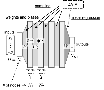
Figure 1: The parameter initialization in the SWIM algorithm. The parameters in the hidden layers are initialized by using the dataset. Only the parameters in the output layer are learned by the conventional linear regression.

The SWIM algorithm was proposed in [18], which initializes the parameters of a neural network. Figure 1 shows the framework of the SWIM algorithm. In the SWIM algorithm, directly sampled pairs of input data initialize the parameters of all layers except the output layer. Then, the conventional linear regression between outputs of the neural network and the target data determines the parameters of the output layer.

Of course, it is possible to apply the learning based on the gradient descent method after the initialization by the SWIM algorithm. However, as we will see in Sect. IV, only the initialization by the SWIM yields reasonable performance. Hence, the SWIM algorithm reduces the computational cost of the learning process.

Below, we provide a brief explanation of the SWIM algorithm, with the flow outlined in Algorithm 1. Let $X\subset\mathbb{R}^{D}$ be the input space with the Euclidean norm $\|\cdot\|$ and the inner product $\langle\cdot,\cdot\rangle$. Furthermore, let $\Phi$ be a neural network with $L$ hidden layers; the activation function is $\phi:\mathbb{R}\rightarrow\mathbb{R}$, and the network parameters in the $l$-th layer is $\{W_{l},\bm{b}_{l}\}$ for $l=1$ to $l=L+1$. For $\bm{x}\in X$, we write a result from the activation function with the $i$-th element $[W_{l}\Phi^{(l-1)}(\bm{x})-\bm{b}_{l}]_{i}$ as $[\Phi^{(l)}(\bm{x})]_{i}=\phi([W_{l}\Phi^{(l-1)}(\bm{x})-\bm{b}_{l}]_{i})$, where $\Phi^{(0)}(\bm{x})=\bm{x}$. The number of nodes in the $l$-th layer is denoted as $N_{l}$ with $N_{0}=D$; $N_{L+1}$ is the output dimension. $W_{l}$ has a matrix form, and we write the $i$-th row of $W_{l}$ as $\bm{w}_{l,i}$; the $i$-th element of the vector $\bm{b}_{l}$ is denoted as $b_{l,i}$.

Here, assume that we have a sufficiently large dataset. In the SWIM algorithm, an important step is the sampling procedure from a dataset. Let $\big\{\big(\bm{x}^{(1)}_{0,i},\bm{x}^{(2)}_{0,i}\big)\big\}^{N_{l}}_{i=1}$ for $l=1,\ldots,L$ be the sampled pairs of data points over $X\times X$. That is, to determine the weight and bias of a single node in a layer, we sample a pair consisting of two data points; we avoid using the same data as the pair, i.e., $\bm{x}^{(1)}_{0,i}\neq\bm{x}^{(2)}_{0,i}$. Using the sampled data pair, the weight and bias are initialized as follows:

$$\bm{w}_{l,i}=s_{1}\frac{\widetilde{\bm{x}}^{(2)}_{l-1,i}-\widetilde{\bm{x}}^{(1)}_{l-1,i}}{||\widetilde{\bm{x}}^{(2)}_{l-1,i}-\widetilde{\bm{x}}^{(1)}_{l-1,i}||^{2}},\quad b_{l,i}=\langle\bm{w}_{l,i},\widetilde{\bm{x}}^{(1)}_{l-1,i}\rangle+s_{2},$$ (1)

where $s_{1},s_{2}\in\mathbb{R}$ are hyperparameters, and $\widetilde{\bm{x}}^{(j)}_{l-1,i}=\Phi^{(l-1)}(\bm{x}^{(j)}_{0,i})$ for $j=1,2$. The output layer is selected by the conventional linear regression, and the parameters $W_{L+1}$ and $\bm{b}_{L+1}$ are set as follows:

$$W_{L+1},\bm{b}_{L+1}=\underset{\widetilde{W}_{L+1},\widetilde{\bm{b}}_{L+1}}{\operatorname{argmin}}\,\mathcal{L}(\widetilde{W}_{L+1}\Phi^{L}(X)-\widetilde{\bm{b}}_{L+1},Y),$$ (2)

where $\mathcal{L}$ is the loss function, which is usually set as a mean squared error.

Algorithm 1 The SWIM algorithm

1: Constant: $\varepsilon\in\mathbb{R}_{>0}$, $\varsigma\in\mathbb{N}_{>0},L\in\mathbb{N}_{>0},\{N_{l}\in\mathbb{N}_{>0}\}_{l=1}^{L+1},s_{1},s_{2}\in\mathbb{R}$

2: Data: $X=\{\bm{x}_{i}\in\mathbb{R}^{D}\}_{i=1}^{M}$, $Y=\{\bm{f}(\bm{x}_{i})=\bm{y}_{i}\in\mathbb{R}^{N_{L+1}}\}_{i=1}^{M}$

3: for $l=1,2,\ldots,L$ do

4:  $\widetilde{M}_{l}\leftarrow\varsigma\cdot\left\lceil\frac{N_{l}}{M}\right\rceil\cdot M$

5:  $P^{(l)}_{i}\leftarrow 0$   for   $i=1,\dots,\widetilde{M}_{l}$.

6:  $\widetilde{X}=\left\{(\bm{x}_{0,i}^{(1)},\bm{x}_{0,i}^{(2)})\mid\Phi^{(l-1)}(\bm{x}_{0,i}^{(1)})\neq\Phi^{(l-1)}(\bm{x}_{0,i}^{(2)})\right\}_{i=1}^{\widetilde{M}_{l}}$ $\quad\sim$ Uniform $(X\times X)$  (where $\Phi^{(0)}(\bm{x})=\bm{x}$)

7:  for $i=1,2,\ldots,\widetilde{M}_{l}$ do

8:   $\widetilde{\bm{x}}_{l-1,i}^{(1)}\leftarrow\Phi^{(l-1)}(\bm{x}_{0,i}^{(1)})$,  $\widetilde{\bm{x}}_{l-1,i}^{(2)}\leftarrow\Phi^{(l-1)}(\bm{x}_{0,i}^{(2)})$

9:   $\widetilde{\bm{y}}_{i}^{(1)}\leftarrow f(\bm{x}_{0,i}^{(1)})$,  $\widetilde{\bm{y}}_{i}^{(2)}\leftarrow f(\bm{x}_{0,i}^{(2)})$

10:   $\displaystyle P_{i}^{(l)}\leftarrow\frac{\|\widetilde{\bm{y}}_{i}^{(2)}-\widetilde{\bm{y}}_{i}^{(1)}\|_{L^{\infty}}}{\max\{\|\widetilde{\bm{x}}_{l-1,i}^{(2)}-\widetilde{\bm{x}}_{l-1,i}^{(1)}\|,\varepsilon\}}$

11:  end for

12:  $W_{l}\in\mathbb{R}^{N_{l}\times N_{l-1}}$, $b_{l}\in\mathbb{R}^{N_{l}}$

13:  for $i=1,2\ldots,N_{l}$ do

14:   Sample $(\bm{x}_{0,i}^{(1)},\bm{x}_{0,i}^{(2)})$ from $\widetilde{X}$ with replacement and with probability proportional to $\{P_{i}^{(l)}\}$;

15:   $\widetilde{\bm{x}}_{l-1,i}^{(1)}\leftarrow\Phi^{(l-1)}(\bm{x}_{0,i}^{(1)})$,  $\widetilde{\bm{x}}_{l-1,i}^{(2)}\leftarrow\Phi^{(l-1)}(\bm{x}_{0,i}^{(2)})$

16:   $\displaystyle\bm{w}_{l,i}\leftarrow s_{1}\frac{\widetilde{\bm{x}}_{l-1,i}^{(2)}-\widetilde{\bm{x}}_{l-1,i}^{(1)}}{\|\widetilde{\bm{x}}_{l-1,i}^{(2)}-\widetilde{\bm{x}}_{l-1,i}^{(1)}\|^{2}}$, $\,\,b_{l,i}\leftarrow\langle\bm{w}_{l,i},\widetilde{\bm{x}}_{l-1,i}^{(1)}\rangle+s_{2}$

17:  end for

18:  $[\Phi^{(l)}(\bm{x}_{k})]_{i}\leftarrow\phi([W_{l}\Phi^{(l-1)}(\bm{x}_{k})-\bm{b}_{l}]_{i})$       for $k=1,2,\dots,M$ and $i=1,2,\dots,N_{l}$

19: end for

20: $\displaystyle W_{L+1},\bm{b}_{L+1}\leftarrow\underset{\widetilde{W}_{L+1},\widetilde{\bm{b}}_{L+1}}{\operatorname{argmin}}\,\mathcal{L}(\widetilde{W}_{L+1}\Phi^{(L)}(X)-\widetilde{\bm{b}}_{L+1},Y)$

21: return $\{W_{l},\bm{b}_{l}\}_{l=1}^{L+1}$

Here, we should focus on the choice of the data pairs. In [18], there is the following notice, “putting emphasis on points that are close and differ a lot with respect to the output of the true function works well.” Then, the following sampling framework at each layer is employed in the SWIM algorithm. First, we prepare enough data pairs for the $l$-th layer, i.e., $\big\{\big(\bm{x}^{(1)}_{0,i},\bm{x}^{(2)}_{0,i}\big)\big\}_{i=1}^{\widetilde{M}_{l}}$; when $M$ is the number of training data sets, we set $\widetilde{M}_{l}=\varsigma\cdot\left\lceil\frac{N_{l}}{M}\right\rceil\cdot M$ with a hyperparameter $\varsigma\in\mathbb{N}_{>0}$. Note that we avoid the choice with $\Phi^{(l-1)}\big(\bm{x}_{0,i}^{(1)}\big)\neq\Phi^{(l-1)}\big(\bm{x}_{0,i}^{(2)}\big)$. Second, we assign the following quantity to each data pair:

$$P_{i}^{(l)}=\frac{\|\widetilde{\bm{y}}_{i}^{(2)}-\widetilde{\bm{y}}_{i}^{(1)}\|_{L^{\infty}}}{\max\{\|\widetilde{\bm{x}}_{l-1,i}^{(2)}-\widetilde{\bm{x}}_{l-1,i}^{(1)}\|,\varepsilon\}},$$ (3)

where $\widetilde{\bm{x}}_{l-1,i}^{(j)}=\Phi^{(l-1)}\big(\bm{x}_{0,i}^{(j)}\big)$ and $\widetilde{\bm{y}}_{i}^{(j)}=f\big(\bm{x}_{0,i}^{(j)}\big)$ for $j=1,2$, and $\varepsilon>0$ for $l\in\{1,2\ldots,L\}$ and $\varepsilon=0$ for $l=1$. Note that the $L^{\infty}$ norm is used for the numerator in Eq. (3), which returns the maximum element of $\widetilde{\bm{y}}_{i}^{(2)}-\widetilde{\bm{y}}_{i}^{(1)}$. The parameter $\varepsilon$ is necessary to avoid a division by zero. Then, the weights and biases are determined via Eq. (1) by using a data pair sampled probability proportional to $\{P_{i}^{(l)}\}$.

II.2 Spectral bias in a neural network for a toy problem

Fully connected neural networks are one of the simplest types of neural networks whose nodes are fully connected to the nodes in the next layer. For the fully connected neural networks, it is known that low-frequency components are learned preferentially in the initial layers of the networks. This characteristic is called spectral bias; see, for example, [22].

Table 1: Setting in the preliminary experiment to see spectral bias.

Input dimension	1
# of hidden layers	3
# of nodes in each hidden layer	124
Output dimension	1
# of epochs	1000
Activation function	$\sin$
Optimization method	Adam
Loss function	Mean Squared Error
Learning rate	$0.01$

Here, we demonstrate the characteristic of the spectral bias with a simple neural network and a toy problem. We learn a one-dimensional function $f(x)=\sin(4\pi x)$ with fully connected neural networks with three hidden layers. The experimental setting is shown in Table 1.

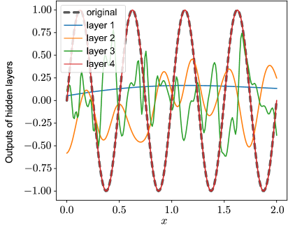
Figure 2: (Color online) Outputs of the learned fully connected neural network for each layer. The horizontal axis is the input $x$, and the vertical axis represents values with a matrix product of the weights of the final layer $W_{L+1}$ to each hidden layer. The dashed curve corresponds to the original function $f(x)$. Since the learning is effectively finished, the output of the final layer, i.e., layer 4, matches the original function $f(x)$ well.

To investigate the role of each hidden layer, we directly connect the final weight matrix $W_{L+1}$ to each hidden layer and visualize its output. Figure 2 depicts the results. The outputs of layer 4, i.e., the final outputs of the neural network, match the original function $f(x)$ well, confirming that the learning was successful. We can see that the curves gradually become more complex in the order of layers 1, 2, and 3. Hence, the feature of low-frequency components is learned in the early stage of the network; this fact indicates that the fully connected neural network exhibits the property of spectral bias.

III Proposal to employ information on spectral bias

III.1 Revisit on the role of hyperparameters $s_{1}$

As denoted in Sect. II.A, the original SWIM algorithm has two hyperparameters, $s_{1}$ and $s_{2}$, used to determine the weights and biases, respectively; see Eq. (1). In [18], these values are determined with the following discussions.

The weight parameter $\bm{w}_{l,i}$ is determined by the data pair, as in Eq. (1). Intuitively, the weight vector is in the direction of the difference between the two points, and the bias is defined as the inner product from a reference point in that direction. As a result, the weights are placed at input locations where the activation function performs a meaningful nonlinear transformation.

To see this construction, for simplicity, we here take

$$\widetilde{\bm{x}}^{(2)}_{l-1,i}=-\widetilde{\bm{x}}^{(1)}_{l-1,i}.$$ (4)

Then, we have

$$\bm{w}_{l,i}=-\frac{s_{1}}{2}\frac{\widetilde{\bm{x}}^{(1)}_{l-1,i}}{||\widetilde{\bm{x}}^{(1)}_{l-1,i}||^{2}}$$ (5)

and

$$b_{l,i}=-\frac{s_{1}}{2}\frac{1}{||\widetilde{\bm{x}}^{(1)}_{l-1,i}||^{2}}\langle\widetilde{\bm{x}}^{(1)}_{l-1,i},\widetilde{\bm{x}}^{(1)}_{l-1,i}\rangle+s_{2}=-\frac{s_{1}}{2}+s_{2}.$$ (6)

Hence, the value of the activation function on $\widetilde{\bm{x}}^{(1)}_{l-1,i}$ becomes

$$\phi\left(\langle\bm{w}_{l,i},\widetilde{\bm{x}}^{(1)}_{l-1,i}\rangle-b_{l,i}\right) =\phi\left(\left\langle-\frac{s_{1}}{2}\frac{\widetilde{\bm{x}}^{(1)}_{l-1,i}}{||\widetilde{\bm{x}}^{(1)}_{l-1,i}||^{2}},\widetilde{\bm{x}}^{(1)}_{l-1,i}\right\rangle-\frac{s_{1}}{2}+s_{2}\right)$$

$$=\phi\left(-s_{1}+s_{2}\right).$$ (7)

Note that the activation function takes $\phi(s_{2})$ on $\widetilde{\bm{x}}^{(2)}_{l-1,i}$. For example, we consider $\tanh$ as the activation function. Then, if we set $s_{1}=\ln 3$ and $s_{2}=(\ln 3)/2$, the activation function takes $-0.5$ and $+0.5$ on $\widetilde{\bm{x}}^{(1)}_{l-1,i}$ and $\widetilde{\bm{x}}^{(2)}_{l-1,i}$, respectively. Hence, these hyperparameters effectively utilize the nonlinear region of $\tanh$. The similar discussions were used to determine the values of the hyperparameters in [18].

From the above discussions, we conjecture that $s_{1}$ is more relevant than $s_{2}$ because $s_{2}$ is related only to the bias term. To investigate the effects of these hyperparameters, we performed several preliminary numerical experiments, which suggested that $s_{1}$ largely affects the final performance. By contrast, $s_{2}$ has little effect on performance. Hence, we focus primarily on the hyperparameter $s_{1}$ in the following discussion.

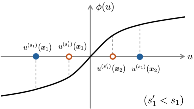
Figure 3: (Color online) Example of different choices with the parameter for $s_{1}$. Even if the same data pair $(\bm{x}_{1},\bm{x}_{2})$ is used, the degree of nonlinearity utilized varies depending on the parameters. When $s^{\prime}_{1}<s_{1}$, the small parameter $s^{\prime}_{1}$ utilizes only the portion where the activation function changes abruptly.

To discuss the role of $s_{1}$, we define the following quantity:

$$u^{(s_{1})}(\bm{x})=\left\langle s_{1}\frac{\widetilde{\bm{x}}^{(2)}_{l-1,i}-\widetilde{\bm{x}}^{(1)}_{l-1,i}}{||\widetilde{\bm{x}}^{(2)}_{l-1,i}-\widetilde{\bm{x}}^{(1)}_{l-1,i}||^{2}},\bm{x}\right\rangle,$$ (8)

which is one of the arguments in the activation function, i.e., $\phi(u^{(s_{1})}(\bm{x})+b)$. As a pedagogical example, we will consider the role of parameters here using $\tanh$ as the activation function. Figure 3 shows the shape of the activation function. Since the parameter $s_{1}$ varies the weight parameter vector $\bm{w}_{l,i}$ in Eq. (7), the actual coordinate $u^{(s_{1})}(\bm{x})$ depends on the value of $s_{1}$ even for the same input vector $\bm{x}$. In Fig. 3, the same data points, $\bm{x}_{1}$ and $\bm{x}_{2}$, yield different coordinates $u^{(s_{1})}(\bm{x}_{1})$ and $u^{(s_{1})}(\bm{x}_{2})$

From the above discussions, we have the following ideas. That is, the smaller parameter $s^{\prime}_{1}$ tends to focus on regions near the origin. Hence, only a limited range of the activation function is mainly utilized. Since various inputs are within a narrow range, subtle differences in inputs are difficult to distinguish, which corresponds to low-frequency information.

By contrast, the larger parameter $s_{1}$ tends to utilize a larger region of the activation function. This means that the nonlinearity of the activation function is effectively available. Hence, the activation function can capture the subtle differences in various inputs.

III.2 Proposal of new parameter initialization method

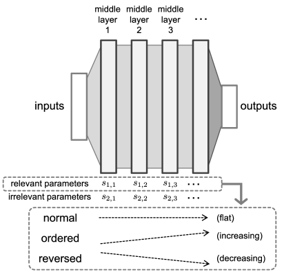
Figure 4: Framework to include the information on spectral bias. The relevant hyperparameter $s_{1}$ can vary across hidden layers. The “ordered” is the proposed method, in which $s_{1,l}$ gradually increases with the layer index $l$. By contrast, $s_{1,l}$ gradually decreases in the “reversed” method. The “normal” corresponds to the original SWIM algorithm in which $s_{1,l}$ is constant.

According to the above discussions, we propose a framework to include the information on the spectral bias. In the original SWIM algorithm, the scale factor $s_{1}$ is set to a constant value for all hidden layers. Since $s_{1}$ controls the scale of the activation function, we change $s_{1}$ for each intermediate layer, as in Fig. 4; we write the hyperparameter for the $l$-th layer as $s_{1,l}$.

The discussion on spectral bias suggests that it would be better to process coarse information in the early layers and deal with fine details in the later layers. Hence, we propose the following ordered setting:

$$\bm{s}_{1}=[s_{1,1},s_{1,2},\cdots,s_{1,L}],$$

$$\bm{s}_{2}=[s_{2,1},s_{2,2},\cdots,s_{2,L}]=\frac{1}{2}\bm{s}_{1},$$ (9)

where $s_{1,1}\leq s_{1,2}\leq s_{1,3}\leq\cdots\leq s_{1,L}$. While we tried several settings for $s_{2}$, there were no significant differences. Hence, we employed the above setting.

In Fig. 4, we depict two other methods; the reversed method has the reversed order of $s_{1,l}$, which is designed to capture high-frequency components in the initial layers and gradually decrease the scale factor in deeper layers. The normal is the original SWIM algorithm; $s_{1,l}$ is constant for all the indices $l$.

IV Numerical Experiments

In this section, we demonstrate the effects of the information on the spectral bias. Here, we compare the proposed method with the original SWIM algorithm and the reversed method.

We checked various settings in preliminary numerical experiments; we set the parameters to $\varepsilon=0.01$, $\varsigma=10$, and the activation function to $\phi(\cdot)=\sin(\cdot)$ in all the numerical results in this paper. In addition, for the original SWIM algorithm, we show numerical results with $s_{1,i}=\ln{3},s_{2,i}=(\ln{3})/2$ for all index $i$.

IV.1 Regression task on 1D data

We first consider a regression task on 1D data. We use the following target function:

$$f(x)= \sin(2\cdot 2\pi x)+0.3\sin(20\cdot 2\pi x)$$

$$+0.1\sin(30\cdot 2\pi x)+0.05\sin(40\cdot 2\pi x).$$ (10)

We sample 200 data points uniformly from the interval $[0,2]$ and use these points as the input data. The target values are computed using the above function. Table 2 shows the experimental setting. The number of hidden layers is $3$, and all the hidden layers have the same number of nodes; we change the number of nodes in the experiments. The hyperparameter $\bm{s}_{1}$ is set as $\{s_{1,1},s_{1,2},s_{1,3},s_{1,4}\}=\{0.5,7,13.5,20\}$; only the increasing tendency is crucial, and there is no reason to select these hyperparameter values. We tried several hyperparameters, and all the results have the same tendency. The above hyperparameter value appears to yield reasonable results, and we present the numerical results for the corresponding hyperparameter values. In addition, note that we do not apply the backpropagation procedure; only the samplings and the conventional linear regression on the final layer are employed.

Table 2: Experimental setting for the one-dimensional problem.

Input dimension	1
# of hidden layers	3
# of nodes in each hidden layer	(variable)
Output dimension	1

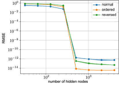
Figure 5: The RMSE and standard deviation of the neural network outputs for each method, averaged over 5 runs. The horizontal axis is the number of nodes in each hidden layer, and the vertical axis corresponds to the RMSE. While there are error bars depicted by the standard deviation, it is difficult to see them because they are too small.

Figure 5 depicts the root mean square error (RMSE) of the output of the neural network for each method. In the normal method, the original SWIM algorithm is used, and the hyperparameters are common across all layers. In the reversed method, the hyperparameter $\bm{s}_{1}$ has the reversed order, i.e., $\{s_{1,1},s_{1,2},s_{1,3},s_{1,4}\}=\{20,13.5,7,0.5\}$; each element of the vector $\bm{s}_{2}$ is half the value of that of $\bm{s}_{1}$.

When the number of nodes in the hidden layers is small, there are insufficient nodes for learning, which results in poor accuracy across all methods. When there is a sufficient number of nodes, Fig. 5 indicates that the proposed method (ordered) achieves the lowest RMSE values compared to the original SWIM algorithm (normal) and the reversed method (reversed) in the case of a large number of nodes.

To discuss the reason for the good performance of the proposed method, we next see the role of each hidden layer, as in Fig. 2. Figure 6 depicts the output of the neural network for each method; connecting each hidden layer to the final layer yields the output values. Here, we show the results for the neural network with 1024 nodes in all hidden layers. One of the remarkable features in Fig. 6 is that the value of the vertical axis of the ordered method is close to the target function. However, the values of the vertical axis of the normal and the reversed methods are not close to the target function. Furthermore, the ordered method captures the low-frequency components in the initial layers, which would allow the network to learn effectively.

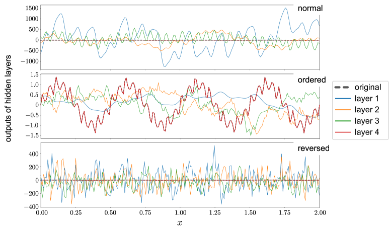
Figure 6: The output values computed by connecting the final layer directly to each hidden layer. The dashed lines correspond to the true function $f(x)$ in Eq. (10). The values of layer 4 are the outputs of the neural network, and hence, they mostly match the true function $f(x)$. Note that due to the large scale of the vertical axes in the top (normal) and bottom (reversed) figures, the true function $f(x)$ appears almost constant in these figures.

IV.2 Classification task on MNIST

Next, we apply the proposed method to a classification task on the MNIST dataset [23, 24]. The number of training images of handwritten digits is 15,000, and that of test images is 10,000. Table 3 shows the experimental setting. The hyperparameter $\bm{s}_{1}$ is set as $\{s_{1,1},s_{1,2},s_{1,3},s_{1,4}\}=\{0.01,0.173,0.337,0.5\}$. Again, note that we do not apply the backpropagation procedure; only the samplings and the conventional linear regression on the final layer are employed.

Table 3: Experimental setting for the MNIST problem.

Input dimension	784 (28$\times$28 pixels)
# of hidden layers	3
# of nodes in each hidden layer	(variable)
Output dimension	10 (10 digits)

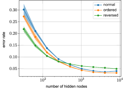
Figure 7: The error rate and standard deviation of the neural network outputs for each method, averaged over 5 runs. The horizontal axis is the number of nodes in each hidden layer, and the vertical axis corresponds to the error rate.

Figure 7 depicts the error rate of the neural network outputs for each method. In the classification task, the proposed method (ordered) achieves the lowest error rates in cases of large numbers of nodes. Hence, even in the high-dimensional inputs, the information on the spectral bias improves the performance.

Here, we comment on why the proposed method (ordered) performs worse than the reversed method when the number of nodes in the hidden layers is small. As we discussed in Sec. III. A, a small value of the hyperparameter $s_{1}$ mainly focuses on coarse information (low-frequency). Since a small number of nodes in the hidden layers cannot deal with the coarse information sufficiently, we observe poor performance.

By contrast, a larger $s_{1}$ allows us to deal with detailed information. Note that the small number of nodes in the hidden layers corresponds to rough information processing. Then, it would be natural that the rough information processing of “detailed information” yields better performance than the rough information processing of “coarse information.”

Of course, the above discussion is valid only for the small number of nodes in the hidden layers, where the error rate is inherently high and performance is poor. As far as we checked with several different examples, activation functions and the hyperparameter settings, the information on the spectral bias works well when there is a large number of nodes in the hidden layer.

V Conclusion

The data-driven initialization of weights and biases enables us to avoid learning with conventional backpropagation. As for the initialization, we proposed a method to exploit the information on the spectral bias. The crucial point is the role of the hyperparameter $s_{1}$ in the original SWIM algorithm, which changes the role of nonlinearity in the activation function. The gradual change of the hyperparameter allows us to capture the low-frequency components in the hidden layers in the early stage. We demonstrated the effects of the information of the spectral bias with several numerical experiments; the proposed method outperforms the original SWIM method and the reversed-order method in both regression and classification tasks.

There are several remaining tasks in the future. First, applying this approach to other types of neural networks, such as convolutional neural networks (CNNs) and recurrent neural networks (RNNs), is an important future task. Second, further investigation of how to set the scaling factor $s_{1}$ is also important. As far as we checked, the gradual change of parameters improves performance. However, the degree of improvement varies depending on the settings. Optimal parameter settings may exist. Furthermore, while this study varied parameters according to layer depth, practical adjustments could be possible; for example, the parameter change within the same hidden layer could be effective in some situations.

Studies utilizing features such as spectral bias in sampling-based initialization techniques have just started. We hope this study will contribute to the exploration of efficient learning methods for future neural networks.

- [1] T. Liang, J. Glossner, L. Wang, S. Shi, and X. Zhang, Neurocomputing 461, 370 (2021).
- [2] H. Cheng, M. Zhang and J. Q. Shi, IEEE Transactions on Pattern Analysis & Machine Intelligence 46, 10558 (2024).
- [3] G. Cybenko, Math. Cont. Signals Syst. 2, 303 (1989).
- [4] A. Barron, IEEE Transactions on Information Theory 39, 930 (1993).
- [5] S. Sun, W. Chen, L. Wang, X. Liu, and T.-Y. Liu, Proc. AAAI Conf. Artificial Intelligence, 2016, p. 2066.
- [6] V. Sze, Y.-H. Chen, T.-J. Yang, and J. Emer, Proc. AAAI Conf. Artificial Intelligence, 2017, p. 2295.
- [7] K.A. Sankararaman, S. De, Z. Xu, W.R. Huang, and T. Goldstein, Proc. Machine Learning Research, 2020, p. 8469.
- [8] M.G.M Abdolrasol, S.M.S Hussain, T.S. Ustun, M.R. Sarker, M.A. Hannan, R. Mohamed, J.A. Ali, S. Mekhilef, and A. Milad, Electronics 10, 2689 (2021).
- [9] G.-B. Huang, Q.-Y. Zhu, and C.-K. Siew, Proc. 2004 IEEE Int. Joint Conf. Neural Networks, 2004, p. 985.
- [10] G.-B. Huang, Q.-Y. Zhu, and C.-K. Siew, Neurocomputing 70, 489 (2006).
- [11] J. Wang, S. Lu, S.-H. Wang, and Y.-D. Zhang, Multimed. Tools Appl. 81, 41611 (2022).
- [12] N. Murata, Neural Networks 9, 947 (1996).
- [13] S. Sonoda and N. Murata, Lecture Notes in Computer Science 8681, 539 (2014).
- [14] H. Homma and J. Ohkubo, J. Phys. Soc. Jpn. 93, 124001 (2024).
- [15] S. Sonoda and N. Murata, J. Machine Learn. Res. 20, 1 (2019).
- [16] S. Sonoda, Y. Hashimoto, I. Ishikawa, and M. Ikeda, Proc. NeurIPS 2023 Workshop on Symmetry and Geometry in Neural Representations (2023).
- [17] S. Sonoda, Y. Hashimoto, I. Ishikawa, M. Ikeda, Proc. Int. Conf. Machine Learning (2025).
- [18] E. L. Bolager, I. Burak, C. Datar, Q. Sun, and F. Dietrich, Advances in Neural Information Processing Systems, 36, 63075 (2023).
- [19] C. Datar, T. Kapoor, A. Chandra, Q. Sun, E.L. Bolager, I. Burak, A. Veselovska, M. Fornasier, F. Dietrich, arXiv:2405.20836.
- [20] Z. Nikita, C. Thomas and G. Lukas, Proc. Int. Conf. Machine Learning (2025).
- [21] R. Atamert, D. Chinmay, C. Ana and D. Felix, arXiv:2506.06558.
- [22] N. Rahaman et al., Proc. Machine Learning Research 97, 5301 (2019).
- [23] Y. LeCun, L. Bottou, Y. Bengio, and P. Haffner, Proc. IEEE 86, 2278 (1998).
- [24] L. Deng, IEEE Signal Process. Mag. 29, 141 (2012).