Magnetic-type Love number differentiating quark stars from neutron stars

Abstract

The quark star (QS) is a hypothetical and yet undiscovered stellar object, and its existence would mark a paradigm shift in research on nuclear and quark matter. Although compactness is a well-known signature for distinguishing between two branches of QSs and neutron stars (NSs), some QSs can overlap with NSs in the radius-mass plane. To manifest their evident differences, we investigate the tidal properties of QSs and NSs. We then find that the magnetic-type Love number is a robust indicator for differentiating between QSs and NSs, whereas the electric-type one is insufficient when QSs and NSs have similar masses and radii. Finally, we show that gravitational waves from binary star mergers can be sensitive to differences between QSs and NSs to the detectable level.

Introduction:

Strange quark matter (SQM) could be more stable than hadronic matter at zero pressure [1, 2, 3]. According to this SQM hypothesis, compact stellar objects composed entirely of quark matter, i.e., quark stars (QSs), can exist in the universe [4, 5, 6, 7, 8, 9, 10]. Numerous attempts are made (see Refs. [11, 12] for $f$- and $g$-mode oscillations, Ref. [13] for a critical discussion on seismic vibrations, Ref. [14] for machine learning, Ref. [15] for core-crust oscillation, etc.) and more exotic scenarios are discussed [16, 17, 18, 19], but no convincing support for the QS existence has been established. Recently, QS studies have widely attracted interest since the compact object in the supernova remnant, HESS J1731-347, may have $M=0.77^{+0.20}_{-0.17}M_{\odot}$ and $R=10.4^{+0.86}_{-0.78}\,\mathrm{km}$ [20], where $M$ and $R$ are the mass and the radius of the star and $M_{\odot}$ is the solar mass, implying that it is either the lightest neutron star (NS) or it may be the QS candidate. On the large-mass side, the $2.6^{+0.07}_{-0.10}M_{\odot}$ secondary in GW190814 [21] has also been discussed as a QS candidate [19].

If the equation of state (EoS) is derived from the fundamental theory of the Strong Interaction, that is, quantum chromodynamics (QCD), the inner structures of compact stellar objects composed of strongly interacting matter can be solved uniquely. Such procedures are well-established for studying NS properties. However, QCD at high density suffers from the notorious sign problem (see Ref. [22, 23] for a review), and any reliable EoS cannot be obtained from the first-principles method. Thus, there is no direct way to justify or falsify the SQM hypothesis from QCD, and we must rely on astrophysical data to extract EoS information experimentally.

Thanks to advances in both perturbative QCD at high density [24, 25] and astrophysical observation analyses [26, 27, 28, 29], the distribution of masses and radii of the NSs can constrain the EoS well up to $\sim 5$ times the nuclear saturation density. In this way, it is likely that a core of quark matter exists in massive NSs [30], which can be further tested by the future gravitational-wave (GW) measurements [31, 32, 33, 34, 35]. Furthermore, GW170817 supposedly originates from the merger of binary NSs, and the inferred value of the dimensionless tidal deformability, $\Lambda$, provides additional constraints on the likely EoS candidate [36, 37].

In the near future, more and more GW signals will be detected and a useful set of $\{M,\,k^{\mathrm{el}}_{2}\}$ will be accumulated, where $k^{\mathrm{el}}_{2}$ is the electric-type quadrupolar Love number leading to $\Lambda$ [38]. This can be translated into a set of $\{M,\,R\}$. In the optimistic scenario, some $M$ and/or $R$ far apart from the $M$-$R$ branch of the NSs would be a clear signature for the QS. However, the QSs may have a distribution in the larger mass region, depending on the formation mechanism and the stability scenario, and their preferred mass may be around $\gtrsim 1.4M_{\odot}$ like the NSs or even heavier as discussed in the GW190814 context [39, 14, 40, 41, 42, 43, 44, 45]. In other words, some objects that are considered to be massive NSs could be the QSs masquerading as the NSs (see Ref. [46] for related discussions on a hybrid star). If we find any indicator to distinguish between the QSs and the NSs in the mass region $\gtrsim 1.4M_{\odot}$, it would crucially enhance our chance to discover the QS candidates.

To disentangle similarity between massive QSs and NSs, we need to introduce another observable in addition to $\{M,\,R\}$ or $\{M,\,k^{\mathrm{el}}_{2}\}$. An immediate candidate is the combination of all, i.e., $\{M,\,R,\,k^{\mathrm{el}}_{2}\}$. However, this idea does not work well. To obtain $\{M,\,R,\,k^{\mathrm{el}}_{2}\}$, it is necessary to determine each of them independently, which requires simultaneous observations of electromagnetic and gravitational waves from the same star. There is no such simultaneous observation, and the prospect of future observation will be extremely limited.

One may think that the Love-$C$ relation [47] complements $\{M,\,R,\,k^{\mathrm{el}}_{2}\}$, but this approach does not work, either. The conventional Love-$C$ relation is derived from various NS EoSs, and thus, only the NS combinations of $\{M,\,R,\,k^{\mathrm{el}}_{2}\}$ should inevitably be concluded as a result of the Love-$C$ relation applied to $\{M,\,R\}$ or $\{M,\,k^{\mathrm{el}}_{2}\}$. To overcome this, one may find a broader Love-$C$ relation that can fit the EoSs of both QSs and NSs. In that case, however, such a broader Love-$C$ relation is no longer precise, and the uncertainty diminishes the resolution to distinguish between the QSs and the NSs from $\{M,\,R,\,k^{\mathrm{el}}_{2}\}$.

In our work, we propose that the magnetic-type quadrupolar Love number, $k^{\mathrm{mag}}_{2}$, is a new distinguishing indicator. We note that $k^{\mathrm{mag}}_{2}$ carries information independent of $k^{\mathrm{el}}_{2}$ imprinting on the GW signals, and in our convention, the definition of $k^{\mathrm{mag}}_{2}$ follows from Refs. [48, 49]. The magnetic-type Love number, $k^{\mathrm{mag}}_{2}$, is estimated from the given EoS, and it characterizes a response of a self-gravitating body to external magnetic tidal fields corresponding to parity-odd perturbations [50].

We shall demonstrate that $k^{\mathrm{mag}}_{2}$ is a promising indicator for a wide variety of SQM EoSs. In the literature [47, 51, 52], some SQM EoSs were adopted from phenomenological models for the QSs, and we extensively generalize the analysis using 28 independent QS EoSs. For comparison, we employ 26 different NS EoSs. In this way, we estimate the possible ranges of $k^{\mathrm{el}}_{2}$ and $k^{\mathrm{mag}}_{2}$ belonging to the QS and NS branches, respectively. Our results show that, even when the QS and NS branches stay close in the $M$-$R$ plane or the $M$-$k^{\mathrm{el}}_{2}$ plane, two branches are well separated in the $M$-$k^{\mathrm{mag}}_{2}$ plane.

Construction of SQM EoSs:

Our working hypothesis is that QSs consist entirely of SQM [6, 7, 8, 10]. Since the surface of QSs, defined by $p=0$, is composed of SQM, such EoSs have a nonzero surface energy density; $\varepsilon_{0}\neq 0$. The value of $\varepsilon_{0}$ should be large enough to stabilize SQM as the true ground state. We construct a broad range of SQM EoS candidates in a way that satisfies physical requirements. Specifically, we adopt the following prescriptions to generate SQM EoS candidates:

• Asymptotic Boundary Condition $(\varepsilon\geq\varepsilon_{1})$: For high enough energy densities above a threshold, $\varepsilon_{1}$, the pressure is assumed to be given by the pQCD calculation, i.e., $p=p_{\text{pQCD}}(\varepsilon)$.

• Polytropic Interpolation $(\varepsilon_{0}\leq\varepsilon\leq\varepsilon_{1})$: Between $\varepsilon_{0}$ at the stellar surface and the threshold $\varepsilon_{1}$, a single polytropic parametrization is assumed as $p=K\bigl(\varepsilon-\varepsilon_{0}\bigr)^{\alpha}$.

There are four parameters, $K$, $\alpha$, $\varepsilon_{0}$, and $\varepsilon_{1}$, and they are constrained by the smoothness condition and the causality condition. The meaning of these parameters is illustrated in Fig. 1.

The smoothness condition assumes neither first- nor second-order phase transition at $\varepsilon=\varepsilon_{1}$. This means that neither $p$ nor $dp/d\varepsilon$ has a discontinuity at $\varepsilon=\varepsilon_{1}$. That is,

$$K(\varepsilon-\varepsilon_{0})^{\alpha}\Bigr|_{\varepsilon=\varepsilon_{1}} =p_{\text{pQCD}}(\varepsilon)\Bigr|_{\varepsilon=\varepsilon_{1}}\,,$$ (1)

$$\frac{d}{d\varepsilon}K(\varepsilon-\varepsilon_{0})^{\alpha}\Bigr|_{\varepsilon=\varepsilon_{1}} =\frac{dp_{\text{pQCD}}(\varepsilon)}{d\varepsilon}\Bigr|_{\varepsilon=\varepsilon_{1}}\,.$$ (2)

These conditions fix $K$ and $\alpha$ for given $\varepsilon_{0}$ and $\varepsilon_{1}$.

The causality condition reads that the speed of sound, $c_{s}^{2}=dp/d\varepsilon$, never exceeds the speed of light, i.e., unity in the present units, for any energy density. Since $p=p_{\text{pQCD}}(\varepsilon\geq\varepsilon_{1})$ is consistent with causality, this condition restricts a physical range of $\varepsilon_{0}$ and $\varepsilon_{1}$. For example, if the window between $\varepsilon_{0}$ and $\varepsilon_{1}$ is too narrow, the causality condition would be violated.

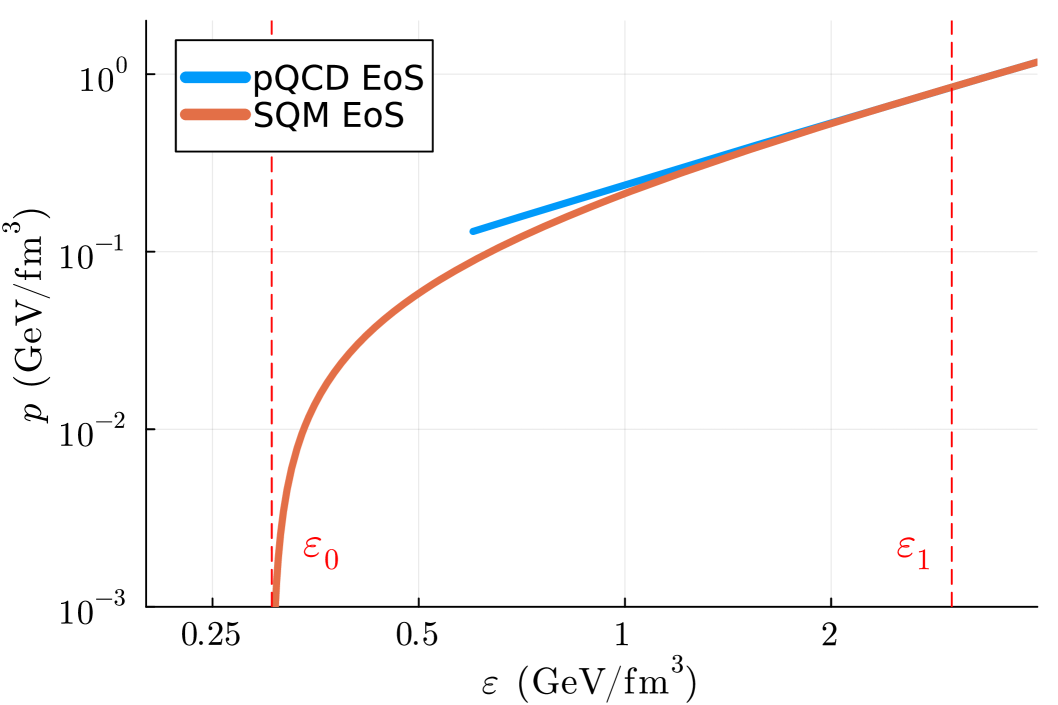
Figure 1: Parametrization of the SQM EoS with $\varepsilon_{0}$ and $\varepsilon_{1}$. The red curve represents the resulting SQM EoS for given $\varepsilon_{0}$ and $\varepsilon_{1}$. The slope is adjusted so that the polytropic EoS is smoothly connected to the pQCD EoS at $\varepsilon=\varepsilon_{1}$.

To generate concrete SQM EoSs based on the aforementioned construction, we need to fix $\varepsilon_{0}$ and $\varepsilon_{1}$. The allowed range of $\varepsilon_{0}$ is determined as follows. According to the MIT bag model, $\varepsilon_{0}$ is related to the bag pressure, $B$, as $\varepsilon_{0}=4B$ [53]. Then, $B$ must have a lower bound to prevent atomic nuclei from decaying into non-strange QM. The minimum value of $B$ is estimated to be $B=B_{\mathrm{min}}\simeq$57.5\text{\,}\mathrm{M}\mathrm{e}\mathrm{V}\mathrm{/}\mathrm{f}\mathrm{m}^{3}$$ [2, 54], leading to $\varepsilon_{0}\gtrsim 4B_{\mathrm{min}}\simeq$230\text{\,}\mathrm{M}\mathrm{e}\mathrm{V}\mathrm{/}\mathrm{f}\mathrm{m}^{3}$$. It is more difficult to constrain the upper bound on $\varepsilon_{0}$, but we do not need it in the present context. If $\varepsilon_{0}$ is excessively large, the gap between QSs and NSs in the $M$-$R$ plane would become wider. Then, it would be easier to differentiate them even without referring to the tidal properties. In addition to $\varepsilon_{0}$, we must set $\varepsilon_{1}$ in such a way as not to violate the causality condition. Because $dp/d\varepsilon=K\alpha(\varepsilon-\varepsilon_{0})^{\alpha-1}$, it is clear that $\alpha>1$ is a necessary condition; otherwise, $c_{s}$ diverges at $\varepsilon=\varepsilon_{0}$.

Quark Matter EoS	$\varepsilon_{0}\ (\mathrm{GeV/fm^{3}})$	$\varepsilon_{1}-\varepsilon_{0}\ (\mathrm{GeV/fm^{3}})$
NJL $(g_{V}^{(0)},H^{(0)})$	$0.23$	$1$
NJL $(g_{V}^{(0)},H^{(0)})$	$0.23$	$2$
NJL $(g_{V}^{(0)},H^{(0)})$	$0.23$	$3$
NJL $(g_{V}^{(0)},H^{(0)})$	$0.3052$	$1$
NJL $(g_{V}^{(0)},H^{(0)})$	$0.3052$	$2$
NJL $(g_{V}^{(0)},H^{(0)})$	$0.3052$	$3$
NJL $(g_{V}^{(1)},H^{(1)})$	$0.23$	$1$
NJL $(g_{V}^{(1)},H^{(1)})$	$0.23$	$2$
NJL $(g_{V}^{(1)},H^{(1)})$	$0.23$	$3$
NJL $(g_{V}^{(1)},H^{(1)})$	$0.3052$	$1$
NJL $(g_{V}^{(1)},H^{(1)})$	$0.3052$	$2$
NJL $(g_{V}^{(1)},H^{(1)})$	$0.3052$	$3$
NJL $(g_{V}^{(2)},H^{(2)})$	$0.23$	$1$
NJL $(g_{V}^{(2)},H^{(2)})$	$0.23$	$2$
NJL $(g_{V}^{(2)},H^{(2)})$	$0.23$	$3$
NJL $(g_{V}^{(2)},H^{(2)})$	$0.3052$	$1$
NJL $(g_{V}^{(2)},H^{(2)})$	$0.3052$	$2$
NJL $(g_{V}^{(2)},H^{(2)})$	$0.3052$	$3$
pQCD	$0.23$	$2$
pQCD	$0.23$	$3$
pQCD	$0.23$	$4$
pQCD	$0.23$	$5$
pQCD	$0.23$	$\infty$
pQCD	$0.3052$	$3$
pQCD	$0.3052$	$4$
pQCD	$0.3052$	$5$
pQCD	$0.3052$	$\infty$

Table 1: Parameters for the SQM EoSs. The quark matter part is given by the NJL model in Ref. [55] with several coupling choices, $g_{V}^{(0)}/G=0.5$, $g_{V}^{(1)}/G=0.8$, $g_{V}^{(2)}/G=1.0$, $H^{(0)}/G=1.4$, $H^{(1)}/G=1.5$, $H^{(2)}/G=1.6$, where $G$ represents the scalar-pseudoscalar coupling. Another choice of the quark matter part is the pQCD-based EoS with $X=4$ using the notation in Ref. [56]. For the choice of $\varepsilon_{0}=4B$, $0.23\text{\,}\mathrm{G}\mathrm{e}\mathrm{V}\mathrm{/}\mathrm{f}\mathrm{m}^{3}$ is taken from Refs. [2, 54] and $0.3052\text{\,}\mathrm{G}\mathrm{e}\mathrm{V}\mathrm{/}\mathrm{f}\mathrm{m}^{3}$ is taken from Ref. [57]. For the choice of $\varepsilon_{1}\to\infty$, practically, $\varepsilon_{1}-\varepsilon_{0}=10^{3}\,\mathrm{GeV/fm^{3}}$ is chosen.

More specifically, for the QSs, three types of the Nambu-Jona-Lasinio (NJL) models [58, 59, 60, 61] are employed to describe the quark matter part with the model parameters given in Ref. [55]. For each choice of the vector interaction $g_{V}$ and the diquark interaction $H$, we change $\varepsilon_{0}$ and $\varepsilon_{1}$ as listed in Table 1. Also, a pQCD-based EoS is employed with $X=4$, where $X$ is a parameter in the running strong coupling in Ref. [56]. Furthermore, for reference in later discussions, we adopt the MIT bag model with $B=$57.5\text{\,}\mathrm{M}\mathrm{e}\mathrm{V}\mathrm{/}\mathrm{f}\mathrm{m}^{3}$$ for the QS EoS [2, 54].

The preparation of the NS EoSs is simple. We take typical nuclear EoSs from the polytropic parametrization listed in Ref. [62]. There are 34 EoSs in the original listing, but we exclude AP1, AP2, AP3, AP4, ENG, WFF1, WFF2, BBB2, and GS1a, which violate the causality condition within the energy region up to eight times the energy density at nuclear saturation. We also note that some EoSs we adopt cannot explain massive NSs with $M\sim 2\,M_{\odot}$. The purpose of considering various NS EoSs is to estimate the typical uncertainty width in $R$, $k^{\mathrm{el}}_{2}$, and $k^{\mathrm{mag}}_{2}$, and to this end, we do not have to care too much about the quality of EoSs. Alternatively, we could have generated random EoSs and utilized the posterior probability under physical conditions in the Bayesian analysis. However, the results should be consistent in the end. In addition to the listed EoSs, as a guide of eyes, we overlay the results from the Crossover EoS taken from Ref. [34].

Indistinguishability of massive QSs and NSs:

As shown in Fig. 2, the $M$-$R$ curves for QSs and NSs intersect at masses around $M\gtrsim 1.4\,M_{\odot}$. It is impossible to distinguish QSs from NSs solely based on the $M$-$R$ observation in this mass region.

For these QS and NS EoSs, we compute $k^{\mathrm{el}}_{2}$ to make a plot in Fig. 3. As seen in Fig. 3, we find that the QSs and NSs curves intersect in the mass region around $M\gtrsim 1.4\,M_{\odot}$. Again, it is difficult to distinguish between QSs and NSs with the knowledge about $M$-$k^{\mathrm{el}}_{2}$ observations in this mass region. Our results that $k^{\mathrm{el}}_{2}$ takes similar values for QSs and NSs in the high-mass range are consistent with the discussions in Ref. [52].

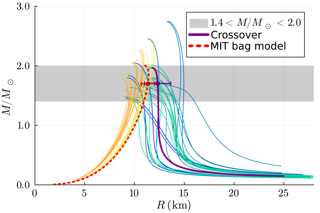
Figure 2: $M$-$R$ curves for NSs (solid) and QSs (dotted). The gray band indicates the mass region favored by current NS observations. At $M=1.7\,M_{\odot}$, the red (QS) and the purple (NS) bars represent the $1\sigma$ width in $R$ estimated from EoS samples.

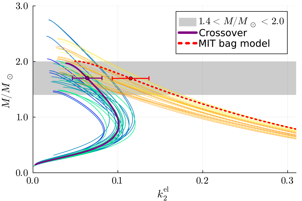
Figure 3: $M$-$k^{\mathrm{el}}_{2}$ curves for NSs (solid) and QSs (dotted). At $M=1.7\,M_{\odot}$, the red (QS) and the purple (NS) bars represent the $1\sigma$ width in $k^{\mathrm{el}}_{2}$ in the same way as Fig. 2.

Magnetic-type Love number:

Following previous studies [48, 50, 63, 64], we assume an irrotational fluid that allows for internal motions induced by the gravitomagnetic interaction with the tidal field, while the tidal field varies slowly and the fluid remains approximately in hydrostatic equilibrium. Even if we calculate $k^{\mathrm{mag}}_{2}$ under the constraint of strict hydrostatic equilibrium following Refs. [49], our conclusion that QSs and NSs are clearly separated in terms of $k^{\mathrm{mag}}_{2}$ is qualitatively unchanged.

As shown in Fig. 4, the curves for QSs and NSs do not intersect in the $M$-$k^{\mathrm{mag}}_{2}$ plane. Therefore, it is possible to distinguish massive QSs from NSs if $k^{\mathrm{mag}}_{2}$ can be determined observationally. For the experimental confirmation of the QS, we do not have to measure $k^{\mathrm{mag}}_{2}$ precisely, but a lower limit of $|k^{\mathrm{mag}}_{2}|$ would be sufficient. Within the range of typical NS EoSs, we find that $|k^{\mathrm{mag}}_{2}|\lesssim 0.0033$ for the high-mass range, $1.4\,M_{\odot}\lesssim M\lesssim 2.0\,M_{\odot}$. Therefore, it is unlikely that the compact object with $|k^{\mathrm{mag}}_{2}|\gtrsim 0.0033$ is the NS. In view of the width in Fig. 4, it would be an undoubted smoking gun if $|k^{\mathrm{mag}}_{2}|\approx 0.004$ is confirmed with a significant confidence level.

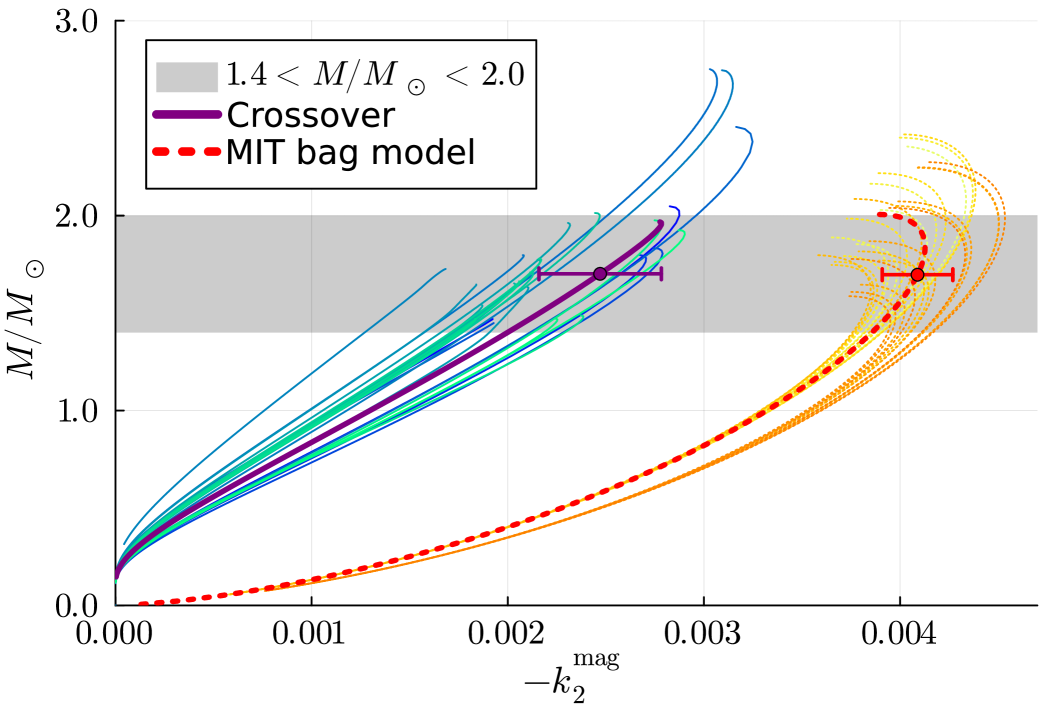
Figure 4: $M$-$k^{\mathrm{mag}}_{2}$ curves for NSs (solid) and QSs (dotted). The horizontal axis shows (irrotational) $-k^{\mathrm{mag}}_{2}$. At $M=1.7\,M_{\odot}$, the red (QS) and the purple (NS) bars represent the $1\sigma$ width in $-k^{\mathrm{mag}}_{2}$ in the same way as Figs. 2 and 3.

Discussions:

So far, we point out that, if QSs and NSs have similar values of $\{M,\,R\}$ in the high-mass region ($M\gtrsim 1.4\,M_{\odot}$), their $\{M,\,k^{\mathrm{el}}_{2}\}$ are also similar. Therefore, even if the precision to measure $k^{\mathrm{el}}_{2}$ in future observations improves significantly, it will still be a difficult challenge to make a conclusive statement of whether the observed object is the QS or the NS based on the $M$-$R$ or $M$-$k^{\mathrm{el}}_{2}$ relation. In contrast, once the information about $M$-$k^{\mathrm{mag}}_{2}$ is available, the comparison between QSs and NSs exhibits clear separation. Thus, $k^{\mathrm{mag}}_{2}$ is a promising physical observable for the QS candidate hunting.

From observational perspectives, we note that it is still under discussion how to measure $k^{\mathrm{mag}}_{2}$ precisely. According to Ref. [65], $k^{\mathrm{mag}}_{2}$ could be detectable with third-generation GW detectors [66, 67], but the proposed test relies on an approximate universal relation between $k^{\mathrm{mag}}_{2}$ and $k^{\mathrm{el}}_{2}$ [51, 68, 69]. As mentioned above, in practice, such a procedure loses independent information about $k^{\mathrm{mag}}_{2}$ in the waveform. Thus, the machinery argued in Ref. [65] is not of practical use to determine $k^{\mathrm{mag}}_{2}$ and $k^{\mathrm{el}}_{2}$ as independent parameters.

The method to measure $\{M,\,k^{\mathrm{el}}_{2},\,k^{\mathrm{mag}}_{2}\}$ independently has not been established yet, while independent measurement of $\{M,\,R,\,k^{\mathrm{el}}_{2}\}$ would be far more difficult, which should involve observation of electromagnetic and gravitational waves simultaneously from the common compact star. The potential advantage in our proposal is that, unlike $\{M,\,R,\,k^{\mathrm{el}}_{2}\}$, we do not have to require simultaneous and different measurements for $\{M,\,k^{\mathrm{el}}_{2},\,k^{\mathrm{mag}}_{2}\}$, because the necessary information is encoded in a single GW observation.

Here, let us assess a prospect to differentiate between QSs and NSs using GW signals. In principle, we can constrain $k^{\mathrm{mag}}_{2}$ from GW observations, if the waveform is identified at arbitrary precision. In the post-Newtonian (PN) expansion of the gravitational waveform, $k^{\mathrm{mag}}_{2}$ first contributes at 6PN order, whereas $k^{\mathrm{el}}_{2}$ first contributes at 5PN order. For waveform modeling, we parameterize the binary components by the masses $M_{i}$, the electric-type tidal deformability $\Lambda_{i}$, and the magnetic-type tidal parameter $\Sigma_{i}$, where $\Lambda$ and $\Sigma$ are related to $k^{\mathrm{el}}_{2}$ and $k^{\mathrm{mag}}_{2}$, respectively, through the compactness. To access $k^{\mathrm{mag}}_{2}$, we must discriminate a QS–QS or QS–NS system from an NS–NS system in six-dimensional parameter space; $(M_{1},\,\Lambda_{1},\,\Sigma_{1})$ and $(M_{2},\,\Lambda_{2},\,\Sigma_{2})$. If the masses are first fixed, parameter space reduces to four dimensions, i.e., space spanned by $(\Lambda_{1},\,\Sigma_{1})$ and $(\Lambda_{2},\,\Sigma_{2})$.

Based on the method explicated in Ref. [70], we can estimate the minimally required signal-to-noise ratio (SNR) to distinguish between two different waveforms, $h_{1}(f)$ and $h_{2}(f)$. With the power spectral density (PSD) denoted by $S_{n}(f)$ (which depends on the detector design), the noise-weighted inner product is defined by

$$\langle h_{1}|h_{2}\rangle=4\,\real\int_{f_{\mathrm{min}}}^{f_{\mathrm{max}}}\frac{h_{1}(f)h_{2}^{*}(f)}{S_{n}(f)}\,df\,.$$ (3)

Using this inner product, the overlap, $F$, maximized with respect to the coalescence time $t_{c}$ and the coalescence phase $\phi_{c}$ is calculated as

$$F(h_{1},h_{2})=\underset{t_{c},\phi_{c}}{\max}\frac{\langle h_{1}|h_{2}\rangle}{\sqrt{\langle h_{1}|h_{1}\rangle}\sqrt{\langle h_{2}|h_{2}\rangle}}$$ (4)

To distinguish these two waveforms in $k$-dimensional parameter space [where $k=6$ for $(M_{i},\,\Lambda_{i},\,\Sigma_{i})$ and $k=4$ for $(\Lambda_{i},\,\Sigma_{i})$], the following condition should be satisfied:

$$2\rho^{2}[1-F(h_{1},h_{2})]\geq\chi^{2}_{k}(1-p)\,,$$ (5)

where $\rho$ is the SNR of our interest, and $\chi_{k}^{2}(1-p)$ is the value of the $\chi$-squared distribution at cumulative probability $1-p$. For a typical case, we compute $h_{1}=h_{\mathrm{BNS}}(f)$ from the Crossover EoS and $h_{2}=h_{\mathrm{BQS}}(f)$ from the MIT bag model EoS. In both cases, the component masses are fixed to $M_{1}=M_{2}=1.4\ M_{\odot}$, with which $(\Lambda_{i},\,\Sigma_{i})$ are uniquely derived from the EoSs. We calculate the waveforms with TaylorF2 ($3.5$PN) plus multipolar tidal terms with ($\Lambda_{i},\,\Sigma_{i}$); see Ref. [71] for details. We use the noise PSD, $S_{n}(f)$, from the ET-B design sensitivity curve [67]. We summarize the required SNR values below:

$k$	$\rho$ $(68\%)$	$\rho$ $(90\%)$
$4$	63.9	82.2
$6$	78.0	96.2

These required $\rho$ values indicate that, to distinguish the binary QS merger from the binary NS merger using GW signals, one needs either a lower detector noise $S_{n}(f)$ or closer/louder events. For scale reference, the combined SNR of GW170817 was $32.4$ ($18.8$, $26.4$, and $2.0$ in LIGO–Hanford, LIGO–Livingston, and Virgo, respectively) [37], so our threshold $\rho\geq 63.9$ is about twice as large.

Summary:

We found that $k^{\mathrm{mag}}_{2}$ takes substantially different values for QSs and NSs even if their masses and radii are almost degenerate. Our findings should extend the frontier of the QS search toward higher mass regions and thus enhance the opportunity to identify the candidates in the near future. We pointed out that the most notable advantage of considering $k^{\mathrm{mag}}_{2}$ is that we do not have to make an independent measurement, but a single GW signal conveys all information. For a test of measurability, we exploited GW signals encoding $k^{\mathrm{el}}_{2}$ and $k^{\mathrm{mag}}_{2}$, and estimated the SNR necessary for distinguishing between two scenarios of the binary QS merger and the binary NS merger. From our results, we can conclude that the idea of differentiating QS candidates among seemingly NS-like objects with $k^{\mathrm{mag}}_{2}$ is promising. The potential of magnetic-type Love number would deserve further investigations along the lines of more realistic simulations in the future.

I Acknowledgments

The authors thank Toru Kojo and Shuhei Minato for useful discussions. They are grateful to Hajime Sotani for a warmful hospitality at Kochi University where a part of this work was completed. This work was supported by Japan Society for the Promotion of Science (JSPS) KAKENHI Grant No. 22H01216 (K.F.) and FoPM, WINGS Program, The University of Tokyo (T.U.).

References

- Bodmer [1971] A. R. Bodmer, Phys. Rev. D 4, 1601 (1971).
- Farhi and Jaffe [1984] E. Farhi and R. L. Jaffe, Phys. Rev. D 30, 2379 (1984).
- Witten [1984] E. Witten, Phys. Rev. D 30, 272 (1984).
- Itoh [1970] N. Itoh, Prog. Theor. Phys. 44, 291 (1970).
- Fechner and Joss [1978] W. B. Fechner and P. C. Joss, Nature 274, 347 (1978).
- Alcock et al. [1986] C. Alcock, E. Farhi, and A. Olinto, Astrophys. J. 310, 261 (1986).
- Haensel et al. [1986] P. Haensel, J. L. Zdunik, and R. Schaeffer, Astron. Astrophys. 160, 121 (1986).
- Bombaci et al. [2004] I. Bombaci, I. Parenti, and I. Vidana, Astrophys. J. 614, 314 (2004), arXiv:astro-ph/0402404 .
- Weber [2005] F. Weber, Prog. Part. Nucl. Phys. 54, 193 (2005), arXiv:astro-ph/0407155 .
- Jaikumar et al. [2006] P. Jaikumar, S. Reddy, and A. W. Steiner, Phys. Rev. Lett. 96, 041101 (2006), arXiv:nucl-th/0507055 .
- Sotani and Harada [2003] H. Sotani and T. Harada, Phys. Rev. D 68, 024019 (2003), arXiv:gr-qc/0307035 .
- Fu et al. [2008] W.-j. Fu, H.-q. Wei, and Y.-x. Liu, Phys. Rev. Lett. 101, 181102 (2008), arXiv:0810.1084 [nucl-th] .
- Watts and Reddy [2007] A. L. Watts and S. Reddy, Mon. Not. Roy. Astron. Soc. 379, L63 (2007), arXiv:astro-ph/0609364 .
- Traversi and Char [2020] S. Traversi and P. Char, Astrophys. J. 905, 9 (2020), arXiv:2007.10239 [nucl-th] .
- Zou et al. [2022] Z.-C. Zou, Y.-F. Huang, and X.-L. Zhang, Universe 8, 442 (2022), arXiv:2207.12053 [astro-ph.HE] .
- Drago et al. [2014] A. Drago, A. Lavagno, and G. Pagliara, Phys. Rev. D 89, 043014 (2014), arXiv:1309.7263 [nucl-th] .
- Li et al. [2016] A. Li, B. Zhang, N. B. Zhang, H. Gao, B. Qi, and T. Liu, Phys. Rev. D 94, 083010 (2016), [Addendum: Phys.Rev.D 102, 029902 (2020)], arXiv:1606.02934 [astro-ph.HE] .
- Holdom et al. [2018] B. Holdom, J. Ren, and C. Zhang, Phys. Rev. Lett. 120, 222001 (2018), arXiv:1707.06610 [hep-ph] .
- Bombaci et al. [2021] I. Bombaci, A. Drago, D. Logoteta, G. Pagliara, and I. Vidaña, Phys. Rev. Lett. 126, 162702 (2021), arXiv:2010.01509 [nucl-th] .
- Doroshenko et al. [2022] V. Doroshenko, V. Suleimanov, G. Pühlhofer, and A. Santangelo, Nature Astronomy 6, 1444 (2022).
- Abbott et al. [2020] R. Abbott et al. (LIGO Scientific, Virgo), Astrophys. J. Lett. 896, L44 (2020), arXiv:2006.12611 [astro-ph.HE] .
- Nagata [2022] K. Nagata, Prog. Part. Nucl. Phys. 127, 103991 (2022), arXiv:2108.12423 [hep-lat] .
- Fujimoto et al. [2024] Y. Fujimoto, K. Fukushima, S. Kamata, and K. Murase, Phys. Rev. D 110, 034035 (2024), arXiv:2401.12688 [nucl-th] .
- Kurkela et al. [2010] A. Kurkela, P. Romatschke, and A. Vuorinen, Phys. Rev. D 81, 105021 (2010), arXiv:0912.1856 [hep-ph] .
- Gorda et al. [2018] T. Gorda, A. Kurkela, P. Romatschke, S. Säppi, and A. Vuorinen, Phys. Rev. Lett. 121, 202701 (2018), arXiv:1807.04120 [hep-ph] .
- Fujimoto et al. [2021] Y. Fujimoto, K. Fukushima, and K. Murase, JHEP 03, 273, arXiv:2101.08156 [nucl-th] .
- Altiparmak et al. [2022] S. Altiparmak, C. Ecker, and L. Rezzolla, Astrophys. J. Lett. 939, L34 (2022), arXiv:2203.14974 [astro-ph.HE] .
- Marczenko et al. [2023] M. Marczenko, L. McLerran, K. Redlich, and C. Sasaki, Phys. Rev. C 107, 025802 (2023), arXiv:2207.13059 [nucl-th] .
- Brandes et al. [2023] L. Brandes, W. Weise, and N. Kaiser, Phys. Rev. D 108, 094014 (2023), arXiv:2306.06218 [nucl-th] .
- Annala et al. [2020] E. Annala, T. Gorda, A. Kurkela, J. Nättilä, and A. Vuorinen, Nature Phys. 16, 907 (2020), arXiv:1903.09121 [astro-ph.HE] .
- Most et al. [2019] E. R. Most, L. J. Papenfort, V. Dexheimer, M. Hanauske, S. Schramm, H. Stöcker, and L. Rezzolla, Phys. Rev. Lett. 122, 061101 (2019), arXiv:1807.03684 [astro-ph.HE] .
- Weih et al. [2020] L. R. Weih, M. Hanauske, and L. Rezzolla, Phys. Rev. Lett. 124, 171103 (2020), arXiv:1912.09340 [gr-qc] .
- Bauswein et al. [2022] A. Bauswein, D. B. Blaschke, and T. Fischer, Effects of a strong phase transition on supernova explosions, compact stars and their mergers, in Astrophysics in the XXI Century with Compact Stars (2022) Chap. Chapter 8, pp. 283–320, arXiv:2203.17188 [nucl-th] .
- Fujimoto et al. [2023] Y. Fujimoto, K. Fukushima, K. Hotokezaka, and K. Kyutoku, Phys. Rev. Lett. 130, 091404 (2023), arXiv:2205.03882 [astro-ph.HE] .
- Fujimoto et al. [2025] Y. Fujimoto, K. Fukushima, K. Hotokezaka, and K. Kyutoku, Phys. Rev. D 111, 063054 (2025), arXiv:2408.10298 [astro-ph.HE] .
- Annala et al. [2018] E. Annala, T. Gorda, A. Kurkela, and A. Vuorinen, Phys. Rev. Lett. 120, 172703 (2018), arXiv:1711.02644 [astro-ph.HE] .
- Abbott et al. [2017] B. P. Abbott et al. (LIGO Scientific, Virgo), Phys. Rev. Lett. 119, 161101 (2017), arXiv:1710.05832 [gr-qc] .
- Hinderer [2008] T. Hinderer, Astrophys. J. 677, 1216 (2008), [Erratum: Astrophys.J. 697, 964 (2009)], arXiv:0711.2420 [astro-ph] .
- Zhou et al. [2018] E.-P. Zhou, X. Zhou, and A. Li, Phys. Rev. D 97, 083015 (2018), arXiv:1711.04312 [astro-ph.HE] .
- Cao et al. [2022] Z. Cao, L.-W. Chen, P.-C. Chu, and Y. Zhou, Phys. Rev. D 106, 083007 (2022), arXiv:2009.00942 [astro-ph.HE] .
- Li et al. [2021] A. Li, Z.-Q. Miao, J.-L. Jiang, S.-P. Tang, and R.-X. Xu, Mon. Not. Roy. Astron. Soc. 506, 5916 (2021), arXiv:2009.12571 [astro-ph.HE] .
- Miao et al. [2021] Z. Miao, J.-L. Jiang, A. Li, and L.-W. Chen, Astrophys. J. Lett. 917, L22 (2021), arXiv:2107.13997 [astro-ph.HE] .
- Miao et al. [2022] Z. Miao, A. Li, and Z.-G. Dai, Mon. Not. Roy. Astron. Soc. 515, 5071 (2022), arXiv:2107.07979 [astro-ph.HE] .
- Miao et al. [2025] Z. Miao, Z. Zhu, and D. Lai, Phys. Rev. Lett. 135, 091402 (2025), arXiv:2411.09013 [astro-ph.HE] .
- Shirke et al. [2025] S. Shirke, R. Maiti, and D. Chatterjee, e-Print (2025), arXiv:2508.02652 [astro-ph.HE] .
- Alford et al. [2005] M. Alford, M. Braby, M. W. Paris, and S. Reddy, Astrophys. J. 629, 969 (2005), arXiv:nucl-th/0411016 .
- Yagi and Yunes [2017] K. Yagi and N. Yunes, Phys. Rept. 681, 1 (2017), arXiv:1608.02582 [gr-qc] .
- Damour and Nagar [2009] T. Damour and A. Nagar, Phys. Rev. D 80, 084035 (2009), arXiv:0906.0096 [gr-qc] .
- Binnington and Poisson [2009] T. Binnington and E. Poisson, Phys. Rev. D 80, 084018 (2009), arXiv:0906.1366 [gr-qc] .
- Landry and Poisson [2015] P. Landry and E. Poisson, Phys. Rev. D 91, 104026 (2015), arXiv:1504.06606 [gr-qc] .
- Yagi [2014] K. Yagi, Phys. Rev. D 89, 043011 (2014), [Erratum: Phys.Rev.D 96, 129904 (2017), Erratum: Phys.Rev.D 97, 129901 (2018)], arXiv:1311.0872 [gr-qc] .
- Postnikov et al. [2010] S. Postnikov, M. Prakash, and J. M. Lattimer, Phys. Rev. D 82, 024016 (2010), arXiv:1004.5098 [astro-ph.SR] .
- Chodos et al. [1974] A. Chodos, R. L. Jaffe, K. Johnson, C. B. Thorn, and V. F. Weisskopf, Phys. Rev. D 9, 3471 (1974).
- DeGrand et al. [1975] T. A. DeGrand, R. L. Jaffe, K. Johnson, and J. E. Kiskis, Phys. Rev. D 12, 2060 (1975).
- Baym et al. [2018] G. Baym, T. Hatsuda, T. Kojo, P. D. Powell, Y. Song, and T. Takatsuka, Rept. Prog. Phys. 81, 056902 (2018), arXiv:1707.04966 [astro-ph.HE] .
- Fraga et al. [2014] E. S. Fraga, A. Kurkela, and A. Vuorinen, Astrophys. J. Lett. 781, L25 (2014), arXiv:1311.5154 [nucl-th] .
- Buballa [2005] M. Buballa, Phys. Rept. 407, 205 (2005), arXiv:hep-ph/0402234 .
- Vogl and Weise [1991] U. Vogl and W. Weise, Prog. Part. Nucl. Phys. 27, 195 (1991).
- Klevansky [1992] S. P. Klevansky, Rev. Mod. Phys. 64, 649 (1992).
- Hatsuda and Kunihiro [1994] T. Hatsuda and T. Kunihiro, Phys. Rept. 247, 221 (1994), arXiv:hep-ph/9401310 .
- Rehberg et al. [1996] P. Rehberg, S. P. Klevansky, and J. Hufner, Phys. Rev. C 53, 410 (1996), arXiv:hep-ph/9506436 .
- Read et al. [2009] J. S. Read, B. D. Lackey, B. J. Owen, and J. L. Friedman, Phys. Rev. D 79, 124032 (2009), arXiv:0812.2163 [astro-ph] .
- Favata [2006] M. Favata, Phys. Rev. D 73, 104005 (2006), arXiv:astro-ph/0510668 .
- Shapiro [1996] S. L. Shapiro, Phys. Rev. Lett. 77, 4487 (1996).
- Jiménez Forteza et al. [2018] X. Jiménez Forteza, T. Abdelsalhin, P. Pani, and L. Gualtieri, Phys. Rev. D 98, 124014 (2018), arXiv:1807.08016 [gr-qc] .
- Punturo et al. [2010] M. Punturo et al., Class. Quant. Grav. 27, 084007 (2010).
- Hild et al. [2011] S. Hild et al., Class. Quant. Grav. 28, 094013 (2011), arXiv:1012.0908 [gr-qc] .
- Gagnon-Bischoff et al. [2018] J. Gagnon-Bischoff, S. R. Green, P. Landry, and N. Ortiz, Phys. Rev. D 97, 064042 (2018), arXiv:1711.05694 [gr-qc] .
- Pani et al. [2018] P. Pani, L. Gualtieri, T. Abdelsalhin, and X. Jiménez-Forteza, Phys. Rev. D 98, 124023 (2018), arXiv:1810.01094 [gr-qc] .
- Lindblom et al. [2008] L. Lindblom, B. J. Owen, and D. A. Brown, Phys. Rev. D 78, 124020 (2008), arXiv:0809.3844 [gr-qc] .
- Henry et al. [2020] Q. Henry, G. Faye, and L. Blanchet, Phys. Rev. D 102, 044033 (2020), [Erratum: Phys.Rev.D 108, 089901 (2023), Erratum: Phys.Rev.D 111, 029901 (2025)], arXiv:2005.13367 [gr-qc] .