Diffusion Index Forecast with Tensor Data

Abstract

In this paper, we consider diffusion index forecast with both tensor and non-tensor predictors, where the tensor structure is preserved with a Canonical Polyadic (CP) tensor factor model. When the number of non-tensor predictors is small, we study the asymptotic properties of the least-squared estimator in this tensor factor-augmented regression, allowing for factors with different strengths. We derive an analytical formula for prediction intervals that accounts for the estimation uncertainty of the latent factors. In addition, we propose a novel thresholding estimator for the high-dimensional covariance matrix that is robust to cross-sectional dependence. When the number of non-tensor predictors exceeds or diverges with the sample size, we introduce a multi-source factor-augmented sparse regression model and establish the consistency of the corresponding penalized estimator. Simulation studies validate our theoretical results and an empirical application to US trade flows demonstrates the advantages of our approach over other popular methods in the literature.

JEL Classifications: C13, C32, C55

Keywords: Canonical Polyadic (CP) Decompositions, Diffusion Index, Factor models, Forecast, High-dimensional, LASSO, Tensor data.

1 Introduction

Since the seminal work of Stock and Watson, (2002) and Bai and Ng, (2006), diffusion index forecast has been widely adopted by government agencies, policy institutes, and academic researchers around the world (see, e.g., Ludvigson and Ng, (2007), Ludvigson and Ng, (2009), Jurado et al., (2015)). The classical diffusion index model predicts the target variable as a linear combination of factors extracted from a large panel of time series data, as well as other important predictors. Its strength lies in the ability to significantly reduce the dimensionality of the predictor space by summarizing it into a small number of factors, enabling effective use of large datasets while keeping the size of the forecasting model small.

However, as the availability and complexity of economic data have expanded, new challenges have emerged for forecasting models. In particular, multidimensional data, panel data with more than two dimensions, have attracted increasing attention in economics due to their ability to capture richer and more intricate relationships. For example, consider predicting U.S. import/export volumes with China using monthly time series data. While the traditional gravity model focuses on bilateral trade flows, it may overlook the influence of trade patterns between the U.S., China, and other countries due to substitution effects. Such data can be structured as a three-dimensional tensor, where the observed time series $\mathcal{X}_{t}$ is of dimension $N\times N$ for each period $t$, with $N$ denoting the number of countries in the dataset. This type of multidimensional structure poses challenges to classical diffusion index forecasting, which is based on vector factor models.

A natural approach to tackling this challenge is to flatten or vectorize the tensor time series (see, e.g., Ludvigson and Ng, (2007)) to fit within the framework of vector factor models. However, this process changes the original data structure, potentially diminishing the interpretability of how information from different dimensions interacts. Furthermore, vectorizing tensors often leads to a significant increase in the number of parameters to estimate, which can result in high computational costs.

In this paper, we consider diffusion index forecast with tensor and non-tensor predictors, where the tensor structure is preserved with a Canonical Polyadic (CP) tensor factor model. Common factors are extracted from tensor data using the contemporary covariance-based iterative simultaneous orthogonalization (CC-ISO) procedure proposed in Chen et al., 2024a . When the number of potential non-tensor predictors is small, we estimate the diffusion index model with ordinary least square (OLS) and establish the consistency and asymptotic normality of the estimator. Unlike Bai and Ng, (2006), we allow factors to exhibit different strengths. The convergence rate of the conditional mean prediction for the target variable depends on both the strength of the weakest factor and the sample size. To conduct valid inferences, we propose a thresholding-based covariance matrix estimator that is robust to cross-sectional correlation in the idiosyncratic component and demonstrate its consistency.

When the number of potential non-tensor predictors is large, potentially comparable to or exceeding the sample size, we propose a two-step penalized regression approach, applying least absolute shrinkage and selection operator (LASSO) to select important non-tensor predictors. The combination of factor models and sparse regression has been explored in the literature. In a panel data context, Fan et al., (2024) consider the factor augmented sparse linear regression model, which includes the vector latent factor model and sparse regression as special cases. Chen et al., 2024b extend this framework to matrix-variate data and propose two new algorithms for estimation. However, both papers focus on a single type of predictor, either panel or matrix data. In economic forecasting, researchers often have access to mixed types of data. Consider the trade example again. While trade flows among various countries provide valuable information for predicting U.S. import/export volumes, other economic variables such as GDP, unemployment rates, exchange rates, and interest rates also play a critical role. These different types of data may reflect distinct sources of predictability. The tensor data on trade flows captures global factors while macroeconomic variables act as proxies for local predictability. Our model offers a novel framework for integrating these diverse data sources to improve forecast accuracy.

Our work also relates to several recent developments in econometrics. Within tensor and matrix factor models, recent contributions include Chen and Fan, (2023),Chen et al., 2024a ,Babii et al., (2025), Beyhum and Gautier, (2022), among many others. Our framework differs by focusing on diffusion-index forecasting and integrating both tensor and non-tensor predictors within a unified structure. From the perspective of factor-augmented regressions, classical results often find factor estimation to be first-order neutral for OLS inference (Stock and Watson,, 2002, Bai and Ng,, 2006 and Cai et al.,, 2025), though it can matter in some important cases (Gonçalves and Perron,, 2014). We also contribute to the growing literature on high-dimensional covariance estimation (Bickel and Levina,, 2008,Rothman et al.,, 2009,Fan et al.,, 2013) and on LASSO methods for dependent data (Kock and Callot,, 2015, Medeiros and Mendes,, 2016, Chernozhukov et al.,, 2021, Babii et al.,, 2022, Babii et al.,, 2024 and Beyhum,, 2024). Finally, our empirical application on forecasting international trade follows the standard macro-forecasting tradition, where autoregressive (AR), vector autoregressive (VAR), and diffusion-index models (Stock and Watson,, 2002) as common benchmarks for evaluating forecast performance.

The rest of the paper is organized as follows. In Section 2, we introduce the diffusion index forecast based on the CP tensor factor model and develop the estimator when the number of non-tensor predictors is small. Section 3 derives the inferential theories for the diffusion index model and proposes a robust covariance matrix estimator. Section 4 introduces multi-source factor-augmented sparse regression to combine information from different sources and discusses the consistency of the proposed estimator. In Section 5, a simulation study is conducted to assess the reliability of the low- and high-dimensional estimators in finite samples. In Section 6, an empirical example on US export/import forecasting highlights the merits of our approach in comparison with some popular methods in the literature. All mathematical proofs and additional simulation results are contained in the Appendix.

1.1 Notation and Preliminaries

In this subsection, we introduce essential notations and basic tensor operations. For an in-depth review, readers may refer to Kolda and Bader, (2009).

Let $\|x\|_{q}=(x_{1}^{q}+...+x_{p}^{q})^{1/q}$, $q\geq 1$, for any vector $x=(x_{1},...,x_{p})^{\top}$. In particular, $\|x\|_{\infty}=\max_{1\leq j\leq p}|x_{j}|$. We employ the following matrix norms: matrix spectral norm $\|M\|_{2}=\underset{\|x\|_{2}=1,\|y\|_{2}=1}{\max}|x^{\top}My|=\sigma_{1}(M)$, where $\sigma_{1}(M)$ is the largest singular value of $M$; max entry norm: $\left\|M\right\|_{\max}=\max_{1\leq i\leq p,1\leq j\leq q}|M_{ij}|$ for $M\in\mathbb{R}^{p\times q}$, where $M_{ij}$ denotes the $(i,j)$ entry of $M$. For two sequences of real numbers $\{a_{n}\}$ and $\{b_{n}\}$, we write $a_{n}\lesssim b_{n}$ (respectively, $a_{n}\gtrsim b_{n}$) if there exists a constant $C$ such that $|a_{n}|\leq C|b_{n}|$ (respectively, $|a_{n}|\geq C|b_{n}|$) holds for all sufficiently large $n$, and $a_{n}\asymp b_{n}$ if both $a_{n}\lesssim b_{n}$ and $a_{n}\gtrsim b_{n}$ hold.

Consider two tensors ${\cal A}\in\mathbb{R}^{d_{1}\times d_{2}\times\cdots\times d_{K}},{\cal B}\in\mathbb{R}^{p_{1}\times p_{2}\times\cdots\times p_{N}}$. The outer product $\otimes$ is defined as ${\cal A}\otimes{\cal B}\in\mathbb{R}^{d_{1}\times\cdots\times d_{K}\times p_{1}\times\cdots\times p_{N}}$, where

$$({\cal A}\otimes{\cal B})_{i_{1},...,i_{K},j_{1},...,j_{N}}=({\cal A})_{i_{1},...,i_{K}}({\cal B})_{j_{1},...,j_{N}}.$$

The mode-$k$ product of ${\cal A}\in\mathbb{R}^{d_{1}\times d_{2}\times\cdots\times d_{K}}$ with a matrix $U\in\mathbb{R}^{d_{k}\times r_{k}}$ is an order $K$-tensor of size $d_{1}\times\cdots\times d_{k-1}\times r_{k}\times d_{k+1}\times\cdots\times d_{K}$, denoted as ${\cal A}\times_{k}U^{\top}$, where

$$({\cal A}\times_{k}U)_{i_{1},...,i_{k-1},j,i_{k+1},...,i_{K}}=\sum_{i_{k}=1}^{d_{k}}{\cal A}_{i_{1},i_{2},...,i_{K}}U_{j,i_{k}}.$$

Given ${\cal A}\in\mathbb{R}^{d_{1}\times d_{2}\times\cdots\times d_{K}}$ and a sequence of $\{U_{k}\}_{k=1}^{K}$, where $U_{k}\in\mathbb{R}^{d_{k}\times r_{k}}$, the notation ${\cal A}\times_{k=1}^{K}U_{k}^{\top}$ denotes a sequence of mode-$k$ product:

$${\cal A}\times_{k=1}^{K}U_{k}^{\top}={\cal A}\times_{1}U_{1}^{\top}\times_{2}U_{2}^{\top}\times\cdots\times_{K}U_{K}^{\top}\in\mathbb{R}^{r_{1}\times r_{2}\times\cdots\times r_{K}}.$$

The Khatri-Rao (or column-wise Kronecker) product of two matrices $A=(a_{1},a_{2},\cdots,a_{r})$ and $B=(b_{1},b_{2},\cdots,b_{r})$ is defined as $A*B=(a_{1}\odot b_{1},\cdots,a_{r}\odot b_{r})$, where $\odot$ denotes the Kronecker product. Denote $d=d_{1}\times d_{2}\times\cdots\times d_{K}$, $d_{\min}=\min_{k\leq K}d_{k}$ and $d_{\max}=\max_{k\leq K}d_{k}$.

2 Model and Estimation

Assume that a decision maker is interested in predicting some univariate series $y_{t+h}$, conditional on $I_{t}$, the information available at time $t$, which consists of a tensor-variate predictor ${\cal X}_{t}\in\mathbb{R}^{d_{1}\times d_{2}\times\cdots\times d_{K}}$ and a set of other observable variables $w_{t}\in\mathbb{R}^{p}$, such as lags of $y_{t}$. We consider a diffusion index forecast model as

$$y_{t+h}=\beta_{0}^{\top}w_{t}+\beta_{1}^{\top}f_{t}+\epsilon_{t+h},\quad t=1,...,T,$$ (1)

where $h\geq 0$ is the lead time between information available and the target variable. The vector $f_{t}=(f_{1t},\ldots,f_{rt})^{\top}$ consists of $r$ latent factors extracted from the observed tensor data ${\cal X}_{t}$. Specifically, we model ${\cal X}_{t}$ as a tensor factor model with a CP low-rank structure:

$${\cal X}_{t} =\sum_{i=1}^{r}f_{it}(\widetilde{a}_{i1}\otimes\widetilde{a}_{i2}\otimes\cdots\otimes\widetilde{a}_{iK})+{\cal E}_{t}=\sum_{i=1}^{r}s_{i}f_{it}(a_{i1}\otimes a_{i2}\otimes\cdots\otimes a_{iK})+{\cal E}_{t},$$ (2)

where $r$ denotes the fixed number of factors and $\widetilde{a}_{ik}$ denotes the $d_{k}$-dimensional loading vector, which needs not to be orthogonal. Without loss of generality and to ensure identifiability, we assume that $\mathbb{E}f_{it}^{2}=1$ and normalize the factor loadings $\widetilde{a}_{ik}$ so that $\|a_{ik}\|_{2}=1$, for all $1\leq i\leq r$ and $1\leq k\leq K$. Consequently, all factor strengths are captured by $s_{i}$. In the strong factor model case, $\|\widetilde{a}_{ik}\|_{2}\asymp\sqrt{d_{k}}$, which implies that $s_{i}\asymp\sqrt{d_{1}d_{2}\cdots d_{K}}$. The construction of $s_{i}$ is a matter of parametrization, which ensures the order of the estimated factor $\widehat{f}_{t}$ to be $O_{p}(1)$ by convention. The noise tensor $\mathcal{E}_{t}$ is assumed to be uncorrelated with the latent factors but may exhibit weak correlations across different dimensions. Unlike classical vector factor models, which suffer from rotation ambiguity, the CP tensor factors are uniquely identified up to sign changes (Kruskal,, 1977, 1989; Sidiropoulos and Bro,, 2000). Throughout this paper, we assume the sign of factors is known without loss of generality.

To construct forecasts for $y_{T+h}$, the CP factor model (2) needs to be estimated first. We adopt the CC-ISO method proposed by Chen et al., 2024a in our context. Specifically, we estimate $f_{t}$ via the following algorithm.

Step 1. Obtain the initial value $\widehat{A}_{k}^{(0)}=(\widehat{a}_{1k}^{(0)},\ldots,\widehat{a}_{rk}^{(0)})\in\mathbb{R}^{d_{k}\times r}$ via randomized composite PCA (Chen et al., 2024a, ) or tensor PCA (Babii et al.,, 2023) and compute $\widehat{B}_{k}^{(0)}=\widehat{A}_{k}^{(0)}(\widehat{A}_{k}^{(0)\top}\widehat{A}_{k}^{(0)})^{-1}=(\widehat{b}_{1k}^{(0)},...,\widehat{b}_{rk}^{(0)})$, where $1\leq k\leq K$.

Step 2. Given the previous estimates $\widehat{a}_{ik}^{(m-1)}$, where $m$ is the iteration number, calculate

$${\cal Z}_{t,ik}^{(m)}={\cal X}_{t}\times_{1}\widehat{b}_{i1}^{(m)\top}\times_{2}\cdots\times_{k-1}\widehat{b}_{i,k-1}^{(m)\top}\times_{k+1}\widehat{b}_{i,k+1}^{(m-1)\top}\times_{k+2}\cdots\times_{K}\widehat{b}_{iK}^{(m-1)\top},$$

for $t=1,\cdots,T$. Then the updated loading vectors $\widehat{a}_{ik}^{(m)}$ are obtained as the top eigenvector of the contemporary covariance $\widehat{\Sigma}({\cal Z}_{1:T,ik}^{(m)})=\frac{1}{T}\sum_{t=1}^{T}{\cal Z}_{t,ik}^{(m)}{\cal Z}_{t,ik}^{(m)\top}$, where $1\leq i\leq r$ and $1\leq k\leq K$.

Step 3. Update $\widehat{B}_{k}^{(m)}=\widehat{A}_{k}^{(m)}(\widehat{A}_{k}^{(m)\top}\widehat{A}_{k}^{(m)})^{-1}=(\widehat{b}_{1k}^{(m)},...,\widehat{b}_{rk}^{(m)})$ with $\widehat{A}_{k}^{(m)}=(\widehat{a}_{1k}^{(m)},\ldots,\widehat{a}_{rk}^{(m)})$.

Step 4. Repeat Steps 2 and 3 until the maximum number of iterations $M$ is reached or $\max_{1\leq i\leq r}\max_{1\leq k\leq K}\|\widehat{a}_{ik}^{(m)}\widehat{a}_{ik}^{(m)\top}-\widehat{a}_{ik}^{(m-1)}\widehat{a}_{ik}^{(m-1)\top}\|_{2}\leq\epsilon$, where the default accuracy is set to $\epsilon=10^{-5}$.

Step 5. Obtain the estimated signal as $\widehat{s}_{i}=\sqrt{\frac{\sum_{t=1}^{T}\left({\cal X}_{t}\times_{k=1}^{K}\widehat{b}_{ik}^{\top}\right)^{2}}{T}}$ and the estimated factors as $\widehat{f}_{it}=\widehat{s}_{i}^{-1}\left({\cal X}_{t}\times_{k=1}^{K}\widehat{b}_{ik}^{\top}\right)$, for $i=1,\cdots,r$ and $t=1,\cdots,T$.

The estimated factors, $\widehat{f}_{t}$, along with $w_{t}$, are then used to estimate the coefficients in Equation (1). When the dimension of the non-tensor predictors $w_{t}$ is small, we estimate (1) with OLS and the forecast for $y_{T+h}$ is obtained as

$$\widehat{y}_{T+h}=\widehat{\beta}_{0}^{\top}w_{T}+\widehat{\beta}_{1}^{\top}\widehat{f}_{T},$$

where $\widehat{\beta}_{0}^{\top}$ and $\widehat{\beta}_{1}^{\top}$ are OLS estimates.

The above forecast procedure assumes that the rank of ${\cal X}_{t}$ is known. However, we need to estimate it in practice. We adopt the contemporary covariance-based unfolded eigenvalue ratio estimator considered in Chen et al., 2024a . Other estimators, such as the inner-product-based eigenvalue ratio estimator and autocovariance-based eigen ratio estimator, work as well. More details can be found in Han et al., (2024) and Chen et al., 2024a .

Remark 2.1.

If $y_{t}$ in (1) is a vector of $d$ series and $f_{t}$ is a vector of $r$ univariate factors obtained from ${\cal X}$ via (2), a tensor CP factor-augmented vector autoregressions (TFAVAR) of order $q$ can be constructed as

$$y_{t+1}=\sum_{k=0}^{q}\alpha_{11,k}y_{t-k}+\sum_{k=0}^{q}\alpha_{12,k}f_{t-k}+\epsilon_{1t+1},$$

$$f_{t+1}=\sum_{k=0}^{q}\alpha_{21,k}y_{t-k}+\sum_{k=0}^{q}\alpha_{22,k}f_{t-k}+\epsilon_{2t+1},$$

where $\alpha_{11,k}$, $\alpha_{12,k}$, $\alpha_{21,k}$ and $\alpha_{22,k}$ are model parameters. The inference can be conducted following Bai and Ng, (2006). To stay focused, we only consider the diffusion index forecast and leave TFAVAR for future research.

3 Asymptotic properties

In this section, we consider the asymptotic properties of our estimation when the number of non-tensor predictors is relatively small ($p\ll T$) and thus no regularization is required. Chen et al., 2024a propose the CC-ISO method and focus on the estimation and inference of loadings while the asymptotic properties of latent factors are unknown. Hence, we first fill in the gap by presenting the consistency and asymptotic normality of the estimated latent factors in Section 3.1. Then we derive the inferential theories for the diffusion index model in Section 3.2. Section 3.3 introduces a robust covariance matrix estimator of the factor process for conducting inference on the conditional mean forecasts.

3.1 Estimation of Factors

We start with some assumptions that are necessary for our theoretical development.

Assumption 3.1.

Denote $e_{t}=\mbox{vec}({\cal E}_{t})\in\mathbb{R}^{d}$ where $d=\prod_{k=1}^{K}d_{k}$ and $f_{t}=(f_{1t},...,f_{rt})^{\top}$,

1. For any $v\in\mathbb{R}^{r}$ with $\|v\|_{2}=1$ and any $u\in\mathbb{R}^{d}$ with $\|u\|_{2}=1$,

   $$\max_{t}\mathbb{P}\left(|u^{\top}e_{t}|\geq x\right)\leq c_{1}\exp(-c_{2}x^{\nu_{1}}),$$ (3)

   $$\max_{t}\mathbb{P}\left(\left|v^{\top}f_{t}\right|\geq x\right)\leq c_{1}\exp\left(-c_{2}x^{\nu_{2}}\right),$$ (4)

   for some constants $c_{1},c_{2},\nu_{1},\nu_{2}>0$.

2. Assume $\left(f_{t},e_{t}\right)$ is stationary and $\alpha$-mixing. The mixing coefficient satisfies

   $$\alpha(m)\leq\exp\left(-c_{0}m^{\gamma}\right)$$ (5)

   for some constants $c_{0}>0$ and $\gamma\geq 0$, where

   $$\alpha(m)=\sup_{t}\Big\{ \Big|\mathbb{P}(A\cap B)-\mathbb{P}(A)\mathbb{P}(B)\Big|:$$

   $$A\in\sigma\left(\left(f_{s},e_{s}\right),s\leq t\right),B\in\sigma\left(\left(f_{s},e_{s}\right),1\leq i\leq r,s\geq t+m\right)\Big\}.$$

3. Denote $\Sigma_{e}=\mathbb{E}(e_{t}e_{t}^{\top})$ and $\Sigma_{f}=\mathbb{E}(f_{t}f_{t}^{\top})$. There exists a constant $C_{0}>0$ such that $\|\Sigma_{e}\|_{2}\leq C_{0}$ and $C_{0}^{-1}\leq\lambda_{r}(\Sigma_{f})\leq\cdots\leq\lambda_{1}(\Sigma_{f})\leq C_{0}$, where $\lambda_{i}(\Sigma_{f})$ denotes the $i^{th}$ largest eigenvalue of $\Sigma_{f}$.

4. The factor process $f_{t}$ is independent of the errors $e_{t}$.

Assumption 3.2.

Denote $d_{\max}=\max_{1\leq k\leq K}d_{k}$, $\frac{1}{\eta_{1}}=\frac{2}{\nu_{1}}+\frac{1}{\gamma}$, $\frac{1}{\eta_{2}}=\frac{\nu_{1}+\nu_{2}}{\nu_{1}\nu_{2}}+\frac{1}{\gamma}$ and $\frac{1}{\eta_{3}}=\frac{2}{\nu_{2}}+\frac{1}{\gamma}$. Assume $\min\{\frac{1}{\eta_{1}},\frac{1}{\eta_{2}},\frac{1}{\eta_{3}}\}>1$. The signal components satisfy $s_{i}^{2}\asymp d^{\alpha_{i}}$ for some $0<\alpha_{r}\leq\alpha_{r-1}\leq\cdots\leq\alpha_{1}\leq 1$ such that:

$$\sqrt{\frac{d_{\max}}{d^{\alpha_{r}}T}}+\frac{d_{\max}^{1/\eta_{1}}}{d^{\alpha_{r}}T}+\frac{d_{\max}^{1/\eta_{2}}}{d^{\alpha_{r}/2}T}+\frac{1}{\sqrt{T}}=O(1).$$

Assumption 3.1 (i) assumes that the tails of the error and factor processes exhibit exponential decay, which includes a sub-Gaussian distribution as an important example. This assumption could be extended to account for polynomial-type tails with bounded moment conditions. Unlike Lam and Yao, (2012), Han et al., (2024) and Chen et al., 2024a , Assumption 3.1(ii) and (iii) allow both weak cross-sectional and serial correlations in the error term. Assumption 3.1(ii) assumes the $\alpha$-mixing property on the factor process, a standard assumption assumed in the tensor factor literature to capture temporal dependence (e.g., Chen and Fan,, 2023 and Han et al.,, 2024). We acknowledge that the $\alpha$-mixing condition might not be flexible enough to accommodate certain time series models (Andrews,, 1984). Nevertheless, to maintain focus on the essential theoretical developments and ensure analytical tractability, we adopt the $\alpha$-mixing framework in the main analysis. Possible relaxations of this assumption are discussed in Appendix E.

A sufficient condition for Assumption 3.1 is $\max_{j}\sum_{l=1}^{d}|{\mathbb{E}}\left[e_{jt}e_{lt}\right]|<\infty$, which ensures that the aggregate dependence across all pairs of cross-sectional units remains bounded as $d$ increases. This condition is mild and commonly used in large-dimensional factor, panel, and matrix-valued time series models (e.g., Bai,, 2003, Chen and Fan,, 2023). If the cross-sectional dimension has some natural ordering (e.g., spatial or social network data), ${e_{jt}}$ may be assumed to be $\alpha$-mixing in the cross-sectional dimension as well. Namely, for each $t=1,\cdots,T$, ${e_{jt}}$ is $\alpha-$mixing with mixing coefficients $\alpha_{t}(m)$ such that $\sup_{t}\alpha_{t}(m)\leq\alpha(m)$. Then it is straightforward to verify that Assumption 3.1 (iii) holds by the mixing inequality. Alternatively, if we take into account the tensor structure, we can consider an example as in Appendix C, which allows for exponentially decaying error correlation along both tensor modes. If there is no natural ordering for cross-sectional indices, one can follow Chen et al., (2012) by introducing a "distance function" between cross-sectional units to define a weak dependence structure that also satisfies Assumption 3.1 (iii).

Assumption 3.1 (iv) imposes independence between factors and errors, which simplifies the analysis of both the ISO algorithm and the forecast model. A more general assumption allowing for limited dependence, as suggested by Bai, (2003), could also be considered, though it would introduce significantly greater theoretical complexity.

Unlike Bai, (2003) and Fan et al., (2024), Assumption 3.2 allows for varying factor strengths by incorporating a mix of strong and weak factors, with certain conditions on the weakest signal strength, the dimensions of tensor data, and the sample size. Specifically, it ensures that, as $d,T\to\infty$, $\max_{i\leq r,k\leq K}\|\widehat{a}_{ik}\widehat{a}_{ik}^{\top}-a_{ik}a_{ik}^{\top}\|_{2}\to 0$, thereby guaranteeing the consistency of the factor estimation.

Let $\psi_{0}$ denote the estimation error of the warm-start initial estimates for the factor loading vectors. Define $H=\operatorname{diag}(s_{1}\widehat{s}_{1}^{-1},\cdots,s_{r}\widehat{s}_{r}^{-1})$. For the ease of notation, we define

$$\psi=\sqrt{\frac{d_{\max}}{d^{\alpha_{r}}T}}+\frac{d_{\max}^{1/\eta_{1}}}{d^{\alpha_{r}}T}+\frac{d_{\max}^{1/\eta_{2}}}{d^{\alpha_{r}/2}T}+\frac{1}{d^{\alpha_{r}}},$$ (6)

which represents the final estimation error for the factor loading vectors. We first present the performance bounds of $\widehat{f}_{t}$ below.

Theorem 3.1.

Suppose Assumptions 3.1- 3.2 hold. Assume that

$\max_{k\leq K}\|A_{k}^{\top}A_{k}-I_{r}\|_{2}<1$ and $T\leq C\exp\left(d_{\max}\right)$ for some constant $C$. Suppose that the initial estimation error bounds satisfy the condition:

$$C_{1,K}\left(\frac{s_{1}^{2}}{s_{r}^{2}}\right)\psi_{0}^{2K-3}+C_{1,K}\frac{s_{1}}{s_{r}}\left(\sqrt{\frac{\log T}{T}}+\frac{(\log T)^{1/\eta_{3}}}{T}\right)\psi_{0}^{K-2}\leq\rho<1,$$ (7)

where $C_{1,K}$ is some constant depending on $K$ only. Then the estimated tensor factors satisfy

$$\begin{split}&(i)\quad\|\widehat{f}_{t}-Hf_{t}\|_{2}=O_{p}\left(\psi+\frac{1}{d^{\alpha_{r}/2}}\right),\\ &(ii)\quad\|\widehat{f}_{t}-f_{t}\|_{2}=O_{p}\left(\psi+\frac{1}{d^{\alpha_{r}/2}}+\sqrt{\frac{1}{T}}\right).\end{split}$$ (8)

Theorem 3.1 shows that $\widehat{f}_{t}$ is a consistent estimator of the latent factor $f_{t}$. However, the convergence rate of $\widehat{f}_{t}$ to $f_{t}$ may be slower compared to its convergence to $Hf_{t}$. This discrepancy arises due to the non-negligible estimation error associated with the factor signal $s_{i}$. Nevertheless, this does not affect the prediction of $y_{t+h}$, as the impact is absorbed by the coefficient $\beta_{1}$. We will provide further discussion on this point in Section 6. When all factors are strong, i.e., $\alpha_{i}=1$ for all $1\leq i\leq r$, Theorem 3.1 implies the following:

$$\begin{split}&\|\widehat{f}_{t}-Hf_{t}\|_{2}=O_{p}\left(\sqrt{\frac{d_{\max}}{dT}}+\frac{d_{\max}^{1/\eta_{1}}}{dT}+\frac{d_{\max}^{1/\eta_{2}}}{d^{1/2}T}+\sqrt{\frac{1}{d}}\right),\\ &\|\widehat{f}_{t}-f_{t}\|_{2}=O_{p}\left(\sqrt{\frac{d_{\max}}{dT}}+\frac{d_{\max}^{1/\eta_{1}}}{dT}+\frac{d_{\max}^{1/\eta_{2}}}{d^{1/2}T}+\sqrt{\frac{1}{d}}+\sqrt{\frac{1}{T}}\right).\end{split}$$

If we further assume that the error term is serially uncorrelated and follows a sub-Gaussian distribution, then the rates simplify to:

$$\begin{split}\|\widehat{f}_{t}-Hf_{t}\|_{2}&=O_{p}\left(\sqrt{\frac{d_{\max}}{dT}}+\sqrt{\frac{1}{d}}\right),\\ \|\widehat{f}_{t}-f_{t}\|_{2}&=O_{p}\left(\sqrt{\frac{1}{T}}+\sqrt{\frac{1}{d}}\right).\end{split}$$

Remark 3.1.

As $\|a_{ik}\|_{2}^{2}=1$, $\|A_{k}^{\top}A_{k}-I_{r}\|_{2}<1$ is used to measure the correlation among columns of $A_{k}$. If the loadings are orthogonal, this condition is automatically satisfied. If we define the maximum coherence level as $\varrho_{k}=\max_{i\neq j}|a_{ik}a_{jk}|$, one sufficient condition is $(r-1)\varrho_{k}<1$.

Remark 3.2.

The matrix $H$ is introduced to capture the estimation uncertainty of the factor strengths $s_{i}$, $i=1,\cdots,r$. Since the factor strengths must be estimated in order to recover $f_{t}$ (rather than the scaled version $Hf_{t}$), the presence of the $1/\sqrt{T}$ term is inevitable. The use of $H$ effectively removes this source of uncertainty, and the resulting convergence rate with $H$ in Theorem 3.1 is indeed optimal in the time series setting, according to state-of-the-art technical tools (Merlevède et al.,, 2011).

Remark 3.3.

Under the assumption that the error ${\cal E}_{t}$ is serially uncorrelated and both $d$ and $T$ go to infinity, the consistency results require $\sqrt{d_{\max}/(d^{\alpha_{r}}T)}\to 0$. Setting $d_{\max}=d^{\vartheta_{d}}$ and $T=d^{\vartheta_{T}}$, this condition simplifies to $\alpha_{r}+\vartheta_{T}>\vartheta_{d}$. If PCA is applied to the vectorized ${\cal X}_{t}$, with some modifications to the proofs in Bai and Ng, (2023), Huang et al., (2022) and Gao and Tsay, (2024), it can be shown that consistency requires $\alpha_{r}+\vartheta_{T}>1$. Since $\vartheta_{d}\leq 1$, the CC-ISO algorithm imposes a weaker sample size requirement than PCA. Specifically, CC-ISO remains consistent in the range where $\vartheta_{d}<\alpha_{r}+\vartheta_{T}<1$, whereas PCA does not. Appendix D provides numerical examples and simulations to illustrate this point.

Denote $B=(b_{1},b_{2},\ldots,b_{r})\in\mathbb{R}^{d\times r}$ where $b_{i}$ = $b_{iK}\odot b_{iK-1}\odot\cdots\odot b_{i1}$ with $b_{ik}$ defined as $B_{k}=A_{k}(A_{k}^{\top}A_{k})^{-1}=(b_{1k},...,b_{rk})\in\mathbb{R}^{d_{k}\times r}$, $A_{k}=(a_{1k},\ldots,a_{rk})\in\mathbb{R}^{d_{k}\times r}$. And denote $\widehat{S}=\operatorname{diag}(\widehat{s}_{1},\cdots,\widehat{s}_{r})$.

Assumption 3.3.

Assume $\sum_{j=1}^{d}B_{j.}e_{jt}\xrightarrow{d}N(0,\Sigma_{Be})$, where $B_{j.}$ is the $j^{th}$ row of $B$ and $\Sigma_{Be}=\lim_{d\to\infty}\sum_{j=1}^{d}\sum_{l=1}^{d}{\mathbb{E}}\left[B_{j.}B_{l.}^{\top}e_{jt}e_{lt}\right]$ is non-singular.

Theorem 3.2.

Under Assumptions 3.1- 3.3 and further assume $s_{1}\psi=o(1)$, as $d,T\rightarrow\infty$, we have

$$\widehat{S}\left(\widehat{f}_{t}-Hf_{t}\right)\xrightarrow{d}N(0,\Sigma_{Be}).$$ (9)

Theorem 3.2 establishes the asymptotic normality of the estimated factors, confirming that the normal approximation is valid in this context. This result is consistent with the findings of Bai, (2003) for vector factor models. Additionally, Theorem 3.2 derives the asymptotic variance of $\widehat{f}_{T}$, which provides a theoretical foundation for inference in the diffusion index model (1) (or (10)) discussed below. The scaling matrix $H$ does not affect such inference, as it only involves the inner product $\beta_{1}^{\prime}f_{t}$, and $\beta_{1}^{\prime}f_{t}=\beta_{1}^{\prime}H^{-1}Hf_{t}$ for any invertible matrix $H$. Thus, the inference remains valid irrespective of $H$. Theorems 3.1 and 3.2 complement our earlier results in Chen et al., 2024a , which focus on estimation and inference of loadings.

3.2 Inference for Diffusion Index Model

We first consider the properties of the OLS estimates when the CC-ISO estimates of the latent factors are used as regressors, and then discuss how to construct a confidence interval for the conditional mean of (1).

To take advantage of the faster convergence rate of $\widehat{f}_{t}$ to $Hf_{t}$, we rewrite the diffusion index model (1) as

$$y_{t+h} =\beta_{0}^{\top}w_{t}+\widetilde{\beta}_{1}^{\top}Hf_{t}+\epsilon_{t+h},\qquad t=1,\ldots,T.$$ (10)

where $\widetilde{\beta}_{1}=H^{-1}\beta_{1}$. The conditional mean of $y_{T+h}$ given the information available at time $T$ is

$$y_{T+h|T}=\beta_{0}^{\top}w_{T}+\beta_{1}^{\top}f_{T}=\beta_{0}^{\top}w_{T}+\widetilde{\beta}_{1}^{\top}Hf_{T},$$ (11)

which is an infeasible predictor since it involves the unknown parameters $\beta_{0}$, $\widetilde{\beta}_{1}$ and latent factors $f_{T}$.

To obtain a feasible forecast, the factor process $f_{t}$ is first estimated using the CC-ISO algorithm discussed in Section 2. Then the coefficients $\widetilde{\beta}=(\beta_{0}^{\top},\widetilde{\beta}_{1}^{\top})^{\top}$ are estimated via OLS:

$$\widehat{\beta}=\left(\frac{1}{T}\sum_{t=1}^{T-h}\widehat{z}_{t}\widehat{z}_{t}^{\top}\right)^{-1}\left(\frac{1}{T}\sum_{t=1}^{T-h}\widehat{z}_{t}y_{t+h}\right),$$ (12)

where $\widehat{z}_{t}=(w_{t}^{\top},\widehat{f}_{t}^{\top})^{\top}$ and the feasible prediction of $y_{T+h|T}$ is then given by

$$\widehat{y}_{T+h|T}=\widehat{\beta}^{\top}\widehat{z}_{T}=\widehat{\beta}_{0}w_{T}+\widehat{\beta}_{1}^{\top}\widehat{f}_{T}.$$ (13)

Denote $z_{t}=(w_{t}^{\top},f_{t}^{\top})^{\top}$. To study the asymptotic normality of the OLS estimator $\widehat{\beta}$, we impose the following assumptions.

Assumption 3.4.

• $z_{t}$ and $\epsilon_{t+h}$ are independent with ${\cal E}_{s}$ for all $t$ and $s$.

• For any $u_{z}\in\mathbb{R}^{p+r}$ with $\|u_{z}\|_{2}=1$, $z_{t}$ satisfies:

  $$\max_{t}\mathbb{P}\left(\left|u_{z}^{\top}z_{t}\right|\geq x\right)\leq c_{1}\exp\left(-c_{2}x^{\nu_{3}}\right),$$

  and $\epsilon_{t+h}$ satisfies

  $$\max_{t}\mathbb{P}\left(\left|\epsilon_{t+h}\right|\geq x\right)\leq c_{1}\exp\left(-c_{2}x^{\nu_{4}}\right),$$

  for some constants $c_{1},c_{2},\nu_{3},\nu_{4}>0$.

• $\left(z_{t},e_{t},\epsilon_{t}\right)$ is stationary and $\alpha$-mixing. The mixing coefficients satisfy

  $$\alpha(m)\leq\exp\left(-c_{0}m^{\gamma}\right)$$

  for some constant $c_{0}>0$, where $\gamma$ is defined in Assumption 3.1.

• ${\mathbb{E}}\left[\epsilon_{t+h}|y_{t},z_{t},y_{t-1},z_{t-1},\ldots\right]=0$ for all $t$.

• Define $\Sigma_{zz}={\mathbb{E}}\left[z_{t}z_{t}^{\top}\right]$ and $\Sigma_{zz,\epsilon}={\mathbb{E}}\left[z_{t}z_{t}^{\top}\epsilon_{t+h}^{2}\right]$. Assume $\Sigma_{zz}$ and $\Sigma_{zz,\epsilon}$ are nonsingular.

• Let $1/\eta_{4}=(\nu_{1}+\nu_{3})/(\nu_{1}\nu_{3})+1/\gamma>1$ and $1/\eta_{5}=(\nu_{1}+\nu_{4})/(\nu_{1}\nu_{4})+1/\gamma>1$. Define $1/\eta^{*}=\max\{1/\eta_{2},1/\eta_{4},1/\eta_{5}\}$ and

  $$\psi^{*}=\sqrt{\frac{d_{\max}}{d^{\alpha_{r}}T}}+\frac{d_{\max}^{1/\eta_{1}}}{d^{\alpha_{r}}T}+\frac{d_{\max}^{1/\eta^{*}}}{d^{\alpha_{r}/2}T}+\frac{1}{d^{\alpha_{r}}}.$$

  Assume $\left(d^{\alpha_{1}/2}+\sqrt{T}\right)\psi^{*}=o(1)$.

These assumptions are standard in both factor and regression analysis. Assumption 3.4 (ii) is weaker than the common assumption that regressors and errors are sub-Gaussian with $\nu_{3}=\nu_{4}=2$ (see, for example, Fan et al.,, 2024, Huang et al.,, 2022, Gao and Tsay,, 2024). Given this weaker condition, Assumption 3.4 (vi) imposes additional conditions on the dimensionality and strength of the signals to ensure the consistency and asymptotic normality of $\widehat{f}_{t}$, $\widehat{\beta}$, and $\widehat{y}_{T+h|T}$. In particular, it assumes that $d^{\alpha_{r}}$ grows faster than $d_{\max}$. In the case where $K=2$ and $d_{1}\asymp d_{2}$ such that $d_{\max}\asymp d^{1/2}$, $\alpha_{r}$ is assumed to be larger than $1/2$, which is also imposed by Bai and Ng, (2023). In the simulation section, however, we demonstrate that the results in the following theorem are robust to the setting where $\alpha_{r}<1/2$ when $T$ is large enough. While Assumption 3.4 (ii) could be further relaxed to require only bounded fourth moments for errors and regressors, as in Bai and Ng, (2006), doing so would necessitate more complex restrictions on dimension and signal strengths. Assumption 3.4 (iv) imposes a martingale difference condition on the errors, following Bai and Ng, (2006). This assumption could be relaxed to allow for serial correlation at the cost of estimating the long-run variance. To simplify the analysis and maintain interpretability, we maintain the current assumption framework.

Theorem 3.3.

Under Assumptions 3.1 to 3.4 and conditions on Theorem 3.1, and $\min\{\frac{2}{\nu_{3}},\frac{2}{\nu_{4}}\}+\frac{1}{\gamma}>1$, we have

$$\sqrt{T}(\widehat{\beta}-\widetilde{\beta})\xrightarrow{d}N(0,\Sigma_{zz}^{-1}\Sigma_{zz,\epsilon}\Sigma_{zz}^{-1}).$$

Theorem 3.3 shows the asymptotic normality of $\widehat{\beta}$, centered by $\widetilde{\beta}$, the scaled true coefficient. This result does not hold for the unscaled true coefficient $\beta=(\beta_{0}^{\top},\beta_{1}^{\top})^{\top}$ because the estimation error of $\widehat{f}_{t}$ with respect to $f_{t}$ is of order $\sqrt{T}$. Nonetheless, it does not affect the inference for the prediction $\widehat{y}_{T+h|T}$ as shown below. A consistent estimator of the asymptotic variance of $\widehat{\beta}$ can be obtained by the sample covariance matrix of the residuals:

$$\widehat{\operatorname*{A\!var}{\widehat{\beta}}}=\left(\frac{1}{T}\sum_{t=1}^{T-h}\widehat{z}_{t}\widehat{z}_{t}^{\top}\right)^{-1}\left(\frac{1}{T}\sum_{t=1}^{T-h}\widehat{z}_{t}\widehat{z}_{t}^{\top}\widehat{\epsilon}_{t+h}^{2}\right)\left(\frac{1}{T}\sum_{t=1}^{T-h}\widehat{z}_{t}\widehat{z}_{t}^{\top}\right)^{-1}.$$ (14)

Under conditional homoskedasticity such that ${\mathbb{E}}\left[\epsilon_{t+h}^{2}|z_{t}\right]=\sigma^{2}_{\epsilon}$, Equation (14) can be simplified to

$$\widehat{\operatorname*{A\!var}{\widehat{\beta}}}=\widehat{\sigma}^{2}_{\epsilon}\left(\frac{1}{T}\sum_{t=1}^{T-h}\widehat{z}_{t}\widehat{z}_{t}^{\top}\right)^{-1},$$ (15)

where $\widehat{\sigma}^{2}_{\epsilon}=\frac{1}{T}\sum_{t=1}^{T-h}\widehat{\epsilon}_{t+h}^{2}$.

Theorem 3.4.

Under the assumptions of Theorem 3.3, we have

$$\frac{\widehat{y}_{T+h|T}-y_{T+h|T}}{\sigma_{y_{T+h|T}}}\xrightarrow{d}N(0,1),$$

where $\sigma_{y_{T+h|T}}=\sqrt{\frac{1}{T}z_{T}^{\top}\operatorname*{A\!var}(\widehat{\beta})z_{T}+\beta_{1}^{\top}S^{-1}\operatorname*{A\!var}(\widehat{f}_{T})S^{-1}\beta_{1}}$ with $\operatorname*{A\!var}(\widehat{f}_{T})=\Sigma_{Be}$ defined in Assumption 3.3 and $S=\operatorname{diag}\left(s_{1},\ldots,s_{r}\right)$.

The convergence is understood as conditional on $z_{T}$, which enters only the forecast evaluation but not the estimation of $\widehat{\beta}$. Specifically, given data $\{y_{t},z_{t}\}_{t=1}^{T}$, our goal is to forecast $y_{T+h|T}$ for a fixed $h$. The coefficient $\beta_{0}$ is estimated using $\{y_{t+h},z_{t}\}_{t=1}^{T-h}$, since the future observations ${y_{t}:t>T}$ are unavailable.

The two terms in the asymptotic variance of $\widehat{y}_{T+h|T}$ decay at different rates, so the convergence rate of $\widehat{y}_{T+h|T}$ is $d^{-\alpha_{r}/2}+T^{-1/2}$, which implies the efficiency improves with the increase of both the number of observations $T$ and the dimension of the tensor for factor estimation.

Given consistent estimators of $\operatorname*{A\!var}(\widehat{\beta})$ and $\operatorname*{A\!var}(\widehat{f}_{T})$, the prediction interval for $y_{T+h|T}$ with confidence level $\alpha$ can be constructed as

$$\left(\widehat{y}_{T+h|T}-q_{1-\alpha/2}\widehat{\sigma}_{y_{T+h|T}},\quad\widehat{y}_{T+h|T}+q_{1-\alpha/2}\widehat{\sigma}_{y_{T+h|T}}\right),$$ (16)

where $q_{1-\alpha/2}$ is the $1-\alpha/2$ quantile of the standard normal distribution, and

$$\widehat{\sigma}_{y_{T+h|T}}^{2}=\frac{1}{T}\widehat{z}_{T}^{\top}\widehat{\operatorname*{A\!var}(\widehat{\beta})}\widehat{z}_{T}+\widehat{\beta}_{1}^{\top}\widehat{S}^{-1}\widehat{\operatorname*{A\!var}(\widehat{f}_{T})}\widehat{S}^{-1}\widehat{\beta}_{1}.$$

With $\widehat{\operatorname*{A\!var}(\widehat{\beta})}$ given in Equation (14), a consistent estimator of $\operatorname*{A\!var}(\widehat{f}_{T})$ is still needed. Assuming the components of ${\cal E}_{t}$ are cross-sectionally independent, such that $\Sigma_{e}=\operatorname{diag}(\sigma_{1}^{2},\ldots,\sigma_{d}^{2})$, $\operatorname*{A\!var}(\widehat{f}_{T})$ can be consistently estimated by

$$\widehat{\Gamma}_{1}=\sum_{j=1}^{d}\widehat{B}_{j.}\widehat{B}_{j.}^{\top}\frac{1}{T}\sum_{t=1}^{T-h}\widehat{e}_{jt}^{2},$$ (17)

where $\widehat{B}$ is the estimated $B$ defined on page 10, with the CC-ISO estimator $\widehat{a}_{jk}$ replacing the unknown $a_{jk}$, $\widehat{e}_{t}=\mbox{vec}(\widehat{\cal E}_{t})$ and $\widehat{\cal E}_{t}={\cal X}_{t}-\sum_{i=1}^{r}\widehat{s}_{i}\widehat{f}_{it}(\widehat{a}_{i1}\otimes\widehat{a}_{i2}\otimes\cdots\otimes\widehat{a}_{iK})$. If cross-sectional dependence is allowed, a robust variance estimator will be introduced in the next section.

3.3 Covariance matrix estimation of factor process by thresholding

In the context of vector factor models, Bai and Ng, (2006) proposes the cross-sectional HAC-type estimator of $\operatorname*{A\!var}(\widehat{f}_{T})$ robust to cross-sectional correlation as

$$\widehat{\operatorname*{A\!var}(\widehat{f}_{T})}=\frac{1}{n}\sum_{j=1}^{n}\sum_{l=1}^{n}\widehat{\Lambda}_{j}\widehat{\Lambda}_{l}^{\top}\frac{1}{T}\sum_{t=1}^{T-h}\widehat{e}_{jt}\widehat{e}_{lt},$$

where $n$ diverges at a slower rate than $\min\{d,T\}$, and $\widehat{\Lambda}_{j}$ denotes the estimated factor loading. This estimator could be extended to the CP factor model by replacing $\lambda_{j}$ with $\widetilde{B}_{j.}$. However, it is well documented that HAC-type long-run variance estimators often exhibit poor finite-sample performance, particularly when the cross-sectional dimension is large relative to $T$ (see den Haan and Levin,, 1997; Kiefer et al.,, 2000). Our simulation study in Appendix C confirms this finding in the tensor setting, where the HAC-type estimator tends to produce unreliable variance estimates.

To obtain a more reliable estimator in high-dimensional settings, we adopt a regularized covariance estimation approach that directly targets the structure of $\Sigma_{e}$. Specifically, we estimate $\Sigma_{e}$ via a thresholded sample covariance matrix, which shrinks small off-diagonal elements toward zero and yields a more stable and high-dimensionality-robust estimator. This regularization approach replaces the kernel-based smoothing of HAC estimators with an elementwise shrinkage scheme that adapts to approximate sparsity in the error covariance structure.

Recall from Theorem 3.2 that the asymptotic variance of $\widehat{f}_{t}$ is given by

$$\operatorname*{A\!var}(\widehat{f}_{T})=\Sigma_{Be}=B^{\top}\Sigma_{e}B,$$

where $B$ can be consistently estimated using the CC-ISO estimator $\widehat{B}=(\widehat{b}_{1},\ldots,\widehat{b}_{r})$, as shown in Chen et al., 2024a . The primary challenge lies in estimating the high-dimensional covariance matrix $\Sigma_{e}$ in the presence of cross-sectional dependence. To address this, we propose a thresholding estimator $\widehat{\Sigma}_{e}^{{\cal T}}$:

$$\widehat{\Sigma}_{e}^{{\cal T}}={\cal T}_{\lambda}\left(\frac{1}{T}\sum_{t=1}^{T}\widehat{e}_{t}\widehat{e}_{t}^{\top}\right),$$

where $\left(\widehat{\Sigma}_{e}^{\cal T}\right)_{(j,l)}={\cal T}_{\lambda}\left(\frac{1}{T}\sum_{t=1}^{T}\widehat{e}_{jt}\widehat{e}_{lt}\right)$, ${\cal T}_{\lambda}(\cdot)$ is a thresholding operator and $\widehat{e}_{t}$ is the vectorized estimated error using the CC-ISO algorithm. Following Rothman et al., (2009), the thresholding operator ${\cal T}_{\lambda}(\cdot)$ is defined to satisfy the following conditions:

• $|{\cal T}_{\lambda}(z)|\leq|z|$;

• ${\cal T}_{\lambda}(z)=0$ for $|z|\leq\lambda$;

• $|{\cal T}_{\lambda}(z)-z|\leq\lambda$ for all $z$.

Examples of generalized thresholding include the LASSO penalty rule:

$${\cal T}_{\lambda}(z)=sign(z)\left(|z|-\lambda\right)_{+}$$

and the SCAD thresholding rule proposed by Fan and Li, (2001):

$${\cal T}_{\lambda}(z)=\begin{cases}\operatorname{sgn}(z)(|z|-\lambda)_{+}&\text{if }|z|>2\lambda\\ \left[(a-1)z-\operatorname{sgn}(z)a\lambda\right]/(a-2)&\text{if }2\lambda<|z|\leq a\lambda\\ z&\text{if }|z|\leq 2\lambda.\end{cases}$$

The bound for the estimation error of $\widehat{\Sigma}_{e}^{{\cal T}}$ is established uniformly over a class of covariance matrices, as introduced by Bickel and Levina, (2008) and Rothman et al., (2009):

$${\cal U}(q,c_{0}(d),M)=\left\{\Sigma:\sigma_{ii}<M,\ \max_{i}\sum_{j=1}^{d}|\sigma_{ij}|^{q}\leq c_{0}(d)\right\},$$ (18)

for $0\leq q<1$. When $q=0$, this class represents exact sparse covariance matrices, where the number of non-zero entries per column is bounded by $c_{0}(d)$. For $q>0$, this class defines approximately sparse covariance matrices, where most of the entries in each column are small. Additional assumptions are imposed to derive the bound for the estimation error of $\widehat{\Sigma}_{e}^{{\cal T}}$.

Let $\widetilde{a}_{ik,j}$ be the $j^{th}$ entry of $\widetilde{a}_{ik}$ where $\widetilde{a}_{ik}=d_{k}^{\alpha_{i}/2}a_{ik}$.

Assumption 3.5.

1. For all $i$ and $k$, $\max_{1\leq j\leq d_{k}}|\widetilde{a}_{ik,j}|\leq C$ for some constant $C>0$.

2. $\log(d)^{2/\mu-1}=o(T)$ where $\mu=\min\{\eta_{1},\eta_{2}\}$.

3. $\frac{d_{\max}}{d^{\alpha_{r}}}+\frac{d_{\max}^{2/\eta_{1}}}{d^{2\alpha_{r}}T}+\frac{d_{\max}^{2/\eta_{2}}}{d^{\alpha_{r}}T}=O\left(\log(d)\right)$.

Assumption 3.5 (i) bounds the maximum entry of the factor loadings in model (2). Similar conditions are used in the strong factor model literature such as Bai, (2003) and Fan et al., (2013). In strong factor models, Assumption 3.5 (i) ensures that the factor loadings for each mode are “dense”, i.e. the number of zero entries in each column of $\widetilde{A}=(\widetilde{a}_{1},...,\widetilde{a}_{r})$, $\widetilde{a}_{i}$ = $\mbox{vec}(\widetilde{a}_{iK}\odot\widetilde{a}_{iK-1}\odot\cdots\odot\widetilde{a}_{i1})$, does not increase with $d$. In weaker factor models, however, this number is allowed to increase in $d$ with the rate depending the factor strength $s_{i}$. Assumption 3.5 (ii) is imposed to ensure that the bound of $\left|e_{it}e_{jt}-{\mathbb{E}}\left[e_{it}e_{jt}\right]\right|$ is the same as in Bickel and Levina, (2008) and Rothman et al., (2009) to accommodate stationary and ergodic errors. This assumption is also imposed in Fan et al., (2011) and Fan et al., (2013).

The following theorem provides the rate of convergence for $\widehat{\Sigma}_{e}^{{\cal T}}$ over the class ${\cal U}(q,c_{0}(d),M)$.

Theorem 3.5.

Suppose Assumptions 3.1-3.2 and 3.5 hold. Assume the true covariance matrix $\Sigma_{e}$ lies in the set ${\cal U}(q,c_{0}(d),M)$ defined in Equation (18) with parameter $q$, $c_{0}(d)$ and $M$, and the threshold $\lambda=C^{\prime}\left(\sqrt{\frac{\log(d)}{T}}+\frac{1}{d^{\alpha_{r}/2}}\right)$, where $C^{\prime}>0$ is a sufficiently large constant. Then we have

$$\|\widehat{\Sigma}_{e}^{\cal T}-\Sigma_{e}\|_{2}=O_{p}\left(c_{0}(d)\left(\sqrt{\frac{\log(d)}{T}}+\frac{1}{d^{\alpha_{r}/2}}\right)^{1-q}\right).$$

Remark 3.4.

If Assumption 3.5 (i) is replaced with a “dense” factor loading assumption, that is, there exists a constant $C>0$ such that $\max_{j}|a_{ik,j}|\leq\frac{C}{\sqrt{d_{k}}}$ for all $i$ and $k$, where $a_{ik,j}$ denotes the $j^{th}$ entry of $a_{ik}$, Theorem 3.5 could be strengthened by replacing $d^{\alpha_{r}}$ with $d$ in both the threshold and rate. In particular, letting $\lambda=C^{\prime}\left(\sqrt{\frac{\log(d)}{T}}+\sqrt{\frac{1}{d}}\right)$, we can obtain

$$\|\widehat{\Sigma}_{e}^{\cal T}-\Sigma_{e}\|_{2}=O_{p}\left(c_{0}(d)\left(\sqrt{\frac{\log(d)}{T}}+\sqrt{\frac{1}{d}}\right)^{1-q}\right).$$

Fan et al., (2013) show that the thresholding estimator $\widehat{\Sigma}_{e}^{\cal T}$ with the adaptive thresholding method developed by Cai and Liu, (2011) achieves the same rate as in Theorem 3.5 within the strong vector factor model framework. While these results could, in principle, be extended to the CP factor model, the adaptive threshold method presents significant computational challenges when applied to tensor data. Specifically, it requires estimating $\operatorname{var}(e_{jt}e_{lt})$ for all $j$ and $l$, which substantially increases the computational cost due to the high dimensionality of the tensor data. In addition, the adaptive thresholding approach allows $\Sigma_{e}$ to have diverging diagonal entries, whereas in the CP factor model, the spectral norm of $\Sigma_{e}$ is typically assumed to be bounded (Chen et al., 2024a, ; Han et al.,, 2024). This boundedness assumption aligns with both the theoretical framework and practical considerations of the CP factor model, making the results in Theorem 3.5 sufficient for inference in the diffusion index model.

Define $\widehat{\Gamma}_{2}=\widehat{B}^{\top}\widehat{\Sigma}_{e}^{\cal T}\widehat{B}$. Theorem 3.5 implies the consistency of $\widehat{\Gamma}_{2}$, as summarized below.

Corollary 3.1.

Under the Assumptions of Theorem 3.5, suppose $c_{0}(d)\left(\sqrt{\frac{\log(d)}{T}}+\sqrt{\frac{1}{d^{\alpha_{r}}}}\right)^{1-q}=o(1)$, then $\|\widehat{\Gamma}_{2}-\Sigma_{Be}\|_{2}=o_{p}(1)$.

Corollary 3.1 guarantees a valid prediction interval for $y_{T+h|T}$ that remains robust in the presence of potential cross-sectional error correlations.

4 Multi-Source Factor-Augmented Sparse Regression

While diffusion index forecasting with OLS is effective when the number of predictors is relatively small, some real-world applications might involve a large number of potential predictors, sometimes exceeding the sample size. This high-dimensional setting arises in macroeconomic forecasting, financial modeling and trade analysis, where policymakers and researchers need to integrate information from multiple sources. In such contexts, OLS estimation might become unreliable. Moreover, some predictors may be irrelevant, introducing noise rather than improving forecast accuracy. Therefore, it is important to employ variable selection techniques that identify the most relevant predictors while preserving the predictive power of the model. In this section, we extend diffusion index forecasting to accommodate high-dimensional predictors by incorporating regularization—specifically, Multi-Source Factor-Augmented Sparse Regression (MS-FASR)—to ensure robust estimation and improved out-of-sample performance.

Let $w_{t}\in\mathbb{R}^{p}$ denote the set of high-dimensional predictors, alongside the tensor time series ${\cal X}_{t}$. We consider the diffusion index forecast model:

$$y_{t+h} =\beta_{0}^{\top}w_{t}+\beta_{1}^{\top}f_{t}+\epsilon_{t+h},$$ (19)

$$w_{t} =\Lambda f_{t}+V_{t},$$ (20)

$${\cal X}_{t} =\sum_{i=1}^{r}s_{i}f_{it}(a_{i1}\otimes a_{i2}\otimes\cdots\otimes a_{iK})+{\cal E}_{t},$$ (21)

where $p$ is allowed to diverge with the sample size $T$.

Substituting Equation (20) into Equation (19), we obtain:

$$y_{t+h}=\beta_{0}^{\top}V_{t}+\beta_{1}^{*\top}f_{t}+\epsilon_{t+h},$$

where $\beta_{1}^{*}=\Lambda^{\top}\beta_{0}+\beta_{1}$. After estimating the factors $f_{t}$ and $V_{t}$ from Equation (21) and (20), we obtain the estimators of the unknown parameters $\beta_{0}$ and $\beta_{1}^{*}$ via the following penalized regression:

$$\left(\widehat{\beta}_{0},\widehat{\beta}_{1}^{*}\right)=\operatorname{argmin}_{\beta_{0},\beta_{1}}\frac{1}{2T}\sum_{t=1}^{T-h}\left(y_{t+h}-\beta_{0}^{\top}\widehat{V}_{t}-\beta_{1}^{*\top}\widehat{f}_{t}\right)^{2}+\lambda\|\beta_{0}\|_{1},$$ (22)

where $\lambda>0$ is a tuning parameter. Since $\widehat{V}_{t}$ is orthogonal to $\widehat{f}_{t}$ by construction, the solution to the penalized regression can be obtained via the following steps:

Step 1. Obtain $\widehat{f}_{t}$ using the CC-ISO algorithm described in Section 2.

Step 2. Estimate $\Lambda$ and $V_{t}$ via OLS:

$$\widehat{\Lambda} =\sum_{t=1}^{T}w_{t}\widehat{f}_{t}^{\top}\left(\sum_{t=1}^{T}\widehat{f}_{t}\widehat{f}_{t}^{\top}\right)^{-1},$$

$$\widehat{V}_{t} =w_{t}-\widehat{\Lambda}\widehat{f}_{t}.$$

Step 3. Obtain the projection residuals $\widetilde{y}_{t+h}$ by regressing $y_{t+h}$ on $\widehat{f}_{t}$:

$$\widehat{\beta}_{1}^{*} =\left(\sum_{t=1}^{T-h}\widehat{f}_{t}\widehat{f}_{t}^{\top}\right)^{-1}\left(\sum_{t=1}^{T-h}\widehat{f}_{t}y_{t+h}\right),$$

$$\widetilde{y}_{t+h} =y_{t+h}-\widehat{\beta}_{1}^{*\top}\widehat{f}_{t}.$$

Step 4. Estimate $\beta_{0}$ by regressing $\widetilde{y}_{t+h}$ on $\widehat{V}_{t}$ using LASSO:

$$\widehat{\beta}_{0}=\operatorname{argmin}_{\beta_{0}}\frac{1}{2T}\|\widetilde{Y}-\widehat{V}\beta_{0}\|_{2}^{2}+\lambda\|\beta_{0}\|_{1},$$

where $\widehat{V}=(\widehat{V}_{1},\ldots,\widehat{V}_{T-h})^{\top}\in\mathbb{R}^{(T-h)\times p}$ and $\widetilde{Y}=(\widetilde{y}_{1+h},\ldots,\widetilde{y}_{T})\in\mathbb{R}^{T-h}$.

Step 5. Estimate $\beta_{1}$ by

$$\widehat{\beta}_{1}=\widehat{\beta}_{1}^{*}-\widehat{\Lambda}\widehat{\beta}_{0},$$

and forecast the conditional mean $y_{T+h|T}$ by

$$\widehat{y}_{T+h|T}:=\widehat{\beta}_{0}^{\top}\widehat{V}_{T}+\widehat{\beta}_{1}^{*\top}\widehat{f}_{T}.$$

The algorithm is based on residual-on-residual regression, so $V_{t}$ in Equation (20) should be interpreted as a projection error, rather than the true error from a structural equation. That is, Equation (20) does not necessarily represent the true data generating process (DGP); $w_{t}$ may have a nonlinear relationship or no relationship with $f_{t}$. This formulation simplifies theoretical analysis.

For $\varsigma\geq 0$, define the sparsity index set ${\cal S}_{\varsigma}:=\left\{j:|\beta_{0,j}|>\varsigma\right\}$. Let $p_{0}:=\left|{\cal S}_{0}\right|$ denote the cardinality of the support set of $\beta_{0}$. The following additional assumptions are imposed.

Assumption 4.1.

• For any $u\in\mathbb{R}^{p}$ with $\|u\|_{2}=1$, $V_{t}$ satisfies:

  $$\max_{t}\mathbb{P}\left(\left|u^{\top}V_{t}\right|\geq x\right)\leq c_{1}\exp\left(-c_{2}x^{\nu_{5}}\right),$$

  and $\epsilon_{t+h}$ satisfies

  $$\max_{t}\mathbb{P}\left(\left|\epsilon_{t+h}\right|\geq x\right)\leq c_{1}\exp\left(-c_{2}x^{\nu_{6}}\right),$$

  for some constants $c_{1},c_{2},\nu_{5},\nu_{6}>0$.

• $\left(f_{t},e_{t},V_{t},\epsilon_{t}\right)$ is stationary and $\alpha$-mixing. The mixing coefficients satisfy

  $$\alpha(m)\leq\exp\left(-c_{0}m^{\gamma}\right)$$

  for some constant $c_{0}>0$, where $\gamma$ is defined in Assumption 3.1.

• For a general index set ${\cal S}$, define the compatibility constant

  $$\phi_{\Sigma_{V}}({\cal S})=\min_{\beta\in{\cal C}({\cal S},3)}\frac{|{\cal S}|\beta^{\top}\Sigma_{V}\beta}{\|\beta_{S}\|_{1}^{2}},$$

  where $\Sigma_{V}={\mathbb{E}}\left[V_{t}V_{t}^{\top}\right]$, ${\cal C}({\cal S},3)=\left\{\beta\in\mathbb{R}^{p}:\|\beta_{{\cal S}^{C}}\|_{1}\leq\left\|\beta_{\cal S}\right\|_{1}\right\}$ and $\beta_{\cal S}=(\beta_{j})_{j\in{\cal S}}$. Assume that $\phi^{2}_{\Sigma_{V}}({\cal S}_{\lambda})\geq 1/C$ for some constant $C>0$.

• ${\mathbb{E}}\left[V_{t}f_{t}\right]={\mathbb{E}}\left[V_{t}\epsilon_{t+h}\right]={\mathbb{E}}\left[f_{t}\epsilon_{t+h}\right]={\mathbb{E}}\left[V_{t}e_{t}\right]=0$.

• Let $\Lambda_{j}$ denotes the $j^{th}$ row of $\Lambda$. $\max_{j=1,\ldots,p}\|\Lambda_{j}\|_{2}\leq C$ for some constant $C$.

• $\beta_{0}$ satisfies $\|\beta_{0}\|_{1}=O(p_{0})$.

• Assume $1/\eta_{\min}=\min\{2/\nu_{1},2/\nu_{2},2/\nu_{5},2/\nu_{6}\}+1/\gamma>1$. and assume $\log(p)^{2/\eta_{\min}-1}=o(T)$.

These assumptions are standard in the analysis of high-dimensional regressions. Assumption 4.1(i) is weaker than the common assumption that regressors and errors are sub-Gaussian, as seen in the high-dimensional regression literature (e.g., Loh and Wainwright,, 2012 and Fan et al.,, 2024). Assumption 4.1(iii) imposes a compatibility condition, which is less restrictive than directly assuming the positive definiteness of the sample or population covariance matrix. Since $V_{t}$ is not directly observable in the data, it is more natural to impose the compatibility condition on the population covariance matrix rather than its sample counterpart, as is often done in the high-dimensional regression literature. This approach is also adopted in Adamek et al., (2023).

Theorem 4.1.

Under Assumption 3.1, 3.2, 4.1 and conditions on Theorem 3.1 and $p=O\left(\exp\left(d^{\alpha_{r}\nu_{5}/2}\right)+\exp\left(d_{max}\right)\right)$, if the tuning parameter $\lambda=C\left(\psi^{2}+\frac{1}{s_{r}^{2}}+\sqrt{\log(p)/T}\right)$ for some constant $C$ that is large enough, we have

$$\|\widehat{\beta}_{0}-\beta_{0}\|_{1}=O_{p}\left(p_{0}\left(\sqrt{\frac{\log(p)}{T}}+\frac{1}{d^{\alpha_{r}}}+\psi^{2}\right)\right),$$

$$\|\widehat{\beta}_{1}-\beta_{1}\|_{2}=O_{p}\left(p_{0}\left(\psi+\frac{1}{d^{\alpha_{r}/2}}+\sqrt{\frac{\log(p)}{T}}\right)\right),$$

$$|\widehat{y}_{T+h|T}-y_{T+h|T}|=O_{p}\left(p_{0}\left((\log p)^{1/\nu_{5}}\sqrt{\frac{\log p}{T}}+\psi+\frac{1}{d^{\alpha_{r}/2}}\right)\right),$$

where $\psi$ is defined in (6).

Theorem 4.1 shows that diffusion index forecasting remains consistent even in the presence of a large number of potential predictors. The convergence rate of $\widehat{\beta}_{0}$ equals the usual LASSO rate plus an additional component associated with factor estimation, while the rate of $\widehat{\beta}_{1}$ depends on the estimation error of $\widehat{\beta}_{0}$. The rate condition on $p$ is imposed to simplify the consistency result. Furthermore, by assuming $d^{\alpha_{r}}\psi^{2}=o(1)$, the result can be improved by eliminating the $\psi$ term in the rates. While selection consistency of the penalized regression could be established with much more involved theoretical derivations and additional assumptions, our primary focus is on prediction. Therefore, we leave this extension for future research to maintain clarity and focus.

Remark 4.1.

If we further let the restricted eigenvalue condition in Assumption 4.1(iii) hold with $\phi_{\Sigma_{V}}^{*}({\cal S}):=\min_{\beta\in{\cal C}({\cal S},3)}\frac{|{\cal S}|\beta^{\top}\Sigma_{V}\beta}{\|\beta\|_{2}^{2}}$, we can bound the estimation error of $\beta_{0}$ with $\ell_{2}$ norm:

$$\|\widehat{\beta}_{0}-\beta_{0}\|_{2}=O_{p}\left(\sqrt{p_{0}}\left(\sqrt{\frac{\log(p)}{T}}+\frac{1}{d^{\alpha_{r}}}+\psi^{2}\right)\right).$$

Remark 4.2.

Suppose there exist low-dimensional predictors $g_{t}$ that are strong predictors for $y_{t+h}$ and should be selected for sure. The proposed model can be extended to incorporate $g_{t}$ by including $g_{t}$ in the regression equations (19) and (20). The theoretical results in Theorem 4.1 remain valid in this extended setting, provided that $g_{t}$ satisfies additional tail conditions, mixing properties, and moment conditions, corresponding to Assumption 4.1(i), (ii) and (iv).

Remark 4.3.

Compared to the regression with low-dimensional predictors studied in Section 3, the magnitude of the forecast error $\widehat{y}_{T+h|T}-y_{T+h|T}$ resulting from the estimation uncertainty of $\widehat{\beta}$ differs. For comparison, assume that $\psi=O(T^{-1/2}+d^{-\alpha_{r}})$, which typically holds for factor loading estimations (Han et al.,, 2024; Lam and Yao,, 2012; Bai,, 2003), and let $p_{0}=O(1)$. In the low-dimensional case, the error is of order $T^{-1/2}+d^{-\alpha_{r}/2}$, whereas in the high-dimensional setting it increases to order $(\log p)^{1/\nu_{5}+1/2}/\sqrt{T}+\psi+d^{-\alpha_{r}/2}$ as the number of predictors grows. The first term $(\log p)^{1/\nu_{5}+1/2}/\sqrt{T}$, present in both the MS-FASR model based on the CP factor structure and the one with vector factors, stems from regularization in high-dimensional settings. Consequently, as $p$ and $d$ increase—making this term increasingly dominant—the forecast performances of MS-FASR-CP and MS-FASR-PCA converge. This theoretical insight is consistent with our simulation results in Section 5.4 and the empirical findings in Section 6.3.

Remark 4.4.

Theoretical inference for diffusion-index forecasts with a high-dimensional set of non-tensor predictors $w_{t}$ is substantially more involved than in the low-dimensional OLS case. The presence of model selection and regularization complicates the limiting distribution of the forecast mean, as the LASSO estimator introduces bias that is typically of the same order as the usual dominating term that determines the limiting distribution in the absence of bias. Although recent progress has been made on debiased or post-selection inference in high-dimensional regressions (e.g., Lee et al.,, 2016; Liu et al.,, 2018), extending these results to time-series settings with estimated factors remains analytically challenging and warrants separate investigation. To provide practical guidance, Appendix F outlines a post-selection debiased LASSO (PD-LASSO) approach for constructing prediction intervals around the conditional mean $\widehat{y}_{T+h|T}$. This procedure applies the debiasing step only to the selected coefficients to balance interval validity and efficiency. Simulation evidence shows that the PD-LASSO intervals achieve coverage rates close to the nominal level while remaining substantially tighter than those from the fully debiased estimator.

5 Simulation

In this section, we examine the finite-sample properties of the proposed estimators through a simulation study. We consider the following DGP for ${\cal X}_{t}$ with $r=3$ and $K=2$:

$${\cal X}_{t} =\sum_{i=1}^{r}f_{it}s_{i}a_{i1}a_{i2}+{\cal E}_{t},$$

$$f_{it} =\rho_{i}f_{it-1}+\sqrt{1-\rho_{i}^{2}}u_{it},\qquad\left(\rho_{1},\rho_{2},\rho_{3}\right)=(0.6,0.5,0.4)$$

$${\cal E}_{t} =\Sigma_{{\cal E},1}^{1/2}Z_{t}\Sigma_{{\cal E},2}^{1/2},$$

where $u_{it}$ and entries of $Z_{t}$ are generated independently from ${\cal N}(0,1)$. Throughout the section, we let $d_{1}=d_{2}$ and let $\Sigma_{{\cal E},k}=Toeplitz(0.5,d_{k})$, $k=1,2$, such that the $(j,l)^{th}$ entry of $\Sigma_{{\cal E},k}$ is equal to $0.5^{|j-l|}$. Factor loadings $A_{k}=\left(a_{1k},\ldots,a_{rk}\right)$ are generated as follows: let $\widetilde{A}_{k}^{({\cal N})}\in\mathbb{R}^{d_{k}\times r}$ whose elements are generated independently from ${\cal N}(0,1)$. We first generate $\widetilde{A}_{k}$ by orthonormalizing $\widetilde{A}_{k}^{({\cal N})}$ through QR decomposition, i.e. $\widetilde{A}_{k}=\left(\widetilde{a}_{1k},\ldots,\widetilde{a}_{rk}\right)=\operatorname{QR}(\widetilde{A}_{k}^{({\cal N})})$. Then $A_{k}=(a_{1k},\ldots,a_{rk})$ is generated by $a_{ik}=\Sigma_{{\cal E},k}^{1/2}\widetilde{a}_{ik}/\sqrt{\widetilde{a}_{ik}^{\top}\Sigma_{{\cal E},k}\widetilde{a}_{ik}}$. We set the factor strength $s_{i}=(r-i+1)\sqrt{d^{\alpha}}$ with $\alpha\in\left\{0.6,0.4\right\}$.

In Section 5.1 and 5.2, we evaluate the consistency and asymptotic distribution of factor estimators. Section 5.3 compares the coverage rates of the prediction intervals by CC-ISO and by PCA. Section 5.4 illustrates the convergence rates of the LASSO estimators and associated predictions studied in Section 4. Additional simulation results, including settings with correlated and persistent factors, stronger error dependence, and heavy-tailed (Student-t) disturbances, are provided in Appendix G. Across all designs, the proposed method maintains strong predictive performance and estimation accuracy, confirming its robustness.

5.1 Factor Estimator Consistency

In this section, we evaluate the finite-sample performance of factor estimator $\widehat{f}_{t}$. Estimation errors are measured as $\|\widehat{f}_{t}-Hf_{t}\|_{2}$ at $t=T$ where $H$ is defined in Theorem 3.1. We vary $d_{k}$ in $\{20,40,60,80\}$ and $T$ in $\{300,400,500\}$.

Figure 1 presents boxplots of log estimation errors over 1000 repetitions. In all settings, estimation errors decrease as $d_{k}$ increases. Additionally, estimation errors decrease as factors are stronger. These findings align with Theorem 3.1.

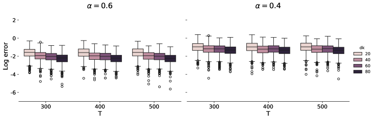
Figure 1: Boxplots of log estimation errors of $\widehat{f}_{T}$.

5.2 Factor Estimator Distribution

Next, we conduct simulations to assess the asymptotic normality of $\widehat{f}_{t}$, as stated in Theorem 3.1, and to evaluate the proposed covariance matrix estimator in Theorem 3.5. We vary $d_{k}$ in $\{40,60,80\}$ and let $T=800+\lceil d^{3/4}\rceil$.

Specifically, we use the SCAD thresholding function developed by Fan and Li, (2001), defined as

$${\cal T}(z)=\begin{cases}\operatorname{sgn}(z)(|z|-\lambda)_{+}&\text{if }|z|>a\lambda\\ \left[(a-1)z-\operatorname{sgn}(z)a\lambda\right]/(a-2)&\text{if }2\lambda<|z|\leq a\lambda\\ z&\text{if }|z|\leq 2\lambda,\end{cases}$$

where we set $a=3.7$ as suggested in Fan and Li, (2001). The threshold $\lambda$ is set to $\sqrt{\log(d)/T}+\sqrt{1/d}$.

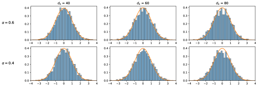
Figure 2: Sample distribution of $\widehat{\Sigma}_{Be}^{-1/2}(\widehat{\widetilde{f}}_{t}-\widetilde{f}_{t})$ over 2000 repetitions. The orange line is the pdf of standard normal.

Figures 2 shows the distribution of $\widehat{\Sigma}_{Be}^{-1/2}\widehat{S}(\widehat{f}_{T}-Hf_{T})$ over 2000 repetitions under two factor strengths. We note that the distribution of $\widehat{f}_{T}$ approximates the standard normal distribution, which validates Theorem 3.2. Furthermore, the result remains robust to cross-sectional dependence, supporting the effectiveness of the proposed thresholding covariance matrix estimation.

5.3 Prediction Interval

In this section, we examine the prediction intervals for $y_{T+1|T}$ constructed based on Theorem 3.4. The target variable $y_{t+1}$ is generated as

$$y_{t+1}=\beta_{0}+\beta_{1}^{\top}f_{t}+\epsilon_{t+1},$$

where $\beta_{0}=0.5$ and $\beta_{1}=\left(0.5,0.5,0.5\right)$. The idiocyncratic error $\epsilon_{t+1}$ is drawn independently from ${\cal N}(0,\nu_{t})$ with $\nu_{t}$ drawn independently from $U[0.5,1.5]$.

Set $d_{1}=d_{2}\in\{20,40,60,80,120,160\}$ and $T=800+\lceil d^{3/4}\rceil$, with a confidence level of 0.95. We assess the finite-sample performance of the prediction interval for $\widehat{y}_{T+1|T}$ proposed in Equation (16) and compare it with the vector PCA method of Bai and Ng, (2006). For this comparison, we apply the classical PCA method to the vectorized tensor $x_{t}:=\vec{(}{\cal X}_{t})\in\mathbb{R}^{d}$ and construct the confidence interval following Bai and Ng, (2006) and Bai and Ng, (2023):

$$\quad\left(\widehat{y}_{T+h|T}-q_{1-2/\alpha}\widehat{\sigma}_{y_{T+h|T},pca},\quad\widehat{y}_{T+h|T}+q_{1-2/\alpha}\widehat{\sigma}_{y_{T+h|T},pca}\right),$$ (23)

where $\widehat{\sigma}^{2}_{y_{T+h|T},pca}=\frac{1}{T}\widehat{z}_{T}^{(pca)\top}\ \widehat{\operatorname*{A\!var}}(\widehat{\beta}^{(pca)})\widehat{z}_{T}^{(pca)\top}+\frac{1}{d}\widehat{\beta}_{1}^{(pca)\top}\widehat{\operatorname*{A\!var}}(\widehat{f}_{T}^{(pca)})\widehat{\beta}_{1}^{(pca)\top}$. The variance estimator for $\widehat{f}_{T}^{(pca)}$ is given by

$$\widehat{\operatorname*{A\!var}}(\widehat{f}_{T}^{(pca)})=\tilde{V}^{-1}\widehat{\Gamma}_{t}\tilde{V}^{-1},$$

where $\tilde{V}$ is a diagonal matrix with diagonal elements equal to the top $r$ eigenvalues of $\frac{1}{dT}\sum_{t=1}^{T}x_{t}x_{t}^{\top}$, and $\widehat{z}_{T}^{(pca)}$, $\widehat{\beta}^{(pca)}$, and $\widehat{f}_{T}^{(pca)}$ are the corresponding PCA estimators. We consider two types of $\widehat{\Gamma}_{t}$. The first one is the $\widehat{A}^{(PCA)^{\top}}\widehat{\Sigma}^{({\cal T})}_{e,pca}\widehat{A}^{(PCA)}$ where $\widehat{A}^{(PCA)}$ are factor loadings estimated via PCA and $\widehat{\Sigma}_{e,pca}^{({\cal T})}$ is the proposed thresholding estimator of the covariance matrix of error terms for PCA. The second one is the HAC-type estimator proposed by Bai and Ng, (2006) and Bai and Ng, (2023):

$$\widehat{\Gamma}_{t}^{(HAC)}=\frac{1}{n}\sum_{j=1}^{n}\sum_{l=1}^{n}\widehat{A}_{j:}^{(\text{PCA})}\widehat{A}_{l:}^{\top(\text{PCA})}\frac{1}{T}\sum_{t=1}^{T}\widehat{e}_{jt}^{(\text{PCA})}\widehat{e}_{lt}^{(\text{PCA})},$$

where $\widehat{A}_{j:}^{(\text{PCA})}$ and $\widehat{e}_{jt}^{(\text{PCA})}$ are factor loadings and errors estimated via PCA, respectively. The tuning parameter is set as $n=\min\{\sqrt{d},\sqrt{T}\}$ as suggested by Bai and Ng, (2006). For both CP and PCA approach, $\operatorname*{A\!var}(\widehat{\beta})$ is estimated using Equation (14)

Table 1 shows the coverage rates of three estimated prediction intervals under two different values of $\alpha$, with a confidence level $95\%$. For $\alpha=0.6$, the coverage rates for the CP-based approach are close to the nominal level. For $\alpha=0.4$, the coverage rate is slightly lower when $d_{k}=20$ but converges to the nominal level as $d_{k}$ increases. In contrast, the PCA-based approach fails to produce reliable prediction intervals: its coverage rates deviate significantly from the nominal level and show no improvement with increasing $d_{k}$.

Table 1: Coverage rate of CP and PCA prediction intervals

	$\alpha=0.6$			$\alpha=0.4$
dk	CP	PCA(T)	PCA(H)	CP	PCA(T)	PCA(H)
20	0.925	0.783	0.731	0.880	0.456	0.426
40	0.923	0.602	0.654	0.896	0.361	0.393
60	0.935	0.716	0.723	0.921	0.420	0.421
80	0.939	0.696	0.722	0.924	0.367	0.381
120	0.939	0.727	0.739	0.932	0.391	0.396
160	0.960	0.774	0.789	0.954	0.398	0.406

Notes: (1) PCA(T) and PCA(H) refer to the prediction interval constructed using the PCA approach, where the covariance matrix of the factors is estimated via the proposed thresholding covariance estimator and the HAC-type estimator proposed by Bai and Ng, (2006) and Bai and Ng, (2023), respectively. (2) The nominal confidence level is $95\%$.

5.4 Multi-Source Factor-Augmented Sparse Regression

In this section, we evaluate the convergence rate of $\widehat{\beta}_{0}$ and $\widehat{y}_{T+1|T}$ in Theorem 4.1. Consider the following DGP for $y_{t+h}$ and $w_{t}\in\mathbb{R}^{p}$:

$$y_{t+1} =\beta_{0}^{\top}w_{t}+\beta_{1}^{\top}z_{t}+\epsilon_{t+1},$$

$$w_{t} =\Lambda z_{t}+V_{t},$$

where $z_{t}=\left(1,f_{t}^{\top}\right)\in\mathbb{R}^{r+1}$. We set the predictor dimension to $p=200$, with the first three elements of $\beta_{0}$ equal to $0.5$ and the remaining elements set to 0. Each entry of $\Lambda$ is drawn from the uniform distribution $U[-1,1]$, and the entries of $V_{t}$ are generated independently from $N(0,1)$. The idiosyncratic errors $\epsilon_{t+h}$ follow the same setting as in Section 5.3. We fix $d_{1}=d_{2}=40$ and vary $T$.

In this setting, the rate of $\|\widehat{\beta}_{0}-\beta_{0}\|_{1}$ is bounded above by $p_{0}\sqrt{\log(p)/T}$, while the forecast error $\left|\widehat{y}_{T+h|T}-y_{T+h|T}\right|$ is bounded above by $p_{0}\log(p)/\sqrt{T}$, given $\nu_{5}=2$ for Gaussian $V_{T}$. We choose $T$ such that $p_{0}\sqrt{\log(p)/T}$ takes values on a uniform grid in $[0.15,0.5]$, which implies that $p_{0}\log(p)/\sqrt{T}$ ranges in $(0.34,1.15)$. The tuning parameter for the LASSO regression is fixed at $\sqrt{\log(d)/T}+1/\widehat{s_{r}}$, where $\widehat{s_{r}}$ is the estimated weakest factor signal, $s_{r}$.

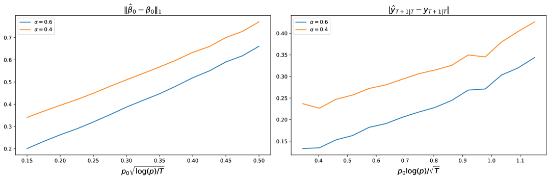
Figure 3: Estimation error of $\beta_{0}$ and prediction error of $y_{T+h|T}$ over 1000 repetitions under strong and weak factor setting.

Figure 3 reports the estimation and prediction errors. The results provide further support for the theoretical findings established in Section 4.

6 Empirical Application

Understanding trade flow patterns and forecasting their dynamics are essential for policymaking, firm optimization, and risk management. Trade data inherently form a dynamic sequence of tensor variates, which can capture network-like structures, underlie common dynamics, and reveal intricate interaction patterns. In this section, we consider a diffusion index forecast based on the CP tensor factor model for international trade data, providing a unified framework to estimate global trade factors and predict future variations in US trade.

6.1 Data and sample

We analyze monthly bilateral import and export volumes of commodity goods among 24 countries and regions from January 1999 to December 2018, using data from the International Monetary Fund Direction of Trade Statistics (IMF-DOTS). The countries and regions included in the dataset are: Australia (AU), Canada (CA), China Mainland (CN), Denmark (DK), Finland (FI), France (FR), Germany (DE), Hong Kong (HK), Indonesia (ID), Ireland (IE), Italy (IT), Japan (JP), Korea (KR), Malaysia (MY), Mexico (MX), Netherlands (NL), New Zealand (NZ), Singapore (SG), Spain (ES), Sweden (SE), Taiwan (TW), Thailand (TH), United Kingdom (GB), and the United States (US).

In our study, we employ the diffusion index forecast model with a CP low rank structure, as defined in (1) and (2). Specifically, we represent the trade data as a $24\times 24$ two-dimensional tensor, where each element $x_{i,j,t}$ denotes the monthly variation of exports from country $i$ to country $j$ at month $t$. For simplicity, self-exports are set to zero, i.e., $x_{i,i,t}=0$ for all $i$ and $t$. The target variables for our analysis are the monthly variation of US aggregate export and import to/from in-sample countries, denoted by $y_{t}^{ex}$ and $y_{t}^{im}$, respectively.

The number of common factors is determined using the eigen ratio-based method proposed by Ahn and Horenstein, (2013) and Chen et al., 2024a , which identifies four common factor explaining 51.1% of the total variance. Let $f_{t}$ denote the common factor extracted from the growth rate of bilateral trade. We then construct one-month-ahead forecasts for yearly growth of US aggregate exports and imports using the following regression:

$$\begin{split}y_{t+1}^{(ex)}&=\beta_{00}^{(ex)}+\beta_{01}^{(ex)}y_{t}^{(ex)}+\beta_{02}^{(ex)}y_{t}^{(im)}+\beta_{1}^{(ex)\top}f_{t}+\epsilon_{t+1}^{(ex)},\\ y_{t+1}^{(im)}&=\beta_{00}^{(im)}+\beta_{01}^{(im)}y_{t}^{(ex)}+\beta_{02}^{(im)}y_{t}^{(im)}+\beta_{1}^{(im)\top}f_{t}+\epsilon_{t+1}^{(im)}.\end{split}$$ (24)

6.2 In-sample analysis

Table 2: In-sample estimation results for monthly variations in US exports and imports

	Const	$y_{t}^{(ex)}$	$y_{t}^{(im)}$	$\widehat{f}_{1t}$	$\widehat{f}_{2t}$	$\widehat{f}_{3t}$	$\widehat{f}_{4t}$	$R^{2}$
$y_{t+1}^{(ex)}$
(a)	294.066	-0.325	-0.069					0.163
	(0.97)	(-3.48)	(-1.06)
(b)	384.766			0.726	-0.234	0.422	-0.125	0.289
	(1.363)			(6.73)	(-2.13)	(2.99)	(-0.74)
(c)	365.062	-0.989	0.337	1.118	0.347	0.6	1.179	0.402
	(1.4)	(-5.91)	(3.57)	(7.13)	(2.55)	(4.39)	(3.0)
$y_{t+1}^{(im)}$
(a)	586.208	-0.056	-0.307					0.114
	(1.31)	(-0.41)	(-3.21)
(b)	613.43			0.906	0.243	0.86	-0.457	0.211
	(1.45)			(5.61)	(1.47)	(4.07)	(-1.81)
(c)	597.329	-1.376	-0.069	0.759	0.941	1.21	2.4	0.301
	(1.49)	(-5.35)	(-0.47)	(3.15)	(4.5)	(5.76)	(3.97)

Note: The table reports results from the in-sample diffusion index model of monthly variation in US total export and import to countries in the dataset on lagged variables named in the first row. $\widehat{f}_{it}$ is the $i$-th common factor extracted from the bilateral trade flow tensor data. The t-values are reported in parentheses. Coefficients that are statistically significant at the 5% level are in bold.

Table 2 reports the in-sample forecast results based on Equation (24). As a benchmark, regression (a) predicts each target variable using only the first lag of changes in US exports and imports. In contrast, regression (b) demonstrates that incorporating common factors extracted from the tensor data significantly increases predictive power compared to using lagged values alone. Specifically, the common factors explain $29\%$ the variation in monthly export changes and 21% of the variation in import changes. Regression (c) integrates both the lagged target variables and the common factors, leading to a substantial improvement in explanatory power, with R-squared values increasing to 40% for US exports and 30% for imports. Moreover, all four common factors are statistically significant predictors for both trade flows. These findings highlight the crucial role of common factors derived from the tensor data in enhancing the accuracy of monthly US export and import forecasts.

Since the factors in the CP tensor model are identified only up to sign changes, it is meaningful to explore their economic interpretation. To characterize these factors, we examine their correlations with monthly variations in bilateral trade flows among the selected countries. These correlations are visualized in the heatmap shown in Figure 4, where stronger correlations between a factor and bilateral trade flows are indicated by deeper blue shades.

The heatmap reveals distinct regional patterns for each factor. Factor 1 is closely associated with exports from Asian countries to the rest of the dataset, with the highest correlation observed in exports from CN. Factor 2 is highly correlated with China’s imports from most countries in the dataset and also shows notable correlations with trade flows among key Asian economies, including CN, KR, JP, and SG. Factor 3 is mainly correlated with bilateral trade flows among European countries, while Factor 4 predominantly captures trade flows within North America, specifically among US, CA and MX. In summary, Factors 1 and 2 contain information on trade flows within Asia, particularly involving China. Factor 3 relates to trade dynamics within Europe, and Factor 4 captures variations in trade among North American countries. The in-sample analysis in Section 6.2 demonstrates that these factors are not only economically interpretable but also provide significant predictive power for monthly variations in US exports and imports.

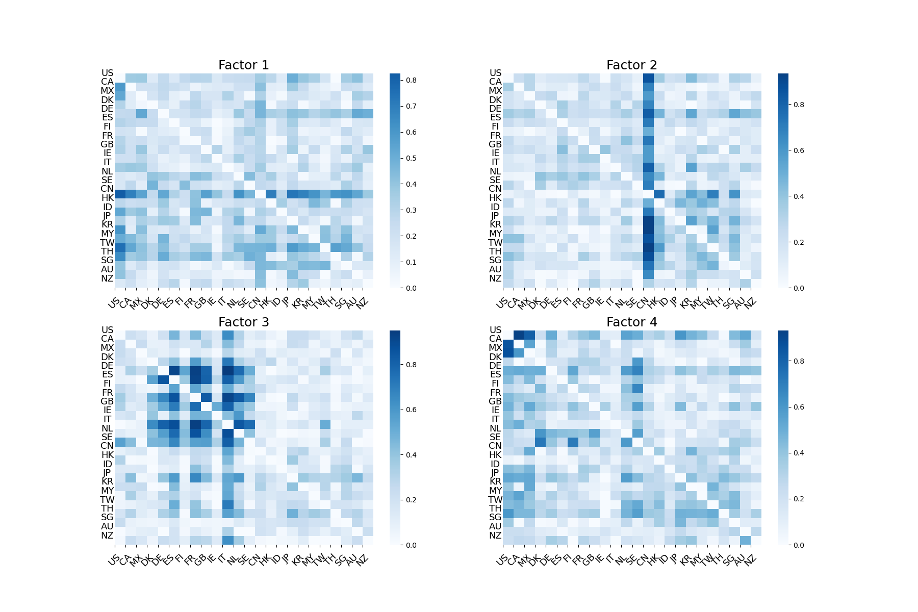
Figure 4: Heatmap of the absolute value of correlation between the common factors and the monthly variation in bilateral tradeflow among selected countries. The saturation represents the correlation strength, with high saturation indicating a stronger correlation.

6.3 Out-of-sample analysis

In the section, we evaluate the out-of-sample performance of the diffusion index model (24) based on the CP low rank structure and compare it with alternative methods, in particular the vector factor model studied by Bai and Ng, (2006). In addition to Model (24), we incorporate 126 macroeconomic variables from FRED-MD (McCracken and Ng,, 2016) and up to 12 lags of US aggregate exports and imports. This allows us to access the performance of MS-FASR, introduced in Section 4 and investigate whether including US macroeconomic variables and additional lags of the target variables improves the out-of-sample forecast of US aggregate exports and imports. The MS-FASR model is specified as follows:

$$\begin{split}y_{t+1}^{(ex)}&=\beta_{00}^{(ex)}+\beta_{01}^{(ex)}y_{t}^{(ex)}+\beta_{02}^{(ex)}y_{t}^{(im)}+\beta_{1}^{(ex)\top}f_{t}+\beta_{2}^{(ex)\top}w_{t}+\epsilon_{t+1}^{(ex)},\\ y_{t+1}^{(im)}&=\beta_{00}^{(im)}+\beta_{01}^{(im)}y_{t}^{(ex)}+\beta_{02}^{(im)}y_{t}^{(im)}+\beta_{1}^{(im)\top}f_{t}+\beta_{2}^{(im)\top}w_{t}+\epsilon_{t+1}^{(im)},\end{split}$$ (25)

where $w_{t}\in\mathbb{R}^{148}$ includes 126 macroeconomic variables and lagged US aggregate exports and imports from lag 2 to lag 12.

The out-of-sample analysis follows an expanding-window approach, where model parameters are re-estimated as new data become available. The process begins with an initial five-year sample from December 1999 to December 2004. Factors and parameters are estimated using data from December 1999 to November 2004, and the model is then used to forecast monthly variations in US aggregate exports and imports for December 2004. This procedure is repeated iteratively until the end of the sample, resulting in a total of 169 monthly forecasts from December 2004 to December 2018.

The tuning parameter $\lambda$ is selected via an expanding forecast validation scheme following Song and Bickel, (2011) and Han et al., (2015), which is appropriate for time-series settings. Specifically, we divide the sample into an initial training subsample $t=1,\ldots,\lceil\gamma T\rceil$ and a validation sample $t=\lceil\gamma T\rceil+1,\ldots,T$, with $\gamma=0.8$. For each candidate penalty $\lambda_{k}$, the model is recursively re-estimated and used to generate one-step-ahead forecasts over the validation period. The value of $\lambda_{k}$ that minimizes the mean squared prediction error is selected.

We compare the performance of Model (24) and Model (25) against various alternative methods:

• Benchmark: Predicts the target variable using only the first lag of US exports and imports along with a constant;

• DI(CP): Model (24) with factors estimated by CC-ISO;

• DI(PCA): Model (24) with factors estimated via PCA on $\vec{\left(}{\cal X}_{t}\right)$;

• MS-FASR(CP): Model (25) with factors estimated by CC-ISO;

• MS-FASR(PCA): Model (25) with factors estimated via PCA on $\vec{\left(}{\cal X}_{t}\right)$;

• DI(CP) + DI(w): $y_{t+1}^{(\cdot)}=\beta_{00}^{(\cdot)}+\beta_{01}^{(\cdot)}y_{t}^{(ex)}+\beta_{02}^{(\cdot)}y_{t}^{(im)}+\beta_{1}^{(\cdot)\top}f_{t}+\beta_{2}^{(\cdot)\top}f_{t}^{(w)}+\epsilon_{t+1}^{(\cdot)}$, where $f_{t}^{(w)}\in\mathbb{R}^{r_{w}}$ consists of factors extracted from $w_{t}$ via PCA and $f_{t}$ is estimated using CC-ISO;

• DI(PCA) + DI(w): Same as DI(CP) + DI(w) but with $f_{t}$ estimated via PCA on $\vec{\left(}{\cal X}_{t}\right)$;

• LASSO(w): $y_{t+1}^{(\cdot)}=\beta_{00}^{(\cdot)}+\beta_{01}^{(\cdot)}y_{t}^{(ex)}+\beta_{02}^{(\cdot)}y_{t}^{(im)}+\beta_{2}^{(\cdot)\top}w_{t}+\epsilon_{t+1}^{(ex)}$, where $\beta_{2}$ is estimated with an $\ell_{1}$-norm constraint.

Table 3 presents the Mean square error (MSE) ratios of the one-month-ahead out-of-sample forecast for each model relative to the benchmark. It also presents p-values from the forecast comparison tests of Diebold and Mariano, (1995) (DM). These tests are one-sided, with the following alternatives:

• DM(Benchmark): Competing methods outperform the benchmark model.

• DM(I): DI(CP) is more accurate than DI(PCA).

• DM(II): MS-FASR(CP) is more accurate than competing methods.

Our findings indicate that, for both exports and imports, MS-FASR(CP) achieves the lowest MSE among all the methods considered. First, MS-FASR(CP) significantly outperforms LASSO(w), reinforcing our in-sample results that common factors extracted from tensor data are valuable for predicting US export and import variations. Furthermore, MS-FASR(CP) outperforms both DI(CP) and DI(PCA) with DM test p-values smaller than any conventional significance level, suggesting that macroeconomic variables provide additional predictive power. Additionally, MS-FASR(CP) also outperforms DI(CP) + DI(w) and DI(PCA) + DI(w) models, which attempt to incorporate factors from multiple sources. This result provides strong empirical support for combining the CP tensor model with sparse regression. Notably, between CP and PCA, DI(CP) significantly outperforms DI(PCA); MS-FASR(CP) modestly improves upon MS-FASR(PCA), consistent with the theoretical argument in Remark 4.3.

The superior empirical performance of the MS-FASR method can be attributed to its ability to integrate multiple sources of information in a statistically coherent and efficient way. Specifically, the method jointly exploits (i) low-dimensional factors extracted from the tensor predictor, which capture common cross-country dynamics, and (ii) a high-dimensional set of macroeconomic predictors $w_{t}$, which provide complementary, country-specific signals. Unlike conventional diffusion-index regressions, MS-FASR selectively penalizes only the coefficients on $w_{t}$ while keeping factor components unpenalized. This structure preserves systematic global information from the tensor factors while preventing overfitting from noisy or redundant local predictors. Moreover, the residual-on-residual estimation step ensures that the penalized regression operates on information orthogonal to the factor space, mitigating multicollinearity and enhancing out-of-sample stability. Competing models either rely solely on factor information or treat all predictors symmetrically, which can reduce forecasting efficiency when predictive sources are heterogeneous. MS-FASR’s hybrid structure thus allows it to combine global coherence with local adaptability, yielding substantial gains in predictive accuracy.

To quantify the relative contributions of global and local information, we conduct a two-component Shapley attribution (Shapley,, 1953) that decomposes the total gain in forecast accuracy relative to the benchmark into contributions from local predictors ($w_{t}$) and global factors ($f_{t}$). The result shows that both local and global information contribute meaningfully to MS-FASR’s forecasting gains, with local predictors accounting for a slightly larger share. For exports, $54.5\%$ of the total MSE reduction is attributed to local information and $45.5\%$ to global factors; for imports, the shares are $61.3\%$ and $38.7\%$, respectively. This suggests that while local variation remains somewhat more influential, global factors also provide substantial complementary information, particularly for export forecasts.

Table 3: MSE ratios of out-of-sample forecasts

	DI(CP)	DI(PCA)	MS-FASR(CP)	MS_FASR(PCA)	DI(CP) + DI(w)	DI(PCA) + DI(w)	LASSO(w)
Export
MSE ratio	0.7733	0.8207	0.4354	0.449	0.8574	0.9205	0.6951
DM(Benchmark)	0.0108	0.0371	<0.0001	<0.0001	0.1182	0.2574	0.0034
DM(I)	-	0.0599	-	-	-	-	-
DM(II)	<0.0001	<0.0001	-	0.2356	<0.0001	<0.0001	0.0001
Import
MSE ratio	0.8159	0.8965	0.5156	0.5116	1.0079	1.0526	0.6441
DM(Benchmark)	0.0012	0.028	<0.0001	<0.0001	0.4751	0.286	0.0001
DM(I)	-	0.0015	-	-	-	-	-
DM(II)	<0.0001	<0.0001	-	0.4407	<0.0001	<0.0001	0.0083

Notes: (1) The table reports the out-of-sample MSE ratios relative to the benchmark model, which only includes $y_{t}=(y_{t}^{(ex)},y_{t}^{(im)})^{\top}$ and a constant. (2) The MSE Ratio row shows the ratio of each method’s MSE to that of the benchmark model; DM(Benchmark) reports DM test p-values with the alternative being that the competing method is more accurate than the benchmark model; DM(I) reports DM test p-values with the alternative being that DI(CP) outperforms DI(PCA); DM(II) reports DM test p-values with the alternative being that MS-FASR(CP) outperforms the competing method. (3) The number of factors is selected by the unfolded eigenvalue ratio method by Chen et al., 2024a . (4) The tuning parameter $\lambda$ for LASSO and MS-FASR is selected by the EV scheme.

7 Conclusion

Factor models are powerful tools for extracting meaningful information from high-dimensional data, which can then be used for prediction. This paper studies the case where the data naturally take the form of a tensor and can be represented by CP decomposition. We develop inferential theories for factor estimation and predictive intervals in the diffusion index forecasting model. We establish that the least squares estimates from predictive regressions are $\sqrt{T}$-consistent and asymptotically normal, even in the presence of weaker factors. Furthermore, we show that the conditional mean remains consistent and asymptotically normal, with its convergence rate determined by $T$ and the strength of the weakest factor. For predictive inference, we propose a consistent estimator for the high-dimensional covariance matrix of cross-sectionally correlated and heteroskedastic errors.

Additionally, we consider settings where multiple data sources with different structures are available and introduce the MS-FASR model, which effectively integrates information across datasets. Simulation studies confirm our theoretical results, and an empirical application demonstrates that leveraging the tensor structure enhances predictive performance. Our findings suggest that incorporating tensor-based factor extraction can lead to substantial improvements over existing forecasting methods.

Supplementary Material of
“Diffusion Index Forecast with Tensor Data”

Appendix A Proofs of Theorems

Proof of Theorem 3.1.

Let $\widehat{\widetilde{f}}_{it}=\widehat{s}_{i}\widehat{f}_{it}$ and $\widetilde{f}_{t}=s_{i}f_{it}$. For $(iii)$, since

$$\|\widehat{\widetilde{f}}_{t}-\widetilde{f}_{t}\|_{2}=\left\|\sum_{i=1}^{r}\widehat{\widetilde{f}}_{it}-\widetilde{f}_{it}\right\|_{2}\leq\sum_{i=1}^{r}\|\widehat{\widetilde{f}}_{it}-\widetilde{f}_{it}\|_{2},$$

it suffices to show that $|\widehat{\widetilde{f}}_{it}-\widetilde{f}_{it}|=O_{p}(s_{i}\psi)$. The same logic can be applied to $(iv)$ and $(v)$.

$$\widehat{\widetilde{f}}_{it}-\widetilde{f}_{it} ={\cal X}_{t}\times_{k=1}^{K}\widehat{b}_{ik}^{\top}-\widetilde{f}_{it}$$

$$=\widetilde{f}_{it}(\prod_{k=1}^{K}a_{ik}^{\top}\widehat{b}_{ik}-1)+\sum_{j\neq i}^{r}\widetilde{f}_{jt}(\prod_{k=1}^{K}a_{jk}^{\top}\widehat{b}_{ik})+{\cal E}_{t}\times_{k=1}^{K}\widehat{b}_{ik}^{\top}$$

$$:=\Pi_{1}+\Pi_{2}+\Pi_{3}.$$

For $\Pi_{1}$, by construction of $\widehat{b}_{ik}$, $\widehat{a}_{ik}^{\top}\widehat{b}_{ik}=1$.

$$a_{ik}^{\top}\widehat{b}_{ik}=a_{ik}^{\top}\widehat{b}_{ik}-1+1=(\widehat{a}_{ik}-a_{ik})^{\top}\widehat{b}_{ik}+1\leq\|\widehat{a}_{ik}-a_{ik}\|_{2}\|\widehat{b}_{ik}\|_{2}+1.$$ (26)

To bound $\|\widehat{a}_{ik}-a_{ik}\|_{2}$,

$$\|\widehat{a}_{ik}-a_{ik}\|_{2}^{2} =(\widehat{a}_{ik}-a_{ik})^{\top}(\widehat{a}_{ik}-a_{ik})$$

$$=2(1-a_{ik}^{\top}\widehat{a}_{ik})$$

$$\leq 2\left(1-(a_{ik}^{\top}\widehat{a}_{ik})^{2}\right)$$

$$=2\|\widehat{a}_{ik}\widehat{a}_{ik}^{\top}-a_{ik}a_{ik}^{\top}\|_{2}^{2},$$

which yields

$$\|\widehat{a}_{ik}-a_{ik}\|_{2}\leq\sqrt{2}\psi.$$ (27)

To bound $\|\widehat{b}_{ik}\|_{2}$, denote $A_{k}^{\top}A_{k}=\Sigma_{k}$ and $\widehat{A}_{k}^{\top}\widehat{A}_{k}=\widehat{\Sigma}_{k}$. Observe that

$$\|\widehat{b}_{ik}\|_{2} =\|\widehat{A}_{k}(\widehat{A}_{k}^{\top}\widehat{A}_{k})^{-1}e_{1}\|_{2}$$

$$=e_{1}^{\top}(\widehat{A}_{k}^{\top}\widehat{A}_{k})^{-1}\widehat{A}_{k}^{\top}\widehat{A}_{k}(\widehat{A}_{k}^{\top}\widehat{A}_{k})^{-1}e_{1}$$

$$=e_{1}^{\top}(\widehat{A}_{k}^{\top}\widehat{A}_{k})^{-1}e_{1}$$

$$\leq\|\widehat{\Sigma}_{k}^{-1}\|_{2}$$

$$=\left\|\left(\Sigma_{k}-(\Sigma_{k}-\widehat{\Sigma}_{k})\right)^{-1}\right\|_{2}$$

$$\leq\frac{1}{\lambda_{min}\left(\Sigma_{k}-(\Sigma_{k}-\widehat{\Sigma}_{k})\right)}$$

$$\leq\frac{1}{\lambda_{min}(\Sigma_{k})-\lambda_{max}(\Sigma_{k}-\widehat{\Sigma}_{k})}$$

$$\leq\frac{1}{\lambda_{min}(\Sigma_{k})-\|\widehat{\Sigma}_{k}-\Sigma_{k}\|_{2}},$$ (28)

where the second last inequality is by Weyl’s inequality. For $\Sigma_{k}$, for all $1\leq i\leq r$,

$$\left|\lambda_{i}(\Sigma_{k})-1\right|\leq\delta,$$

which implies $\lambda_{min}(\Sigma_{k})\geq 1-\delta$ and $\lambda_{max}(\Sigma_{k})\leq 1+\delta_{k}$. From the bound of $\lambda_{max}(\Sigma_{k})$, we have $\|A_{k}\|_{2}=\sqrt{\|A_{k}^{\top}A_{k}\|_{2}}\leq\sqrt{1+\delta_{k}}$. For $\|\widehat{\Sigma}_{k}-\Sigma_{k}\|_{2}$,

$$\|\widehat{\Sigma}_{k}-\Sigma_{k}\|_{2} =\|\widehat{A}_{k}^{\top}\widehat{A}_{k}-A_{k}^{\top}A_{k}\|_{2}$$

$$=\|(\widehat{A}_{k}-A_{k})^{\top}(\widehat{A}_{k}^{\top}-A_{k})+\widehat{A}_{k}^{\top}A_{k}+A_{k}^{\top}\widehat{A}_{k}-2A_{k}^{\top}A_{k}\|_{2}$$

$$\leq\|\widehat{A}_{k}-A_{k}\|_{2}^{2}+2\|(\widehat{A}_{k}-A_{k})^{\top}A_{k}\|_{2}$$

$$\leq\|\widehat{A}_{k}-A_{k}\|_{2}^{2}+2\|\widehat{A}_{k}-A_{k}\|_{2}\|A_{k}\|_{2}.$$ (29)

Note

$$\|\widehat{A}_{k}-A_{k}\|_{2} =\max_{\|x\|=1}\|(\widehat{A}_{k}-A_{k})x\|_{2}$$

$$=\max_{\|x\|=1}\|\sum_{i=1}^{r}(\widehat{a}_{ik}-a_{ik})x_{i}\|_{2}$$

$$\leq\max_{\|x\|=1}\left(\sum_{i=1}^{r}\|\widehat{a}_{ik}-a_{ik}\|_{2}^{2}\right)^{\frac{1}{2}}\left(\sum_{i=1}^{r}x_{i}\right)^{\frac{1}{2}}$$

$$=\left(\sum_{i=1}^{r}\|\widehat{a}_{ik}-a_{ik}\|_{2}^{2}\right)^{\frac{1}{2}}$$

$$\leq\sqrt{2r}\psi.$$

Plug it to (A), we have

$$\|\widehat{\Sigma}_{k}-\Sigma_{k}\|_{2}\leq 2r\psi^{2}+2\sqrt{2r}\psi\sqrt{1+\delta_{k}}.$$

Plug it to (A), we have

$$\|\widehat{b}_{ik}\|_{2}\leq\frac{1}{1-\delta_{k}-2r\psi^{2}-2\sqrt{2r}\psi\sqrt{1+\delta_{k}}}.$$

As $r$ is fixed, we have

$$\|\widehat{b}_{ik}\|_{2}=O_{p}(1).$$ (30)

By (26) and (27), we have

$$a_{ik}^{\top}\widehat{b}_{ik}\leq\sqrt{2}\psi+1.$$ (31)

Therefore,

$$\Pi_{1}=\widetilde{f}_{it}\left(\prod_{k=1}^{K}a_{ik}^{\top}\widehat{b}_{ik}-1\right)\leq\widetilde{f}_{it}\left(\prod_{k=1}^{K}(\sqrt{2}\psi+1)-1\right)=O_{p}(s_{i}\psi).$$ (32)

For $\Pi_{2}$, similarly to $\Pi_{1}$, for $i\neq j$,

$$\widehat{a}_{jk}^{\top}\widehat{b}_{ik}=0.$$

So

$$a_{jk}^{\top}\widehat{b}_{ik}=(a_{jk}-\widehat{a}_{jk})^{\top}\widehat{b}_{ik}\leq\|\widehat{a}_{jk}-a_{jk}\|_{2}\|\widehat{b}_{ik}\|_{2}\lesssim\psi.$$

Therefore,

$$\sum_{j\neq i}f_{jt}(\prod_{k=1}^{K}a_{jk}^{\top}\widehat{b}_{ik})=O_{p}(s_{1}\psi^{K}).$$ (33)

For $\Pi_{3}$, denote $\widehat{g}_{ik}=\frac{\widehat{b}_{ik}}{\|\widehat{b}_{ik}\|_{2}}$ and $g_{ik}=\frac{b_{ik}}{\|b_{ik}\|_{2}}$.

$${\cal E}_{t}\times_{k=1}^{K}\widehat{b}_{ik} =\prod_{k=1}^{K}\|\widehat{b}_{ik}\|_{2}\cdot{\cal E}_{t}\times\widehat{g}_{ik}^{\top}$$

$$\leq\prod_{k=1}^{K}\|\widehat{b}_{ik}\|_{2}\cdot\max_{\|u_{k}\|_{2}=1}{\cal E}_{t}\times_{k=1}^{K}u_{k}^{\top}$$

$$\leq\prod_{k=1}^{K}\|\widehat{b}_{ik}\|_{2}\cdot\max_{\|u\|_{2}}u^{\top}\mbox{vec}({\cal E}_{t})$$

$$=\prod_{k=1}^{K}\|\widehat{b}_{ik}\|_{2}\cdot\max_{\|u\|_{2}}u^{\top}e_{t}.$$ (34)

By Assumption 3.1,

$$P\left(u^{\top}e_{t}>x\right) <\frac{u^{\top}{\mathbb{E}}\left[e_{t}e_{t}^{\top}\right]u}{x}$$

$$\leq\frac{\lambda_{1}(\Sigma_{e})}{x}\leq\frac{C_{0}}{x}.$$ (35)

Therefore,

$$\max_{\|u\|_{2}=1}u^{\top}e_{t}=O_{p}(1).$$

By (30) and (A), we have

$$\Pi_{3}=O_{p}(1).$$

Therefore, putting them all together:

$$\widehat{\widetilde{f}}_{it}-\widetilde{f}_{it}=O_{p}(s_{i}\psi+s_{1}\psi^{K}+1).$$

Since $r$ is fixed, by Assumption 3.2,

$$\|\widehat{\widetilde{f}}_{t}-\widetilde{f}_{t}\|_{2}=O_{p}(s_{1}\psi+1)=O_{p}(d^{1/2-\alpha_{r}}\sqrt{\frac{d_{max}}{T}}+\sqrt{\frac{d^{1-\alpha_{r}}}{T}}+d^{1/2-\alpha_{r}}+1),$$

Notice that

$$\widehat{f}_{it}-f_{it} =\widehat{s}_{i}^{-1}\widehat{\widetilde{f}}_{it}-f_{it}$$

$$=\widehat{s}_{i}^{-1}\left(\widehat{\widetilde{f}}_{it}-s_{i}f_{it}\right)+\left(\widehat{s}_{i}^{-1}-s_{i}^{-1}\right)s_{i}f_{it}$$

$$=\left(\widehat{f}_{it}-h_{i}f_{it}\right)+\left(\widehat{s}_{i}^{-1}-s_{i}^{-1}\right)\widetilde{f}_{it}.$$ (36)

So $\widehat{f}_{it}-f_{it}$ has one additional term involving $\widehat{s}_{i}$, compared with $\widehat{f}_{it}-h_{i}f_{it}$. For $\widehat{f}_{it}-h_{i}f_{it}$,

$$\widehat{f}_{it}-h_{i}f_{it} =(\widehat{s}_{i}^{-1}-s_{i}^{-1})(\widehat{\widetilde{f}}_{it}-\widetilde{f}_{it})+s_{i}^{-1}(\widehat{\widetilde{f}}_{it}-\widetilde{f}_{it})$$

$$=(\widehat{s}_{i}^{-1}-s_{i}^{-1})(\widehat{\widetilde{f}}_{it}-\widetilde{f}_{it})+O_{p}(\psi+\frac{1}{s_{i}}).$$ (37)

By Taylor expansion,

$$\widehat{s}_{i}^{-1}-s_{i}^{-1}=-\frac{1}{2}s_{i}^{-3}(\widehat{s}_{i}^{2}-s_{i}^{2})+\frac{3}{8}s_{i}^{-5}(\widehat{s}_{i}^{2}-s_{i}^{2})^{2}+O(s_{i}^{-7}(\widehat{s}_{i}^{2}-s_{i}^{2})^{3}).$$ (38)

To bound $\widehat{s}_{i}^{2}-s_{i}^{2}$, observe that

$$\widehat{s}_{i}^{2}-s_{i}^{2} =\frac{1}{T}\sum_{t=1}^{T}\widehat{\widetilde{f}}_{it}^{2}-{\mathbb{E}}\left[\widetilde{f}_{it}^{2}\right]$$

$$=\frac{1}{T}\sum_{t=1}^{T}(\widehat{\widetilde{f}}_{it}^{2}-\widetilde{f}_{it}^{2})+\frac{1}{T}\sum_{t=1}^{T}\left(\widetilde{f}_{it}^{2}-{\mathbb{E}}\left[\widetilde{f}_{it}^{2}\right]\right)$$

$$:=\Gamma_{2}+\Gamma_{1}.$$

For $\Gamma_{1}$, by Bernstein inequality for $\alpha$-mixing processes by Merlevède et al., (2011) and by assumption 3.1, for $\frac{1}{\gamma}=\frac{2}{\gamma_{1}}+\frac{1}{\gamma_{2}}$,

$$\begin{split}P\left[Ts_{i}^{-2}\left(\frac{1}{T}\sum_{t=1}^{T}(\widetilde{f}_{it}^{2}-s_{i}^{2})\geq x\right)\right]\leq T\exp\left(-\frac{x^{\gamma}}{c_{1}}\right)+&\exp\left(-\frac{x^{2}}{c_{2}T}\right)\\ &+\exp\left(-\frac{x^{2}}{c_{3}T}\exp\left(\frac{x^{\gamma(1-\gamma)}}{c_{4}(\log(x))^{\gamma}}\right)\right).\end{split}$$

Let $x\asymp\sqrt{T\log(T)}+(\log(T))^{1/\gamma}$. Then with probability at $\frac{1}{2}T^{-c_{2}}$,

$$s_{i}^{-2}\frac{1}{T}\sum_{t=1}^{T}(\widetilde{f}_{it}^{2}-s_{i}^{2})\geq\sqrt{\frac{\log(T)}{T}}+\frac{1}{T}\left(\log(T)^{1/\gamma}\right),$$

which implies

$$\Gamma_{1}=\frac{1}{T}\sum_{t=1}^{T}(\widetilde{f}_{it}^{2}-s_{i}^{2})=s_{i}^{2}O_{p}(\sqrt{\frac{1}{T}}).$$ (39)

For $\Gamma_{2}$, we consider the following general form:

$$\frac{1}{T}\sum_{t=1}^{T}\left(\widehat{\widetilde{f}}_{it}\widehat{\widetilde{f}}_{jt}-\widetilde{f}_{it}\widetilde{f}_{jt}\right).$$

Expanding it, we have

$$\frac{1}{T}\sum_{t=1}^{T}\left(\widehat{\widetilde{f}}_{it}\widehat{\widetilde{f}}_{jt}-\widetilde{f}_{it}\widetilde{f}_{jt}\right)$$

$$=\frac{1}{T}\sum_{t=1}^{T}\left({\cal X}_{t}\otimes{\cal X}_{t}\right)\times_{k=1}^{K}\widehat{b}_{ik}^{\top}\times_{k=K+1}^{2K}\widehat{b}_{jk}^{\top}-\widetilde{f}_{it}\widetilde{f}_{jt}$$

$$\begin{split}&=\frac{1}{T}\sum_{t=1}^{T}\left({\cal E}_{t}\otimes{\cal E}_{t}\right)\times_{k=1}^{K}\widehat{b}_{ik}^{\top}\times_{K+1}^{2K}\widehat{b}_{jk}^{\top}\\ &\quad+\frac{1}{T}\sum_{t=1}^{T}\widetilde{f}_{it}\widetilde{f}_{jt}\left(\prod_{k=1}^{K}a_{ik}^{\top}\widehat{b}_{ik}\prod_{k=1}^{K}a_{jk}^{\top}\widehat{b}_{jk}-1\right)\\ &\quad+\frac{1}{T}\sum_{t=1}^{T}\sum_{l_{1}\neq i}\sum_{l_{2}\neq j}\widetilde{f}_{l_{1}t}\widetilde{f}_{l_{2}t}\prod_{k=1}^{K}a_{l_{1}k}^{\top}\widehat{b}_{ik}\prod_{k=1}^{K}a_{l_{2}k}^{\top}\widehat{b}_{jk}\\ &\quad+\frac{1}{T}\sum_{t=1}^{T}\sum_{l\neq i}\widetilde{f}_{lt}\widetilde{f}_{jt}\prod_{k=1}^{K}a_{lk}^{\top}\widehat{b}_{ik}\prod_{k=1}^{K}a_{jk}^{\top}\widehat{b}_{jk}+\frac{1}{T}\sum_{t=1}^{T}\sum_{l\neq j}\widetilde{f}_{it}\widetilde{f}_{lt}\prod_{k=1}^{K}a_{ik}^{\top}\widehat{b}_{ik}\prod_{k=1}^{K}a_{lk}^{\top}\widehat{b}_{jk}\\ &\quad+\frac{1}{T}\sum_{t=1}^{T}\widetilde{f}_{it}\left(\prod_{k=1}^{K}a_{ik}^{\top}\widehat{b}_{ik}\right)\left({\cal E}_{t}\times_{k=1}^{K}\widehat{b}_{jk}^{\top}\right)+\frac{1}{T}\sum_{t=1}^{T}\widetilde{f}_{jt}\left(\prod_{k=1}^{K}a_{jk}^{\top}\widehat{b}_{jk}\right)\left({\cal E}_{t}\times_{k=1}^{K}\widehat{b}_{ik}^{\top}\right)\\ &\quad+\frac{1}{T}\sum_{t=1}^{T}\sum_{l\neq i}\widetilde{f}_{lt}\left(\prod_{k=1}^{K}a_{lk}^{\top}\widehat{b}_{ik}\right)\left({\cal E}_{t}\times_{k=1}^{K}\widehat{b}_{jk}^{\top}\right)+\frac{1}{T}\sum_{t=1}^{T}\sum_{l\neq j}\widetilde{f}_{lt}\left(\prod_{k=1}^{K}a_{lk}^{\top}\widehat{b}_{jk}\right)\left({\cal E}_{t}\times_{k=1}^{K}\widehat{b}_{ik}^{\top}\right)\\ \end{split}$$

$$=\sum_{i=1}^{9}\Delta_{i}.$$

For $\Delta_{1}$,

$$\Delta_{1} =\frac{1}{T}\sum_{t=1}^{T}{\cal E}_{t}\otimes{\cal E}_{t}\times_{k=1}^{K}\widehat{b}_{ik}^{\top}\times_{K+1}^{2K}\widehat{b}_{jk}^{\top}$$

$$=\left(\prod_{k=1}^{K}\|\widehat{b}_{ik}\|_{2}\prod_{k=1}^{K}\|\widehat{b}_{jk}\|_{2}\right)\frac{1}{T}\sum_{t=1}^{T}{\cal E}_{t}\otimes{\cal E}_{t}\times_{k=1}^{K}\widehat{g}_{ik}^{\top}\times_{k=K+1}^{2K}\widehat{g}_{jk}^{\top}.$$

By (30),

$$\prod_{k=1}^{K}\|\widehat{b}_{ik}\|_{2}\prod_{k=1}^{K}\|\widehat{b}_{jk}\|_{2}=O_{p}(1).$$

Expand the outer product, we have

$$\frac{1}{T}\sum_{t=1}^{T}{\cal E}_{t}\otimes{\cal E}_{t}\times_{k=1}^{K}\widehat{g}_{ik}^{\top}\times_{k=K+1}^{2K}\widehat{g}_{jk}^{\top}$$

$$=\frac{1}{T}\sum_{t=1}^{T}{\cal E}_{t}\otimes{\cal E}_{t}\times_{1}g_{i1}\times_{k=2}^{K}\widehat{g}_{ik}^{\top}\times_{k=K+1}^{2K}\widehat{g}_{jk}^{\top}+\frac{1}{T}\sum_{t=1}^{T}{\cal E}_{t}\otimes{\cal E}_{t}\times_{1}(\widehat{g}_{i1}-g_{i1})\times_{k=1}^{K}\widehat{g}_{ik}^{\top}\times_{k=K+1}^{2K}\widehat{g}_{jk}^{\top}$$

$$\begin{split}&\leq\frac{1}{T}\sum_{t=1}^{T}{\cal E}_{t}\otimes{\cal E}_{t}\times_{1}g_{i1}\times_{k=2}^{K}\widehat{g}_{ik}^{\top}\times_{k=K+1}^{2K}\widehat{g}_{jk}^{\top}\\ &\quad+\|\widehat{g}_{i1}-g_{i1}\|_{2}\max_{\|u_{ik}\|=\|u_{jk}\|_{2}=1}\frac{1}{T}\sum_{t=1}^{T}{\cal E}_{t}\otimes{\cal E}_{t}\times_{1}u_{i1}\times_{k=1}^{K}u_{ik}^{\top}\times_{k=K+1}^{2K}u_{jk}^{\top}\end{split}$$

$$\leq\cdots$$

$$\begin{split}&\leq\frac{1}{T}\sum_{t=1}^{T}{\cal E}_{t}\otimes{\cal E}_{t}\times_{k=1}^{K}g_{ik}^{\top}\times_{k=K+1}^{2K}g_{jk}^{\top}\\ &\quad+(\sum_{k=1}^{K}\|\widehat{g}_{ik}-g_{ik}\|_{2}+\sum_{k=1}^{K}\|\widehat{g}_{jk}-g_{jk}\|_{2})\max_{\|u_{ik}\|=\|u_{jk}\|_{2}=1}\frac{1}{T}\sum_{t=1}^{T}{\cal E}_{t}\otimes{\cal E}_{t}\times_{1}u_{i1}\times_{k=1}^{K}u_{ik}^{\top}\times_{k=K+1}^{2K}u_{jk}^{\top}.\end{split}$$

By Assumption 3.1,

$$\frac{1}{T}\sum_{t=1}^{T}{\cal E}_{t}\otimes{\cal E}_{t}\times_{k=1}^{K}g_{ik}^{\top}\times_{k=K+1}^{2K}g_{jk}^{\top}=g_{i}^{\top}\left(\frac{1}{T}\sum_{t=1}^{T}e_{t}e_{t}^{\top}\right)g_{j}=O_{p}(1).$$

By Chen et al., 2024a , $\|\widehat{g}_{ik}-g_{ik}\|_{2}\lesssim\psi$ if $r$ is fixed. Therefore, since $r$ and $K$ are fixed,

$$\sum_{k=1}^{K}\|\widehat{g}_{ik}-g_{ik}\|_{2}+\sum_{k=1}^{K}\|\widehat{g}_{jk}-g_{jk}\|_{2}\lesssim\psi.$$

Denote $\epsilon$-net for $S^{d_{k}-1}$ with ${\cal N}_{k}(\epsilon)$ for $1\leq k\leq K$. Then the cartesian product of $\epsilon$-net for $S^{d_{k}-1}$, $1\leq k\leq 2K$ form a $\sqrt{2K}\epsilon$-net for $S^{d_{1}-1}\times\cdots S^{d_{K}-1}\times S^{d_{1}-1}\times\cdots S^{d_{K}-1}$. Denote it with ${\cal N}(\sqrt{2K}\epsilon)$ and denote $u_{i}=\odot_{k=1}^{K}u_{ik}$ and $u_{j}=\odot_{k=1}^{K}u_{jk}$. By Corollary 4.2.13 and Lemma 4.4.1 in Vershynin, (2024), take $\epsilon=\frac{1}{3}$, we have $|{\cal N}(\sqrt{2K}\epsilon)|=49^{d_{1}+\cdots+d_{K}}\lesssim 7^{d_{max}}$ and

$$\max_{\|u_{ik}\|=\|u_{jk}\|_{2}=1}\frac{1}{T}\sum_{t=1}^{T}{\cal E}_{t}\otimes{\cal E}_{t}\times_{1}u_{i1}\times_{k=1}^{K}u_{ik}^{\top}\times_{k=K+1}^{2K}u_{jk}^{\top}\lesssim\max_{u_{ik},u_{jk}\in{\cal N}_{k}(\frac{1}{3\sqrt{2K}})}u_{i}^{\top}\left(\frac{1}{T}\sum_{t=1}^{T}e_{t}e_{t}^{\top}\right)u_{j}.$$

By Assumption 3.1 and Lemma B.12, for any conformable unit-norm vector $u_{i}$ and $u_{j}$, $u_{i}^{\top}e_{t}e_{t}^{\top}u_{j}$ is a general sub-exponential random variable with parameter $2/\nu_{1}$. By Theorem 1 in Merlevède et al., (2011) , for $\frac{1}{\eta_{1}}=\frac{2}{\nu_{1}}+\frac{1}{\gamma}$,

$$\mathbb{P}\left(u_{i}\left(\sum_{t=1}^{T}(e_{t}e_{t}^{\top}-{\mathbb{E}}\left[e_{t}e_{t}^{\top}\right])\right)u_{j}>x\right)\leq T\exp\left(-\frac{x^{\eta_{1}}}{c_{1}}\right)+\exp\left(-\frac{x^{2}}{c_{2}T}\right)+\exp\left(-\frac{x^{2}}{c_{3}T}\exp\left(\frac{x^{{\eta_{1}}(1-{\eta_{1}})}}{c_{4}(\log x)^{\eta_{1}}}\right)\right).$$

Let $x\asymp\sqrt{T(d_{max}+\log T)}+(d_{max}+\log T)^{1/{\eta_{1}}}$, by union bound and condition of Theorem 3.1, we have, with probability at least $1-\frac{1}{2}T^{-c_{2}}$,

$$\max_{\|u_{ik}\|=\|u_{jk}\|_{2}=1}\frac{1}{T}\sum_{t=1}^{T}{\cal E}_{t}\otimes{\cal E}_{t}\times_{1}u_{i1}\times_{k=1}^{K}u_{ik}^{\top}\times_{k=K+1}^{2K}u_{jk}^{\top}\lesssim\sqrt{\frac{d_{max}+\log(T)}{T}}+\frac{(d_{max}+\log T)^{1/{\eta_{1}}}}{T}+1,$$

which implies that

$$\max_{\|u_{ik}\|=\|u_{jk}\|_{2}=1}\frac{1}{T}\sum_{t=1}^{T}{\cal E}_{t}\otimes{\cal E}_{t}\times_{1}u_{i1}\times_{k=1}^{K}u_{ik}^{\top}\times_{k=K+1}^{2K}u_{jk}^{\top}=O_{p}\left(\sqrt{\frac{d_{max}}{T}}+\frac{d_{max}^{1/{\eta_{1}}}}{T}+1\right).$$

Therefore, we have

$$\Delta_{1}=O_{p}\left(1+\psi+\psi\left(\sqrt{\frac{d_{max}}{T}}+\frac{d_{max}^{1/{\eta_{1}}}}{T}\right)\right).$$ (40)

For $\Delta_{2}$, by (31),

$$\prod_{k=1}^{K}a_{ik}^{\top}\widehat{b}_{ik}\prod_{k=1}^{K}a_{jk}^{\top}\widehat{b}_{jk}=\left(1+O_{p}(\psi)\right)^{2K}=1+O_{p}(\psi).$$

Therefore

$$\Delta_{2} =\frac{1}{T}\sum_{t=1}^{T}\widetilde{f}_{it}\widetilde{f}_{jt}O_{p}(\psi)$$

$$\leq\left(\frac{1}{T}\sum_{t=1}^{T}\widetilde{f}_{it}^{2}\right)^{1/2}\left(\frac{1}{T}\sum_{t=1}^{T}\widetilde{f}_{jt}^{2}\right)^{1/2}O_{p}(\psi)$$

$$=\left(\frac{1}{T}\sum_{t=1}^{T}(\widetilde{f}_{it}^{2}-s_{i}^{2})+s_{i}^{2}\right)^{1/2}\left(\frac{1}{T}\sum_{t=1}^{T}(\widetilde{f}_{jt}^{2}-s_{j}^{2})+s_{j}^{2}\right)^{1/2}O_{p}(\psi)$$

$$=O_{p}(s_{i}s_{j}\psi).$$ (41)

The last step is based on (39).

For $\Delta_{3}$,

$$\Delta_{3} =\frac{1}{T}\sum_{t=1}^{T}\sum_{l_{1}\neq i}\sum_{l_{2}\neq j}\widetilde{f}_{l_{1}t}\widetilde{f}_{l_{2}t}\prod_{k=1}^{K}a_{l_{1}k}^{\top}\widehat{b}_{ik}\prod_{k=1}^{K}a_{l_{2}k}^{\top}\widehat{b}_{jk}$$

$$=\frac{1}{T}\sum_{t=1}^{T}\left(\sum_{l_{1}\neq i}f_{l_{1}t}\prod_{k=1}^{K}a_{l_{1}k}^{\top}\widehat{b}_{ik}\right)\left(\sum_{l_{2}\neq j}f_{l_{2}t}\prod_{k=1}^{K}a_{l_{2}k}^{\top}\widehat{b}_{jk}\right)$$

$$\leq\left(\frac{1}{T}\sum_{t=1}^{T}\left(\sum_{l_{1}\neq i}f_{l_{1}t}\prod_{k=1}^{K}a_{l_{1}k}^{\top}\widehat{b}_{ik}\right)^{2}\right)^{1/2}\left(\frac{1}{T}\sum_{t=1}^{T}\left(\sum_{l_{2}\neq j}f_{l_{2}t}\prod_{k=1}^{K}a_{l_{2}k}^{\top}\widehat{b}_{jk}\right)^{2}\right)^{1/2}$$

$$\leq\left(\sum_{l_{1}\neq i}\sum_{l_{2}\neq i}\frac{1}{T}\sum_{t=1}^{T}f_{l_{1}t}f_{l_{2}t}\right)^{1/2}\left(\sum_{l_{1}\neq j}\sum_{l_{2}\neq j}\frac{1}{T}\sum_{t=1}^{T}f_{l_{1}t}f_{l_{2}t}\right)^{1/2}O_{p}(\psi^{2K}).$$

By a similar argument with (39) and (A), we have

$$\frac{1}{T}\sum_{t=1}^{T}f_{l_{1}t}f_{l_{2}t}=s_{l_{1}}s_{l_{2}}o_{p}(1)+s_{l_{1}}s_{l_{2}}.$$

So for a fixed $r$,

$$\Delta_{3} =O_{p}(s_{1}^{2}\psi^{2K}).$$ (42)

By condition (7), $s_{1}/s_{r}\psi^{K-1}\leq s_{1}/s_{r}\psi_{0}^{K-1}\lesssim 1$, which implies

$$s_{1}\psi^{K}\lesssim s_{r}\psi.$$ (43)

Therefore, $\Delta_{3}=O_{p}(s_{r}^{2}\psi^{2})$.

Note that $\Delta_{4}$ and $\Delta_{5}$ have the similar bound. For $\Delta_{4}$,

$$\Delta_{4} =\frac{1}{T}\sum_{t=1}^{T}\sum_{l_{2}\neq j}f_{it}f_{l_{2}t}\prod_{k=1}^{K}a_{ik}^{\top}\widehat{b}_{ik}\prod_{k=1}^{K}a_{l_{2}k}^{\top}\widehat{b}_{jk}$$

$$=\frac{1}{T}\sum_{t=1}^{T}\sum_{l_{2}\neq j}f_{it}f_{l_{2}t}O_{p}(1+\psi)O_{p}(\psi^{K})$$

$$=O_{p}(s_{i}s_{1}\psi^{K})=O_{p}(s_{i}s_{r}\psi).$$ (44)

Similarly, $\Delta_{5}=O_{p}(s_{j}s_{r}\psi)$.

The bounds for $\Delta_{6}$ and $\Delta_{7}$ are similar. For $\Delta_{6}$, by (30), (31) and bound for $\|\widehat{g}_{ik}-g_{ik}\|_{2}$,

$$\Delta_{6} =\frac{1}{T}\sum_{t=1}^{T}\widetilde{f}_{it}\left(\prod_{k=1}^{K}a_{ik}^{\top}\widehat{b}_{ik}\right)\left({\cal E}_{t}\times_{k=1}^{K}\widehat{b}_{jk}^{\top}\right)$$

$$=\left(\frac{1}{T}\sum_{t=1}^{T}\widetilde{f}_{it}{\cal E}_{t}\right)\times_{k=1}^{K}\widehat{g}_{jk}^{\top}\cdot O_{p}(1)$$

$$=\left(\left(\frac{1}{T}\sum_{t=1}^{T}\widetilde{f}_{it}{\cal E}_{t}\right)\times_{1}(\widehat{g}_{j1}-g_{j1})\times_{k=2}^{K}\widehat{g}_{jk}^{\top}+\left(\frac{1}{T}\sum_{t=1}^{T}\widetilde{f}_{it}{\cal E}_{t}\right)\times_{1}g_{j1}\times_{k=2}^{K}\widehat{g}_{j2}\right)O_{p}(1)$$

$$\lesssim\left(\psi\max_{\|u_{jk}\|_{2}=1}\left(\frac{1}{T}\sum_{t=1}^{T}\widetilde{f}_{it}{\cal E}_{t}\right)\times_{k=1}^{K}u_{jk}^{\top}+\left(\frac{1}{T}\sum_{t=1}^{T}\widetilde{f}_{it}{\cal E}_{t}\right)\times_{1}g_{j1}\times_{k=2}^{K}\widehat{g}_{j2}\right)O_{p}(1)$$

$$\leq\cdots$$

$$\lesssim\left(\left(\frac{1}{T}\sum_{t=1}^{T}\widetilde{f}_{it}{\cal E}_{t}\right)\times_{k=1}^{K}g_{jk}^{\top}+K\psi\max_{\|u_{jk}\|_{2}=1}\left(\frac{1}{T}\sum_{t=1}^{T}\widetilde{f}_{it}{\cal E}_{t}\right)\times_{k=1}^{K}u_{jk}^{\top}\right)O_{p}(1).$$ (46)

By assumption 3.1 and 3.1(iii), denote $g_{i}=\odot_{k=1}^{K}g_{ik}$,

$$P(\frac{1}{T}\sum_{t=1}^{T}\widetilde{f}_{it}e_{t}^{\top}g_{i}>x) <\frac{g_{i}^{\top}{\mathbb{E}}\left[\frac{1}{T^{2}}\left(\sum_{t=1}^{T}\widetilde{f}_{it}e_{t}\right)\left(\sum_{t=1}^{T}\widetilde{f}_{it}e_{t}^{\top}\right)\right]g_{i}}{x^{2}}$$

$$=\frac{s_{i}^{2}g_{i}^{\top}{\mathbb{E}}\left[\frac{1}{T^{2}}\sum_{t=1}^{T}\sum_{s=1}^{T}f_{is}f_{it}e_{s}e_{t}^{\top}\right]g_{i}}{x^{2}}$$

$$=\frac{s_{i}^{2}g_{i}^{\top}\frac{1}{T^{2}}\sum_{s=1}^{T}\sum_{t=1}^{T}{\mathbb{E}}\left[f_{is}f_{it}\right]{\mathbb{E}}\left[e_{s}e_{t}^{\top}\right]g_{i}}{x^{2}}$$

$$\lesssim\frac{s_{i}^{2}}{Tx^{2}}.$$

Choosing $x\asymp s_{i}/\sqrt{T}$ yields

$$\left(\frac{1}{T}\sum_{t=1}^{T}\widetilde{f}_{it}{\cal E}_{t}\right)\times_{k=1}^{K}g_{jk}^{\top}=O_{p}\left(\frac{s_{i}}{\sqrt{T}}\right).$$

Next, by Lemma B.12, $f_{it}e_{t}$ is general sub-exponential with parameter $\nu_{1}\nu_{2}/(\nu_{1}+\nu_{2})$. Apply the same argument as in $\Delta_{1}$. With probability at least $1-cT^{-c_{2}}$,

$$\max_{\|u_{jk}\|_{2}=1}\left(\frac{1}{T}\sum_{t=1}^{T}\widetilde{f}_{it}{\cal E}_{t}\right)\times_{k=1}^{K}u_{jk}^{\top}\lesssim s_{i}\left(\sqrt{\frac{d_{max}+\log(T)}{T}}+\frac{(d_{max}+\log(T))^{1/\eta_{2}}}{T}\right),$$

where $\eta_{2}=\frac{\nu_{1}+\nu_{2}}{\nu_{1}\nu_{2}}+\frac{1}{\gamma}$. So we have

$$\max_{\|u_{jk}\|_{2}=1}\left(\frac{1}{T}\sum_{t=1}^{T}\widetilde{f}_{it}{\cal E}_{t}\right)\times_{k=1}^{K}u_{jk}^{\top}=O_{p}\left(s_{i}\left(\sqrt{\frac{d_{max}}{T}}+\frac{d_{max}^{1/\eta_{2}}}{T}\right)\right).$$

Therefore,

$$\Delta_{6}=O_{p}\left(\frac{s_{i}}{\sqrt{T}}+s_{i}\left(\sqrt{\frac{d_{max}}{T}}+\frac{d_{max}^{1/\eta_{2}}}{T}\right)\right).$$ (47)

Similarly,

$$\Delta_{7}=O_{p}\left(\frac{s_{j}}{\sqrt{T}}+s_{j}\left(\sqrt{\frac{d_{max}}{T}}+\frac{d_{max}^{1/\eta_{2}}}{T}\right)\right).$$ (48)

Note that $\Delta_{8}$ and $\Delta_{9}$ have the same bound. For $\Delta_{8}$, by results from $\Delta_{7}$,

$$\frac{1}{T}\sum_{t=1}^{T}\sum_{l\neq i}\widetilde{f}_{lt}\left(\prod_{k=1}^{K}a_{lk}^{\top}\widehat{b}_{ik}\right)\left({\cal E}_{t}\times_{k=1}^{K}\widehat{b}_{jk}^{\top}\right)$$

$$=\prod_{k=1}^{K}\|\widehat{b}_{jk}\|_{2}\sum_{l\neq i}\left(\frac{1}{T}\sum_{t=1}^{T}\widetilde{f}_{lt}{\cal E}_{t}\right)\times_{k=1}^{K}\widehat{g}_{jk}^{\top}\cdot O_{p}(\psi^{K})$$

$$=O_{p}\left(s_{1}\frac{\psi^{K}}{\sqrt{T}}+s_{1}\psi^{K}\left(\sqrt{\frac{d_{max}}{T}}+\frac{d_{max}^{1/\eta_{2}}}{T}\right)\right)$$

$$=O_{p}\left(s_{r}\frac{\psi}{\sqrt{T}}+s_{r}\psi\left(\sqrt{\frac{d_{max}}{T}}+\frac{d_{max}^{1/\eta_{2}}}{T}\right)\right).$$ (49)

Putting (40) to (A) together, and as $1/\sqrt{T}\leq\sqrt{d_{max}/T}\lesssim s_{r}\psi$, we have

$$\frac{1}{T}\sum_{t=1}^{T}\left(\widehat{\widetilde{f}}_{it}\widehat{\widetilde{f}}_{jt}-\widetilde{f}_{it}\widetilde{f}_{jt}\right)=O_{p}(1+s_{i}s_{j}\psi)=O_{p}\left(1+s_{i}s_{j}\sqrt{\frac{d_{max}}{s_{r}^{2}T}}+\frac{s_{i}s_{j}d_{max}^{1/\eta_{1}}}{s_{r}^{2}T}+\frac{s_{i}s_{j}d_{max}^{1/\eta_{2}}}{s_{r}T}\right).$$ (50)

By (50) and (39) and by Assumption 3.2, denote $\Omega_{i}=\frac{1}{s_{i}^{2}}(\widehat{s}_{i}^{2}-s_{i}^{2})$:

$$\Omega_{i}:=\frac{1}{s_{i}^{2}}(\widehat{s}_{i}^{2}-s_{i}^{2})=O_{p}\left(\frac{1}{s_{i}^{2}}+\sqrt{\frac{d_{max}}{s_{r}^{2}T}}+\frac{d_{max}^{1/\eta_{1}}}{s_{r}^{2}T}+\frac{d_{max}^{1/\eta_{2}}}{s_{r}T}+\sqrt{\frac{1}{T}}\right)=O_{p}\left(\psi+\sqrt{\frac{1}{T}}\right)=o_{p}(1).$$ (51)

Therefore,

$$\frac{1}{s_{i}^{3}}(\widehat{s}_{i}^{2}-s_{i}^{2})=s_{i}^{-1}\Omega_{i}=s_{i}^{-1}o_{p}(1),$$

and

$$\widehat{s}_{i}^{-1}-s_{i}^{-1}=s_{i}^{-1}\Omega_{i}+O(s_{i}^{-1}\Omega_{i}^{2})=s_{i}^{-1}o_{p}(1).$$

By (A), we have

$$\widehat{f}_{it}-h_{i}f_{it}=O_{p}(\psi+s_{i}^{-1})=O_{p}\left(\sqrt{\frac{d_{max}}{d^{\alpha_{r}}T}}+\frac{d_{max}^{1/\eta_{1}}}{d^{\alpha_{r}}T}+\frac{d_{max}^{1/\eta_{2}}}{d^{\alpha_{r}/2}T}+\frac{1}{d^{\alpha_{r}/2}}\right).$$

For $\widehat{f}_{it}-f_{it}$, observe that

$$(\widehat{s}_{i}^{-1}-s_{i}^{-1})\widetilde{f}_{it}=s_{i}^{-1}\Omega_{i}\widetilde{f}_{it}+O(s_{i}^{-1}\Omega_{i}^{2}\widetilde{f}_{it})=O_{p}(\Omega_{i})$$

So, by (51),

$$\widehat{f}_{it}-f_{it}=O_{p}\left(\psi+s_{i}^{-1}+\Omega_{i}\right)=O_{p}\left(\sqrt{\frac{d_{max}}{s_{r}^{2}T}}+\frac{d_{max}^{1/\eta_{1}}}{s_{r}^{2}T}+\frac{d_{max}^{1/\eta_{2}}}{s_{r}T}+\frac{1}{s_{i}}+\sqrt{\frac{1}{T}}\right).$$

For the central limit theorem (9), denote $S=\operatorname{diag}(\{s_{1},\ldots,s_{r}\})\in\mathbb{R}^{r\times r}$. By (A) and the bounds proved,

$$\widehat{\widetilde{f}}_{t}-\widetilde{f}_{t} =\left[{\cal X}_{t}\times_{k=1}^{K}\widehat{b}_{ik}^{\top}-\widetilde{f}_{it},\quad i=1,...,r\right]^{\top}$$

$$=\left[{\cal E}_{t}\times_{k=1}^{K}\widehat{b}_{ik}^{\top}+s_{i}f_{it}\prod_{k=1}^{K}a_{ik}^{\top}\widehat{b}_{ik}-s_{i}f_{it}+\sum_{j\neq i}s_{j}f_{jt}\prod_{k=1}^{K}a_{jk}^{\top}\widehat{b}_{ik},\quad i=1,...,r\right]^{\top}$$

$$=\left[{\cal E}_{t}\times_{k=1}^{K}\widehat{b}_{ik}^{\top}+O_{p}(s_{i}\psi),\quad i=1,...,r\right]^{\top}$$

$$=\left[e_{t}^{\top}\widehat{b}_{i}+O_{p}(s_{i}\psi),\quad i=1,...,r\right]^{\top}$$

$$=\left[\|\widehat{b}_{i}\|_{2}\,e_{t}^{\top}(\widehat{g}_{i}-g_{i})+\left(\|\widehat{b}_{i}\|_{2}-\|b_{i}\|_{2}\right)e_{t}^{\top}g_{i}+e_{t}^{\top}b_{i}+O_{p}(s_{i}\psi),\quad i=1,...,r\right]^{\top}$$

$$\leq\left[\|\widehat{b}_{i}\|_{2}\|\widehat{g}_{i}-g_{i}\|_{2}\,\max_{\|u\|_{2}=1}e_{t}^{\top}u+\left(\|\widehat{b}_{i}\|_{2}-\|b_{i}\|_{2}\right)e_{t}^{\top}g_{i}+e_{t}^{\top}b_{i}+O_{p}(s_{i}\psi),\quad i=1,...,r\right]^{\top}.$$

By (30),

$$\|\widehat{b}_{i}\|_{2}=\|\odot_{k=K}^{1}\widehat{b}_{ik}\|_{2}=\prod_{k=1}^{K}\|\widehat{b}_{ik}\|_{2}=O_{p}(1).$$

For $\|\widehat{g}_{i}-g_{i}\|_{2}$, observe that

$$\|\widehat{g}_{i}-g_{i}\|_{2} =\|\widehat{g}_{iK}\odot\widehat{g}_{iK-1}\odot\ldots\odot\widehat{g}_{i1}-g_{iK}\odot g_{iK-1}\odot\ldots\odot g_{i1}\|_{2}$$

$$=\|(g_{iK}+\widehat{g}_{iK}-g_{ik})\odot\widehat{g}_{iK-1}\odot\cdots\odot\widehat{g}_{i1}-g_{iK}\odot g_{iK-1}\odot\ldots\odot g_{i1}\|_{2}$$

$$=\|(\widehat{g}_{iK}-g_{iK})\odot\widehat{g}_{iK-1}\odot\cdots\odot\widehat{g}_{i1}+g_{iK}\odot\widehat{g}_{iK-1}\odot\cdots\odot\widehat{g}_{i1}-g_{iK}\odot g_{iK-1}\odot\cdots\odot g_{i1}\|_{2}$$

$$\leq\|\widehat{g}_{iK}-g_{iK}\|_{2}+\|g_{iK}\odot\widehat{g}_{iK-1}\odot\cdots\odot\widehat{g}_{i1}-g_{iK}\odot g_{iK-1}\odot\cdots\odot g_{i1}\|_{2}$$

$$=\cdots$$

$$\leq\sum_{k=1}^{K}\|\widehat{g}_{ik}-g_{ik}\|_{2}+\|g_{iK}\odot g_{iK-1}\odot\cdots\odot g_{i1}-g_{iK}\odot g_{iK-1}\odot\cdots\odot g_{i1}\|_{2}$$

$$=\sum_{k=1}^{K}\|\widehat{g}_{ik}-g_{ik}\|_{2}.$$ (52)

By Chen et al., 2024a , $\|\widehat{g}_{ik}-g_{ik}\|_{2}\leq C\psi$, so

$$\|\widehat{g}_{i}-g_{i}\|_{2}=O_{p}(K\psi)=O_{p}(\psi).$$

By (A), $\max_{\|u\|_{2}=1}e_{t}^{\top}u=O_{p}(1)$. So

$$\|\widehat{b}_{i}\|_{2}\|\widehat{g}_{i}-g_{i}\|_{2}\max_{\|u\|_{2}=1}e_{t}^{\top}u=O_{p}(\psi).$$

Note that

$$\|\widehat{b}_{ik}-b_{ik}\|_{2}\leq\max\{\|\widehat{b}_{ik}\|_{2},\|b_{ik}\|_{2}\}\|\widehat{g}_{ik}-g_{ik}\|_{2}=O_{p}(\psi).$$

By a similiar argument with (A),

$$\left(\|\widehat{b}_{i}\|_{2}-\|b_{i}\|_{2}\right)e_{t}^{\top}g_{i}$$

$$\leq\|\widehat{b}_{i}-b_{i}\|_{2}\cdot e_{t}^{\top}g_{i}$$

$$\leq\sum_{k=1}^{K}\|\widehat{b}_{ik}-b_{ik}\|_{2}\cdot e_{t}^{\top}g_{i}$$

$$=O_{p}(K\psi)=O_{p}(\psi).$$

So

$$\widehat{\widetilde{f}}_{t}-\widetilde{f}_{t}=B^{\top}e_{t}+O_{p}(s_{1}\psi)\xrightarrow{d}N(0,\Sigma_{Be}).$$

∎

Proof of Theorem 3.3.

$$\sqrt{T}(\widehat{\beta}-\widetilde{\beta}) =\left(\frac{1}{T}\sum_{t=1}^{T-h}\widehat{z}_{t}\widehat{z}_{t}^{\top}\right)^{-1}\left(\frac{1}{\sqrt{T}}\sum_{t=1}^{T-h}\widehat{z}_{t}\epsilon_{t+h}+\frac{1}{\sqrt{T}}\sum_{t=1}^{T-h}\widehat{z}_{t}(\widehat{f}_{t}-Hf_{t})^{\top}\widetilde{\beta}\right).$$ (53)

Observe that

$$\begin{split}\frac{1}{T}\sum_{t=1}^{T-h}\widehat{z}_{t}\widehat{z}_{t}^{\top}=\frac{1}{T}\sum_{t=1}^{T-h}z_{t}z_{t}^{\top}+\frac{1}{T}\sum_{t=1}^{T-h}(\widehat{z}_{t}-z_{t})z_{t}^{\top}+&\frac{1}{T}\sum_{t=1}^{T-h}z_{t}(\widehat{z}_{t}-z_{t})^{\top}\\ &+\frac{1}{T}\sum_{t=1}^{T-h}(\widehat{z}_{t}-z_{t})(\widehat{z}_{t}-z_{t})^{\top}\end{split}$$ (54)

Recall $\Omega_{i}$ is defined in (51). By Lemma B.1 and Assumption 3.2,

$$\left\|\frac{1}{T}\sum_{t=1}^{T-h}(\widehat{z}_{t}-z_{t})z_{t}^{\top}\right\|_{2} =\left\|\frac{1}{T}\sum_{t=1}^{T-h}(\widehat{f}_{t}-f_{t})^{\top}z_{t}\right\|$$

$$\leq\left(\frac{1}{T}\sum_{t=1}^{T-h}\|\widehat{f}_{t}-f_{t}\|_{2}^{2}\right)^{\frac{1}{2}}\left(\frac{1}{T}\sum_{t=1}^{T-h}\|z_{t}\|_{2}^{2}\right)^{\frac{1}{2}}$$

$$=O_{p}\left(\max_{i}\Omega_{i}\right)=o_{p}(1),$$ (55)

and

$$\left\|\frac{1}{T}\sum_{t=1}^{T-h}(\widehat{z}_{t}-z_{t})(\widehat{z}_{t}-z_{t})^{\top}\right\|_{2} =\left\|\frac{1}{T}\sum_{t=1}^{T-h}(\widehat{f}_{t}-f_{t})(\widehat{f}_{t}-f_{t})^{\top}\right\|$$

$$\leq\frac{1}{T}\sum_{t=1}^{T-h}\|\widehat{f}_{t}-f_{t}\|_{2}^{2}$$ (56)

$$=O_{p}(\max_{i}\Omega_{i}^{2})=o_{p}(1).$$ (57)

Then by (54) and assumption 3.4,

$$\frac{1}{T}\sum_{t=1}^{T-h}\widehat{z}_{t}\widehat{z}_{t}^{\top}=\frac{1}{T}\sum_{t=1}^{T-h}z_{t}z_{t}^{\top}+o_{p}(1)\xrightarrow{p}\Sigma_{zz}.$$

For the second part of (53). Let $\widetilde{H}=\operatorname{diag}(I_{p},H)$ and $\widetilde{S}=diag(I_{p},S)$ and $\widehat{\widetilde{S}}=diag(I_{p},\widehat{S})$.

$$\frac{1}{\sqrt{T}}\sum_{t=1}^{T-h}\widehat{z}_{t}\epsilon_{t+h} =\frac{1}{\sqrt{T}}\sum_{t=1}^{T-h}\widetilde{H}z_{t}\epsilon_{t+h}+\frac{1}{\sqrt{T}}\sum_{t=1}^{T-h}(\widehat{z}_{t}-\widetilde{H}z_{t})\epsilon_{t+h}$$

For the first term,

$$\widetilde{H}\frac{1}{\sqrt{T}}\sum_{t=1}^{T}z_{t}\epsilon_{t+h} =\widehat{\widetilde{S}}^{-1}\widetilde{S}\frac{1}{\sqrt{T}}\sum_{t=1}^{T}z_{t}\epsilon_{t+h}$$

$$=(I_{p+r}+O(\max_{i}\Omega_{i}))\frac{1}{\sqrt{T}}\sum_{t=1}^{T}z_{t}\epsilon_{t+h}$$

$$=\frac{1}{\sqrt{T}}\sum_{t=1}^{T}z_{t}\epsilon_{t+h}+o_{p}(1)\xrightarrow{d}N(0,\Sigma_{zz,\epsilon}).$$

For the second term, by Lemma B.1 and the condition on Theorem 3.3,

$$\left\|\frac{1}{\sqrt{T}}\sum_{t=1}^{T-h}(\widehat{z}_{t}-\widetilde{H}z_{t})\epsilon_{t+h}\right\|_{2} =\left\|\frac{1}{\sqrt{T}}\sum_{t=1}^{T-h}(\widehat{f}_{t}-Hf_{t})\epsilon_{t+h}\right\|_{2}$$

$$=O_{p}\left(\psi\left(\frac{\sqrt{d_{max}}}{s_{r}}+\frac{d_{max}^{1/\eta_{7}}}{s_{r}\sqrt{T}}+1\right)+\frac{1}{s_{r}}\right)$$

$$=o_{p}(1).$$

Therefore, by assumption 3.4 and conditions on Theorem 3.3,

$$\frac{1}{\sqrt{T}}\sum_{t=1}^{T-h}\widehat{z}_{t}\epsilon_{t+h}=\frac{1}{\sqrt{T}}\sum_{t=1}^{T-h}z_{t}\epsilon_{t+h}+o_{p}(1)\xrightarrow{d}N(0,\Sigma_{zz,\epsilon}).$$ (58)

For the second term in the second part, by Lemma B.1 and the condition on Theorem 3.3,

$$\left\|\frac{1}{\sqrt{T}}\sum_{t=1}^{T-h}\widehat{z}_{t}(\widehat{f}_{t}-Hf_{t})^{\top}\beta\right\|_{2} =\left\|\frac{1}{\sqrt{T}}\sum_{t=1}^{T-h}z_{t}(\widehat{f}_{t}-Hf_{t})^{\top}\beta+\frac{1}{\sqrt{T}}\sum_{t=1}^{T-h}(\widehat{z}_{t}-\widetilde{H}z_{t})(\widehat{f}_{t}-Hf_{t})^{\top}\beta\right\|_{2}$$

$$\leq\left\|\frac{1}{\sqrt{T}}\sum_{t=1}^{T-h}z_{t}(\widehat{f}_{t}-Hf_{t})^{\top}\right\|_{2}\|\beta\|_{2}+\left\|\frac{1}{\sqrt{T}}\sum_{t=1}^{T-h}(\widehat{f}_{t}-Hf_{t})(\widehat{f}_{t}-Hf_{t})^{\top}\right\|_{2}\|\beta\|_{2}$$

$$\leq\left\|\frac{1}{\sqrt{T}}\sum_{t=1}^{T-h}z_{t}(\widehat{f}_{t}-Hf_{t})^{\top}\right\|_{2}O_{p}(1)+\frac{1}{\sqrt{T}}\sum_{t=1}^{T-h}\left\|\widehat{f}_{t}-Hf_{t}\right\|_{2}^{2}O_{p}(1)$$

$$=O_{p}\left(\sqrt{T}\psi\left(\sqrt{\frac{d_{max}}{s_{r}T}}+\frac{d_{max}^{1/\eta_{6}}}{s_{r}T}+1\right)+\frac{1}{s_{r}}\right)+O_{p}\left(\sqrt{T}\psi^{2}+\frac{\sqrt{T}}{s_{r}^{2}}\right)$$

$$=o_{p}(1),$$

Putting them all together, we have

$$\sqrt{T}(\widehat{\beta}-\beta)=\left(\frac{1}{T}\sum_{t=1}^{T-h}z_{t}z_{t}^{\top}\right)\left(\frac{1}{\sqrt{T}}\sum_{t=1}^{T-h}z_{t}\epsilon_{t+h}\right)+o_{p}(1)\xrightarrow{d}N(0,\Sigma_{zz}^{-1}\Sigma_{zz,\epsilon}\Sigma_{zz}^{-1}).$$

∎

Proof of Theorem 3.4.

Observe that

$$\widehat{y}_{T+h|T}-y_{T+h|T} =w_{T}^{\top}\widehat{\beta}_{0}-w_{T}^{\top}\beta_{0}+\widehat{f}_{T}^{\top}\widehat{\beta}_{1}-f_{T}^{\top}HH^{-1}\beta_{1}$$

$$=w_{T}^{\top}(\widehat{\beta}_{0}-\beta_{0})+\widehat{f}_{T}^{\top}(\widehat{\beta}_{1}-H^{-1}\beta_{1})+\beta_{1}^{\top}H^{-1}(\widehat{f}_{T}-Hf_{T})$$

$$=\frac{1}{\sqrt{T}}\widehat{z}_{T}^{\top}\sqrt{T}(\widehat{\beta}-\widetilde{\beta})+\widetilde{\beta}_{1}^{\top}\widehat{S}^{-1}(\widehat{\widetilde{f}}_{T}-\widetilde{f}_{T})$$

$$\begin{split}&=\frac{1}{\sqrt{T}}z_{T}^{\top}\sqrt{T}(\widehat{\beta}-\widetilde{\beta})+\frac{1}{\sqrt{T}}(\widehat{z}_{T}-z_{T})^{\top}\sqrt{T}(\widehat{\beta}-\widetilde{\beta})+\widetilde{\beta}_{1}^{\top}S^{-1}(\widehat{\widetilde{f}}_{T}-\widetilde{f}_{T})\\ &\quad+\widetilde{\beta}_{1}^{\top}(\widehat{S}^{-1}-S^{-1})(\widehat{\widetilde{f}}_{T}-\widetilde{f}_{T})\end{split}$$

$$=\frac{1}{\sqrt{T}}z_{T}^{\top}\sqrt{T}(\widehat{\beta}-\widetilde{\beta})+\frac{1}{\sqrt{T}}o_{p}(1)\sqrt{T}(\widehat{\beta}-\widetilde{\beta})+\widetilde{\beta}_{1}^{\top}S^{-1}(\widehat{\widetilde{f}}_{T}-\widetilde{f}_{T})+\widetilde{\beta}_{1}^{\top}o_{p}(1)(\widehat{\widetilde{f}}_{T}-\widetilde{f}_{T})$$

By Theorem 3.3 and Theorem 3.1, $\sqrt{T}(\widehat{\beta}-\widetilde{\beta})\xrightarrow{d}N(0,\Sigma_{zz}^{-1}\Sigma_{zz,\epsilon}\Sigma_{zz}^{-1})$ and $\widehat{\widetilde{f}}_{T}-\widetilde{f}_{T}\xrightarrow{d}N(0,\Sigma_{Be})$. These two distributions are asymptotically independent since ${\cal E}_{t}$ and $\epsilon_{t}$ are independent. Then the result follows.

∎

Proof of Theorem 3.5.

By Lemma B.3, it is sufficient to show that

$$\max_{j\leq d}\frac{1}{T}\sum_{t=1}^{T}(\widehat{e}_{jt}-e_{jt})^{2}=O_{p}\left(\frac{\log(d)}{T}+\frac{1}{s_{r}^{2}}\right).$$

Let $A_{j:}$ denote the $j^{th}$ row of $A$ and $A_{ji}$ denote the $(j,i)$ entry of $A$. Observe that

$$\max_{j\leq d}\frac{1}{T}\sum_{t=1}^{T}(\widehat{e}_{jt}-e_{jt})^{2} =\max_{j\leq d}\frac{1}{T}\sum_{t=1}^{T}\left(\widehat{A}_{j:}^{\top}\widehat{\widetilde{f}}_{t}-A_{j:}^{\top}\widetilde{f}_{t}\right)^{2}$$

$$=\max_{j\leq d}\frac{1}{T}\sum_{t=1}^{T}\left(\sum_{i=1}^{r}\widehat{A}_{ji}\widehat{\widetilde{f}}_{it}-A_{ji}\widetilde{f}_{it}\right)^{2}$$

$$\leq r\sum_{i=1}^{r}\max_{j\leq d}\frac{1}{T}\sum_{t=1}^{T}\left(\widehat{A}_{ji}\widehat{\widetilde{f}}_{it}-A_{ji}\widetilde{f}_{it}\right)^{2}$$

Since $r=O(1)$, it is sufficient to bound $\max_{j\leq d}\frac{1}{T}\sum_{t=1}^{T}\left(\widehat{A}_{ji}\widehat{\widetilde{f}}_{it}-A_{ji}\widetilde{f}_{it}\right)^{2}$.

$$\max_{j\leq d}\frac{1}{T}\sum_{t=1}^{T}\left(\widehat{A}_{ji}\widehat{\widetilde{f}}_{it}-A_{ji}\widetilde{f}_{it}\right)^{2} =\max_{j\leq d}\frac{1}{T}\sum_{t=1}^{T}\left((\widehat{A}_{ji}-A_{ji})\widetilde{f}_{it}+A_{ji}(\widehat{\widetilde{f}}_{it}-\widetilde{f}_{it})+(\widehat{A}_{ji}-A_{ji})(\widehat{\widetilde{f}}_{it}-\widetilde{f}_{it})\right)^{2}$$

$$\begin{split}&\leq 3\frac{1}{T}\sum_{t=1}^{T}(\widehat{\widetilde{f}}_{it}-\widetilde{f}_{it})^{2}\ \max_{j\leq d}A_{ji}^{2}+3\frac{1}{T}\sum_{t=1}^{T}\widetilde{f}_{it}^{2}\ \max_{j\leq d}(\widehat{A}_{ji}-A_{ji})^{2}\\ &\quad+3\frac{1}{T}\sum_{t=1}^{T}(\widehat{\widetilde{f}}_{it}-\widetilde{f}_{it})^{2}\ \max_{j\leq d}(\widehat{A}_{ji}-A_{ji})^{2}\end{split}$$

$$=G_{1}+G_{2}+G_{3}.$$

For $G_{1}$, by the proof of Lemma B.1(vi), $\frac{1}{T}\sum_{t=1}^{T}(\widehat{\widetilde{f}}_{it}-\widetilde{f}_{it})^{2}=O_{p}\left(s_{i}^{2}\psi^{2}+1\right)$, and by Assumption 3.5(i), $\max_{j\leq d}A_{ji}^{2}=O_{p}(1/s_{i}^{2})$. Therefore, $G_{1}=O_{p}(\psi^{2}+\frac{1}{s_{i}^{2}})$. Note that if we assume $\max_{j\leq d}a_{ik,j}\leq c/\sqrt{d_{k}}$ where $a_{ik,j}$ is the $j^{th}$ entry of $a_{ik}$, we have $\max_{j\leq d}A_{ji}\lesssim 1/\sqrt{d}$. In this case, we have $G_{1}=O_{p}\left(\frac{s_{i}^{2}}{d}\psi^{2}+\frac{1}{d}\right)$.

For $G_{2}$, $\frac{1}{T}\sum_{t=1}^{T}\widetilde{f}_{it}^{2}=O_{p}(s_{i}^{2})$. For $\max_{j\leq d}(\widehat{A}_{ji}-A_{ji})^{2}$, since $\max_{j\leq d}(\widehat{A}_{ji}-A_{ji})^{2}=(\max_{j\leq d}|\widehat{A}_{ji}-A_{ji})|^{2}$, I will bound $\max_{j\leq d}|\widehat{A}_{ji}-A_{ji}|$. Denote the indices for $a_{ik}$ with respect to $j$ by $j_{1},\ldots,j_{K}$ such that $\widehat{A}_{ji}=\prod_{k=1}^{K}\widehat{a}_{ik,j_{k}}$ and the counterpart for $A_{ji}$. Observe that

$$\max_{j\leq d}|\widehat{A}_{ji}-A_{ji}| =\max_{j\leq d}|\widehat{a}_{i1,j_{1}}\widehat{a}_{i2,j_{2}}\cdots\widehat{a}_{iK,j_{K}}-a_{i1,j_{1}}a_{i2,j_{2}}\cdots a_{iK,j_{K}}|$$

$$\begin{split}&\leq\binom{K}{1}\max_{j_{k}\leq d_{k}}|\widehat{a}_{ik,j_{k}}-a_{ik,j_{k}}|\max_{j_{l}\leq d_{l},l\neq k}\prod_{l}|a_{il,j_{l}}|\\ &\quad+\binom{K}{2}\max_{j_{k_{1}}\leq d_{k_{1}}}|\widehat{a}_{ik_{1},j_{k_{1}}}-a_{ik_{1},j_{k_{1}}}|\max_{j_{k_{2}}\leq d_{k_{2}}}|\widehat{a}_{ik_{2},j_{k_{2}}}-a_{ik_{2},j_{k_{2}}}|\max_{j_{l}\leq d_{l},l\neq k_{1},k_{2}}\prod_{l}|a_{il,j_{l}}|\\ &\quad+\cdots\\ &\quad+\prod_{k=1}^{K}\max_{j_{k}\leq d_{k}}|\widehat{a}_{ik,j_{k}}-a_{ik,j_{k}}|,\end{split}$$

where the first term is the leading term.

For $1\leq k\leq K$, note that

$$\max_{j_{k}\leq d_{k}}|\widehat{a}_{ik,j_{k}}-a_{ik,j_{k}}| =\max_{j_{k}\leq d_{k}}e_{j_{k}}^{\top}|\widehat{a}_{ik}-a_{ik}|$$

$$=\max_{j_{k}\leq d_{k}}e_{j_{k}}^{\top}(I_{d_{k}}-a_{ik}a_{ik}^{\top})\widehat{a}_{ik}+e_{j_{k}}^{\top}a_{ik}a_{ik}^{\top}\widehat{a}_{ik}-e_{j_{k}}^{\top}a_{ik}$$

$$\leq\max_{j_{k}\leq d_{k}}e_{j_{k}}^{\top}P_{a_{ik}}^{\bot}\widehat{a}_{ik}+\max_{j_{k}\leq d_{k}}(e_{j_{k}}^{\top}a_{ik})(a_{ik}^{\top}\widehat{a}_{ik}-1)$$

$$=\Psi_{1}+\Psi_{2},$$

where $e_{j_{k}}$ is the $j_{k}^{th}$ standard basis vector in $\mathbb{R}^{d_{k}}$ and $P_{a_{ik}}^{\bot}=I_{d_{k}}-a_{ik}a_{ik}^{\top}$.

By the definition of the CC-ISO algorithm by Chen et al., 2024a , $\widehat{a}_{ik}$ is the top eigenvector of $\widehat{\Sigma}_{ik}$, where

$$\widehat{\Sigma}_{ik} =\widehat{\Sigma}\times_{l\neq k,K+k}^{2K}\widehat{g}_{il}^{\top}$$

$$\begin{split}&=\left(\left(\prod_{l\neq k,K+k}^{2K}a_{il}^{\top}\widehat{g}_{il}\right)\frac{1}{T}\sum_{t}s_{i}^{2}f_{it}^{2}\right)a_{ik}a_{ik}^{\top}+\frac{1}{T}\sum_{t}\widetilde{f}_{it}\left(\prod_{l\neq k}^{K}a_{il}^{\top}\widehat{g}_{il}\right)\left({\cal E}_{t}\times_{l\neq k}^{K}\widehat{g}_{il}^{\top}\right)a_{ik}^{\top}\\ &\quad+\frac{1}{T}\sum_{t}\widetilde{f}_{it}\left(\prod_{l\neq k}^{K}a_{il}^{\top}\widehat{g}_{il}\right)a_{ik}\left({\cal E}_{t}\times_{l\neq k}^{K}\widehat{g}_{il}^{\top}\right)^{\top}+\frac{1}{T}\sum_{t}\left({\cal E}_{t}\otimes{\cal E}_{t}\right)\times_{l\neq k,K+k}^{2K}\widehat{g}_{il}^{\top}\\ &\quad+\sum_{i_{1}\neq i}s_{i_{1}}^{2}\frac{1}{T}\sum_{t}\widetilde{f}_{i_{1},t}^{2}\left(\prod_{l\neq k,K+k}^{2K}a_{i_{1}l}^{\top}\widehat{g}_{i_{1}l}\right)a_{i_{1}k}a_{i_{1}k}^{\top}\\ &\quad+\sum_{i_{1}\neq i_{2}}s_{i_{1}}s_{i_{2}}\frac{1}{T}\sum_{t}\widetilde{f}_{i_{1},t}\widetilde{f}_{i_{2},t}\left(\prod_{l\neq K}^{K}a_{i_{1}l}^{\top}\widehat{g}_{il}\right)\left(\prod_{l\neq K}^{K}a_{i_{2}l}^{\top}\widehat{g}_{il}\right)a_{i_{1}k}a_{i_{2}k}^{\top}\\ &\quad+\sum_{i_{1}\neq i}s_{i_{1}}\frac{1}{T}\sum_{t}\widetilde{f}_{i_{1},t}\left(\prod_{l\neq k}^{K}a_{i_{1}l}^{\top}\widehat{g}_{il}\right)\left({\cal E}_{t}\times_{l\neq k}^{K}\widehat{g}_{il}^{\top}\right)a_{i_{1}k}^{\top}\\ &\quad+\sum_{i_{1}\neq i}s_{i_{1}}\frac{1}{T}\sum_{t}\widetilde{f}_{i_{1},t}\left(\prod_{l\neq k}^{K}a_{i_{1}l}^{\top}\widehat{g}_{il}\right)a_{i_{1}k}\left({\cal E}_{t}\times_{l\neq k}^{K}\widehat{g}_{il}^{\top}\right)^{\top}\end{split}$$

$$:=\widetilde{s}_{i}^{2}a_{ik}a_{ik}^{\top}+\phi_{1}+\phi_{2}+\phi_{3}+\phi_{4}+\phi_{5}+\phi_{6}+\phi_{7}:=\widetilde{s}_{i}^{2}a_{ik}a_{ik}^{\top}+\Phi,$$

where $\widetilde{s}_{i}^{2}=\left(\left(\prod_{l\neq k,K+k}^{2K}a_{il}^{\top}\widehat{g}_{il}\right)\frac{1}{T}\sum_{t}s_{i}^{2}f_{it}^{2}\right)$ and $\Phi$ is the sum of the rest terms. By the proof of Theorem 4.2 and Theorem 4.3 of Chen et al., 2024a , $\|\frac{1}{s_{i}^{2}}\Phi\|_{2}=O_{p}(\psi^{2})$ and $\|\phi_{4}+\phi_{5}+\phi_{6}+\phi_{7}\|_{2}=O_{p}(\psi^{2})$ when the algorithm coverges. And by equation (26), $\widetilde{s}_{i}^{2}=s_{i}^{2}+s_{i}^{2}O_{p}(\psi)\asymp s_{i}^{2}$.

Define $P_{a_{ik}}=a_{ik}a_{ik}^{\top}$, applying Theorem 1 of Xia, (2021), we have

$$\widehat{a}_{ik}\widehat{a}_{ik}^{\top}-a_{ik}a_{ik}^{\top} =\frac{1}{\widetilde{s}_{i}^{2}}P_{a_{ik}}^{\bot}\Phi P_{a_{ik}}+\frac{1}{\widetilde{s}_{i}^{2}}P_{a_{ik}}\Phi P_{a_{ik}}^{\bot}$$

$$\quad+\frac{1}{\widetilde{s}_{i}^{4}}\left(P_{a_{ik}}\Phi P_{a_{ik}}^{\bot}\Phi P_{a_{ik}}^{\bot}+P_{a_{ik}}^{\bot}\Phi P_{a_{ik}}^{\bot}\Phi P_{a_{ik}}+P_{a_{ik}}^{\bot}\Phi P_{a_{ik}}\Phi P_{a_{ik}}^{\bot}\right)$$

$$\quad-\frac{1}{\widetilde{s}_{i}^{4}}\left(P_{a_{ik}}\Phi P_{a_{ik}}\Phi P_{a_{ik}}^{\bot}+P_{a_{ik}}\Phi P_{a_{ik}}^{\bot}\Phi P_{a_{ik}}+P_{a_{ik}}^{\bot}\Phi P_{a_{ik}}\Phi P_{a_{ik}}\right)$$

$$\quad+R,$$

where $\|R\|_{2}=O_{p}(\|\frac{1}{s_{i}^{6}}\Phi\|_{2}^{3})=O_{p}(\psi^{3})$ at convergence.

Pre and post multiplying by $a_{ik}$:

$$(\widehat{a}_{ik}^{\top}a_{ik})^{2}-1 =a_{ik}^{\top}(\widehat{a}_{ik}\widehat{a}_{ik}^{\top}-a_{ik}a_{ik}^{\top})a_{ik}$$

$$\asymp-\frac{1}{s_{i}^{4}}a_{ik}^{\top}\Phi P_{a_{ik}}^{\bot}\Phi a_{ik}$$

$$=O_{p}(\psi^{2}).$$

Thus,

$$\Psi_{2} =\max_{j_{k}\leq d_{k}}(e_{j_{k}}^{\top}a_{ik})(a_{ik}^{\top}\widehat{a}_{ik}-1)$$

$$=\max_{j_{k}\leq d_{k}}a_{ik,j_{k}}((a_{ik}^{\top}\widehat{a}_{ik})^{2}-1)(a_{ik}^{\top}\widehat{a}_{ik}+1)$$

$$=O_{p}(\psi^{2})\max_{j_{k}\leq d_{k}}a_{ik,j_{k}}.$$

For $\Psi_{1}$,

$$\max_{j_{k}\leq d_{k}}e_{j_{k}}^{\top}P_{a_{ik}}^{\bot}\widehat{a}_{ik} =\max_{j_{k}\leq d_{k}}e_{j_{k}}^{\top}(\widehat{a}_{ik}\widehat{a}_{ik}^{\top}-a_{ik}a_{ik}^{\top})(\widehat{a}_{ik}-a_{ik})+e_{j_{k}}^{\top}(\widehat{a}_{ik}\widehat{a}_{ik}^{\top}-a_{ik}a_{ik}^{\top})$$

The first term is bounded by $\|(\widehat{a}_{ik}\widehat{a}_{ik}^{\top}-a_{ik}a_{ik}^{\top})\|_{2}\|\widehat{a}_{ik}-a_{ik}\|_{2}=O_{p}(\psi^{2}).$ The second term is asymptotically equal to $s_{i}^{-2}e_{j_{k}}^{\top}P_{a_{ik}}^{\bot}\Phi a_{ik}+o_{p}\left(s_{i}^{-2}e_{j_{k}}^{\top}P_{a_{ik}}^{\bot}\Phi a_{ik}\right)$.

Expanding $\Phi$:

$$\max_{j_{k}\leq d_{k}}s_{i}^{-2}e_{j_{k}}^{\top}P_{a_{ik}}^{\bot}\Phi a_{ik} \lesssim s_{i}^{-2}\left(\prod_{l\neq k}^{K}a_{il}^{\top}\widehat{g}_{il}\right)\max_{j_{k}\leq d_{k}}\frac{1}{T}\sum_{t}\widetilde{f}_{it}e_{j_{k}}^{\top}\left({\cal E}_{t}\times_{l\neq k}^{K}\widehat{g}_{il}^{\top}\right)$$

$$\quad+s_{i}^{-2}\max_{j_{k}\leq d_{k}}\frac{1}{T}\sum_{t}e_{j_{k}}^{\top}P_{a_{ik}}^{\bot}\left({\cal E}_{t}\otimes{\cal E}_{t}\right)\times_{l\neq k,K+k}^{2K}\widehat{g}_{il}^{\top}$$

$$:=\Upsilon_{1}+\Upsilon_{2}.$$

For $\Upsilon_{1}$, as $\prod_{l\neq k}^{K}a_{il}^{\top}\widehat{g}_{il}=O_{p}(1)$,

$$s_{i}^{-1}\left(\prod_{l\neq k}^{K}a_{il}^{\top}\widehat{g}_{il}\right)\max_{j_{k}\leq d_{k}}\frac{1}{T}\sum_{t}f_{it}e_{j_{k}}^{\top}\left({\cal E}_{t}\times_{l\neq k}^{K}\widehat{g}_{il}^{\top}\right)$$

$$\lesssim s_{i}^{-1}\sum_{l\neq k,K+k}^{K}\left\|\widehat{g}_{il}-g_{il}\right\|_{2}\max_{j_{k}\leq d_{k}}\max_{\|u_{l}\|_{2}=1}\frac{1}{T}\sum_{t}f_{it}e_{j_{k}}^{\top}P_{a_{ik}}^{\bot}{\cal E}_{t}\times_{l\neq k,K+k}^{K}u_{l}^{\top}$$

$$\quad+s_{i}^{-1}\max_{j_{k}\leq d_{k}}\frac{1}{T}\sum_{t}f_{it}e_{j_{k}}^{\top}P_{a_{ik}}^{\bot}\left({\cal E}_{t}\times_{l\neq k}^{K}g_{il}^{\top}\right)$$

The first term is bounded by $s_{i}^{-1}\sum_{l\neq k,K+k}^{K}\left\|\widehat{g}_{il}-g_{il}\right\|_{2}\max_{\|u_{l}\|_{2}=1}\frac{1}{T}\sum_{t}f_{it}{\cal E}_{t}\times_{l=1}^{K}u_{l}^{\top}=O_{p}(\psi^{2})$ by Equation (47).

For the second term, denote $e_{t,a_{ik}}=P_{a_{ik}}^{\bot}\left({\cal E}_{t}\times_{l\neq k}^{K}g_{il}^{\top}\right)$. By Assumption 3.1, $e_{t,a_{ik}}$ is a general sub-exponential random vector with mean zero. Then, by Assumption 3.5(ii) and by the argument of Lemma A.3 of Fan et al., (2011), which is by Bernstein’s inequality for weak-dependent sub-exponential by Merlevède et al., (2011), we can show that

$$\max_{j_{k}\leq d_{k}}\frac{1}{T}\sum_{t}|f_{it}e_{t,a_{ik},j_{k}}|=O_{p}\left(\sqrt{\frac{\log(d_{k})}{T}}\right).$$ (59)

Putting them together yields $\Upsilon_{1}=O_{p}\left(\psi^{2}\right)$.

The bound of $\Upsilon_{2}$ can be derived similarly. By Assumption 3.1 and 3.5(ii), we have $\Upsilon_{2}=O_{p}\left(\psi^{2}+\frac{1}{s_{i}^{2}}\right)$, which implies that

$$\Psi_{1}=O_{p}\left(\psi^{2}+\sqrt{\frac{\log(d_{k})}{s_{i}^{2}T}}+\frac{1}{s_{i}^{2}}\right).$$

So we have

$$\max_{j_{k}\leq d_{k}}|\widehat{a}_{ik,j_{k}}-a_{ik,j_{k}}|=O_{p}\left(\psi^{2}+\frac{1}{s_{i}^{2}}\right).$$

Therefore,

$$\max_{j\leq d}|\widehat{A}_{ji}-A_{ji}|=O_{p}\left(\psi^{2}+\frac{1}{s_{i}^{2}}\right)\max_{j_{l}\leq d_{l},l\neq k}\prod_{l}|a_{il,j_{l}}|.$$

Then we have, by Assumption 3.5(i),

$$G_{2}=\frac{1}{T}\sum_{t=1}^{T}f_{it}^{2}\ s_{i}^{2}\max_{j\leq d}(\widehat{A}_{ji}-A_{ji})^{2}=O_{p}\left(\psi^{4}+\frac{1}{s_{i}^{4}}\right),$$

which is dominated by $G_{1}$. If we assume $a_{ik,j}\leq c/\sqrt{d_{k}}$, we have $G_{2}=O_{p}\left(\psi^{4}+\frac{1}{s_{i}^{4}}\right)O_{p}\left(s_{i}^{2}\frac{d_{max}}{d}\right)$.

Since $G_{3}$ is dominated by $G_{1}$ and $G_{2}$, we have

$$\max_{j\leq d}\frac{1}{T}\sum_{t=1}^{T}(\widehat{e}_{jt}-e_{jt})^{2}=O_{p}\left(\psi^{2}+\frac{1}{s_{r}^{2}}\right).$$

By Assumption 3.5(iii), $\psi^{2}+\frac{1}{s_{r}^{2}}=O\left(\log(d)/T+1/s_{r}^{2}\right)$. If we assume $a_{ik,j}\leq c/\sqrt{d_{k}}$, udner additional mild rate conditions, we have $\max_{j\leq d}\frac{1}{T}\sum_{t=1}^{T}(\widehat{e}_{jt}-e_{jt})^{2}=O_{p}\left(\psi^{2}+\frac{1}{d}\right)=O_{p}\left(\frac{\log(d)}{T}+\frac{1}{d}\right)$.

∎

Proof of Theorem 4.1.

To show (i) in the theorem, by an analogous argument of Lemma A.7 in Adamek et al., (2023), one can show that, under the event

$$E_{\Sigma_{V}}=\left\{\left\|\widehat{\Sigma}_{\widehat{V}}-\Sigma_{V}\right\|_{\max}\leq C/p_{0}\right\}$$

and Assumption 4.1(iii), suppose the tuning parameter $\lambda\geq\frac{C^{\prime}}{T}\left\|\widetilde{U}^{\top}\widehat{V}\right\|_{\infty}$, where $\widetilde{U}=\widetilde{Y}-\widehat{V}\beta_{0}$, for some constant $C,C^{\prime}$ that are large enough, then

$$\left\|\widehat{\beta}_{0}-\beta_{0}\right\|_{1}\lesssim\ p_{0}\lambda.$$

By Lemma B.10, we have the probability of $E_{\Sigma_{V}}$ approaches to 1 under the assumptions of Theorem 4.1. By Lemma B.11, we have $\frac{1}{T}\left\|\widetilde{U}^{\top}\widehat{V}\right\|_{\infty}=O_{p}\left(\psi^{2}+\frac{1}{s_{r}^{2}}+\sqrt{\frac{\log(d)}{T}}\right)$. So the result for (i) follows.

For (ii), observe that

$$\widehat{\beta}_{1}-H^{-1}\beta_{1}=\left(\widehat{\beta}_{1}^{*}-H^{-1}\beta_{1}^{*}\right)-\left(\widehat{\Lambda}-\Lambda H^{-1}\right)^{\top}\widehat{\beta}_{0}-H^{-1}\Lambda^{\top}\left(\widehat{\beta}_{0}-\beta_{0}\right).$$

So we have

$$\left\|\widehat{\beta}_{1}-H^{-1}\beta_{1}\right\|_{2} \leq\left\|\widehat{\beta}_{1}^{*}-H^{-1}\beta_{1}^{*}\right\|_{2}+\max_{j\leq p}\left\|\widehat{\Lambda}_{j}-H^{-1}\Lambda_{j}\right\|_{2}\left\|\beta_{0}\right\|_{1}$$

$$\quad+\max_{j\leq p}\left\|\Lambda_{j}\right\|_{2}\left\|H^{-1}\right\|_{2}\left\|\widehat{\beta}_{0}-\beta_{0}\right\|_{1}+\max_{j\leq p}\left\|\widehat{\Lambda}_{j}-H^{-1}\Lambda_{j}\right\|_{2}\left\|\widehat{\beta}_{0}-\beta_{0}\right\|_{1}$$

$$=O_{p}\left(p_{0}\left(\psi+\frac{1}{s_{r}}+\sqrt{\frac{\log(p)}{T}}\right)\right),$$

by Lemma B.5, B.6 and the result of (i). For (iii), observe that

$$\left|\widehat{y}_{T+h|T}-y_{T+h|T}\right| =\left|\widehat{V}_{T}^{\top}\widehat{\beta}_{0}+\widehat{f}_{T}^{\top}\widehat{\beta}_{1}^{*}-V_{T}^{\top}\beta_{0}-f_{T}^{\top}HH^{-1}\beta_{1}^{*}\right|$$

$$\leq\left|V_{T}^{\top}\left(\widehat{\beta}_{0}-\beta_{0}\right)\right|+\left|\left(\widehat{V}_{T}-V_{T}\right)^{\top}\beta_{0}\right|+\left|f_{T}^{\top}H\left(\widehat{\beta}_{1}^{*}-\beta_{1}^{*}\right)\right|$$

$$\quad+\left|\left(\widehat{f}_{T}-Hf_{T}\right)^{\top}H^{-1}\beta_{1}^{*}\right|+\left|\left(\widehat{V}_{T}-V_{T}\right)^{\top}\left(\widehat{\beta}_{0}-\beta_{0}\right)\right|$$

$$\quad+\left|\left(\widehat{f}_{T}-Hf_{T}\right)^{\top}\left(\widehat{\beta}_{1}^{*}-H^{-1}\beta_{1}^{*}\right)\right|$$

$$\leq\left\|V_{T}\right\|_{\infty}\left\|\widehat{\beta}_{0}-\beta_{0}\right\|_{1}+\left\|\widehat{V}_{T}-V_{T}\right\|_{\infty}\left\|\beta_{0}\right\|_{1}+\left\|f_{T}\right\|_{2}\left\|H\right\|_{2}\left\|\widehat{\beta}_{1}^{*}-H^{-1}\beta_{1}^{*}\right\|_{2}$$

$$\quad+\left\|\widehat{f}_{T}-Hf_{T}\right\|_{2}\left\|H^{-1}\right\|_{2}\left\|\beta_{1}^{*}\right\|_{2}+\left\|\widehat{V}_{T}-V_{T}\right\|_{\infty}\left\|\widehat{\beta}_{0}-\beta_{0}\right\|_{1}$$

$$\quad+\left\|\widehat{f}_{T}-Hf_{T}\right\|_{2}\left\|\widehat{\beta}_{1}^{*}-H^{-1}\beta_{1}^{*}\right\|_{2}$$

$$:={\cal I}_{1}+{\cal I}_{2}+{\cal I}_{3}+{\cal I}_{4}+{\cal I}_{5}+{\cal I}_{6}.$$

For ${\cal I}_{1}$, by Assumption 4.1(i) and Bonferroni’s inequality, we have

$$\mathbb{P}\left(\max_{j\leq p}|V_{Tj}|>t\right)\leq p\exp\left(-\frac{t^{\eta_{1}}}{C}\right).$$

Let $t=\left(C^{\prime}\log(p)\right)^{1/\eta_{1}}$ for some $C^{\prime}>C$, we have

$$\mathbb{P}\left(\max_{j\leq p}|V_{Tj}|>\left(C^{\prime}\log(p)\right)^{1/\eta_{1}}\right)\to 0,$$

which implies $\left\|V_{T}\right\|_{\infty}=O_{p}\left(\log(p)^{1/\eta_{1}}\right)$. By the result on (i), we have

$${\cal I}_{1}=O_{p}\left(p_{0}\log(p)^{1/\eta_{1}}\left(\psi^{2}+\frac{1}{s_{r}^{2}}+\sqrt{\frac{\log(p)}{T}}\right)\right).$$

For ${\cal I}_{2}$, we have

$$\max_{j\leq p}\left|\widehat{V}_{Tj}-V_{Tj}\right| \leq\max_{j\leq p}\left\|\widehat{\Lambda}_{j}-H^{-1}\Lambda_{j}\right\|_{2}\left\|\widehat{f}_{T}\right\|_{2}+\max_{j\leq p}\left\|\Lambda_{j}\right\|_{2}\left\|H^{-1}\right\|_{2}\left\|\widehat{f}_{T}-Hf_{T}\right\|_{2}$$

$$=O_{p}\left(\psi+\frac{1}{s_{r}}+\sqrt{\frac{\log(p)}{T}}\right),$$

by Lemma B.6 and Theorem 3.1. So we have

$${\cal I}_{2}=O_{p}\left(p_{0}\left(\psi+\frac{1}{s_{r}}+\sqrt{\frac{\log(p)}{T}}\right)\right).$$

And ${\cal I}_{3}=O_{p}\left(p_{0}\left(\psi+\frac{1}{s_{r}}+\sqrt{\frac{\log(p)}{T}}\right)\right)$ by Lemma B.5. ${\cal I}_{4}=O_{p}\left(\psi\right)$ by Theorem 3.1. ${\cal I}_{5}$ and ${\cal I}_{6}$ are dominated by ${\cal I}_{2}$ and ${\cal I}_{3}$ and ${\cal I}_{4}$. By the rate condition on Theorem 4.1, we have $\log(p)^{1/\eta_{1}}\left(\psi+1/s_{r}\right)=o(1)$. So we have the result for (iii).

∎

Appendix B Lemmas and Proofs

Lemma B.1.

Under assumptions of Theorem 3.1,

$$\widehat{f}_{it}=\widehat{s}_{i}^{-1}\widehat{\widetilde{f}}_{it},$$

then

• $\frac{1}{T}\sum_{t=1}^{T}\left(\widehat{f}_{it}\widehat{f}_{jt}-h_{i}h_{j}f_{it}f_{jt}\right)=O_{p}(\psi)$;

• $\frac{1}{T}\sum_{t=1}^{T}\left(\widehat{f}_{it}\widehat{f}_{jt}-f_{it}f_{jt}\right)=O_{p}(\Omega)=O_{p}(\psi+T^{-1/2})$;

• $\frac{1}{T}\sum_{t=1}^{T}\left\|\widehat{f}_{t}-Hf_{t}\right\|_{2}=O_{p}(\psi+\frac{1}{s_{r}})$;

• $\frac{1}{T}\sum_{t=1}^{T}\left\|\widehat{f}_{t}-f_{t}\right\|_{2}=O_{p}(\Omega)=O_{p}(\psi+T^{-1/2})$;

• $\frac{1}{T}\sum_{t=1}^{T}\left\|\widehat{f}_{t}-Hf_{t}\right\|_{2}^{2}=O_{p}(\psi^{2}+\frac{1}{s_{r}^{2}})$;

• $\frac{1}{T}\sum_{t=1}^{T}\left\|\widehat{f}_{t}-f_{t}\right\|_{2}^{2}=O_{p}(\Omega^{2})=O_{p}(\psi^{2}+s_{r}^{-2}+T^{-1})$;

• $\left\|\frac{1}{\sqrt{T}}\sum_{t=1}^{T}(\widehat{f}_{t}-Hf_{t})\epsilon_{t+h}\right\|_{2}=O_{p}\left(\psi\left(\frac{\sqrt{d_{max}}}{s_{r}}+\frac{d_{max}^{1/\eta_{5}}}{s_{r}\sqrt{T}}+1\right)+\frac{1}{s_{r}}\right)$;

• $\left\|\frac{1}{\sqrt{T}}\sum_{t=1}^{T}z_{t}(\widehat{f}_{t}-Hf_{t})^{\top}\right\|_{2}=O_{p}\left(\sqrt{T}\psi\left(\sqrt{\frac{d_{max}}{s_{r}^{2}T}}+\frac{d_{max}^{1/\eta_{4}}}{s_{r}T}+1\right)+\frac{1}{s_{r}}\right)$.

where $\Omega$ is defined in (51).

Proof of Lemma B.1.

Let $\Omega=\max_{1\leq i\leq r}\Omega_{i}$, where $\Omega_{i}=s_{i}^{-2}(\widehat{s}_{i}^{2}-s_{i}^{2})$ is given in (51). Then, by (38), we have

$$\widehat{s}_{i}^{-1}-s_{i}^{-1} =-\frac{1}{2}s_{i}^{-1}\Omega_{i}+s_{i}^{-1}O(\Omega_{i}^{2}),$$

$$\Omega =\max_{1\leq i\leq r}\Omega_{i}=O_{p}(\psi+T^{-1/2})=o_{p}(1).$$

For $(i)$ and $(ii)$,

$$\frac{1}{T}\sum_{t=1}^{T}\left(\widehat{f}_{it}\widehat{f}_{jt}-f_{it}f_{jt}\right)$$

$$=\frac{1}{T}\sum_{t=1}^{T}\widehat{s}_{i}^{-1}\widehat{s}_{j}^{-1}\widehat{\widetilde{f}}_{it}\widehat{\widetilde{f}}_{jt}-s_{i}^{-1}s_{j}^{-1}\widetilde{f}_{it}\widetilde{f}_{jt}$$

$$=\widehat{s}_{i}^{-1}\widehat{s}_{j}^{-1}\frac{1}{T}\sum_{t=1}^{T}(\widehat{\widetilde{f}}_{it}\widehat{\widetilde{f}}_{jt}-\widetilde{f}_{it}\widetilde{f}_{jt})+(\widehat{s}_{i}^{-1}\widehat{s}_{j}^{-1}-s_{i}^{-1}s_{j}^{-1})\frac{1}{T}\sum_{t=1}^{T}\widetilde{f}_{it}\widetilde{f}_{jt}$$

$$=\frac{1}{T}\sum_{t=1}^{T}\left(\widehat{f}_{it}\widehat{f}_{jt}-h_{i}h_{j}f_{it}f_{jt}\right)+(\widehat{s}_{i}^{-1}\widehat{s}_{j}^{-1}-s_{i}^{-1}s_{j}^{-1})\frac{1}{T}\sum_{t=1}^{T}\widetilde{f}_{it}\widetilde{f}_{jt}$$

$$:=D_{1}+D_{2}.$$

For $D_{1}$,

$$\widehat{s}_{i}^{-1}\widehat{s}_{j}^{-1} =(\widehat{s}_{i}^{-1}-s_{i}^{-1}+s_{i}^{-1})(\widehat{s}_{j}^{-1}-s_{j}^{-1}+s_{j}^{-1})$$

$$=(\widehat{s}_{i}^{-1}-s_{i}^{-1})(\widehat{s}_{j}^{-1}-s_{j}^{-1})+(\widehat{s}_{i}^{-1}-s_{i}^{-1})s_{j}^{-1}+s_{i}^{-1}(\widehat{s}_{j}^{-1}-s_{j}^{-1})+s_{i}^{-1}s_{j}^{-1}$$

$$=\frac{1}{4}s_{i}^{-1}s_{j}^{-1}\big(\Omega_{i}\Omega_{j}+O(\Omega_{i}^{2}\Omega_{j}^{2})\big)-\frac{1}{2}s_{i}^{-1}s_{j}^{-1}\big(\Omega_{i}+\Omega_{j}+O(\Omega_{i}^{2}+\Omega_{j}^{2})\big)+s_{i}^{-1}s_{j}^{-1}$$

$$=s_{i}^{-1}s_{j}^{-1}(1+O(\Omega)).$$

By (50),

$$D_{1}=O_{p}(\psi)(1+O(\Omega))=O_{p}(\psi)$$

For $D_{2}$, by the argument above

$$\widehat{s}_{i}^{-1}\widehat{s}_{j}^{-1}-s_{i}^{-1}s_{j}^{-1}=s_{i}^{-1}s_{j}^{-1}O(\Omega).$$

By (50),

$$D_{2}=O_{p}\left(\left(1+\frac{1}{\sqrt{T}}\right)\Omega\right)=O_{p}(\Omega).$$

Therefore

$$\frac{1}{T}\sum_{t=1}^{T}\left(\widehat{f}_{it}\widehat{f}_{jt}-f_{it}f_{jt}\right)=O_{p}(\Omega)=O_{p}(\psi+T^{-1/2}).$$

For $(iii)$, we have

$$\frac{1}{T}\sum_{t=1}^{T}\left\|\widehat{f}_{t}-Hf_{t}\right\|_{2}=\frac{1}{T}\sum_{t=1}^{T}\sqrt{\sum_{i=1}^{r}(\widehat{f}_{it}-h_{i}f_{it})^{2}}\leq\sum_{i=1}^{r}\frac{1}{T}\sum_{t=1}^{T}\left|\widehat{f}_{it}-h_{i}f_{it}\right|.$$

As $r$ is fixed, it is sufficient to show that

$$\frac{1}{T}\sum_{t=1}^{T}\left|\widehat{f}_{it}-h_{i}f_{it}\right|=O_{p}(\psi+\frac{1}{s_{i}}).$$

The same argument applies to $(iv)$ $\sim$ $(vi)$. For $(iii)$ and $(iv)$,

$$\frac{1}{T}\sum_{t=1}^{T}\left(\widehat{f}_{it}-f_{it}\right) =\frac{1}{T}\sum_{t=1}^{T}\widehat{s}_{i}^{-1}\widehat{\widetilde{f}}_{it}-s_{i}^{-1}\widetilde{f}_{it}$$

$$=\frac{1}{T}\sum_{t=1}^{T}\widehat{s}_{i}^{-1}(\widehat{\widetilde{f}}_{it}-\widetilde{f}_{it})+(\widehat{s}_{i}^{-1}-s_{i}^{-1})\frac{1}{T}\sum_{t=1}^{T}\widetilde{f}_{it}$$

$$=\frac{1}{T}\sum_{t=1}^{T}(\widehat{f}_{it}-h_{i}f_{it})+(\widehat{s}_{i}^{-1}-s_{i}^{-1})\frac{1}{T}\sum_{t=1}^{T}\widetilde{f}_{it}$$

$$=M_{1}+M_{2}.$$

Following similar argument with $D_{1}$ and the proof of Theorem 3.1,

$$M_{1}=O_{p}(\psi+\frac{1}{s_{i}}).$$

And similar to the argument for $D_{2}$,

$$M_{2}=O_{p}(\Omega).$$

So the result follows.

For $(v)$ and $(vi)$,

$$\frac{1}{T}\sum_{t=1}^{T}(\widehat{f}_{it}-f_{it})^{2} =\frac{1}{T}\sum_{t=1}^{T}(\widehat{s}_{i}^{-1}\widehat{\widetilde{f}}_{it}-s_{i}^{-1}\widetilde{f}_{it})^{2}$$

$$=\frac{1}{T}\sum_{t=1}^{T}(\widehat{s}_{i}^{-1}\widehat{\widetilde{f}}_{it}-\widehat{s}_{i}^{-1}\widetilde{f}_{it}+\widehat{s}_{i}^{-1}\widetilde{f}_{it}-s_{i}^{-1}\widetilde{f}_{it})^{2}$$

$$\leq 2\widehat{s}_{i}^{-2}\frac{1}{T}\sum_{t=1}^{T}(\widehat{\widetilde{f}}_{it}-\widetilde{f}_{it})^{2}+2(\widehat{s}_{i}^{-1}-s_{i}^{-1})^{2}\frac{1}{T}\sum_{t=1}^{T}\widetilde{f}_{it}^{2}$$

$$=2\frac{1}{T}\sum_{t=1}^{T}\left(\widehat{f}_{it}-h_{i}f_{it}\right)^{2}+2(\widehat{s}_{i}^{-1}-s_{i}^{-1})^{2}\frac{1}{T}\sum_{t=1}^{T}\widetilde{f}_{it}^{2}$$

$$=N_{1}+N_{2}.$$

For $N_{2}$,

$$(\widehat{s}_{i}^{-1}-s_{i}^{-1})^{2}\frac{1}{T}\sum_{t=1}^{T}\widetilde{f}_{it}^{2}=s_{i}^{-2}\Omega^{2}O_{p}(s_{i}^{2})=O_{p}(\Omega^{2}).$$

For $N_{1}$, by Taylor expansion,

$$\widehat{s}_{i}^{-2} =\widehat{s}_{i}^{-2}-s_{i}^{-2}+s_{i}^{-2}$$

$$=s_{i}^{-2}(\Omega+O(\Omega^{2}))+s_{i}^{-2}$$

$$=s_{i}^{-2}+s_{i}^{-2}o_{p}(1).$$

Expanding the square,

$$\frac{1}{T}\sum_{t=1}^{T}(\widehat{\widetilde{f}}_{it}-\widetilde{f}_{it})^{2}$$

$$=\frac{1}{T}\sum_{t=1}^{T}\left(\widetilde{f}_{it}\left(\prod_{k=1}^{K}a_{ik}^{\top}\widehat{b}_{ik}-1\right)+\sum_{j\neq i}^{r}\widetilde{f}_{jt}\prod_{k=1}^{K}a_{jk}^{\top}\widehat{b}_{ik}+{\cal E}_{t}\times_{k=1}^{K}\widehat{b}_{ik}^{\top}\right)^{2}$$

$$\begin{split}&=\left(\prod_{k=1}^{K}a_{ik}^{\top}\widehat{b}_{ik}-1\right)^{2}\frac{1}{T}\sum_{t=1}^{T}\widetilde{f}_{it}^{2}+2\sum_{j\neq i}^{r}\left(\prod_{k=1}^{K}a_{ik}^{\top}\widehat{b}_{ik}-1\right)(\prod_{k=1}^{K}a_{jk}^{\top}\widehat{b}_{ik})\frac{1}{T}\sum_{t=1}^{T}\widetilde{f}_{it}\widetilde{f}_{jt}\\ &\quad+2\left(\prod_{k=1}^{K}a_{ik}^{\top}\widehat{b}_{ik}-1\right)\frac{1}{T}\sum_{t=1}^{T}\widetilde{f}_{it}{\cal E}_{t}\times_{k=1}^{K}\widehat{b}_{ik}^{\top}+\sum_{j\neq i}^{r}\sum_{l\neq i}^{r}(\prod_{k=1}^{K}a_{jk}^{\top}\widehat{b}_{ik})(\prod_{k=1}^{K}a_{lk}^{\top}\widehat{b}_{ik})\frac{1}{T}\sum_{t=1}^{T}\widetilde{f}_{jt}\widetilde{f}_{lt}\\ &\quad+2\sum_{j\neq i}^{r}(\prod_{k=1}^{K}a_{jk}^{\top}\widehat{b}_{ik})\frac{1}{T}\sum_{t=1}^{T}\widetilde{f}_{jt}{\cal E}_{t}\times_{k=1}^{K}\widehat{b}_{ik}^{\top}+\frac{1}{T}\sum_{t=1}^{T}({\cal E}_{t}\times_{k=1}^{K}\widehat{b}_{ik}^{\top})^{2}\\ &:=\Pi_{1}+\Pi_{2}+\Pi_{3}+\Pi_{4}+\Pi_{5}+\Pi_{6}\end{split}$$

By similar argument in (50) and Assumption 3.2,

$$\Pi_{1} =O_{p}(\psi^{2}s_{i}^{2})$$

$$\Pi_{2} =O_{p}(\psi^{K+1}s_{1}s_{i})=O_{p}(\psi^{2}s_{r}s_{i})$$

$$\Pi_{3} =O_{p}\left(\psi s_{i}\left(\frac{1}{\sqrt{T}}+\sqrt{\frac{d_{max}}{T}}+\frac{d_{max}^{1/\nu^{*}}}{T}\right)\right)=O_{p}(\psi^{2}s_{i}s_{r})$$

$$\Pi_{4} =O_{p}(\psi^{3}s_{r}^{2})$$

$$\Pi_{5} =O_{p}\left(\psi s_{r}\left(\frac{1}{\sqrt{T}}+\sqrt{\frac{d_{max}}{T}}+\frac{d_{max}^{1/\nu^{*}}}{T}\right)\right)=O_{p}\left(s_{r}^{2}\psi^{2}\right)$$

$$\Pi_{6} =O_{p}\left(1+\psi+\psi\left(\sqrt{\frac{d_{max}}{T}}+\frac{d_{max}^{1/\nu}}{T}\right)\right)=O_{p}(1+\psi+s_{r}^{2}\psi^{2}).$$

So

$$N_{1}=O_{p}\left(\psi^{2}+\psi\frac{1}{s_{i}}\left(\sqrt{\frac{d_{max}}{T}}+\frac{d_{max}^{1/\nu^{*}}}{T}\right)+\frac{1}{s_{i}^{2}}\right)=O_{p}(\psi^{2}+\frac{1}{s_{i}^{2}}).$$

And

$$N_{1}+N_{2}=O_{p}(\Omega^{2}+\psi^{2}+\frac{1}{s_{i}^{2}})=O_{p}(\psi^{2}+s_{i}^{-2}+T^{-1}).$$

For $(vii)$, Since $r$ is fixed, it is sufficient to show that

$$\frac{1}{\sqrt{T}}\sum_{t=1}^{T}(\widehat{f}_{it}-h_{i}f_{it})\epsilon_{t+h}=O_{p}\left(\psi\frac{\sqrt{d_{max}}}{s_{r}}+\psi\frac{d_{max}^{1/\nu^{*}}}{s_{i}\sqrt{T}}+\frac{1}{s_{r}}\right).$$

Note that

$$\frac{1}{\sqrt{T}}\sum_{t=1}^{T}(\widehat{f}_{it}-h_{i}f_{it})\epsilon_{t+h} =\frac{1}{\sqrt{T}}\sum_{t=1}^{T}\widehat{s}_{i}^{-1}(\widehat{\widetilde{f}}_{it}-\widetilde{f}_{it})\epsilon_{t+h}$$

$$\begin{split}&=\widehat{s}_{i}^{-1}\frac{1}{\sqrt{T}}\sum_{t=1}^{T}\widetilde{f}_{it}\epsilon_{t+h}\left(\prod_{k=1}^{K}a_{ik}^{\top}\widehat{b}_{ik}-1\right)+\widehat{s}_{i}^{-1}\sum_{j\neq i}\frac{1}{\sqrt{T}}\sum_{t=1}^{T}\widetilde{f}_{jt}\epsilon_{t+h}\left(\prod_{k=1}^{K}a_{jk}^{\top}\widehat{b}_{ik}\right)\\ &\quad+\widehat{s}_{i}^{-1}\frac{1}{\sqrt{T}}\sum_{t=1}^{T}\epsilon_{t+h}\left({\cal E}_{t}\times_{k=1}^{K}\widehat{b}_{ik}^{\top}\right)\end{split}$$

$$:=\Phi_{1}+\Phi_{2}+\Phi_{3}$$

For $\Phi_{1}$, $\left(\prod_{k=1}^{K}a_{ik}^{\top}\widehat{b}_{ik}-1\right)=O_{p}(\psi)$, and by Assumption 3.1 and 3.4,

$$\frac{1}{\sqrt{T}}\widehat{s}_{i}^{-1}\sum_{t=1}^{T}\widetilde{f}_{it}\epsilon_{t+h} =(\widehat{s}_{i}^{-1}-s_{i}^{-1})\frac{1}{\sqrt{T}}\sum_{t=1}^{T}\widetilde{f}_{it}\epsilon_{t+h}+s_{i}^{-1}\frac{1}{\sqrt{T}}\sum_{t=1}^{T}\widetilde{f}_{it}\epsilon_{t+h}$$

$$=O_{p}\left(\Omega_{i}\right)+O_{p}\left(1\right).$$

So, $\Phi_{1}=O_{p}\left(\psi\right)$. As $\Phi_{2}$ is similar to $\Phi_{1}$, we have $\Phi_{2}=O_{p}\left(\frac{s_{1}\psi^{K}}{s_{i}}\right)=O_{p}\left(\frac{s_{r}\psi}{s_{i}}\right)=O_{p}(\psi).$
For $\Delta_{6}$, following the same argument for $\Delta_{6}$ but replacing $f_{it}$ with $\epsilon_{t+h}$, we have

$$\Phi_{3}=\sqrt{T}\widehat{s}_{i}^{-1}O_{p}\left(\psi\right)\max_{\|u_{ik}\|=1}\frac{1}{T}\sum_{t=1}^{T}\epsilon_{t+h}\left({\cal E}_{t}\times_{k=1}^{K}u_{ik}^{\top}\right)+\sqrt{T}\widehat{s}_{i}^{-1}\frac{1}{T}\sum_{t=1}^{T}\epsilon_{t+h}\left({\cal E}_{t}\times_{k=1}^{K}b_{ik}^{\top}\right).$$

By Lemma B.12 together with Assumption 3.1 and 3.4, for any unit vector $u_{ik}$, $k=1,\ldots,K$, $\epsilon_{t+h}{\cal E}_{t}\times_{k=1}^{K}u_{ik}$ has exponential tail probability bound with coefficient $\nu_{1}\nu_{4}/(\nu_{1}+\nu_{4})$. By the argument for $\Delta_{6}$ and CLT for $\alpha$-mixing process,

$$\Phi_{3}=O_{p}\left(\sqrt{T}\psi\sqrt{\frac{d_{max}}{s_{i}^{2}T}}+\frac{d_{max}^{1/\eta_{7}}}{s_{i}T}\right)+O_{p}\left(\frac{1}{s_{i}}\right),$$

where $1/\eta_{7}=(\nu_{1}+\nu_{4})/(\nu_{1}\nu_{4})+1/\gamma$. Result for $(vii)$ follows. Analysis for $(viii)$ is similar. Following the same decomposition and argument of the bound, we can show that $\Phi_{1}^{\prime}=\Phi_{2}^{\prime}=O_{p}\left(\sqrt{T}\psi\right)$ and $\Phi^{\prime}_{3}=O_{p}\left(\sqrt{T}\psi\sqrt{\frac{d_{max}}{s_{i}^{2}T}}+\frac{d_{max}^{1/\eta_{7}}}{s_{i}T}\right)+O_{p}\left(\frac{1}{s_{i}}\right)$, where $\Phi^{\prime}_{i}$ is the counterpart of the decomposition $\Phi_{i}$ for $(vii)$. The rate of $\Phi^{\prime}_{1}$ and $\Phi^{\prime}_{2}$ is different from $(vii)$ because the process $f_{it}z_{t}$ is not necessarily mean zero.

∎

Lemma B.2.

Denote the $(i,j)^{th}$ element of $\Sigma_{e}$ as $\sigma_{ij}$ and denote $\widehat{\sigma}_{ij}=\frac{1}{T}\sum_{t=1}^{T}\widehat{e}_{it}\widehat{e}_{jt}$. Suppose Assumption 3.1 and 3.5(ii) hold. And assume that

$$P\left(\max_{i\leq d}\frac{1}{T}\sum_{t=1}^{T}(\widehat{e}_{it}-e_{it})^{2}>Ca_{T}^{2}\right)<O(\kappa(d,T))$$

for some $a_{T}=o(1)$ and $\kappa(d,T)=o(1)$. Then we have

$$P\left(\max_{i,j\leq d}\left|\widehat{\sigma}_{ij}-\sigma_{ij}\right|\leq C\left(a_{T}+\sqrt{\frac{\log(d)}{T}}\right)\right)\geq 1-O(d^{-2})-O(\kappa(d,T)),$$

for some constant $C>0$.

Lemma B.2 is part of Lemma A.3 in Fan et al., (2011). The proof is omitted here.

Lemma B.3.

Suppose Assumption 3.1 and 3.5(ii) hold. Assume that $\Sigma_{e}\in{\cal U}(q,c_{0}(d),M)$ defined in (18). And assume that

$$P\left(\max_{i\leq d}\frac{1}{T}\sum_{t=1}^{T}(\widehat{e}_{it}-e_{it})^{2}>Ca_{T}^{2}\right)<O(\kappa(d,T)).$$

for some $a_{T}=o(1)$ and $\kappa(d,T)=o(1)$. Denote $\widehat{\Sigma}_{e}^{\cal T}={\cal T}_{\lambda}(\frac{1}{T}\sum_{t=1}^{T}\widehat{e}_{t}\widehat{e}_{t}^{\top})$ where the thresholding operator ${\cal T}(\cdot)$ satifies condition (i) to (iii) in section 3.3. Let $\lambda=C^{\prime}\sqrt{\frac{\log(d)}{T}}+a_{T}$ for some constant $C^{\prime}>0$ that is large enough. Then,

$$\left\|\widehat{\Sigma}_{e}^{\cal T}-\Sigma_{e}\right\|_{2}=O_{p}\left(c_{0}(d)\left(\sqrt{\frac{\log(d)}{T}}+a_{T}\right)^{1-q}\right)$$

Proof.

Denote the choice of threshold by $C^{\prime}\,b_{T}$, i.e. $b_{T}:=\sqrt{\frac{\log(d)}{T}}+a_{T}$, where $C^{\prime}>0$ is sufficiently large. Define event

$$E =\left\{\max_{i,j\leq d}\left|\widehat{\sigma}_{ij}-\sigma_{ij}\right|\leq C^{\prime}b_{T}\right\}$$

By Lemma B.2, the probability of event $E$ is bounded by $1-O(d^{-2})-O(\kappa(d,T))$. Under $E$, $|\widehat{\sigma}_{ij}|\leq C^{\prime}b_{T}$ implies $|\sigma_{ij}|\leq(C^{\prime}+1)b_{T}\leq C^{\prime\prime}b_{T}$ and $|\widehat{\sigma}_{ij}|>C^{\prime}b_{T}$ implies $|\sigma_{ij}|>(C^{\prime}-1)b_{T}>Cb_{T}$.

Under $E$, by the inequality for spectral norm: $\|\Sigma_{e}\|_{2}\leq\max_{i\leq d}\sum_{j=1}^{d}|\sigma_{ij}|$ and the conditions on ${\cal T}(\cdot)$,

$$\left\|\widehat{\Sigma}_{e}^{\cal T}-\Sigma_{e}\right\|_{2} \leq\max_{i\leq d}\sum_{j=1}^{d}|\widehat{\cal T}(\sigma_{ij})-\sigma_{ij}|$$

$$\begin{split}&\leq\max_{i\leq d}\sum_{j=1}^{d}|\sigma_{ij}|\mathds{1}\left\{|\widehat{\sigma}_{ij}|\leq C^{\prime}b_{T}\right\}+\max_{i\leq d}\sum_{j=1}^{d}\left|{\cal T}(\widehat{\sigma}_{ij})-\widehat{\sigma}_{ij}\right|\mathds{1}\left\{|\widehat{\sigma}_{ij}|>C^{\prime}b_{T}\right\}\\ &\quad+\max_{i\leq d}\sum_{j=1}^{d}\left|\widehat{\sigma}_{ij}-\sigma_{ij}\right|\mathds{1}\left\{|\widehat{\sigma}_{ij}|>C^{\prime}b_{T}\right\}\end{split}$$

$$\begin{split}&\leq\max_{i\leq d}\sum_{j=1}^{d}|\sigma_{ij}|\mathds{1}\left\{|\sigma_{ij}|\leq C^{\prime\prime}b_{T}\right\}+\max_{i\leq d}\sum_{j=1}^{d}\left|{\cal T}(\widehat{\sigma}_{ij})-\widehat{\sigma}_{ij}\right|\mathds{1}\left\{|\sigma_{ij}|>Cb_{T}\right\}\\ &\quad+\max_{i\leq d}\sum_{j=1}^{d}\left|\widehat{\sigma}_{ij}-\sigma_{ij}\right|\mathds{1}\left\{|\sigma_{ij}|>Cb_{T}\right\}\end{split}$$

$$=D_{1}+D_{2}+D_{3}.$$

By the definition of ${\cal U}$ and condition (iii) of ${\cal T}(\cdot)$,

$$D_{1} \lesssim\max_{i\leq d}\sum_{j=1}^{d}|\sigma_{ij}|^{q}b_{T}^{1-q}\leq c_{0}(d)b_{T}^{1-q},$$

$$D_{2} \lesssim b_{T}\sum_{j=1}^{d}\mathds{1}\left\{|\sigma_{ij}|>Cb_{T}\right\}\leq b_{T}\sum_{j=1}^{d}|\sigma_{ij}|^{q}b_{T}^{-q}\leq c_{0}(d)b_{T}^{1-q}$$

For $D_{3}$,

$$D_{3} \leq\max_{i,j\leq d}\left|\widehat{\sigma}_{ij}-\sigma_{ij}\right|\sum_{j=1}^{d}\mathds{1}\left\{|\sigma_{ij}|>Cb_{T}\right\}$$

$$\lesssim b_{T}\sum_{j=1}^{d}\mathds{1}\left\{|\sigma_{ij}|>Cb_{T}\right\}$$

$$\leq b_{T}\sum_{j=1}^{d}|\sigma_{ij}|^{q}b_{T}^{-q}\leq c_{0}(d)b_{T}^{1-q}.$$

Therefore, with probability at least $1-O(d^{-2})-O(\kappa(d,T))$,

$$\left\|\widehat{\Sigma}_{e}^{\cal T}-\Sigma_{e}\right\|_{2}=O_{p}\left(c_{0}(d)b_{T}^{1-q}\right)=O_{p}\left(c_{0}(d)\left(\sqrt{\frac{\log(d)}{T}}+a_{T}\right)^{1-q}\right).$$

∎

Lemma B.4.

Suppose the assumptions of Theorem 3.1 hold, in particular $r=O(1)$ and $K=O(1)$. Denote $A=A_{K}*A_{K-1}*\cdots*A_{1}$ and $\widehat{A}=\widehat{A}_{K}*\widehat{A}_{K-1}*\cdots*\widehat{A}_{1}$ where $*$ denotes Khatri-rao product. Then

$$\|\widehat{A}-A\|_{2}=O(\psi),$$

where $\psi=\max_{i\leq r,k\leq K}\|\widehat{a}_{ik}\widehat{a}_{ik}^{\top}-a_{ik}a_{ik}^{\top}\|_{2}$.

Proof.

Let $a_{i}$ denote the column of $A$ and $\widehat{a}_{i}$ denote the column of $\widehat{A}$. Then

$$\|\widehat{A}-A\|_{2}\leq r\max_{i\leq r}\|\widehat{a}_{i}-a_{i}\|_{2}\lesssim\max_{i\leq r}\|\widehat{a}_{i}-a_{i}\|_{2}.$$

By the definition of Khatri-rao product,

$$\max_{i\leq r}\|\widehat{a}_{i}-a_{i}\|_{2} =\max_{i\leq r}\|\widehat{a}_{i1}\odot\cdots\odot\widehat{a}_{iK}-a_{i1}\odot\cdots\odot a_{iK}\|_{2}$$

$$=\max_{i\leq r}\|(\widehat{a}_{i1}-a_{i1})\odot\widehat{a}_{i2}\odot\cdots\odot\widehat{a}_{iK}+a_{i1}\odot\widehat{a}_{i2}\odot\cdots\odot\widehat{a}_{iK}-a_{i1}\odot\cdots\odot a_{iK}\|_{2}$$

$$\begin{split}&\leq\max_{i\leq r}\|\widehat{a}_{i1}-a_{i1}\|_{2}\\ &\quad+\max_{i\leq r}\|a_{i1}\odot(\widehat{a}_{i2}-a_{i2})\odot\cdots\odot\widehat{a}_{iK}+a_{i1}\odot a_{i2}\odot\cdots\odot\widehat{a}_{iK}-a_{i1}\odot\cdots\odot a_{iK}\|_{2}\end{split}$$

$$\leq\cdots$$

$$\leq\sum_{k=1}^{K}\max_{i\leq r}\|\widehat{a}_{ik}-a_{ik}\|_{2}+\|a_{i1}\odot\cdots\odot a_{iK}-a_{i1}\odot\cdots\odot a_{iK}\|_{2}$$

$$\leq K\max_{i\leq r,k\leq K}\|\widehat{a}_{ik}-a_{ik}\|_{2}$$

$$\leq K\sqrt{2}\psi,$$

where the last equality is from (27). As $K=O(1)$, the results follows. ∎

The following three lemmas bound the estimation error of $\beta_{1}^{*}$, which is used to bound the estimation error of $\beta_{1}$ in the proof of Theorem 4.1.

Lemma B.5.

Under the assumption of Theorem 4.1,

$$\left\|\widehat{\beta}_{1}^{*}-H^{-1}\beta_{1}^{*}\right\|_{2}=O_{p}\left(p_{0}\left(\psi+\frac{1}{s_{r}}+\sqrt{\frac{\log(p_{0})}{T}}\right)\right).$$

Lemma B.6.

Under the assumption of Theorem 4.1, let ${\cal S}_{0}$ denote the set of non-zero indices of $\beta_{0}$, we have

$$\max_{j\in{\cal S}_{0}}\left\|\widehat{\Lambda}_{j}-\Lambda_{j}H^{-1}\right\|_{2}=O_{p}\left(\psi+\frac{1}{s_{r}}+\sqrt{\frac{\log(p_{0})}{T}}\right).$$

Lemma B.7.

Under the assumption of Theorem 4.1, let ${\cal S}_{0}$ denote the set of non-zero indices of $\beta_{0}$, we have

$$\max_{j\in{\cal S}_{0}}\left\|\frac{1}{T}\sum_{t=1}^{T}V_{tj}\left(\widehat{f}_{t}-Hf_{t}\right)\right\|_{2}=O_{p}\left(\psi^{2}\right),$$

where $V_{tj}$ indicates the $j^{th}$ entry of $V_{t}$.

The proofs of three lemmas will proceed in reverse order.

Proof of Lemma B.7.

Decompose the objective:

$$\max_{j\in{\cal S}_{0}}\left\|\frac{1}{T}\sum_{t=1}^{T}V_{tj}\left(\widehat{f}_{t}-Hf_{t}\right)\right\|_{2} \lesssim r\max_{i\leq r}\max_{j\in{\cal S}_{0}}s_{i}^{-1}\left|\frac{1}{T}\sum_{t=1}^{T}V_{tj}\left(\widehat{\widetilde{f}}_{it}-\widetilde{f}_{it}\right)\right|$$

Since $r=O(1)$, it is sufficient to bound the term inside the outer maximum. Decompose the term:

$$\max_{j\in{\cal S}_{0}}\frac{1}{T}\sum_{t=1}^{T}V_{tj}\left(\widehat{\widetilde{f}}_{it}-\widetilde{f}_{it}\right) =\left(\prod_{k=1}^{K}a_{ik}^{\top}\widehat{b}_{ik}-1\right)\max_{j\in{\cal S}_{0}}\frac{1}{T}\sum_{t}V_{tj}\widetilde{f}_{it}$$

$$\quad+\sum_{i^{\prime}\neq i}^{r}\prod_{k=1}^{K}a_{i^{\prime}k}^{\top}\widehat{b}_{ik}\max_{j\in{\cal S}_{0}}\frac{1}{T}\sum_{t}V_{tj}\widetilde{f}_{i^{\prime}t}$$

$$\quad+\left(\widehat{b}_{i}-b_{i}\right)^{\top}\max_{j\in{\cal S}_{0}}\frac{1}{T}\sum_{t}V_{tj}e_{t}+\max_{j\in{\cal S}_{0}}\frac{1}{T}\sum_{t}V_{tj}b_{i}^{\top}e_{t}$$

By Assumption 3.1, 3.1 and 4.1, with a similar argument with Equation (59), we have

$$\max_{j\in{\cal S}_{0}}\frac{1}{T}\sum_{t}V_{tj}\widetilde{f}_{it}=O_{p}\left(s_{i}\sqrt{\frac{\log(p_{0})}{T}}\right)\quad\max_{j\in{\cal S}_{0}}\frac{1}{T}\sum_{t}V_{tj}b_{i}^{\top}e_{t}=O_{p}\left(\sqrt{\frac{\log(p_{0})}{T}}\right),$$

and by the similar argument for the first term of $\Upsilon_{1}$ in the proof of Theorem 3.5,

$$\left(\widehat{b}_{i}-b_{i}\right)^{\top}\max_{j\in{\cal S}_{0}}\frac{1}{T}\sum_{t}V_{tj}e_{t} \leq\left\|\widehat{b}_{i}-b_{i}\right\|_{2}\|\max_{j\in{\cal S}_{0}}\frac{1}{T}\sum_{t}V_{tj}e_{t}\|_{2}$$

$$=O_{p}(\psi)O_{p}\left(\sqrt{\frac{d_{max}+\log(p_{0})}{T}}\right)=O_{p}\left(\psi\sqrt{\frac{d_{max}}{T}}\right).$$

Putting all together gives the result. ∎

Proof of Lemma B.6.

By the construction of $\widehat{\Lambda}$,

$$\widehat{\Lambda} =\left(\frac{1}{T}\sum_{t}w_{t}\widehat{f}_{t}^{\top}\right)\left(\frac{1}{T}\sum_{t}\widehat{f}_{t}\widehat{f}_{t}\top\right)$$

$$=\left(\Lambda H^{-1}\frac{1}{T}\sum_{t}Hf_{t}\widehat{f}_{t}^{\top}\right)S_{f}^{-1}+\frac{1}{T}\sum_{t}V_{t}\widehat{f}_{t}^{\top}S_{f}^{-1},$$

where $S_{f}=\sum_{t}\widehat{f}_{t}\widehat{f}_{t}^{\top}/T$. So,

$$\widehat{\Lambda}-\Lambda H^{-1} =\left(\Lambda H^{-1}\frac{1}{T}\sum_{t}\left(Hf_{t}-\widehat{f}_{t}\right)\widehat{f}_{t}^{\top}\right)S_{f}^{-1}+\left(\frac{1}{T}\sum_{t}V_{t}f_{t}^{\top}H\right)S_{f}^{-1}$$

$$\quad+\frac{1}{T}\sum_{t}V_{t}\left(\widehat{f}_{t}-Hf_{t}\right)^{\top}S_{f}^{-1}.$$

$$\max_{j\in{\cal S}_{0}}\left\|\widehat{\Lambda}_{j}-\Lambda_{j}H^{-1}\right\|_{2} \leq\max_{j\in{\cal S}_{0}}\left\|\Lambda_{j}\right\|_{2}\left\|H^{-1}\right\|_{2}\left\|\frac{1}{T}\sum_{t}\left(Hf_{t}-\widehat{f}_{t}\right)\widehat{f}_{t}^{\top}\right\|_{2}\left\|S_{f}^{-1}\right\|_{2}$$

$$\quad+\max_{j\in{\cal S}_{0}}\left\|\frac{1}{T}\sum_{t}V_{tj}f_{t}^{\top}\right\|_{2}\left\|H\right\|_{2}\left\|S_{f}^{-1}\right\|_{2}$$

$$\quad+\max_{j\in{\cal S}_{0}}\left\|\frac{1}{T}\sum_{t}V_{tj}\left(\widehat{f}_{t}-Hf_{t}\right)\right\|_{2}\left\|S_{f}^{-1}\right\|_{2}$$

$$=\Gamma_{1}+\Gamma_{2}+\Gamma_{3}.$$

By Lemma B.1, one can show that

$$\left\|\frac{1}{T}\sum_{t}\left(Hf_{t}-\widehat{f}_{t}\right)\widehat{f}_{t}^{\top}\right\|_{2}=O_{p}\left(\psi+1/s_{r}\right)$$

$$\left\|H\right\|_{2}=\left\|H^{-1}\right\|_{2}=O_{p}(1)$$

$$\left\|S_{f}^{-1}\right\|_{2}=O_{p}(1).$$

Therefore,

$$\Gamma=O_{p}\left(\psi+\frac{1}{s_{r}}\right).$$

By the proof of Lemma B.7,

$$\Gamma_{2}=O_{p}\left(\sqrt{\frac{\log(p_{0})}{T}}\right).$$

And by Lemma B.7,

$$\Gamma_{3}=O_{p}\left(\psi^{2}\right).$$

Therefore,

$$\max_{j\in{\cal I}_{0}}\left\|\widehat{\Lambda}_{j}-\Lambda_{j}H^{-1}\right\|_{2}=O_{P}\left(\psi+\frac{1}{s_{r}}+\sqrt{\frac{\log(p_{0})}{T}}\right).$$

∎

Proof of Lemma B.5.

By the construction of $\widehat{\beta}_{1}^{*}$,

$$\widehat{\beta}_{1}^{*} =S_{f}^{-1}\frac{1}{T}\sum_{t}{\widehat{f}_{t}\left(V_{t}^{\top}\beta_{0}+f_{t}^{\top}HH^{-1}\beta_{1}^{*}+\epsilon_{t+h}\right)}$$

$$=S_{f}^{-1}\frac{1}{T}\sum_{t}\widehat{f}_{t}V_{t}^{\top}\beta_{0}+S_{f}^{-1}\frac{1}{T}\sum_{t}\widehat{f}_{t}\left(Hf_{t}-\widehat{f}_{t}\right)^{\top}H^{-1}\beta_{1}^{*}$$

$$\quad+S_{f}^{-1}\frac{1}{T}\sum_{t}\widehat{f}_{t}\widehat{f}_{t}^{\top}H^{-1}\beta_{1}^{*}+S_{f}^{-1}\frac{1}{T}\sum_{t}{\widehat{f}_{t}\epsilon_{t+h}}.$$

So,

$$\widehat{\beta}_{1}^{*}-H^{-1}\beta_{1} =S_{f}^{-1}\frac{1}{T}\sum_{t}{Hf_{t}\epsilon_{t+h}}+S_{f}^{-1}\frac{1}{T}\sum_{t}{\left(\widehat{f}_{t}-Hf_{t}\right)\epsilon_{t+h}}$$

$$\quad+S_{f}^{-1}\frac{1}{T}\sum_{t}{\widehat{f}_{t}\left(Hf_{t}-\widehat{f}_{t}\right)^{\top}H^{-1}\beta_{1}}$$

$$\quad+\left(\widehat{\Lambda}-\Lambda H^{-1}\right)\beta_{0}$$

$$:={\cal D}_{1}+{\cal D}_{2}+{\cal D}_{3}+{\cal D}_{4}.$$

For ${\cal C}_{1}$,

$$\left\|{\cal D}_{1}\right\|_{2}\leq\left\|S_{f}^{-1}\right\|_{2}\left\|H\right\|_{2}\left\|\frac{1}{T}\sum_{t}f_{t}\epsilon_{t+h}\right\|_{2}=O_{p}\left(\frac{1}{\sqrt{T}}\right).$$

By Lemma B.1,

$$\left\|{\cal D}_{2}\right\|_{2}=O_{p}\left(\psi+\frac{1}{s_{r}}\right).$$

For ${\cal D}_{3}$, denote $\widehat{F}=(\widehat{f}_{1},\ldots,\widehat{f}_{T})\in\mathbb{R}^{r\times T}$ and $F=(f_{1},\ldots,f_{T})\in\mathbb{R}^{r\times T}$. Then

$$\left\|{\cal D}_{3}\right\|_{2}\leq\left\|S_{f}^{-1}\right\|_{2}\left\|\widehat{F}\right\|_{2}\left\|\widehat{F}-HF^{\top}\right\|_{2}\left\|\beta_{1}\right\|_{2}.$$

By Lemma B.1,

$$\|\widehat{F}-HF\|_{2}^{2}\leq\|\widehat{F}-HF\|_{F}^{2}\leq\sum_{t}\|\widehat{f}_{t}-Hf_{t}\|_{2}^{2}=O_{p}\left(T\psi^{2}+\frac{T}{s_{r}^{2}}\right),$$

and

$$\left\|\widehat{F}\right\|_{2}\leq\|\widehat{F}-HF\|_{2}^{2}+\|HF\|_{2}^{2}\leq O_{p}\left(T\psi^{2}+\frac{T}{s_{r}^{2}}+T\right)=O_{p}\left(T\right).$$

Therefore,

$$\left\|{\cal D}_{3}\right\|_{2}=O_{p}\left(\psi+\frac{1}{s_{r}}\right).$$

For ${\cal D}_{4}$, by Lemma B.6,

$$\left\|{\cal D}_{4}\right\|_{2}\leq\max_{j\in{\cal S}_{0}}\left\|\widehat{\Lambda}_{j}-\Lambda_{j}H^{-1}\right\|_{2}\|\beta_{0}\|_{1}=O_{p}\left(p_{0}\left(\psi+\frac{1}{s_{r}}+\sqrt{\frac{\log(p_{0})}{T}}\right)\right).$$

${\cal D}_{4}$ is the leading term so the result follows. ∎

Lemma B.8.

Under the assumptions of Theorem 4.1,

$$\frac{1}{T}\max_{j\leq p}\left\|\widehat{V}_{j}-V_{j}\right\|_{2}^{2}=O_{p}\left(\psi^{2}+\frac{1}{s_{r}^{2}}+\frac{\log(p)}{T}\right).$$

Proof of Lemma B.8.

$$\frac{1}{T}\max_{j\leq p}\left\|\widehat{V}_{j}-V_{j}\right\|_{2}^{2} \leq\frac{1}{T}\max_{j\leq p}\left\|H^{-1}\Lambda_{j}\left(HF^{\top}-\widehat{F}^{\top}\right)\right\|_{2}^{2}+\frac{1}{T}\max_{j\leq p}\left\|\left(\Lambda_{j}-H^{-1}\Lambda_{j}\right)\widehat{F}^{\top}\right\|_{2}^{2}$$

$$\leq\frac{1}{T}\left\|HF^{\top}-\widehat{F}^{\top}\right\|_{2}^{2}\left\|H\right\|_{2}^{2}\max_{j\leq p}\left\|\Lambda_{j}\right\|_{2}^{2}+\frac{1}{T}\left\|\widehat{F}\right\|_{2}^{2}\max_{j\leq p}\left\|\Lambda_{j}-H^{-1}\Lambda_{j}\right\|_{2}^{2}$$

By Lemma B.1, B.6 and Assumption 4.1(v),

$$\frac{1}{T}\max_{j\leq p}\left\|\widehat{V}_{j}-V_{j}\right\|_{2}^{2}=O_{p}\left(\psi^{2}+\frac{1}{s_{r}^{2}}\right)+O_{p}\left(\psi^{2}+\frac{1}{s_{r}^{2}}+\frac{\log(p)}{T}\right).$$

The result follows. ∎

Lemma B.9.

For an index set ${\cal S}$, define event

$$E_{\Sigma_{V}}=\left\{\left\|\widehat{\Sigma}_{\widehat{V}}-\Sigma_{V}\right\|_{\max}\leq\frac{c}{|{\cal S}|}\right\},\quad\text{for some constant $c>0$},$$

where $\widehat{\Sigma}_{\widehat{V}}=\widehat{V}^{\top}\widehat{V}/T$. Assume that $\left\|\beta_{\cal S}\right\|_{1}^{2}\leq C|{\cal S}|\beta^{\top}\Sigma_{V}\beta$ for some constant $C>0$ and $\beta\in{\cal C}(S,3)$, then under event $E_{\Sigma_{V}}$,

$$\|\beta_{S}\|_{1}\leq C\sqrt{|{\cal S}|\beta^{\top}\widehat{\Sigma}_{\widehat{V}}\beta},$$

for some constant $C>0$ and $\beta\in{\cal C}(S,3)$.

This is the Lemma A.5 of Adamek et al., (2023), which directly follows by Corollary 6.8 in Bühlmann and Van De Geer, (2011). Proof is omitted here.

Lemma B.10.

Under the assumptions of Theorem 4.1,

$$p_{0}\left\|\widehat{\Sigma}_{\widehat{V}}-\Sigma_{V}\right\|_{\max}=o_{p}(1),$$

which implies that the probability of event $E_{\Sigma_{V}}$ for ${\cal S}_{0}$ converges to one.

Proof of Lemma B.10.

Denote $\widehat{\Sigma}_{V}=V^{\top}V/T$. We have

$$\left\|\widehat{\Sigma}_{\widehat{V}}-\Sigma_{V}\right\|_{\max}\leq\left\|\widehat{\Sigma}_{\widehat{V}}-\widehat{\Sigma}_{V}\right\|_{\max}+\left\|\widehat{\Sigma}_{V}-\Sigma_{V}\right\|_{\max}:={\cal G}_{1}+{\cal G}_{2}.$$

By Assumption 4.1(vi), $\sqrt{p_{0}}\leq C\sqrt{T/\log(p)}$ for some constant $C>0$. Then by the argument in Lemma A.3 of Fan et al., (2011), since $\log(p)^{\eta_{1}/2-1}=o(T)$, we have

$$\mathbb{P}\left(\sqrt{p_{0}}\left\|\widehat{\Sigma}_{V}-\Sigma_{V}\right\|_{\max}\geq C^{\prime}/\sqrt{p_{0}}\right)\leq\mathbb{P}\left(\sqrt{p_{0}}\left\|\widehat{\Sigma}_{V}-\Sigma_{V}\right\|_{\max}\geq C\sqrt{\frac{\log(p)}{T}}\right)=O\left(1/p^{2}\right),$$

which bounds $\sqrt{p_{0}}{\cal G}_{2}$. For ${\cal G}_{1}$,

$$\left\|\widehat{\Sigma}_{\widehat{V}}-\widehat{\Sigma}_{V}\right\|_{\max} =\left\|\frac{1}{T}\widehat{V}^{\top}\widehat{V}-\frac{1}{T}\widehat{V}^{\top}\widehat{V}\right\|_{\max}$$

$$\leq\frac{2}{T}\left\|\widehat{V}^{\top}\left(\widehat{V}-V\right)\right\|_{\max}+\frac{1}{T}\left\|\left(\widehat{V}-V\right)^{\top}\left(\widehat{V}-V\right)\right\|_{\max}$$

$$={\cal G}_{11}+{\cal G}_{12}.$$

Observe that

$${\cal G}_{11}=\widehat{V}^{\top}\left(FHH^{-1}\Lambda^{\top}-\widehat{F}\widehat{\Lambda}^{\top}\right)=\widehat{V}^{\top}FHH^{-1}\Lambda^{\top}.$$

So by Assumption 4.1(v) and Lemma B.1,

$$\frac{2}{T}\left\|\widehat{V}^{\top}\left(\widehat{V}-V\right)\right\|_{\max} =\frac{2}{T}\max_{j\leq p}\left\|\widehat{V}^{\top}\left(\widehat{V}^{\top}\left(\widehat{F}-FH\right)H^{-1}\Lambda_{j}\right)\right\|_{\infty}$$

$$\leq\frac{2}{T}\max_{l\leq p}\left\|\widehat{V}_{l}^{\top}\left(\widehat{F}-FH\right)\right\|_{2}\left\|H^{-1}\right\|_{2}\max_{j\leq p}\left\|\Lambda_{j}\right\|_{2}$$

$$=\frac{2}{T}\max_{l\leq p}\left\|\widehat{V}_{l}^{\top}\left(\widehat{F}-FH\right)\right\|_{2}O_{p}(1).$$

$$\frac{2}{T}\max_{l\leq p}\left\|\widehat{V}_{l}^{\top}\left(\widehat{F}-FH\right)\right\|_{2} \leq\frac{2}{T}\max_{l\leq p}\left\|\left(\widehat{V}_{l}-V_{l}\right)^{\top}\left(\widehat{F}-FH\right)\right\|_{2}+\frac{2}{T}\max_{l\leq p}\left\|V_{l}^{\top}\left(\widehat{F}-FH\right)\right\|_{2}$$

$$:={\cal G}_{111}+{\cal G}_{112}.$$

By Lemma B.7, ${\cal G}_{112}=O_{p}\left(\psi^{2}\right)$. For ${\cal G}_{111}$, take the square of the term and apply the Cauchy-Schwarz inequality:

$$\frac{2}{T}\max_{l\leq p}\left\|\left(\widehat{V}_{l}-V_{l}\right)^{\top}\left(\widehat{F}-FH\right)\right\|_{2}^{2} \leq\frac{4}{T}\left\|\widehat{F}-FH\right\|_{2}^{2}\frac{1}{T}\max_{l\leq p}\left\|\widehat{V}_{l}-V_{l}\right\|_{2}^{2}$$

$$=O_{p}\left(\psi^{2}+\frac{1}{s_{r}^{2}}\right)O_{p}\left(\psi^{2}+\frac{1}{s_{r}^{2}}+\frac{\log(p)}{T}\right),$$

by Lemma B.1 and B.8. Therefore,

$${\cal G}_{111}=O_{p}\left(\psi^{2}+\frac{1}{s_{r}^{2}}+\sqrt{\frac{\log(p)}{T}}\left(\psi+\frac{1}{s_{r}}\right)\right).$$

And ${\cal G}_{112}=O_{p}\left(\psi^{2}\right)$. Therefore,

$${\cal G}_{11}=O_{p}\left(\psi^{2}+\frac{1}{s_{r}^{2}}+\sqrt{\frac{\log(p)}{T}}\left(\psi+\frac{1}{s_{r}}\right)\right).$$

For ${\cal G}_{12}$,

$$\frac{1}{T}\left\|\left(\widehat{V}-V\right)^{\top}\left(\widehat{V}-V\right)\right\|_{\max} =\max_{j\leq p,l\leq p}\frac{1}{T}\sum_{t}\left(\widehat{V}_{tj}-V_{tj}\right)\left(\widehat{V}_{tl}-V_{tl}\right)$$

$$\leq\max_{j\leq p,l\leq p}\frac{1}{T}\left\|\widehat{V}_{j}-V_{j}\right\|_{2}\left\|\widehat{V}_{l}-V_{l}\right\|_{2}$$

$$=\max_{j\leq p}\frac{1}{T}\left\|\widehat{V}_{j}-V_{j}\right\|_{2}^{2}=O_{p}\left(\psi^{2}+\frac{1}{s_{r}^{2}}+\frac{\log(p)}{T}\right)$$

$$=O_{p}\left(\psi^{2}+\frac{1}{s_{r}^{2}}+\frac{\log(p)}{T}\right),$$

by Lemma B.8. So we have

$${\cal G}_{1}=O_{p}\left(\psi^{2}+\frac{1}{s_{r}^{2}}+\frac{\log(p)}{T}\right).$$

By Assumption 4.1(vi),

$$p_{0}\left({\cal G}_{1}+{\cal G}_{2}\right)=O_{p}\left(p_{0}\left(\psi^{2}+\frac{1}{s_{r}^{2}}\right)+\sqrt{\frac{p_{0}\log(p)}{T}}\right)=o_{p}(1),$$

which proves the lemma.

∎

Lemma B.11.

Denote $\widetilde{U}=\widetilde{Y}-\widehat{V}\beta_{0}$. Under the assumptions of Theorem 4.1,

$$\frac{1}{T}\left\|\widetilde{U}^{\top}\widehat{V}\right\|_{\infty}=O_{p}\left(\psi^{2}+\frac{1}{s_{r}^{2}}+\sqrt{\frac{\log(p)}{T}}\right).$$

Proof of Lemma B.11.

Denote $\epsilon=(\epsilon_{1+h},\ldots,\epsilon_{T+h})$. Whether it ends at $T+h$ or $T+h-1$ does not affect the result. Observe that

$$\widetilde{U}^{\top}\widehat{V}=\beta_{1}^{\top}F^{\top}\widehat{V}+\epsilon^{\top}\widehat{V},$$

which implies that

$$\frac{1}{T}\left\|\widetilde{U}^{\top}\widehat{V}\right\|_{\infty}=\frac{1}{T}\left\|\beta_{1}^{\top}F^{\top}\widehat{V}\right\|_{\infty}+\frac{1}{T}\left\|\epsilon^{\top}\widehat{V}\right\|_{\infty}:={\cal H}_{1}+{\cal H}_{2}.$$

For ${\cal H}_{1}$,

$$\frac{1}{T}\left\|\beta_{1}^{\top}F^{\top}\widehat{V}\right\|_{\infty} =\frac{1}{T}\left\|\widehat{V}^{\top}\left(\widehat{F}-FH\right)H^{-1}\beta_{1}\right\|_{\infty}$$

$$\leq\frac{1}{T}\max_{j\leq p}\left\|\widehat{V}_{j}^{\top}\left(\widehat{F}-FH\right)\right\|_{2}\left\|H^{-1}\right\|_{2}\left\|\beta_{1}\right\|_{2}$$

$$=O_{p}\left(\psi^{2}+\frac{1}{s_{r}^{2}}+\sqrt{\frac{\log(p)}{T}}\left(\psi+\frac{1}{s_{r}}\right)\right),$$

by the argument analogous to ${\cal G}_{11}$ in the proof of Lemma B.10. For ${\cal H}_{2}$,

$$\frac{1}{T}\left\|\epsilon^{\top}\widehat{V}\right\|_{\infty} \leq\frac{1}{T}\left\|\left(\widehat{V}-V\right)^{\top}\epsilon\right\|_{\infty}+\frac{1}{T}\left\|V^{\top}\epsilon\right\|_{\infty}$$

$$\leq\frac{1}{T}\left\|\Lambda H^{-1}\left(FH-\widehat{F}\right)^{\top}\epsilon\right\|_{\infty}+\frac{1}{T}\left\|\left(\widehat{\Lambda}-\Lambda H^{-1}\right)H^{\top}F^{\top}\epsilon\right\|_{\infty}$$

$$\quad+\frac{1}{T}\left\|\left(\widehat{\Lambda}-\Lambda H^{-1}\right)\left(\widehat{F}-FH\right)^{\top}\epsilon\right\|_{\infty}+\frac{1}{T}\left\|V^{\top}\epsilon\right\|_{\infty}$$

$$:={\cal H}_{21}+{\cal H}_{22}+{\cal H}_{23}+{\cal H}_{24}.$$

By the same argument of Lemma B.1(ii) in Fan et al., (2011) and the rate assumption of Theorem 4.1,

$${\cal H}_{24}=O_{p}\left(\sqrt{\frac{\log(p)}{T}}\right).$$

For ${\cal H}_{21}$,

$$\frac{1}{T}\left\|\Lambda H^{-1}\left(FH-\widehat{F}\right)^{\top}\epsilon\right\|_{\infty} \leq\frac{1}{T}\left\|\left(FH-\widehat{F}\right)^{\top}\epsilon\right\|_{\infty}\left\|H^{-1}\right\|_{2}\max_{j\leq p}\left\|\Lambda_{j}\right\|_{2}$$

$$=O_{p}\left(\psi^{2}+\frac{1}{s_{r}\sqrt{T}}\right),$$

by Lemma B.1 and Assumption 4.1(v). For ${\cal H}_{22}$,

$$\frac{1}{T}\left\|\left(\widehat{\Lambda}-\Lambda H^{-1}\right)H^{\top}F^{\top}\epsilon\right\|_{\infty} \leq\max_{j\leq p}\left\|\widehat{\Lambda}_{j}-\Lambda_{j}H^{-1}\right\|_{2}\left\|H^{\top}\right\|_{2}\frac{1}{T}\left\|F^{\top}\epsilon\right\|_{2}$$

$$=O_{p}\left(\frac{\psi}{\sqrt{T}}+\frac{1}{s_{r}\sqrt{T}}+\frac{\sqrt{\log(p)}}{T}\right),$$

by Lemma B.6.

For ${\cal H}_{23}$,

$$\frac{1}{T}\left\|\left(\widehat{\Lambda}-\Lambda H^{-1}\right)\left(\widehat{F}-FH\right)^{\top}\epsilon\right\|_{\infty} \leq\max_{j\leq p}\left\|\widehat{\Lambda}_{j}-\Lambda_{j}H^{-1}\right\|_{2}\frac{1}{T}\left\|\left(\widehat{F}-FH\right)^{\top}\epsilon\right\|_{2}$$

$$=O_{p}\left(\psi+\frac{1}{s_{r}}+\sqrt{\frac{\log(p)}{T}}\right)O_{p}\left(\psi^{2}+\frac{1}{s_{r}\sqrt{T}}\right),$$

which is dominated by ${\cal H}_{21}$ and ${\cal H}_{22}$ as $\sqrt{T}\psi^{2}=o(1)$ by assumption. Therefore,

$${\cal H}_{2}=O_{p}\left(\psi^{2}+\sqrt{\frac{\log(p)}{T}}\right).$$

Putting them all together yields

$$\frac{1}{T}\left\|\widetilde{U}^{\top}\widehat{V}\right\|_{\infty}=O_{p}\left(\psi^{2}+\frac{1}{s_{r}^{2}}+\sqrt{\frac{\log(p)}{T}}\right).$$

∎

Lemma B.12.

Suppose that the random variables $Z_{1}$, $Z_{2}$ such that for any $s>0$,

$$P\left(|Z_{i}|>s\right)\leq\exp\left(1-(s/b_{i})^{r_{i}}\right),\quad i=1,2.$$

Define $r=r_{1}r_{2}/(r_{1}+r_{2})$ and $b_{3}=\left(1+\log 2\right)^{1/r}b_{1}b_{2}$, then we have

$$P\left(|Z_{1}Z_{2}|>s\right)<\exp\left(1-(s/b_{3})^{r}\right).$$

It is a simple modification of Lemma A.2 and its proof in Fan et al., (2011), so we omit the proof here.

Appendix C: An illustrative example

To illustrate the performance of HAC-type estimator, consider the strong matrix factor model with one factor where $\widetilde{A}:=\sqrt{d}A$ is a $d$-dimensional vector of ones. In this case, $\Sigma_{Be}=\lim\frac{1}{d}\sum_{j=1}^{d}\sum_{l=1}^{d}{\mathbb{E}}\left[e_{jt}e_{lt}\right]$. Suppose the idiosyncratic error matrix is generated by:

$${\cal E}_{t}=\Sigma_{{\cal E},1}^{1/2}Z_{t}\Sigma_{{\cal E},2}^{1/2},\quad Z_{t}\sim MN(0,I_{d_{1}},I_{d_{2}}).$$

Let $d_{1}=d_{2}$ and $\Sigma_{{\cal E},1}=\Sigma_{{\cal E},2}=Toeplitz(\tau,d_{1})$ such that the $(i,j)^{th}$ entry of $\Sigma_{{\cal E},k}$ is equal to $\tau^{|i-j|}$. It can be verified that $\Sigma_{e}=\Sigma_{{\cal E},2}\odot\Sigma_{{\cal E},1}$ and for $q=|i-j|$, ${\mathbb{E}}\left[e_{it}e_{jt}\right]=\gamma_{q}$, where $\gamma_{q}=\tau^{q}$ for $1\leq q\leq d_{1}$, $\gamma_{q}=\tau\gamma_{q-d_{1}}$ for $d_{1}+1\leq q\leq 2d_{1}$, $\gamma_{q}=\tau^{2}\gamma_{q-2d_{1}}$ for $2d_{1}+1\leq q\leq 3d_{1}$, and so on. Therefore, $\max_{j}\sum_{l=1}^{d}|{\mathbb{E}}\left[e_{jt}e_{lt}|\right]\leq\left(\frac{1}{1-\tau}\right)^{2}=O(1)$ and Assumption 3.1 (iii) is satisfied. The plot of $\gamma_{q}$ for $d_{1}=10$ and $\tau=0.5$ is shown in Figure 5 for illustration.

However, due to the Kronecker product structure of $\Sigma_{e}$, $\gamma_{q}$ does not decay monotonically. If we choose the tuning parameter $n=\sqrt{d}=d_{1}\to\infty$$n$ in the CS-HAC estimator as suggested in Bai and Ng, (2006), then $\lim\frac{1}{n}\sum_{j=1}^{n}\sum_{l=1}^{n}{\mathbb{E}}\left[e_{jt}e_{lt}\right]=1+\lim_{d_{1}\to\infty}\sum_{q=1}^{d_{1}-1}2\frac{d_{1}-q}{d_{1}}\gamma_{q}$, which is the Newey-West sum of $\gamma_{q}$ before the second peak in Figure 5. This estimator is not consistent for $\Sigma_{Be}$ as the sum of $\gamma_{q}$ for $q>d_{1}$ does not converge to zero. Alternatively, if we choose $n=d^{3/4}$, then $\lim\frac{1}{n}\sum_{j=1}^{n}\sum_{l=1}^{n}{\mathbb{E}}\left[e_{jt}e_{lt}\right]$ is bounded, the CS-HAC estimator would work as long as $n/T\rightarrow 0$.

Figure 5: Plot of $\gamma_{q}$ for $d_{k}=10$ and $\tau=0.5$.

A simulation study is conducted to evaluate the performance of cross-sectional HAC-type estimator. Consider the following two-way CP factor model:

$${\cal X}_{t}=\sum_{i=1}^{r}s_{i}f_{it}a_{i1}a_{i2}^{\top}+{\cal E}_{t},$$

$$f_{it}=\rho_{i}f_{i,t-1}+\sqrt{1-\rho_{i}^{2}}u_{it},\quad u_{it}\sim N(0,1),$$

$${\cal E}_{t}=\Sigma_{{\cal E},1}^{1/2}Z_{t}\Sigma_{{\cal E},2}^{1/2},\quad Z_{t}\sim MN(0,I_{d_{1}},I_{d_{2}})$$

$$A_{k}=[a_{1k},\ldots,a_{rk}]=\Sigma_{A_{k}}\widetilde{A}_{k},$$

The matrix $\widetilde{A}_{k}$ is generated by QR decomposition of the matrix of $d_{k}\times r$ where each entry is generated from $N(0,1)$ so that $\widetilde{A}_{k}$ is orthonormal. We consider the following specifications:

• $d_{1}=d_{2}$, $r=3$;

• $s_{i}=(r-i+1)\ \sqrt{d}$;

• $\rho_{1},\rho_{2},\rho_{3}=0.6,0.5,0.4$;

• $\Sigma_{{\cal E}_{k}}=\Sigma_{A_{k}}=Toeplitz(0.6,d_{k})$.

The model is estimated by the PCA method on ${\textsc{Vec}}\left({\cal X}_{t}\right)$ and we consider three covariance matrices for the factor estimator:

• $\widehat{\Gamma}^{HAC}=\widehat{V}^{-1}\left(\frac{1}{n}\sum_{j=1}^{n}\sum_{l=1}^{n}\widehat{A}_{j:}\widehat{A}_{l:}^{\top}\frac{1}{T}\sum_{t=1}^{T}\widehat{e}_{jt}\widehat{e}_{lt}\right)\widehat{V}^{-1}$;

• $\Gamma^{HAC}=\widehat{V}^{-1}Q\left(\frac{1}{n}\sum_{j=1}^{n}\sum_{l=1}^{n}A_{j:}A_{l:}^{\top}\frac{1}{T}\sum_{t=1}^{T}e_{jt}e_{lt}\right)Q^{\top}\widehat{V}^{-1}$;

• $\Gamma=\widehat{V}^{-1}Q\left(A^{\top}\Sigma_{e}A/d\right)Q^{\top}\widehat{V}^{-1}$,

where

• $\Sigma_{e}=\Sigma_{{\cal E}_{2}}\odot\Sigma_{{\cal E}_{1}}$ is the true covariance matrix of the idiosyncratic error;

• $Q=\widehat{F}^{\top}F/T$;

• $\widehat{V}$ is the diagonal matrix of the first $r$ eigenvalues of $\frac{1}{dT}\sum_{t=1}^{T}{\textsc{Vec}}\left({\cal X}_{t}\right){\textsc{Vec}}\left({\cal X}_{t}\right)^{\top}$;

• $\widehat{A}_{j:}$ is the $j^{th}$ row of $\widehat{A}$, which is the factor loading estimator by PCA;

• $A_{j:}$ is the $j^{th}$ row of $A$, which is the true factor loading;

$\Gamma$ is the infeasible estimator of the factor covariance matrix, which takes $\Sigma_{e}$, $A$ and $f_{t}$ as given, and $\Gamma^{HAC}$ as the “oracle” HAC estimator, where the true factor loadings and errors are used.

We consider two settings for $n$ and $T$:

• $n=\sqrt{\min(d,T)}$, $T=1000$;

• $n=\lceil d^{3/4}\rceil$ and $T=500+\lceil d^{4/5}\rceil$.

Figure 6 and 7 show the histogram of the first entry of $\sqrt{d}\ \widehat{\Sigma}_{Be}^{-1/2}\left(\widehat{f}_{t}-f_{t}\right)$ for $t=0$ with choices of $\widehat{\Sigma}_{Be}$ specified above, under two different settings for $n$ and $T$. The sample standard deviation of the histograms are shown at the top right corner of each plot. It can be observed that the HAC estimator as well as the “oracle” version does not perform well as $d_{k}$ grows.

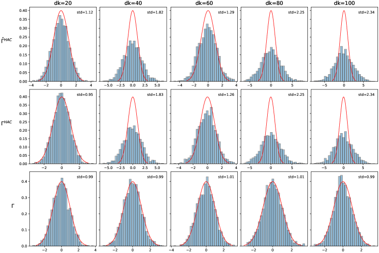
Figure 6: The histogram of the first entry of $\sqrt{d}\ \Sigma_{Be}^{-1/2}\left(\widehat{f}_{t}-f_{t}\right)$ for $t=0$, under $n=\sqrt{\min(d,T)}$ and $T=1000$. The first row shows the results for $\widehat{\Sigma}_{Be}=\widehat{\Gamma}^{HAC}$; the second row shows the results for $\widehat{\Sigma}_{Be}=\Gamma^{HAC}$; the third row shows the results for $\widehat{\Sigma}_{Be}=\Gamma$. Columns from left to right show the results for $d=20,40,60,80,100$. The sample standard deviation of the histograms are shown at the top right corner of each plot.

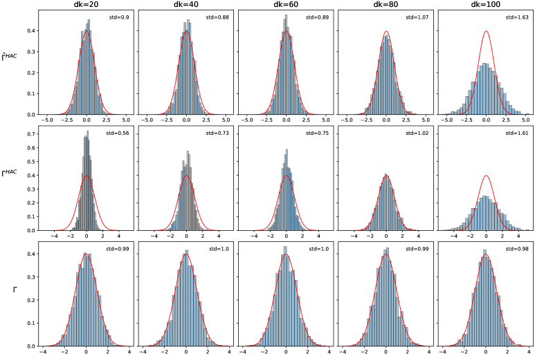
Figure 7: The histogram of the first entry of $\sqrt{d}\ \Sigma_{Be}^{-1/2}\left(\widehat{f}_{t}-f_{t}\right)$ for $t=0$, under $n=\lceil d^{3/4}\rceil$ and $T=500+\lceil d^{4/5}\rceil$. The first row shows the results for $\widehat{\Sigma}_{Be}=\widehat{\Gamma}^{HAC}$; the second row shows the results for $\widehat{\Sigma}_{Be}=\Gamma^{HAC}$; the third row shows the results for $\widehat{\Sigma}_{Be}=\Gamma$. Columns from left to right show the results for $d=20,40,60,80,100$. The sample standard deviation of the histograms are shown at the top right corner of each plot.

Appendix D: Consistency of the factor estimators

In this appendix, we show that CC-ISO requires a weaker condition for consistency of the factor estimators than PCA. Consider the model for data generating process in Appendix C, the specifications of the model are as follows:

• $d_{1}=d_{2}$, $r=3$ and $T=100+d^{0.3}$;

• Factor loadings are generated as in Section 5;

• $\rho_{1}=0.6,\rho_{2}=0.5,\rho_{3}=0.4$;

• $\Sigma_{{\cal E}_{k}}=Toeplitz(0.5,d_{k})$;

• $s_{i}=(r-i+1)\sqrt{d^{\alpha}}$, where $\alpha\in\{0.6,0.5,0.4\}$.

Under this data generating process, we have $\frac{1}{2}<\alpha+0.3<1$. As discussed in Remark 3.1, CC-ISO is consistent but PCA is not in theory. Figure 8 shows the estimation error of factors $\frac{1}{\sqrt{T}}\|\widehat{F}-HF\|_{2}$ for PCA and CC-ISO. It can be observed that PCA is not consistent for the factor estimation, while CC-ISO is consistent, which is in line with the theoretical results.

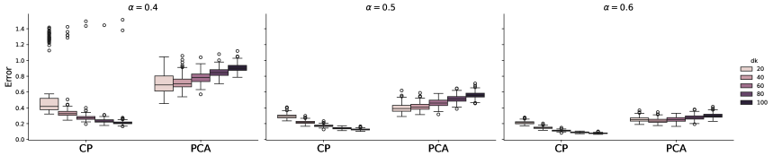
Figure 8: Factor estimation error for PCA and CC-ISO for different choices of $\alpha$ and $d_{k}$.

Appendix E: Further discussion of Assumption 3.1(ii)

The $\alpha$-mixing condition imposed in Assumption 3.1(ii) might not be flexible enough to accommodate some time series models (Andrews, (1984)). There are several ways to address this. One possibility is to impose higher-level assumptions, for example assuming directly a CLT and a probability limit, as in Bai, (2003) and Stock and Watson, (2002). Alternatively, we could adopt the more flexible $\tau$-mixing framework (see, Babii et al., (2024); Han and Wu, (2023)) or functional dependence measure (Wu,, 2005), which accomodates a broader class of time series processes. However, unlike $\alpha-$mixing, the $\tau-$mixing property is not preserved under measurable transformations, which complicates the analysis of quadratic or product terms. To deal with this, one can use truncation arguments in the proofs.

For instance, if we replace Assumption 3.1 (ii) with the assumption that $(f_{t})$ is $\tau-$mixing with mixing coefficient

$$\tau(m)\leq\exp\left(-c_{0}m^{\gamma}\right)$$ (60)

for some constants $c_{0}>0$ and $\gamma\geq 0$, then equation (40) in the appendix can still be established, albeit at a slightly slower rate. Specifically, we obtain the following lemma:

Lemma B.13.

Under the assumptions of Theorem 3.1 with the above $\tau-$mixing condition, we have

$$\frac{1}{T}\sum_{t=1}^{T}\!\big(\widetilde{f}_{it}^{2}-s_{it}^{2}\big)\;=\;s_{i}^{2}O_{p}\!\Big(\frac{(\log T)^{2/\nu_{2}}}{\sqrt{T}}\Big).$$

Proof.

Let $B_{T}=\;\Big(C\log T\Big)^{1/\nu_{2}}$ for some constant $C$. Define the truncated variable and the remainder

$$h_{it}=\min\{f_{it}^{2},B_{T}^{2}\},\qquad r_{it}=f_{it}^{2}-h_{it}=f_{it}^{2}\mathbf{1}\{|f_{it}|>B_{T}\}.$$

Then

$$\frac{1}{T}\sum_{t=1}^{T}\!\big(\widetilde{f}_{it}^{2}-\mathbb{E}\widetilde{f}_{it}^{2}\big)=\frac{1}{Ts_{i}^{2}}\sum_{t=1}^{T}\!\big(h_{it}-\mathbb{E}h_{it}\big)\;+\;\frac{1}{Ts_{i}^{2}}\sum_{t=1}^{T}\!\big(r_{it}-\mathbb{E}r_{it}\big).$$ (61)

For the first part in equation (61), set $\bar{h}_{it}=h_{it}-\mathbb{E}h_{it}$. We have $|\bar{h}_{it}|\leq B_{T}^{2}$ and $h_{it}$ is globally $2B_{T}$-Lipschitz. By the Lipschitz–$\tau$ covariance inequality, we have

$$V_{T}=Var(h_{it})+2\sum_{k\geq 1}|Cov(h_{it},h_{i,t+k})|=O(B_{T}^{4}).$$

Then by Bernstein inequality, we have for $\frac{1}{\gamma}=\frac{2}{\gamma_{1}}+\frac{1}{\gamma_{2}}$ $c_{1},c_{2}>0$,

$$\begin{split}P\left[Ts_{i}^{-2}\left(\frac{1}{T}\sum_{t=1}^{T}(h_{it}-\mathbb{E}h_{it})\geq\varepsilon\right)\right]\leq(T+1)\exp\!\Big(-c_{1}(T\varepsilon)^{\gamma}\Big)+&\exp\!\Big(-\,\frac{T^{2}\varepsilon^{2}}{c_{2}\,[1+TV_{T}]}\Big).\\ \end{split}$$

Let $\varepsilon=C\frac{B_{T}^{2}}{\sqrt{T}}$. It is easy to check the first exponential term vanishes to 0 and the second term is the dominating term. Note that

$$\exp\!\Big(-\,\frac{T^{2}\varepsilon^{2}}{c_{2}\,[1+TV_{T}]}\Big)\asymp\exp\left(-C^{2}/c_{2}\right).$$

Hence, for any $\delta>0$, we can always find $C$, so that

$$\begin{split}P\left[Ts_{i}^{-2}\left(\frac{1}{T}\sum_{t=1}^{T}(h_{it}-\mathbb{E}h_{it})\geq\varepsilon\right)\right]\leq\delta,\\ \end{split}$$

which implies that

$$\frac{1}{T}\sum_{t=1}^{T}(h_{it}-\mathbb{E}h_{it})=s_{i}^{2}O_{p}\!\Big(\frac{(\log T)^{2/\nu_{2}}}{\sqrt{T}}\Big).$$

For the second part of equation (61), we have

$$\mathbb{E}\,r_{it}=B_{T}^{2}P(|f_{t}|>B_{T})+\int_{B_{T}}^{\infty}2x\,P(|f_{it}|>x)\,dx\leq C^{\prime}(\log T)^{(2-\nu_{2})/\nu_{2}}\,T^{-c_{2}C}$$

by Assumption 3.1(ii). Therefore, by Markov’s inequality,

$$P\!\left(\frac{1}{T}\sum_{t=1}^{T}r_{it}>(\log T)^{2/\nu_{2}}/\sqrt{T}\right)\;\leq\;\frac{\mathbb{E}r_{it}}{(\log T)^{2/\nu_{2}}/\sqrt{T}}\;=\;O\!\big((\log T)^{-1}T^{-c_{2}C+1/2}\big)\to 0$$

for large $C$. Moreover,

$$\left|\frac{1}{T}\sum_{t=1}^{T}\!\big(r_{it}-\mathbb{E}r_{it}\big)\right|\;\leq\;\frac{1}{T}\sum_{t=1}^{T}r_{it}+\mathbb{E}r_{it}\;=\;o_{p}\!\Big(\frac{(\log T)^{2/\nu_{2}}}{\sqrt{T}}\Big).$$

Finally, combining two parts, we have

$$\frac{1}{T}\sum_{t=1}^{T}\!\big(\widetilde{f}_{it}^{2}-s_{it}^{2}\big)\;=\;s_{i}^{2}O_{p}\!\Big(\frac{(\log T)^{2/\nu_{2}}}{\sqrt{T}}\Big).$$

∎

Similar arguments can be used if we replace Assumptions 3.4 and 4.1(ii) with a $\tau$-mixing condition on $R_{t}=(f_{t}^{\top},z_{t}^{\top},e_{t}^{\top},\varepsilon_{t}^{\top},V_{t}^{\top})^{\top}$. In that case, truncated products such as $z_{t}e_{t}$, $e_{t}\varepsilon_{t}$, and $f_{t}\varepsilon_{t}$ can be bounded with Bernstein’s inequality, and the corresponding tail terms remain negligible.

We emphasize that these modifications are technically feasible but considerably increase the complexity of the proofs, which are already heavy. For this reason, we chose to work with $\alpha$-mixing in the main text and only provide a discussion of the $\tau$-mixing alternative in the appendix. Importantly, our simulation study confirms that the proposed method is robust to AR(1) dynamics, lending further support to the practical relevance of our assumptions.

Appendix F: Constructing Prediction Intervals under Post-Selection Debiased LASSO

This appendix outlines a practical procedure for constructing prediction intervals for $\widehat{y}_{T+h|T}$ using the post-selection debiased LASSO (PD-LASSO).

Step 1. Estimate latent factors.

Obtain factor estimates $\widehat{f}_{t}$ and loadings $\widehat{B}$ using the CC-ISO algorithm.

Step 2. Obtain projected residuals.

Regress $w_{t}$ on $\widehat{f}_{t}$ to remove the factor component:

$$\widehat{\Lambda}=\Big(\sum_{t=1}^{T}w_{t}\widehat{f}_{t}^{\prime}\Big)\Big(\sum_{t=1}^{T}\widehat{f}_{t}\widehat{f}_{t}^{\prime}\Big)^{-1},\qquad\widehat{V}_{t}=w_{t}-\widehat{\Lambda}\widehat{f}_{t}.$$

Then regress $y_{t+h}$ on $\widehat{f}_{t}$ to obtain the projection residuals:

$$\widetilde{y}_{t+h}=y_{t+h}-\widehat{\beta}_{1}^{*\top}\widehat{f}_{t},\qquad\widehat{\beta}_{1}^{*}=\Big(\sum_{t=1}^{T-h}\widehat{f}_{t}\widehat{f}_{t}^{\prime}\Big)^{-1}\Big(\sum_{t=1}^{T-h}\widehat{f}_{t}y_{t+h}\Big).$$

Step 3. LASSO estimation.

Estimate the local-predictor coefficients by

$$\widehat{\beta}_{0}=\arg\min_{\beta_{0}}\tfrac{1}{2T}\|\widetilde{Y}-\widehat{V}\beta_{0}\|_{2}^{2}+\lambda\|\beta_{0}\|_{1},$$

and define the selected support $\widehat{\mathcal{S}}=\{j:\widehat{\beta}_{0,j}\neq 0\}$.

Step 4. Nodewise precision estimation.

For each $j\in\widehat{\mathcal{S}}$, estimate the $j$th row of the precision matrix via

$$\widehat{\gamma}_{j}=\arg\min_{\gamma_{j}}\tfrac{1}{T}\|\widehat{V}_{j}-\widehat{V}_{-j}\gamma_{j}\|_{2}^{2}+\lambda_{j}\|\gamma_{j}\|_{1},\qquad\widehat{\tau}_{j}^{2}=\tfrac{1}{T}\|\widehat{V}_{j}-\widehat{V}_{-j}\widehat{\gamma}_{j}\|_{2}^{2}+\lambda_{j}\|\widehat{\gamma}_{j}\|_{1}.$$

Assemble $\widehat{\Gamma}_{\widehat{\mathcal{S}}}$ and $\mathbf{T}_{\widehat{\mathcal{S}}}$ (diagonal with entries $\widehat{\tau}_{j}^{-2}$), and set $\widehat{\Theta}_{\widehat{\mathcal{S}}}=\mathbf{T}_{\widehat{\mathcal{S}}}\widehat{\Gamma}_{\widehat{\mathcal{S}}}$.

Step 5. Post-selection debiasing.

Compute

$$\widehat{\beta}_{0}^{(PL)}=\widehat{\beta}_{0}+\tfrac{1}{T}\widehat{\Theta}_{\widehat{\mathcal{S}}}\widehat{V}(\widetilde{Y}-\widehat{V}\widehat{\beta}_{0}).$$

Re-estimate $\beta_{1}$ and residuals:

$$\widehat{\beta}_{1}=(\widehat{F}^{\prime}\widehat{F})^{-1}\widehat{F}(Y-W\widehat{\beta}_{0}^{(PL)}),\qquad\widehat{\varepsilon}=Y-W\widehat{\beta}_{0}^{(PL)}-\widehat{F}\widehat{\beta}_{1}.$$

Step 6. Forecast and variance estimation.

Compute the forecast $\widehat{y}_{T+h|T}=w_{T}^{\prime}\widehat{\beta}_{0}^{(PL)}+\widehat{f}_{T}^{\prime}\widehat{\beta}_{1}$ and its variance

$$\widehat{\sigma}_{\widehat{y}_{T+h|T}}=\widehat{\sigma}_{y,\widehat{\beta}_{0}}+\widehat{\sigma}_{y,\widehat{\beta}_{1}}+\widehat{\sigma}_{\widehat{f}_{T}},$$

where

$$\widehat{\sigma}_{y,\widehat{\beta}_{1}} =\tfrac{1}{T}\widehat{f}_{T}^{\prime}\Big(\tfrac{1}{T}\sum_{t=1}^{T-h}\widehat{f}_{t}\widehat{f}_{t}^{\prime}\Big)^{-1}\Big(\tfrac{1}{T}\sum_{t=1}^{T-h}\widehat{f}_{t}\widehat{f}_{t}^{\prime}\widehat{\varepsilon}_{t+h}^{2}\Big)\widehat{f}_{T},$$

$$\widehat{\sigma}_{\widehat{f}_{T}} =\widehat{\beta}_{1}^{\prime}\widehat{S}^{-1}\widehat{B}^{\prime}\widehat{\Sigma}_{Be}\widehat{B}\widehat{S}^{-1}\widehat{\beta}_{1},$$

$$\widehat{\sigma}_{y,\widehat{\beta}_{0}} =\tfrac{1}{T}\widehat{V}_{T}^{\prime}\widehat{\Theta}_{\widehat{\mathcal{S}}}\widehat{\Omega}\widehat{\Theta}_{\widehat{\mathcal{S}}}\widehat{V}_{T},$$

with $\widehat{\Sigma}_{Be}$ and $\widehat{\Omega}$ obtained via the thresholding estimators defined in Section 3.3.

Step 7. Construct the prediction interval.

The $(1-\alpha)\%$ prediction interval is

$$\Big[\widehat{y}_{T+h|T}-q_{\alpha/2}\widehat{\sigma}_{\widehat{y}_{T+h|T}},\,\widehat{y}_{T+h|T}+q_{\alpha/2}\widehat{\sigma}_{\widehat{y}_{T+h|T}}\Big],$$

where $q_{\alpha/2}$ is the upper $\alpha/2$ quantile of the standard normal distribution.

This PD-LASSO procedure offers a practical approach for constructing approximate prediction intervals in high-dimensional forecasting. Our simulation study suggests that PD-LASSO intervals achieve coverage rates close to nominal levels while remaining narrower than those from the fully debiased LASSO, providing a useful balance between validity and efficiency.

We conduct a simulation study to evaluate its performance. The DGP mainly follows Section 5.4 with minor modifications:

• $p=100$ and $d_{k}\in\{40,80,100\}$. $T=800+\lceil d^{3/4}\rceil$.

• $V_{t}$ is generated independently from $N(0,\Sigma_{V})$ where $\Sigma_{V}=Toeplitz(0.5,p)$.

• Factor strength $\alpha_{i}=\alpha\in\{1,0.6,0.4\}$.

• $\beta_{0}=(3,3,3,0,\ldots,0)^{\prime}$.

The tuning parameter $\lambda$ is the Step 3 is selected through BIC and $\lambda_{j}$ in Step 4 are fixed at $\sqrt{\log(d)/T}+\sqrt{1/\widehat{s}_{r}}$ for all $j$.

Table 4 reports the results. Coverage rates of the proposed PD-LASSO are close to the nominal 95% level. The close coverage rate of PD-LASSO is mainly due to the high variable-selection accuracy achieved by BIC. These findings suggest that PD-LASSO offers a useful compromise, which provides approximately valid coverage with narrower intervals when the selection step is reliable.

Table 4: Results of prediction intervals post-selection debiased LASSO

	$\alpha=1$		$\alpha=0.6$		$\alpha=0.4$
$d_{k}$	PI Length	Coverage Rate	PI Length	Coverage Rate	PI Length	Coverage Rate
40	0.369	0.913	0.784	0.905	1.294	0.858
80	0.286	0.935	0.589	0.919	1.137	0.883
100	0.257	0.934	0.503	0.927	1.062	0.92

Appendix G: More simulation results

In this section, we conduct additional simulation studies. Firstly, we check the robustness of our proposed algorithm under (i) more persistent factors, (ii) stronger cross-sectional correlation in errors, and (iii) Student-t errors. For all DGP settings, we evaluate the coverage rate of prediction intervals in the low-dimensional $w_{t}$ setting and the forecast errors for MS-FASR in the high-dimensional $w_{t}$ setting. Throughout, we fix $\alpha_{i}=\alpha=0.6$ and $d_{k}=40$.

To generate more persistent factors, we specify:

$$g_{i,t+1}=\rho g_{i,t}+\sqrt{1-\rho^{2}}u_{it},\quad\rho\in\{0.7,0.8,0.9\}$$

$$f_{t}=\Sigma_{f}^{1/2}g_{t}$$

where $u_{it}$ is generated independently from standard normal and $\Sigma_{f}=Toeplitz(0.5,r)$ inducing correlation among factors. Other settings follow Section 5 of the main text.

To allow stronger error dependence, we vary $\kappa\in\{0.6,0.7,0.8\}$ in $\Sigma_{{\cal E},1}=\Sigma_{{\cal E},2}=Toeplitz(\kappa,d_{k}),$ thereby varying the level of dependence. The remaining settings are the same as in Section 5.

For the Student-t errors design, we generate ${\cal E}_{t}$ as follows:

$${\cal E}_{t}=\Sigma_{{\cal E},1}^{1/2}Z_{t}\Sigma_{{\cal E},2}^{1/2},\quad\Sigma_{{\cal E},1}=\Sigma_{{\cal E},2}=Toeplitz(0.5,d_{k}),$$

where each entry of $Z_{t}$ is drawn independently from student-t distribution with degrees of freedom $df\in\{4,5,6\}$. The regression error $\epsilon_{t+h}$ is generated from the same distribution. Other settings again follow Section 5.

The prediction errors of MS-FASR are reported in Figure 9, 10 and 11, while the coverage rates of CP and PCA prediction intervals in the low-dimensional regressor setting are presented in Table 5. The results show that our method remains robust and performs well across these alternative designs.

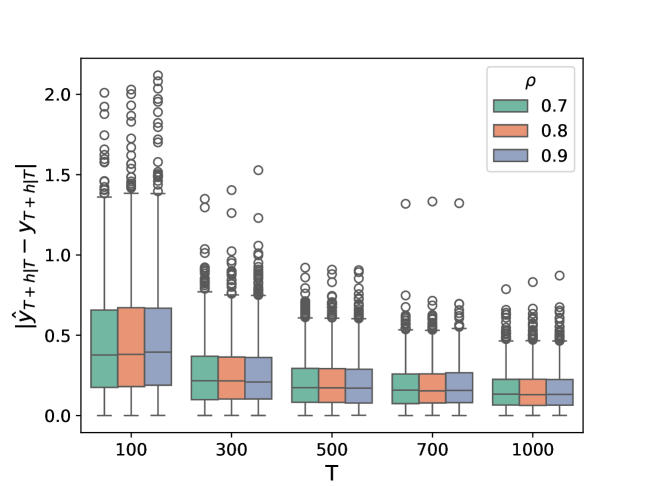
Figure 9: Boxplots of prediction errors $|\widehat{y}_{T+h|T}-y_{T+h|T}|$ of MS-FASR under more persistent factors.

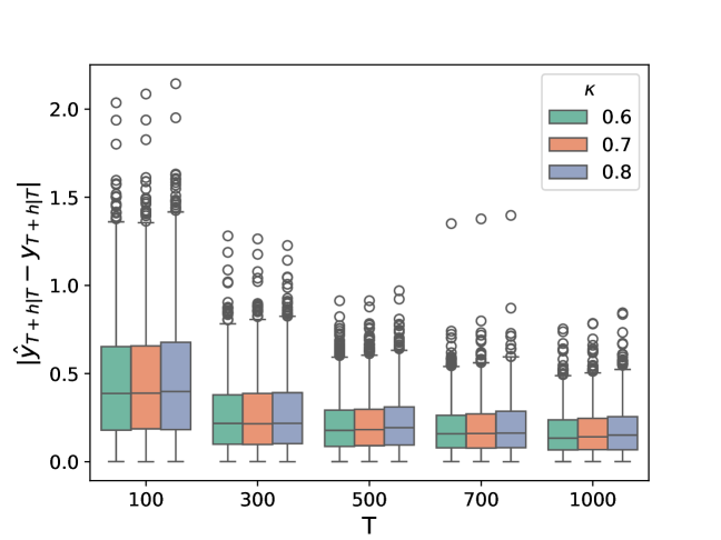
Figure 10: Boxplots of prediction errors $|\widehat{y}_{T+h|T}-y_{T+h|T}|$ of MS-FASR under stronger error dependence in CP factor model.

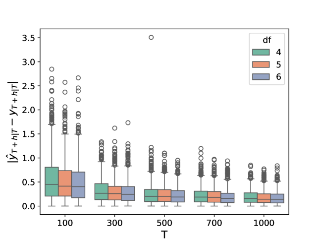
Figure 11: Boxplots of prediction errors $|\widehat{y}_{T+h|T}-y_{T+h|T}|$ of MS-FASR under student-t distributions.

Table 5: Coverage rate of CP and PCA prediction intervals

	CP	PCA(H)	PCA(T)
Persistent factors
$\rho$
0.7	0.94	0.73	0.753
0.8	0.942	0.724	0.753
0.9	0.947	0.737	0.765
Stronger error dependence
$\kappa$
0.6	0.936	0.703	0.739
0.7	0.933	0.642	0.689
0.8	0.915	0.47	0.527
Student t errors
$df$
4	0.917	0.72	0.743
5	0.917	0.719	0.739
6	0.929	0.731	0.759

Note: (1) The dimension $d_{k}$ and the factor signal $\alpha$ are fixed at 40 and 0.6, respectively. (2) PCA(T) and PCA(H) refer to the prediction interval constructed using the PCA approach, where the covariance matrix of the factors is estimated via the proposed thresholding covariance estimator and the HAC-type estimator proposed by Bai and Ng, (2006) and Bai and Ng, (2023), respectively. (3) The nominal confidence level is $95\%$.

Next, we evaluate the convergence rate in Theorem 3.1 by a simulation study in which the factors are generated independently from standard normal distributions, while all other settings follow Section 5. Under this DGP setting, the theoretical rate for $\|\widehat{f_{T}}-Hf_{T}\|_{2}$ is $\sqrt{\frac{1}{d^{\alpha-1/2}T}}+\frac{1}{d^{\alpha/2}}$. We fix $T=500$, $\alpha=0.6$ and let $d_{1}=d_{2}=\bar{d}$ with increasing $\bar{d}$. Figure 13 shows the comparison between the simulated and the theoretical rates of factor estimation, showing that the simulation curve closely aligns with the theoretical curve.

Finally, we conducted an additional simulation to evaluate the performance of MS-FASR when $w_{t}$ is generated independently of $f_{t}$ (i.e., $\Lambda=0$). The DGP follows Section 5.4 in the paper with $\alpha=0.6$, $d_{k}=40$ and $T\in\{100,300,500,700,1000\}$. Figure 12 shows the boxplots of the estimations error $\|\widehat{\beta}_{0}-\beta_{0}\|_{1}$ and forecast error $|\widehat{y}_{T+h|T}-y_{T+h|T}|$. The results show that the independence between $w_{t}$ and $f_{t}$ does not affect the performance of our algorithm, confirming its robustness to the absence of shared latent structure. See the discussion on Page 21.

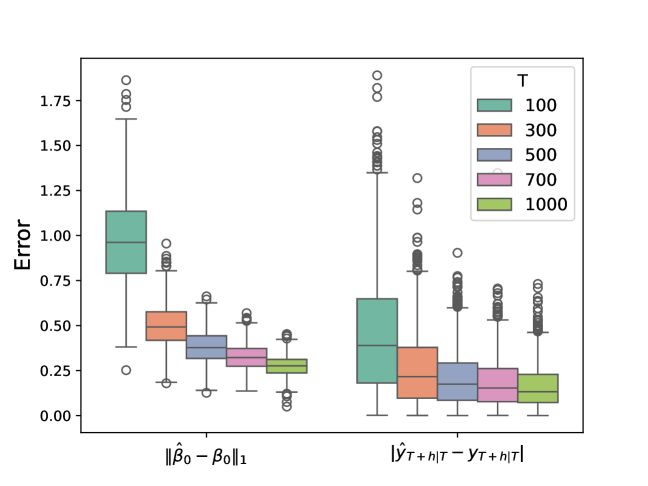
Figure 12: Boxplots of errors for MS-FASR where $W$ is not related to $F$.

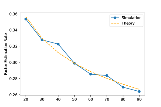
Figure 13: Simulated rates vs. theoretical rates of factor estimation. The blue solid lines show the mean of simulated estimation errors over 200 repetitions. The orange dotted lines show the fitted curve of theoretical rates. The fitted curve is $c_{0}\sqrt{\frac{1}{d^{0.1}T}}+c_{1}\frac{1}{d^{0.3}}$ where $c_{0}$ and $c_{1}$ are calculated by minimizing the distance between the theoretical curve and the simulation curve.

References

- Adamek et al., (2023) Adamek, R., Smeekes, S., and Wilms, I. (2023). Lasso inference for high-dimensional time series. Journal of econometrics, 235(2):1114–1143.
- Ahn and Horenstein, (2013) Ahn, S. C. and Horenstein, A. R. (2013). Eigenvalue ratio test for the number of factors. Econometrica, 81(3):1203–1227.
- Andrews, (1984) Andrews, D. W. K. (1984). Non-strong mixing autoregressive processes. Journal of Applied Probability, 21(4):930–934.
- Babii et al., (2023) Babii, A., Ghysels, E., and Pan, J. (2023). Tensor principal component analysis. Working paper.
- Babii et al., (2025) Babii, A., Ghysels, E., and Pan, J. (2025). Tensor principal component analysis. arXiv preprint arXiv:2212.12981.
- Babii et al., (2022) Babii, A., Ghysels, E., and Striaukas, J. (2022). Machine learning time series regressions with an application to nowcasting. Journal of Business & Economic Statistics, 40(3):1094–1106.
- Babii et al., (2024) Babii, A., Ghysels, E., and Striaukas, J. (2024). High-dimensional granger causality tests with an application to vix and news. Journal of Financial Econometrics, 22(3):605–635.
- Bai, (2003) Bai, J. (2003). Inferential theory for factor models of large dimensions. Econometrica, 71(1):135–171.
- Bai and Ng, (2006) Bai, J. and Ng, S. (2006). Confidence intervals for diffusion index forecasts and inference for factor-augmented regressions. Econometrica, 74(4):1133–1150.
- Bai and Ng, (2023) Bai, J. and Ng, S. (2023). Approximate factor models with weaker loadings. Journal of Econometrics, 235(2):1893–1916.
- Beyhum, (2024) Beyhum, J. (2024). Factor-augmented sparse midas regressions with an application to nowcasting. Technical report, FEB Research Report, Department of Economics.
- Beyhum and Gautier, (2022) Beyhum, J. and Gautier, E. (2022). Factor and factor loading augmented estimators for panel regression with possibly nonstrong factors. Journal of Business & Economic Statistics, 41(1):270–281.
- Bickel and Levina, (2008) Bickel, P. J. and Levina, E. (2008). Covariance regularization by thresholding. The Annals of Statistics, 36(6):2577 – 2604.
- Bühlmann and Van De Geer, (2011) Bühlmann, P. and Van De Geer, S. (2011). Statistics for high-dimensional data: methods, theory and applications. Springer Science & Business Media.
- Bussiere et al., (2009) Bussiere, M., Chudik, A., and Sestieri, G. (2009). Modelling global trade flows: Results from a gvar model. ECB Working Paper No. 1087. Available at SSRN: https://ssrn.com/abstract=1456883 or http://dx.doi.org/10.2139/ssrn.1456883.
- Cai and Liu, (2011) Cai, T. and Liu, W. (2011). Adaptive thresholding for sparse covariance matrix estimation. Journal of the American Statistical Association, 106(494):672–684.
- Cai et al., (2025) Cai, X., Kong, X., Wu, X., and Zhao, P. (2025). Matrix-factor-augmented regression. Journal of Business & Economic Statistics, pages 1–13.
- (18) Chen, B., Han, Y., and Yu, Q. (2024a). Estimation and inference for cp tensor factor models. arXiv preprint arXiv:2406.17278.
- Chen and Fan, (2023) Chen, E. Y. and Fan, J. (2023). Statistical inference for high-dimensional matrix-variate factor models. Journal of the American Statistical Association, 118(542):1038–1055.
- (20) Chen, E. Y., Fan, J., and Zhu, X. (2024b). Factor augmented matrix regression. Working paper, Princeton University.
- Chen et al., (2012) Chen, J., Gao, J., and Li, D. (2012). Semiparametric trending panel data models with cross-sectional dependence. Journal of Econometrics, 171(1):71–85.
- Chernozhukov et al., (2018) Chernozhukov, V., Chetverikov, D., Demirer, M., Duflo, E., Hansen, C., Newey, W., and Robins, J. (2018). Double/debiased machine learning for treatment and structural parameters. The Econometrics Journal, 21(1):C1–C68.
- Chernozhukov et al., (2021) Chernozhukov, V., Härdle, W. K., Huang, C., and Wang, W. (2021). Lasso-driven inference in time and space. The Annals of Statistics, 49(3):1702–1735.
- den Haan and Levin, (1997) den Haan, W. J. and Levin, A. T. (1997). A practitioner’s guide to robust covariance matrix estimation. In Robust Inference, volume 15 of Handbook of Statistics, pages 299–342. Elsevier.
- Diebold and Mariano, (1995) Diebold, F. X. and Mariano, R. S. (1995). Comparing predictive accuracy. Journal of Business and Economic Statistics, 13(3):253–263.
- Fan and Li, (2001) Fan, J. and Li, R. (2001). Variable selection via nonconcave penalized likelihood and its oracle properties. Journal of the American Statistical Association, 96(456):1348–1360.
- Fan et al., (2011) Fan, J., Liao, Y., and Mincheva, M. (2011). High-dimensional covariance matrix estimation in approximate factor models. The Annals of statistics, 39(6):3320–3356.
- Fan et al., (2013) Fan, J., Liao, Y., and Mincheva, M. (2013). Large covariance estimation by thresholding principal orthogonal complements. Journal of the Royal Statistical Society. Series B, Statistical methodology, 75(4):603–680.
- Fan et al., (2024) Fan, J., Lou, Z., and Yu, M. (2024). Are latent factor regression and sparse regression adequate? Journal of the American Statistical Association, 119(546):1076–1088.
- Gao and Tsay, (2024) Gao, Z. and Tsay, R. S. (2024). Supervised dynamic pca: Linear dynamic forecasting with many predictors. Journal of the American Statistical Association, pages 1–15.
- Gonçalves and Perron, (2014) Gonçalves, S. and Perron, B. (2014). Bootstrapping factor-augmented regression models. Journal of Econometrics, 182(1):156–173. Causality, Prediction, and Specification Analysis: Recent Advances and Future Directions.
- Greenwood-Nimmo et al., (2012) Greenwood-Nimmo, M., Nguyen, V., and Shin, Y. (2012). Probabilistic forecasting of output, growth, inflation and the balance of trade in a gvar framework. Journal of Applied Econometrics, pages 554–573.
- Han et al., (2015) Han, F., Lu, H., and Liu, H. (2015). A direct estimation of high dimensional stationary vector autoregressions. J. Mach. Learn. Res., 16(1):3115–3150.
- Han and Wu, (2023) Han, F. and Wu, W. B. (2023). Probability inequalities for high-dimensional time series under a triangular array framework. In Springer Handbook of Engineering Statistics, pages 849–863. Springer.
- Han et al., (2024) Han, Y., Yang, D., Zhang, C.-H., and Chen, R. (2024). Cp factor model for dynamic tensors. Journal of the Royal Statistical Society Series B: Statistical Methodology, 86(5):1383–1413.
- Huang et al., (2022) Huang, D., Jiang, F., Li, K., Tong, G., and Zhou, G. (2022). Scaled pca: A new approach to dimension reduction. Management Science, 68(3):1678–1695.
- Jurado et al., (2015) Jurado, K., Ludvigson, S. C., and Ng, S. (2015). Measuring uncertainty. American Economic Review, 105(3):1177–1216.
- Kiefer et al., (2000) Kiefer, N. M., Vogelsang, T. J., and Bunzel, H. (2000). Simple robust testing of regression hypotheses. Econometrica, 68(3):695–714.
- Kock and Callot, (2015) Kock, A. B. and Callot, L. (2015). Oracle inequalities for high dimensional vector autoregressions. Journal of Econometrics, 186(2):325–344. High Dimensional Problems in Econometrics.
- Kolda and Bader, (2009) Kolda, T. G. and Bader, B. W. (2009). Tensor decompositions and applications. SIAM Review, 51(3):455–500.
- Kruskal, (1977) Kruskal, J. (1977). Three-way arrays: rank and uniqueness of trilinear decompositions, with application to arithmetic complexity and statistics. Linear Algebra and its Applications, 18:95–138.
- Kruskal, (1989) Kruskal, J. (1989). Rank, decomposition, and uniqueness for 3-way and n-way arrays. Multiway Data Analysis, pages 7–18.
- Lam and Yao, (2012) Lam, C. and Yao, Q. (2012). Factor modeling for high-dimensional time series: inference for the number of factors. The Annals of Statistics, 40(2):694–726.
- Lee et al., (2016) Lee, J. D., Sun, D. L., Sun, Y., and Taylor, J. E. (2016). Exact post-selection inference, with application to the lasso. Annals of Statistics, 44(3):907–927.
- Liu et al., (2018) Liu, K., Markovic, J., and Tibshirani, R. (2018). More powerful post-selection inference, with application to the lasso. arXiv preprint arXiv:1801.09037.
- Loh and Wainwright, (2012) Loh, P.-L. and Wainwright, M. J. (2012). High-dimensional regression with noisy and missing data: Provable guarantees with nonconvexity. The Annals of statistics, 40(3):1637–1664.
- Ludvigson and Ng, (2007) Ludvigson, S. C. and Ng, S. (2007). The empirical risk-return relation: A factor analysis approach. Journal of Financial Economics, 83(1):171–222.
- Ludvigson and Ng, (2009) Ludvigson, S. C. and Ng, S. (2009). Macro factors in bond risk premia. The Review of Financial Studies, 22(12):5027–5067.
- McCracken and Ng, (2016) McCracken, M. W. and Ng, S. (2016). Fred-md: A monthly database for macroeconomic research. Journal of Business & Economic Statistics, 34(4):574–589.
- Medeiros and Mendes, (2016) Medeiros, M. C. and Mendes, E. F. (2016). 1-regularization of high-dimensional time-series models with non-gaussian and heteroskedastic errors. Journal of Econometrics, 191(1):255–271.
- Merlevède et al., (2011) Merlevède, F., Peligrad, M., and Rio, E. (2011). A bernstein type inequality and moderate deviations for weakly dependent sequences. Probability Theory and Related Fields, 151(3-4):435–474.
- Rothman et al., (2009) Rothman, A. J., Levina, E., and Zhu, J. (2009). Generalized thresholding of large covariance matrices. Journal of the American Statistical Association, 104(485):177–186.
- Shapley, (1953) Shapley, L. (1953). A value for n-person games. Contributions to the theory of games, 2:307–317.
- Sidiropoulos and Bro, (2000) Sidiropoulos, N. and Bro, R. (2000). On the uniqueness of multilinear decomposition of n-way arrays. Journal of Chemometrics, 14:229–239.
- Song and Bickel, (2011) Song, S. and Bickel, P. J. (2011). Large vector auto regressions. arXiv preprint arXiv:1106.3915.
- Stock and Watson, (2002) Stock, J. H. and Watson, M. W. (2002). Macroeconomic forecasting using diffusion indexes. Journal of Business & Economic Statistics, 20(2):147–162.
- Vershynin, (2024) Vershynin, R. (2024). High-Dimensional Probability: An Introduction with Applications in Data Science. Cambridge University Press.
- Wu, (2005) Wu, W. B. (2005). Nonlinear system theory: Another look at dependence. Proceedings of the National Academy of Sciences, 102(40):14150–14154.
- Xia, (2021) Xia, D. (2021). Normal approximation and confidence region of singular subspaces. Electronic journal of statistics, 15(2):3798–3851.