On Eigenvector Computation and Eigenvalue Reordering for the Non-Hermitian Quaternion Eigenvalue Problem

Abstract

In this paper we present several additions to the quaternion QR algorithm, including algorithms for eigenvector computation and eigenvalue reordering. A key outcome of the eigenvalue reordering algorithm is that the aggressive early deflation (AED) technique, which significantly enhances the convergence of the QR algorithm, is successfully applied to the quaternion eigenvalue problem. We conduct numerical experiments to demonstrate the efficiency and effectiveness of the proposed algorithms.

Keywords: Non-Hermitian eigenvalue problem, quaternion QR algorithm, eigenvector, eigenvalue reordering, aggressive early deflation

MSC code (2020). 65F15, 15A33, 15A18

1 Introduction

Let $\mathbb{H}=\operatorname{span}_{\mathbb{R}}\left\{1,\mathrm{i},\mathrm{j},\mathrm{k}\right\}$ be the skew field of quaternions, where the basis satisfies

$$\mathrm{i}^{2}=\mathrm{j}^{2}=\mathrm{k}^{2}=\mathrm{i}\mathrm{j}\mathrm{k}=-1.$$

The quaternion (right) eigenvalue problem

$$\bm{A}\bm{x}=\bm{x}\lambda,\qquad(\bm{A}\in\mathbb{H}^{n\times n},~\bm{x}\in\mathbb{H}^{n}\setminus\left\{0\right\},~\lambda\in\mathbb{H})$$

arises in a variety of applications, including quantum mechanics [1, 18], image processing [25, 26], etc. In this work, we restrict ourselves to the dense, non-Hermitian case (i.e., the matrix $\bm{A}$ is a dense, non-Hermitian quaternion matrix). The non-Hermitian quaternion eigenvalue problem naturally emerges in non-Hermitian quantum mechanics [18].

The dense non-Hermitian quaternion eigenvalue problem has been studied in [7, 16]. In [7] the (nonsymmetric) Francis QR algorithm [9, 10] was successfully extended to compute the quaternion Schur decomposition. Recently the quaternion QR algorithm was reformulated into a structure-preserving manner in order to improve performance [16]. However, a few closely related computational tasks, such as eigenvector computation and eigenvalue reordering, are not discussed in these works. Moreover, in the past decades, the Francis QR algorithm has been largely improved by modern techniques such as multishift QR sweeps and aggressive early deflation (AED) [3, 4, 5, 8, 14, 15, 19]. These modern techniques have not yet been incorporated into the quaternion QR algorithm.

In this work we discuss several aspects in the dense, non-Hermitian quaternion eigenvalue problem that have not been carefully addressed in the existing literature. We first establish tools to effectively solve upper triangular quaternion Sylvester equations. Then the quaternion Sylvester solvers are adopted to tackle higher level problems, including the computation of all or selected eigenvectors, the eigenvalue swapping problem, as well as the application of the AED technique. Thanks to these developments, we obtain a dense, non-Hermitian quaternion eigensolver that is more efficient and complete.

This paper is an extension of the undergraduate thesis of the third author [30]. The rest of the paper is organized as follows. In Section 2, we briefly review some basics of the quaternion (right) eigenvalue problem. In Section 3, we discuss quaternion Sylvester equation solvers and develop algorithms for eigenvector computation for upper triangular quaternion matrices. In Section 4, we propose the eigenvalue swapping algorithm and develop the AED technique. Numerical experiments are presented in Section 5.

2 Quaternion right eigenvalue problem

In the following we provide a brief review of the quaternion right eigenvalue problem. We assume that readers are already familiar with quaternion algebra.

Given a quaternion matrix $\bm{A}\in\mathbb{H}^{n\times n}$, the right eigenvalue problem is to find a scalar $\lambda\in\mathbb{H}$ and a vector $\bm{x}\in\mathbb{H}^{n}\setminus\left\{0\right\}$ such that $\bm{A}\bm{x}=\bm{x}\lambda$. Recall that any two quaternions $\xi$ and $\eta$ are similar to each other if there exists a unit quaternion $\omega$ such that $\eta=\overline{\omega}\xi\omega$. Let $\ldbrack\xi\rdbrack$ denote the set of quaternions similar to $\xi$, and let $\mathbb{C}_{+}$ denote the upper half-plane including the real axis. Then $\ldbrack\xi\rdbrack\cap\mathbb{C}_{+}$ contains a unique element, denoted by $\xi_{c}$; see, e.g., [33, Lemma 2.1]. If $\xi$ is an eigenvalue of $\bm{A}$, then so is any other element of $\ldbrack\xi\rdbrack$. We call $\xi_{c}$ a standard eigenvalue or a standardized eigenvalue of $\bm{A}$. Then every eigenvalue of $\bm{A}$ can be standardized. In the rest of this paper we assume that all eigenvalues are already standardized unless otherwise specified.

From a numerical perspective, if many or all eigenvalues of $\bm{A}$ are of interest, it is recommended to compute the Schur decomposition

$$\bm{A}=\bm{U}\bm{T}\bm{U}^{\mathsf{H}},$$ (1)

where $\bm{U}\in\mathbb{H}^{n\times n}$ is unitary and $\bm{T}\in\mathbb{H}^{n\times n}$ is upper triangular with diagonal entries chosen from $\mathbb{C}_{+}$ [6]. The computation of (1) can be accomplished by the quaternion QR algorithm [7]; see Algorithm 1.

Algorithm 1 Quaternion QR Algorithm

0: A quaternion matrix $\bm{A}\in\mathbb{H}^{n\times n}$.

0: A unitary matrix $\bm{U}$ and an upper triangular matrix $\bm{T}$ satisfying (1).

1: Reduce $\bm{A}$ to an Hessenberg matrix $\bm{H}_{0}$ using unitary similarity: $\bm{H}_{0}=\bm{U}^{\mathsf{H}}\bm{A}\bm{U}$.

2: while not converged do

3:  Generate the (real) shifting polynomial $p_{k}(\cdot)$ for $\bm{H}_{k}$.

4:  Update $\bm{H}_{k+1}\leftarrow\bm{Q}_{k}^{\mathsf{H}}\bm{H}_{k}\bm{Q}_{k}$ using an implicit QR sweep, where $\bm{Q}_{k}\bm{R}_{k}$ is the QR factorization of $p_{k}(\bm{H}_{k})$.

5:  Update $\bm{U}\leftarrow\bm{U}\cdot\bm{Q}_{k}$.

6: end while

7: Standardize the diagonal entries of $\bm{H}_{k}$, and set $\bm{T}\leftarrow\bm{H}_{k}$.

We would like to make two remarks here. First, we shall see in Section 3.1 that eigenvector computation is a non-trivial task due to the non-commutativity of quaternion algebra. In practice it is often required to compute a few or all eigenvectors of $\bm{A}$ after the Schur decomposition (1) is calculated. However, neither [7] nor [16] provided a detailed discussion of how this can be done. We shall discuss eigenvector computation in Section 3. Second, in theory, the diagonal entries of $\bm{T}$ can take any prescribed ordering. This can be easily shown by induction. In Section 4, we shall discuss how to reorder the diagonal entries in the Schur form in a numerically stable manner.

3 Eigenvector computation from the quaternion Schur form

3.1 Motivation

For a complex matrix $\bm{A}\in\mathbb{C}^{n\times n}$, if an eigenvalue of the matrix, $\lambda$, is known, the corresponding eigenvector $\bm{x}$ can be computed by solving the homogeneous linear equation

$$(\bm{A}-\lambda\bm{I})\bm{x}=\bm{0}.$$ (2)

Since the coefficient matrix $\bm{A}-\lambda\bm{I}$ is singular, we usually impose an additional normalization assumption on $\bm{x}$, e.g., $\bm{x}(1)=1$, to ensure that the system (2) has a unique solution, if $\lambda$ is of multiplicity one.

The situation becomes more complicated for quaternion matrices. Let us assume that $\bm{A}\in\mathbb{H}^{n\times n}$ has a known single eigenvalue $\lambda\in\mathbb{C}_{+}$. Due to the non-commutativity of quaternion algebra, we need adjust (2) to a homogeneous Sylvester equation

$$\bm{A}\bm{x}-\bm{x}\lambda=\bm{0}.$$ (3)

However, there is a new obstacle that in general we cannot impose $\bm{x}(i)=1$ for any $i$, even if we can already ensure $\bm{x}(i)\neq 0$. Therefore, equation (3) is much more difficult to solve compared to (2).

For instance, consider

$$\bm{A}=\begin{bmatrix}2-\mathrm{i}-2\mathrm{j}&-1+\mathrm{i}+2\mathrm{j}\\ 2-2\mathrm{i}-2\mathrm{j}&-1+2\mathrm{i}+2\mathrm{j}\end{bmatrix}.$$

The eigenvalues of $\bm{A}$ are $\lambda_{1}=1$ and $\lambda_{2}=\mathrm{i}$, with eigenvectors

$$\bm{x}_{1}=\begin{bmatrix}1\\ 1\end{bmatrix},\qquad\bm{x}_{2}=\begin{bmatrix}1-\mathrm{j}+\mathrm{k}\\ 2-\mathrm{j}+\mathrm{k}\end{bmatrix}.$$

It is impossible to normalize any entry of $\bm{x}_{2}$ to $1$ or any other complex number, unless $\lambda_{2}$ is allowed to be replaced by a non-complex one in $\ldbrack\lambda_{2}\rdbrack$. Without the knowledge of $\bm{x}_{2}$, it is even unclear how to properly choose an element from $\ldbrack\lambda_{2}\rdbrack$ to make (3) easy to solve.

However, the situation becomes much simpler when $\bm{A}$ is in the Schur form. In the following, we shall show that the eigenvectors of an upper triangular quaternion matrix can be easily computed without augmenting the matrix dimension.

3.2 Upper triangular Sylvester equations

We first discuss how to solve upper triangular Sylvester equations that frequently arise in quaternion eigenvalue problems. The simplest case is the scalar Sylvester equation. Lemma 1 characterizes the nondegenerate case. Although this result is well-known, we provide here a constructive proof that is suitable for numerical computation.

Lemma 1 ([17]).

Let $\alpha$, $\beta$, $\gamma\in\mathbb{H}$. Then there exists a unique $\chi\in\mathbb{H}$ such that $\alpha\chi-\chi\beta=\gamma$ if and only if $\ldbrack\alpha\rdbrack\neq\ldbrack\beta\rdbrack$.

Proof.

Let $\xi_{1}$ and $\xi_{2}$ be unit quaternions such that $\tilde{\alpha}=\overline{\xi}_{1}\alpha\xi_{1}\in\mathbb{C}_{+}$ and $\tilde{\beta}=\overline{\xi}_{2}\beta\xi_{2}\in\mathbb{C}_{+}$. Then the Sylvester equation $\alpha\chi-\chi\beta=\gamma$ reduces to

$$\tilde{\alpha}\tilde{\chi}-\tilde{\chi}\tilde{\beta}=\tilde{\gamma},$$ (4)

where $\tilde{\chi}=\overline{\xi}_{1}\chi\xi_{2}$ and $\tilde{\gamma}=\overline{\xi}_{1}\gamma\xi_{2}$. By representing $\tilde{\chi}$ and $\tilde{\gamma}$, respectively, as

$$\tilde{\chi}=\tilde{\chi}_{1}+\tilde{\chi}_{2}\mathrm{j},\qquad\tilde{\gamma}=\tilde{\gamma}_{1}+\tilde{\gamma}_{2}\mathrm{j},\qquad(\tilde{\chi}_{1},\,\tilde{\chi}_{2},\,\tilde{\gamma}_{1},\,\tilde{\gamma}_{2}\in\mathbb{C}),$$

equation (4) splits into

$$(\tilde{\alpha}-\tilde{\beta})\tilde{\chi}_{1}=\tilde{\gamma}_{1},\qquad(\tilde{\alpha}-\overline{\tilde{\beta}})\tilde{\chi}_{2}=\tilde{\gamma}_{2},$$

which has a unique solution

$$\tilde{\chi}_{1}=\frac{\tilde{\gamma}_{1}}{\tilde{\alpha}-\tilde{\beta}},\qquad\tilde{\chi}_{2}=\frac{\tilde{\gamma}_{2}}{\tilde{\alpha}-\overline{\tilde{\beta}}}$$ (5)

if and only if $\tilde{\alpha}\neq\tilde{\beta}$. ∎

We shall see later that scalar Sylvester equations are frequently encountered in dense eigensolvers. Since we impose that all the eigenvalues are standardized, the case in which $\alpha$ and $\beta$ are complex numbers is of particular interest. In this case we are already given (4), and can solve it directly by (5) without additional preprocessing/postprocessing. The pseudocode of this special case is listed as Algorithm 2. The algorithm makes full use of the knowledge that $\alpha$ and $\beta$ are complex numbers, and is much simpler than the algorithm proposed in [11] which requires solving a $4\times 4$ linear system.

Algorithm 2 Scalar Sylvester equation solver.

0: Two complex numbers $\alpha$, $\beta\in\mathbb{C}$ with $\alpha\neq\beta$ and $\alpha\neq\overline{\beta}$, and a quaternion number $\gamma=\gamma_{1}+\gamma_{2}\mathrm{j}\in\mathbb{H}$.

0: The solution $\chi$ of $\alpha\chi-\chi\beta=\gamma$.

1: if $\alpha\neq\beta$ and $\alpha\neq\overline{\beta}$ then

2:  $\chi_{1}\leftarrow\gamma_{1}/(\alpha-\beta)$, $\chi_{2}\leftarrow\gamma_{2}/(\alpha-\overline{\beta})$.

3:  $\chi\leftarrow\chi_{1}+\chi_{2}\mathrm{j}$.

4: else

5:  Report exception.

6: end if

We then consider the upper triangular Sylvester equation for a vector, i.e.,

$$\bm{T}\bm{x}-\bm{x}\lambda=\bm{b},$$ (6)

where $\bm{T}\in\mathbb{H}^{n\times n}$ is upper triangular with complex diagonal entries, and $\lambda\in\mathbb{C}$ is not an eigenvalue of $\bm{T}$. This problem can be easily solved by back substitution. By partitioning $\bm{T}\bm{x}-\bm{x}\lambda=\bm{b}$ into

$$\begin{bmatrix}\bm{T}_{1,1}&\bm{T}_{1,2}\\ \bm{0}&\bm{T}_{2,2}\end{bmatrix}\begin{bmatrix}\bm{x}_{1}\\ \bm{x}_{2}\end{bmatrix}-\begin{bmatrix}\bm{x}_{1}\\ \bm{x}_{2}\end{bmatrix}\lambda=\begin{bmatrix}\bm{b}_{1}\\ \bm{b}_{2}\end{bmatrix},$$

where $\bm{T}_{2,2}\in\mathbb{C}$ is a scalar, we obtain

$$\bm{T}_{1,1}\bm{x}_{1}-\bm{x}_{1}\lambda =\bm{b}_{1}-\bm{T}_{1,2}\bm{x}_{2},$$ (7a)

$$\bm{T}_{2,2}\bm{x}_{2}-\bm{x}_{2}\lambda =\bm{b}_{2}.$$ (7b)

Since (7b) is a scalar Sylvester equation, we first use Algorithm 2 to compute $\bm{x}_{2}$. Then (7a) becomes an $(n-1)\times(n-1)$ upper triangular Sylvester equation, which can be solved recursively. The back substitution algorithm for solving (6) is listed in Algorithm 3.

Algorithm 3 Back substitution algorithm for upper triangular Sylvester equations.

0: An upper triangular quaternion matrix $\bm{T}\in\mathbb{H}^{n\times n}$ with standardized eigenvalues, a complex number $\lambda\in\mathbb{C}$ that is not an eigenvalue of $\bm{T}$, and a vector $\bm{b}\in\mathbb{H}^{n}$.

0: The solution $\bm{x}\in\mathbb{H}^{n}$ of $\bm{T}\bm{x}-\bm{x}\lambda=\bm{b}$. On exit, $\bm{x}$ overwrites $\bm{b}$.

1: for $i=n$ to $1$ do

2:  Solve the scalar Sylvester quaternion equation $\bm{T}(i,i)\chi-\chi\lambda=\bm{b}(i)$ by Algorithm 2.

3:  Set $\bm{b}(i)\leftarrow\chi$.

4:  Update $\bm{b}(1:i-1)\leftarrow\bm{b}(1:i-1)-\bm{T}(1:i-1,i-1)\bm{b}(i)$.

5: end for

3.3 Eigenvectors of the quaternion Schur form

With the help of the upper triangular Sylvester solver, we are now ready to compute the eigenvectors of the quaternion Schur form

$$\bm{T}=\begin{bmatrix}\lambda_{1}&t_{1,2}&\cdots&t_{1,n-1}&t_{1,n}\\ 0&\lambda_{2}&\cdots&t_{2,n-1}&t_{2,n}\\ \vdots&\vdots&\ddots&\vdots&\vdots\\ 0&0&\cdots&\lambda_{n-1}&t_{n-1,n}\\ 0&0&\cdots&0&\lambda_{n}\end{bmatrix}.$$ (8)

For simplicity, we assume that $\bm{T}$ has $n$ distinct eigenvalues. Then we can diagonalize $\bm{T}$ by computing all eigenvectors $\bm{T}$.

A key observation is that the eigenvector corresponding $\lambda_{k}$ is of the form

$$\bm{x}_{k}=[x_{1},\dotsc,x_{k-1},1,0,\dotsc,0]^{\top},$$

i.e., the $k$th entry of $\bm{x}_{k}$ is $1$. To illustrate this, let us partition the $k\times k$ leading submatrix of $\bm{T}$ into

$$\begin{bmatrix}\bm{T}_{1,1}&\bm{T}_{1,2}\\ \bm{0}&\lambda_{k}\end{bmatrix}.$$

Let $\bm{y}$ be the unique solution of the Sylvester equation

$$\bm{T}_{1,1}\bm{y}-\bm{y}\lambda_{k}=-\bm{T}_{1,2}.$$ (9)

Setting $[x_{1},\dotsc,x_{k-1}]\leftarrow\bm{y}^{\top}$ yields $\bm{T}\bm{x}_{k}=\bm{x}_{k}\lambda_{k}$. As the proof is constructive, we formulate it as Algorithm 4. We remark that in practice appropriate scaling is needed to avoid unnecessary overflow; see, e.g., CTREVC/ZTREVC in LAPACK [2].

Algorithm 4 Eigenvector computation of the Schur form.

0: An upper triangular matrix $\bm{T}\in\mathbb{H}^{n\times n}$ with $n$ distinct standardized eigenvalues.

0: A nonsingular upper triangular matrix $\bm{X}\in\mathbb{H}^{n\times n}$ such that $\bm{X}^{-1}\bm{T}\bm{X}$ is diagonal.

1: Set $\bm{X}(:,1)\leftarrow\bm{e}_{1}.$

2: for $k=2$ to $n$ do

3:  Set $\bm{T}_{1,1}\leftarrow\bm{T}(1:k-1,1:k-1)$, $\bm{T}_{1,2}\leftarrow\bm{T}(1:k-1,k)$, and $\lambda_{k}\leftarrow\bm{T}(k,k)$.

4:  Solve the Sylvester equation (9) by Algorithm 3.

5:  Set $\bm{X}(1:k-1,k)\leftarrow\bm{y}$, $\bm{X}(k,k)\leftarrow 1$, $\bm{X}(k+1:n,k)\leftarrow\bm{0}$.

6: end for

4 Eigenvalue swapping and aggressive early deflation

In this section, we present an eigenvalue swapping algorithm to reorder the diagonal entries in the Schur form. As an important application of the eigenvalue swapping algorithm, we show that the AED technique carries over to the quaternion QR algorithm.

4.1 Eigenvalue swapping algorithm

In principle, we can prescribe any ordering of eigenvalues in the Schur form. However, like the usual QR algorithm for real or complex matrices, the quaternion QR algorithm does not have much control over the sequence of deflated eigenvalues. Hence, in practice, we often need to reorder the eigenvalues after the Schur form is calculated. This is achieved by repeatedly swapping consecutive diagonal entries in the Schur form. Theorem 1 ensures that eigenvalue swapping can be easily accomplished.

Theorem 1.

Let

$$\bm{T}=\begin{bmatrix}t_{1,1}&t_{1,2}\\ 0&t_{2,2}\end{bmatrix}\in\mathbb{H}^{2\times 2},$$

where $t_{1,1}$, $t_{2,2}\in\mathbb{C}_{+}$. Then there exists a unitary matrix $\bm{Q}\in\mathbb{H}^{2\times 2}$ such that

$$\bm{Q}^{\mathsf{H}}\bm{T}\bm{Q}=\begin{bmatrix}t_{2,2}&t_{1,2}\\ 0&t_{1,1}\end{bmatrix}.$$

Proof.

The case that $t_{1,1}=t_{2,2}$ is trivial because we can simply choose $\bm{Q}=\bm{I}_{2}$. In the following we assume that $t_{1,1}\neq t_{2,2}$.

According to Lemma 1, there exists a unique solution $\chi\in\mathbb{H}$ of the Sylvester equation

$$t_{1,1}\chi-\chi t_{2,2}=-t_{1,2}.$$

This Sylvester equation can be equivalently reformulated as

$$\begin{bmatrix}t_{1,1}&t_{1,2}\\ 0&t_{2,2}\end{bmatrix}\begin{bmatrix}\chi\\ 1\end{bmatrix}=\begin{bmatrix}\chi\\ 1\end{bmatrix}t_{2,2},\quad\text{or}\quad[1,-\chi]\begin{bmatrix}t_{1,1}&t_{1,2}\\ 0&t_{2,2}\end{bmatrix}=t_{1,1}[1,-\chi].$$

Define the unitary matrix

$$\bm{G}=\begin{bmatrix}c&-s\\ s&\overline{c}\end{bmatrix},$$ (10)

where

$$s=\bigl(1+\lvert\chi\rvert^{2}\bigr)^{-1/2},\qquad c=s\chi.$$ (11)

Then we have

$$\bm{G}^{\mathsf{H}}\bm{T}\bm{G}=\begin{bmatrix}t_{2,2}&\tilde{t}_{1,2}\\ 0&t_{1,1}\end{bmatrix},$$ (12)

where $\tilde{t}_{1,2}=t_{2,2}\overline{\chi}-\overline{\chi}t_{1,1}$.

In order to further transform $\tilde{t}_{1,2}$ to $t_{1,2}$, we express $\chi$ as $\chi=\chi_{1}+\chi_{2}\mathrm{j}$ such that $\chi_{1}$, $\chi_{2}\in\mathbb{C}$, and choose $\bm{Q}=\bm{G}\cdot\operatorname{diag}\left\{\mu_{1},\mu_{2}\right\}$, where

$$\mu_{1} =\mathrm{i}\cdot\exp\bigl(-\mathrm{i}\cdot\arg(\chi_{1})-\mathrm{i}\cdot\arg(t_{1,1}-\overline{t}_{2,2})\bigr),$$

$$\mu_{2} =\mathrm{i}\cdot\exp\bigl(\mathrm{i}\cdot\arg(\chi_{1})-\mathrm{i}\cdot\arg(t_{1,1}-\overline{t}_{2,2})\bigr).$$

Here, the notation $\arg(\cdot)$ represents the argument of a complex number, and $\arg(0)$ is set to $0$. It can then be verified that $\bm{Q}^{\mathsf{H}}\bm{Q}=\bm{I}_{2}$ and

$$\bm{Q}^{\mathsf{H}}\bm{T}\bm{Q}=\begin{bmatrix}t_{2,2}&t_{1,2}\\ 0&t_{1,1}\end{bmatrix}.\qed$$

From a computational perspective, it makes more sense to use $\bm{G}$ instead of $\bm{Q}$ for eigenvalue swapping. Strictly preserving the entry $t_{1,2}$ is often not worth the cost to calculate $\mu_{1}$ and $\mu_{2}$. Therefore, we propose Algorithm 5 based on (12).

A straightforward application of Algorithm 5 is to move a few selected eigenvalues to the top-left corner of the Schur form $\bm{T}$ and form an orthonormal basis of the corresponding invariant ‘subspace’ (more rigorously, the invariant right $\mathbb{H}$-submodule). A more advanced application is the AED technique, which will be discussed in the subsequent subsection.

Algorithm 5 Eigenvalue swapping algorithm

0: An upper triangular matrix $\bm{T}\in\mathbb{H}^{2\times 2}$ with standardized eigenvalues.

0: A unitary matrix $\bm{G}$ that swaps $\bm{T}(1,1)$ and $\bm{T}(2,2)$. On exit, $\bm{T}$ is overwritten by $\bm{G}^{\mathsf{H}}\bm{T}\bm{G}$.

1: if $\bm{T}(1,1)=\bm{T}(2,2)$ then

2:  Set $\bm{G}\leftarrow\bm{I}_{2}$.

3: else

4:  Solve the scalar Sylvester equation $\bm{T}(1,1)\chi-\chi\bm{T}(2,2)=-\bm{T}(1,2)$ by Algorithm 2.

5:  Set $\bm{G}$ according to (10) and (11).

6:  Swap $\bm{T}(1,1)\leftrightarrow\bm{T}(2,2)$ and set $\bm{T}(1,2)\leftarrow t_{2,2}\overline{\chi}-\overline{\chi}t_{1,1}$.

7: end if

4.2 Quaternion aggressive early deflation

Aggressive early deflation (AED) is a modern technique proposed by Braman, Byers, and Mathias to significantly enhance the convergence of the QR algorithm [5, 8, 14, 15, 19, 24]. Given an unreduced upper Hessenberg matrix $\bm{H}$, the AED technique consists of the following three stages; see also Figure 1.

1. Schur decomposition: Compute the Schur decomposition of the trailing $n_{\mathsf{win}}\times n_{\mathsf{win}}$ submatrix of $\bm{H}$ (we call this submatrix the AED window), and apply the corresponding unitary transformation to $\bm{H}$. This produces a ‘spike’ of dimension $n_{\mathsf{win}}$ to the left of the AED window.

2. Convergence test: If the bottom entry of the ‘spike’ has a tiny magnitude, we replace it by zero and deflate the corresponding eigenvalue (i.e., the diagonal entry of $\bm{H}$); otherwise, the eigenvalue is marked as undeflatable and is moved towards the top-left corner of the AED window by repeatedly applying the eigenvalue swapping algorithm (i.e., Algorithm 5). Repeat this convergence test until all eigenvalues of the AED window are either deflated or marked as undeflatable.

3. Hessenberg reduction: Reduce the undeflatable part of $\bm{H}$ back to the upper Hessenberg form.

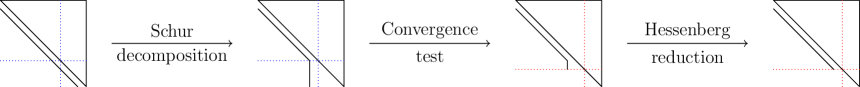
Figure 1: A visual illustration of AED.

Because algorithms for Hessenberg reduction and Schur decomposition already exist for quaternion matrices, we have gathered all the necessary building blocks for performing AED for quaternion matrices with the help of the eigenvalue swapping algorithm.

We note that in a multishift variant of the quaternion QR algorithm, the undeflatable eigenvalues left by AED can be used as the shifts. However, the development of the small-bulge multishift QR algorithm is beyond the scope of this work.

Although the AED technique was developed to enhance the convergence of the small-bulge multishift QR algorithm [4], according to [22], even the very traditional Francis QR algorithm can be accelerated by AED. It is natural to ask if the AED technique remains effective when applied to quaternion matrices. Fortunately, existing theoretical analyses on AED [5, 24] suffice to predict the effectiveness of AED in the quaternion QR algorithm. In fact, by embedding the quaternion matrix into a complex matrix with double the dimensions, the AED technique—essentially the extraction of Ritz pairs—has more opportunities to detect converged eigenvalues compared to classical deflation based on testing subdiagonal entries.

Finally, we remark that the eigenvalue swapping algorithm also allows us to develop other advanced algorithms. For example, the Krylov–Schur algorithm for solving large-scale eigenvalue problems [31], which is closely related to AED [22, 24], also carries over to quaternion matrices.

5 Numerical experiments

In this section, we conduct some numerical experiments to evaluate the effectiveness of the proposed algorithms. These experiments were carried out using MATLAB 2023a and the QTFM toolbox version 3.4 [27], on a Linux cluster comprising ten 48-core Intel Xeon Gold 6342 CPUs, each with a frequency of 2.80 GHz, and 20 GB of memory. We ran our MATLAB programs on one CPU in this cluster. All computations were performed using IEEE double-precision floating-point numbers, with a machine precision of $\epsilon=2^{-52}\approx 2.22\times 10^{-16}$.

We define two classes of randomly generated quaternion matrices as follows.

• fullrand: A dense square matrix whose entries are randomly generated.

• hessrand: A dense upper Hessenberg matrix whose nonzero entries are randomly generated.

These class of matrices are frequently used to test non-Hermitian dense eigensolvers [14, 15, 19]. For each nonzero entry, we generate a random unit quaternion $\omega$ using the randq() function from the QTFM toolbox, and then multiply it by a random real number $\alpha$ uniformly distributed in the range of $[0,1]$. The resulting value of $\omega\cdot\alpha$ is then used as the matrix entry.

5.1 Performance tests

In the following we test the effectiveness of the AED technique in the quaternion QR algorithm (i.e., Algorithm 1). The size of the AED window, $n_{\mathsf{win}}$, is adaptively adjusted based on the matrix size $n$, following the strategy used in LAPACK’s IPARMQ [8]. The threshold for skipping a QR sweep, commonly known as ‘NIBBLE’, is set to $14\%$, the default value used in LAPACK’s IPARMQ [8].

Tables 1 and 2 present the detailed results for fullrand and hessrand matrices, respectively, with matrix dimensions ranging from $64\times 64$ to $1024\times 1024$. The tables contain the total number of QR sweeps, total execution time (in seconds), time spent constructing the Schur vectors $\bm{Q}$, and time spent on AED for each test case.

The results show that the quaternion QR algorithm incorporated with AED consistently performs fewer QR sweeps and has a shorter execution time than the original quaternion QR algorithm. The reduction in QR sweeps becomes more significant as the matrix size increases (see Figure 2), leading to a substantial decrease in total execution time.

Although our implementations are only preliminary ones in MATLAB, we expect that the AED technique remains highly effective in a high performance implementation of the quaternion QR algorithm, since the number of QR sweeps can be significantly reduced.

Table 1: Performance tests on the QR algorithm, with and without AED, for fullrand matrices.

strategy	matrix size	total QR sweeps	total time	time to construct Q	time for AED
QR+AED	64	173	$6.88\times 10^{0}$	$7.08\times 10^{-1}$	$3.34\times 10^{0}$
QR	64	200	$4.11\times 10^{0}$	$8.12\times 10^{-1}$	N/A
QR+AED	128	267	$2.39\times 10^{1}$	$2.73\times 10^{0}$	$1.13\times 10^{1}$
QR	128	399	$1.95\times 10^{1}$	$4.26\times 10^{0}$	N/A
QR+AED	256	420	$9.66\times 10^{1}$	$1.26\times 10^{1}$	$4.05\times 10^{1}$
QR	256	784	$1.25\times 10^{2}$	$2.81\times 10^{1}$	N/A
QR+AED	512	647	$6.86\times 10^{2}$	$1.20\times 10^{2}$	$2.21\times 10^{2}$
QR	512	1530	$1.61\times 10^{3}$	$3.82\times 10^{2}$	N/A
QR+AED	1024	935	$8.63\times 10^{3}$	$1.75\times 10^{3}$	$1.60\times 10^{3}$
QR	1024	3095	$2.13\times 10^{4}$	$5.23\times 10^{3}$	N/A

Table 2: Performance tests on the QR algorithm, with and without AED, for hessrand matrices.

strategy	matrix size	total QR sweeps	total time	time to construct Q	time for AED
QR+AED	64	159	$7.84\times 10^{0}$	$7.41\times 10^{-1}$	$4.14\times 10^{0}$
QR	64	202	$4.13\times 10^{0}$	$8.15\times 10^{-1}$	N/A
QR+AED	128	262	$2.86\times 10^{1}$	$3.02\times 10^{0}$	$1.49\times 10^{1}$
QR	128	406	$2.06\times 10^{1}$	$4.43\times 10^{0}$	N/A
QR+AED	256	330	$8.49\times 10^{1}$	$8.82\times 10^{0}$	$4.57\times 10^{1}$
QR	256	880	$1.41\times 10^{2}$	$3.11\times 10^{1}$	N/A
QR+AED	512	427	$6.12\times 10^{2}$	$9.33\times 10^{1}$	$2.59\times 10^{2}$
QR	512	1925	$2.20\times 10^{3}$	$5.13\times 10^{2}$	N/A
QR+AED	1024	919	$9.52\times 10^{3}$	$1.87\times 10^{3}$	$2.02\times 10^{3}$
QR	1024	3915	$2.57\times 10^{4}$	$6.32\times 10^{3}$	N/A

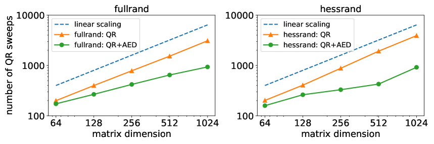
Figure 2: The number of QR sweeps with respect to the matrix dimension.

5.2 Stability tests

In the following, we evaluate the backward stability of the QR algorithm, as well as the eigenvector computation. For the Schur decomposition $\bm{A}=\bm{Q}\bm{T}\bm{Q}^{\mathsf{H}}$ and the spectral decomposition $\bm{A}=\bm{X}\bm{\Lambda}\bm{X}^{-1}$, we measure the following quantities:

$$e_{1}=\frac{1}{\sqrt{n}}\lVert\bm{Q}^{\mathsf{H}}\bm{Q}-\bm{I}\rVert_{\mathsf{F}},\qquad e_{2}=\frac{\lVert\bm{Q}^{\mathsf{H}}\bm{A}\bm{Q}-\bm{T}\rVert_{\mathsf{F}}}{\lVert\bm{A}\rVert_{\mathsf{F}}},\qquad e_{3}=\frac{\lVert\bm{A}\bm{X}-\bm{X}\bm{\Lambda}\rVert_{\mathsf{F}}}{(\lVert\bm{A}\rVert_{\mathsf{F}}+\lVert\bm{\Lambda}\rVert_{\mathsf{F}})\lVert\bm{X}\rVert_{\mathsf{F}}}.$$

The results for fullrand and hessrand matrices are listed in Tables 3 and 4, respectively. We can see that both the AED strategy and the eigenvector computation are numerically stable. In most test cases, when the AED strategy is incorporated, the backward errors are slightly lower. This is likely because AED effectively reduces the total number of floating-point operations.

Table 3: Stability tests on the QR algorithm, with and without AED, for fullrand matrices.

strategy	matrix size	$e_{1}$	$e_{2}$	$e_{3}$
QR+AED	64	$9.2\times 10^{-15}$	$6.4\times 10^{-15}$	$6.4\times 10^{-16}$
QR	64	$9.0\times 10^{-15}$	$6.4\times 10^{-15}$	$7.2\times 10^{-16}$
QR+AED	128	$1.3\times 10^{-14}$	$8.5\times 10^{-15}$	$6.9\times 10^{-16}$
QR	128	$1.3\times 10^{-14}$	$9.2\times 10^{-15}$	$7.0\times 10^{-16}$
QR+AED	256	$1.7\times 10^{-14}$	$1.1\times 10^{-14}$	$6.0\times 10^{-16}$
QR	256	$1.7\times 10^{-14}$	$1.2\times 10^{-14}$	$6.6\times 10^{-16}$
QR+AED	512	$2.1\times 10^{-14}$	$1.3\times 10^{-14}$	$5.1\times 10^{-16}$
QR	512	$2.5\times 10^{-14}$	$1.7\times 10^{-14}$	$6.9\times 10^{-16}$
QR+AED	1024	$2.5\times 10^{-14}$	$1.6\times 10^{-14}$	$4.3\times 10^{-16}$
QR	1024	$3.4\times 10^{-14}$	$2.5\times 10^{-14}$	$6.8\times 10^{-16}$

Table 4: Stability tests on the QR algorithm, with and without AED, for hessrand matrices.

strategy	matrix size	$e_{1}$	$e_{2}$	$e_{3}$
QR+AED	64	$1.0\times 10^{-14}$	$6.1\times 10^{-15}$	$3.9\times 10^{-16}$
QR	64	$8.8\times 10^{-15}$	$6.0\times 10^{-15}$	$4.4\times 10^{-16}$
QR+AED	128	$1.3\times 10^{-14}$	$8.0\times 10^{-15}$	$2.9\times 10^{-16}$
QR	128	$1.3\times 10^{-14}$	$8.7\times 10^{-15}$	$2.8\times 10^{-16}$
QR+AED	256	$1.7\times 10^{-14}$	$1.0\times 10^{-14}$	$1.7\times 10^{-16}$
QR	256	$1.8\times 10^{-14}$	$1.3\times 10^{-14}$	$2.1\times 10^{-16}$
QR+AED	512	$2.2\times 10^{-14}$	$1.2\times 10^{-14}$	$1.2\times 10^{-16}$
QR	512	$2.7\times 10^{-14}$	$1.8\times 10^{-14}$	$8.8\times 10^{-17}$
QR+AED	1024	$2.3\times 10^{-14}$	$9.2\times 10^{-15}$	$4.8\times 10^{-17}$
QR	1024	$3.6\times 10^{-14}$	$2.3\times 10^{-14}$	$5.8\times 10^{-17}$

6 Conclusions

In this paper, we discuss several aspects of the dense non-Hermitian quaternion eigenvalue problem. We develop algorithms for eigenvector computation from the Schur form, and the eigenvalue swapping algorithm. As an application of the eigenvalue swapping algorithm, we discuss the aggressive early deflation (AED) technique for the quaternion QR algorithm. These developments fill the gap in existing dense quaternion eigensolvers—we have come to a point where no theoretical obstacle remains for the non-Hermitian quaternion QR algorithm. What is left in this direction is mainly the work of high performance computing—how to implement efficient dense quaternion eigensolvers. This includes, but not limited to, the development of efficient quaternion BLAS libraries [12, 32], efficient Hessenberg reduction [20, 21, 28], small-bulge multishift QR algorithm [4, 8, 14, 15], level-3 eigenvalue reordering algorithm [13, 23], and level-3 eigenvector computation [29].

References

- [1] Stephen L. Adler. Quaternionic Quantum Mechanics and Quantum Fields. Oxford Univ. Press, New York, NY, USA, 1995.
- [2] E. Anderson, Z. Bai, C. Bischof, L. S. Blackford, J. Demmel, J. Dongarra, J. Du Croz, A. Greenbaum, S. Hammarling, A. McKenney, and D. Sorensen. LAPACK Users’ Guide. SIAM, Philadelphia, PA, USA, 3rd edition, 1999. doi:10.1137/1.9780898719604.
- [3] Zhaojun Bai and James W. Demmel. On a block implementation of Hessenberg multishift QR iteration. Int. J. High Speed Comput., 1(1):97–112, 1989. doi:10.1142/S0129053389000068.
- [4] Karen Braman, Ralph Byers, and Roy Mathias. The multishift QR algorithm. Part I: Maintaining well-focused shifts and level 3 performance. SIAM J. Matrix Anal. Appl., 23(4):929–947, 2002. doi:10.1137/S0895479801384573.
- [5] Karen Braman, Ralph Byers, and Roy Mathias. The multishift QR algorithm. Part II: Aggressive early deflation. SIAM J. Matrix Anal. Appl., 23(4):948–973, 2002. doi:10.1137/S0895479801384585.
- [6] J. L. Brenner. Matrices of quaternions. Pacific J. Math., 1(3):329–335, 1951.
- [7] Angelika Bunse-Gerstner, Ralph Byers, and Volker Mehrmann. A quaternion QR algorithm. Numer. Math., 55(1):83–95, 1989. doi:10.1007/bf01395873.
- [8] Ralph Byers. LAPACK 3.1 xHSEQR: Tuning and implementation notes on the small bulge multi-shift QR algorithm with aggressive early deflation. Technical report, 2007. LAPACK Working Notes No. 187.
- [9] J. G. F. Francis. The QR transformation: a unitary analogue to the LR transformation. I. Comput. J., 4(3):265–271, 1961. doi:10.1093/comjnl/4.3.265.
- [10] J. G. F. Francis. The QR transformation. II. Comput. J., 4(4):332–345, 1962. doi:10.1093/comjnl/4.4.332.
- [11] Georgi Georgiev, Ivan Ivanov, Milena Mihaylova, and Tsvetelina Dinkova. An algorithm for solving a Sylvester quaternion equation. Proc. Annual Conf. Rousse Univ. and Sc. Union, 48:35–39, 2009.
- [12] Kazushige Goto and Robert van de Geijn. High-performance implementation of the level-3 BLAS. ACM Trans. Math. Software, 35(1):4, 2008. doi:10.1145/1377603.1377607.
- [13] Robert Granat, Bo Kågström, and Daniel Kressner. Parallel eigenvalue reordering in real Schur forms. Concurrency and Computat.: Pract. Exper., 21(9):1225–1250, 2009. doi:10.1145/2699471.
- [14] Robert Granat, Bo Kågström, and Daniel Kressner. A novel parallel QR algorithm for hybrid distributed memory HPC systems. SIAM J. Sci. Comput., 32(4):2345–2378, 2010. doi:10.1137/090756934.
- [15] Robert Granat, Bo Kågström, Daniel Kressner, and Meiyue Shao. Algorithm 953: Parallel library software for the multishift QR algorithm with aggressive early deflation. ACM Trans. Math. Software, 41(4):29, 2015. doi:10.1145/2699471.
- [16] Zhigang Jia, Musheng Wei, Mei-Xiang Zhao, and Yong Chen. A new real structure-preserving quaternion QR algorithm. J. Comput. Appl. Math., 343:26–48, 2018. doi:10.1016/j.cam.2018.04.019.
- [17] R. E. Johnson. On the equation over an algebraic division ring. Bull. Amer. Math. Soc, 50(4):202–207, 1944.
- [18] Katherine Jones-Smith. Non-Hermitian Quantum Mechanics. PhD thesis, Case Western Reserve University, 2010.
- [19] Bo Kågström, Daniel Kressner, and Meiyue Shao. On aggressive early deflation in parallel variants of the QR algorithm. In Kristján Jónasson, editor, Applied Parallel and Scientific Computing (PARA 2010), pages 1–10, Berlin, Heidelberg, Germany, 2012. Springer-Verlag. doi:10.1007/978-3-642-28151-8_1.
- [20] Lars Karlsson and Bo Kågström. Parallel two-stage reduction to Hessenberg form using dynamic scheduling on shared-memory architectures. Parallel Comput., 37:771–782, 2011. doi:10.1016/j.parco.2011.05.001.
- [21] Lars Karlsson and Bo Kågström. Efficient reduction from block Hessenberg form to Hessenberg form using shared memory. In Kristján Jónasson, editor, Applied Parallel and Scientific Computing (PARA 2010), pages 258–268, Berlin, Heidelberg, Germany, 2012. Springer-Verlag. doi:10.1007/978-3-642-28145-7_26.
- [22] Daniel Kressner. Numerical Methods for General and Structured Eigenvalue Problems. Springer-Verlag, Berlin, Heidelberg, Germany, 2005. doi:10.1007/3-540-28502-4.
- [23] Daniel Kressner. Block algorithms for reordering standard and generalized Schur forms. ACM Trans. Math. Software, 32(4):521–532, 2006. doi:10.1145/1186785.1186787.
- [24] Daniel Kressner. The effect of aggressive early deflation on the convergence of the QR algorithm. SIAM J. Matrix Anal. Appl., 30(2):805–821, 2008. doi:10.1137/06067609X.
- [25] Nicolas Le Bihan and Jérôme Mars. Singular value decomposition of quaternion matrices: a new tool for vector-sensor signal processing. Signal Process., 84(7):1177–1199, 2004. doi:10.1016/j.sigpro.2004.04.001.
- [26] Nicolas Le Bihan and Stephen J. Sangwine. Quaternion principal component analysis of color images. In Proceedings of the 2003 International Conference on Image Processing, pages 809–812. IEEE, 2003. doi:10.1109/icip.2003.1247085.
- [27] Nicolas Le Bihan and Stephen J. Sangwine. Quaternion and octonion toolbox for MATLAB, 2013. URL: https://qtfm.sourceforge.io/.
- [28] Gregorio Quintana-Ortí and Robert van de Geijn. Improving the performance of reduction to Hessenberg form. ACM Trans. Math. Software, 32(2):180–194, 2006. doi:10.1145/1141885.1141887.
- [29] Angelika Schwarz, Carl Christian Kjelgaard Mikkelsen, and Lars Karlsson. Robust parallel eigenvector computation for the non-symmetric eigenvalue problem. Parallel Comput., 100:102707, 2020. doi:10.1016/j.parco.2020.102707.
- [30] Yanjun Shao. Aggressive early deflation in the quaternion QR algorithm. Bachelor’s thesis, School of Data Science, Fudan University, 2023. (In Chinese).
- [31] G. W. Stewart. A Krylov–Schur algorithm for large eigenproblems. SIAM J. Matrix Anal. Appl., 23(3):601–614, 2002. doi:10.1137/S0895479800371529.
- [32] David B. Williams-Young and Xiaosong Li. On the efficacy and high-performance implementation of quaternion matrix multiplication, 2019. arXiv preprint 1903.05575. doi:10.48550/arXiv.1903.05575.
- [33] Fuzhen Zhang. Quaternions and matrices of quaternions. Linear Algebra Appl., 251:21–57, 1997. doi:10.1016/0024-3795(95)00543-9.