1 Introduction

Hypothesis testing involves making a discrete choice and constitutes the most basic form of decision-making under uncertainty. It occupies a central role in practice, serving as an assessment of evidence in most scientific research. Testing, however, rarely occurs in isolation. In a broader system-level context, outcomes of a test have downstream implications, such as deploying a new drug, adding a new feature to a commercial product, or publishing a scientific finding. While all parties involved are affected, stakeholders may be differentially impacted by the results. In the other direction, upstream of the phase of data collection, these same parties may have additional, potentially private information about the object of study and make choices that affect the data generation. For example, a pharmaceutical company sponsoring a phase III clinical trial for a candidate drug implicitly has a belief about the drug’s efficacy and chooses to run a trial accordingly. In this way, the distribution of the data observed, and thus the performance of any method for statistical decision-making, is altered by strategic behavior of the agents involved.

In this paper, we study hypothesis testing based on data collected from a heterogeneous population of agents, and analyze how their strategic behavior impacts the design of optimal statistical tests. More specifically, we consider a principal that seeks to carry out a collection of hypothesis tests. Each test is controlled by an agent that possesses private information—not known to the principal—and this private information can differ across agents. Our main contribution is to show how to design a protocol for hypothesis testing that yields statistically optimal results even when the private information of the agents is not known in advance.

As a simple illustration, suppose there are two agent types: a “good” type with a high prior probability of being non-null and a “bad” type with a low prior probability of being non-null. The decision-maker evaluates agents using $p$-value thresholds, which determine the stringency of the test: smaller thresholds reduce false positives but also reduce true discoveries. For a heterogeneous collection of tests, one natural measure of aggregate performance is based on the false discovery rate and true discovery rate; cf. equations (5a) and (5b). The false discovery rate (FDR) corresponds to the fraction of rejections that are false, while the true discovery rate (TDR) corresponds to the rate of true discoveries across the mixture of types, and captures a notion of overall power.

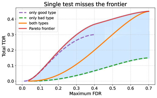
Figure 1: trade-offs between FDR and TDR for a population with two agent types: “good” and “bad”. The light-blue region corresponds to all FDR-TDR pairs that can be achieved by any testing protocol. Its upper boundary (solid red) defines the Pareto frontier that can be achieved by an oracle that knows the agent type associated with each observation, and applies different test thresholds to each. The orange solid curve shows the result of applying a single uniform test to the full agent population. The dotted lines show the performance of applying a single test to only the “good” agents (purple line), and only the “bad” agents (green line); applying these two protocols also requires knowledge of the agent type.

Figure 1 illustrates how heterogeneity undermines efficiency. The light-blue region shows all achievable (FDR, TDR) pairs when the decision-maker is permitted to apply different tests to each agent type; the upper boundary of this region (marked in a solid red line) corresponds to the oracle Pareto frontier that could be achieved if the principal were given access to the hidden agent type. A single threshold applied uniformly across both types (orange curve) lies substantially below the Pareto frontier. We can also compare to two other single threshold protocols that do require knowledge of agent type. Applying a test to only the “good” agents yields the purple curve; it has a more favorable trade-off, but still lies below the Pareto frontier. Testing only the “bad” type (green curve) defines the lower boundary of the achievable region.

When the agent types are known, it is possible to tailor thresholds to different agent types so as to balance error trade-offs more effectively: moderate thresholds for good type to increase power, and stricter thresholds for bad types to limit false discoveries. It is exactly this tailored choice of thresholds that yields the oracle Pareto frontier (red curve). However, in practice, agent types are not directly observable, so we are led to the following question:

The main contribution of this paper is to answer this question in a constructive way: we both characterize when it is possible to match the oracle and provide a concrete procedure for constructing testing protocols that do so. The key insight in our work is that, because agents are assumed to behave strategically, their actions can reveal private information. We leverage this by offering a menu of possible statistical tests, each paired with an associated payoff structure—together forming what we call a contract. We show that it is possible to design a menu of contracts such that an agent’s choice of contract reveals their private information, and moreover, such that each agent selects the statistical threshold that is optimal for their type. This design yields a testing protocol whose statistical error trade-offs match the oracle Pareto frontier, even though the principal has no a priori knowledge of agent types.

1.1 Our contributions

We study a game-theoretic model of hypothesis testing with a heterogeneous population of strategic agents. The decision-maker (principal) designs a hypothesis testing protocol, while agents decide whether to participate based on private information and expected payoffs. Participation requires a fixed cost, and agents receive a reward if they pass the test. We formalize this interaction through a menu of statistical contracts, as defined precisely in equation (1), where each contract specifies the testing protocol, the upfront cost, and the reward.

There is an evolving line of work on principal-agent testing [Tet16, Bat+22, Bat+23, SBW24, HCC25, VWN24], and within this context, our analysis makes the following contributions:

• Menus for heterogeneous agents. Prior studies largely focus on single agents or uniform tests that control only false discoveries. We instead analyze heterogeneous populations and the optimal trade-off between the two competing types of statistical error. We show that the principal can implement a menu of statistical contracts to fully elicit agents’ private information and assign type-optimal thresholds, thereby matching the statistical performance of an oracle given access to agent types in advance. Our main result (Theorem 1) fully characterizes all separating menus that have this instance-adaptive optimality.

• Costs of elicitation. A natural concern is whether eliciting private information requires substantial financial resources. We show that the principal can construct menus (see Corollary 2, illustrated in Figure 2) that achieve statistical efficiency while incurring arbitrarily small financial cost relative to offering a single contract. This establishes that optimal error trade-offs can be attained essentially “for free.”

• Connection to scoring rules and test structure. An interesting by-product of our analysis is to establish a connection between menu design and strictly proper scoring rules (Section 3.1.3). However, in contrast to classical scoring rules, the principal cannot directly specify the agent’s utility but must induce it indirectly through contracts tied to hypothesis tests. When all contract parameters are flexible, full elicitation is possible. Under constraints—e.g., when rewards are fixed—the structure of the statistical testing problem itself dictates which types can be elicited and at what cost (see Corollary 3).

Taken together, our results illustrate a key principle: heterogeneity and strategic behavior, which are often viewed as obstacles, can instead be leveraged as tools. By carefully designing testing protocols and incentives, the principal can transform private information and self-interested participation into a mechanism for statistically optimal decision-making—and remarkably, this can be achieved with minimal financial cost.

1.2 Related work

Our work connects to several strands of literature at the intersection of contract theory, statistical decision-making, and strategic behavior. In addition, by comparing statistical performance to an oracle, our work shares the spirit of statistical literature on adaptive estimation and testing.

Let us begin by discussing the connections to screening and incentive design in contract theory [LM01, BD04, Sal05]. Here the focus of the study is how a principal can elicit private information from heterogeneous agents by offering a menu of contracts. Classical applications include nonlinear pricing [MR78, MR84], auctions [Mye81, MR84a], and regulation [BM82, LT93]. Our work shares this idea of elicitation, but shows that hypothesis tests themselves, paired with suitable payoff structures, can act as screening devices. Related recent work has used experimental designs as screening mechanisms [WY25, Yod22, Wan23, JV25], underscoring the broader potential of statistical objects for information elicitation. Elicitation is naturally connected to the notion of proper scoring rules [Bri50, Goo52, McC56, Sav71, GR07], which correspond to utility functions designed to elicit truthful reports. Our mechanism also encourages truthful elicitation, but with the important distinction that we have only indirect and partial control over the utility via the specification of the hypothesis test.

More broadly, our work relates to a growing literature on strategic behavior in decision-making, where agents may manipulate data, analysis, or participation to influence outcomes. A prominent example is $p$-hacking, where researchers adjust analyses to obtain significant results, inflating false positives. The statistics literature has responded with selective inference methods [TT15, Ber+13], while economic analyses take a game-theoretic perspective. For instance, [MM24] designed critical values robust to strategic manipulation, and [JV25] studied how differences in private costs and incentives shape optimal publication rules. [Spi18] showed that restricting researchers to fixed-bias estimators can improve inference when planner’s and researcher’s objectives diverge. Beyond $p$-hacking, the machine learning community has explored mechanism design under strategic manipulation of data, such as altering features or labels to influence classifiers [Har+16, Don+18] or regressions [DFP10, PPP04, Che+18]. In contrast, the strategic behavior in our setting takes the form of participation decisions: agents cannot alter test outcomes directly, but they can choose whether to engage. This captures environments where experiments are preregistered or data collection is externally verified, so participation is the primary lever for influence.

As noted above, our work contributes directly to the evolving literature on principal–agent hypothesis testing. [Tet16] provided an early analysis linking type I error control to a cost–profit ratio. Subsequent work [Bat+22, Bat+23, SBW24, HCC25] expanded the framework to incorporate risk aversion, stochastic rewards, and simultaneous control of type I and II errors. Our contribution departs from this line by focusing on heterogeneous populations and showing how menus of contracts can achieve type-optimal thresholds and optimal error trade-offs. In doing so, we integrate heterogeneity, screening, and strategic participation into a unified framework that ties statistical objectives to incentive-compatible design.

Finally, we define optimality in this paper with reference to an oracle that is given direct access to the agents’ private information. Our work thus shares the spirit of work on adaptive estimation and testing (e.g., [CL06, Lep90, Spo96]). This classical work considers tests or estimators that adapt to unknown problem structure such as smoothness or sparsity, whereas we study adaptation to the unknown private information of a collection of agents.

Paper organization:

Section 2 formalizes the menu-based principal–agent testing framework, specifying agents’ strategic behavior and the principal’s statistical objectives. Section 3 is devoted to the statement of main results on separating menus (Section 3.1), along with results on menu constructions that satisfy pre-specified criteria (Section 3.2). Our central theorem (Theorem 1), stated in Section 3.1.1, characterizes all separating menus that elicit private information and implement type-optimal thresholds for arbitrary heterogeneous populations. In Section 3.1.2, we show how this theorem allows the principal to match the statistical performance of the oracle (Corollary 1). We highlight a connection to proper scoring rules in Section 3.1.3, and analyze the financial costs of elicitation in Section 3.1.4. In Section 3.2, we study menu constructions under two practical design criteria: one that minimizes the principal’s financial cost, showing that information elicitation can be achieved “for free,” and another that addresses settings where the principal can only partially specify contracts. We illustrate the implications of these results through synthetic examples. We conclude in Section 4 with a discussion. We examine the robustness of menu-based testing to model misspecification in Appendix C.

2 Mathematical Model

In this section, we formalize the problem by specifying the structure of the hypothesis tests, the principal–agent interaction, the agent’s utility maximization problem, and the principal’s statistical decision problem.

2.1 Strategic hypothesis test

We consider a game-theoretic framework involving two parties: a principal, who serves as a statistical regulator, and an agent. The principal’s role is to approve or deny proposals submitted by agents. To make these decisions, the principal offers the agent a menu of statistical contracts at different costs (described below). Agents observe the entire menu and choose whether to select one contract from the menu or to opt out, based on their private information and utility. Upon selecting a contract, data is collected and reported to the principal, who conducts a hypothesis test according to the terms specified in the chosen contract. We make all of these steps precise below.

Hypothesis space and agent type

We assume that there exists a hidden random parameter $\theta$, which takes two possible values $\theta\in\Theta=\{\theta_{0},\theta_{1}\}$ and represents the latent quality of any proposal. The null value $\theta_{0}$ corresponds to an ineffective proposal and the non-null value $\theta_{1}$ corresponds to an effective proposal. Neither the principal nor the agent knows the true value of $\theta$. However, the agent has private knowledge of a prior distribution $\mathbb{Q}$ over $\Theta$, which is inaccessible to the principal. While the principal could attempt to ask the agent directly about $\mathbb{Q}$, there is no guarantee the agent would report it truthfully. As we later show, the principal can instead offer a menu of contracts designed to elicit information about $\mathbb{Q}$.

We consider a setting with a population of agents, each characterized by a potentially distinct prior distribution $\mathbb{Q}$. Since the parameter space is binary, this distribution is fully specified by the prior null probability $q:\,\!=\mathbb{Q}(\theta=\theta_{0})$. We can classify agents according to the value of their prior null: in particular, we say that an agent is of type $q$ if he has prior null probability equal to $q$. The overall population of agents consists of different types occurring with a certain frequency, and we let $\mathbb{T}$ denote a distribution over possible types $q$. We do not assume that the principal knows $\mathbb{T}$.

The principal-agent interaction

We now formalize the notion of a statistical contract and its role in the principal-agent interaction. The principal aims to approve effective proposals and deny ineffective ones by conducting hypothesis tests. To this end, she designs a contract menu, meaning a collection of contracts indexed by reported type $p\in[0,1]$, where each contract specifies how the hypothesis test will be conducted. Any contract menu takes the form

$$\mathscr{M} :\,\!=\Big\{(\tau_{p},R_{p},C_{p})\mid p\in\mathcal{P}\Big\},$$ (1)

where $\mathcal{P}\subseteq[0,1]$ is a subset of values associated with contracts, and any contract is defined by a triplet with the following components:

• a threshold $\tau_{p}\in[0,1]$ used in the principal’s binary hypothesis test, as described below.

• the reward $R_{p}$ received by the agent if the proposal is approved, and

• the cost $C_{p}$ paid by the agent to opt in (and hence to generate evidence).

The agent observes the full contract menu (1) before making any selection. Based on his private information $q$, the agent decides whether to opt in or opt out. If the agent opts in, he selects a type $p\in\mathcal{P}$ to the principal. The contract corresponding to this reported type $p$ is then executed.

We now describe how each possible contract is executed. Let $\{\mathbb{P}_{\theta}\mid\theta\in\Theta\}$ be a family of probability distributions indexed by $\theta$. These are the possible distributions generating the data $X$ that the principal uses for decision-making. The family of distributions is known to both the principal and agent. Without loss of generality, we assume the variable $X$ is a $p$-value, meaning that distribution under the null hypothesis is uniform:

$$\mathbb{P}_{\theta_{0}}(X\leq\tau)=\tau\qquad\mbox{for any choice of threshold $\tau\in[0,1]$.}$$

When an agent with parameter $\theta$ chooses a statistical contract $(\tau_{p},R_{p},C_{p})$, he spends $C_{p}$ dollars to conduct an experiment, which yields a random variable $X$ drawn from distribution $\mathbb{P}_{\theta}$. The principal then approves the proposal if $X\leq\tau_{p}$ and denies it otherwise.

If the principal approves, the agent receives $R_{p}$ dollars in return, resulting in a net payoff of $R_{p}-C_{p}$ dollars after accounting for the up-front cost. Otherwise, when the principal denies the proposal, the agent receives no reward, thus losing a net of $C_{p}$ dollars. The principal-agent interaction is summarized as follows:

2.2 Utility-maximizing agents

We assume that agents are strategic decision-makers who act to maximize expected utility. Each agent is risk-neutral, meaning that their utility is equivalent to their expected gain in wealth. The agent’s utility, determined jointly by their own actions and the principal’s decision, can fall into one of three possible outcomes:

• If the agent chooses contract $(\tau_{p},R_{p},C_{p})$ and the principal approves the proposal, the agent gains $R_{p}-C_{p}$ in wealth.

• If the agent chooses contract $(\tau_{p},R_{p},C_{p})$ and the principal denies the proposal, the agent loses $C_{p}$ in wealth.

• If the agent chooses to opt out, he neither gains nor loses in wealth.

For an agent who opts into the contract indexed by $p$, his change in wealth is given by the random variable $R_{p}\>\mathbb{I}(X\leq\tau_{p})-C_{p}$. Since the prior distribution $\mathbb{Q}$ of any agent is specified by the null probability $q=\mathbb{Q}(\theta=\theta_{0})$, we define the agent’s expected utility as

$$\operatorname{Util}(q;p):\,\!=\mathbb{E}_{\begin{subarray}{c}\theta\sim\mathbb{Q}\\ X\sim\mathbb{P}_{\theta}\end{subarray}}\Big[R_{p}\>\mathbb{I}(X\leq\tau_{p})-C_{p}\Big].$$

Given a contract menu $\mathscr{M}$ with support $\mathcal{P}$, we assume that agents are wealth-maximizing, meaning that the behavior of an agent of type $q$ is characterized by the selection function

$$\varphi_{\mathscr{M}}(q) :\,\!=\arg\max_{p\in\mathcal{P}}\operatorname{Util}(q;p).$$ (2a)

If $$\operatorname{Util}(q;\varphi_{\mathscr{M}}(q))\geq 0$$, the agent accepts the chosen contract; otherwise, the agent opts out.

To make the utility expression more explicit, recall the type I error and power functions of a simple-simple hypothesis test with threshold $\tau\in[0,1]$:

$$\beta_{0}(\tau):\,\!=\mathbb{P}_{\theta_{0}}(X\leq\tau)=\tau\quad\mbox{and}\quad\beta_{1}(\tau):\,\!=\mathbb{P}_{\theta_{1}}(X\leq\tau).$$ (2b)

With this notation, the expected utility of an agent of type $q$ selecting contract $p$ can be written as

$$\operatorname{Util}(q;p) =qR_{p}\big[\beta_{0}(\tau_{p})-\beta_{1}(\tau_{p})\big]+\big[R_{p}\beta_{1}(\tau_{p})-C_{p}\big].$$ (2c)

See Section D.1 for the proof of this claim.

Notice the utility (2c) is linear in the agent’s prior null probability $q$ with slope $R_{p}[\beta_{0}(\tau_{p})-\beta_{1}(\tau_{p})]$. We are interested in the case with non-trivial power, i.e., $\beta_{1}(\tau_{p})>\beta_{0}(\tau_{p})$, in which case the slope is negative. Thus, agents with smaller $q$ (more optimistic priors) derive greater expected utility from any given contract. Moreover, the utility is nondecreasing in $\tau_{p}$, since both the type I error $\beta_{0}(\tau_{p})$ and the power $\beta_{1}(\tau_{p})$ are nondecreasing.

2.3 Statistical decision problem of the principal

At a high level, the principal’s objective is to design a menu that controls the two types of error in a binary hypothesis test. The menu should achieve a desired balance between type I errors (where $\theta=\theta_{0}$ but the principal approves) and type II errors (where $\theta=\theta_{1}$ but the principal denies). We consider two specifications of this trade-off below: (a) she may wish to minimize a weighted sum of the errors, or (b) to maximize total discovery rate subject to a constraint on the false discovery rate. In either case, the key feature is that the principal’s optimal decision rule depends on the agent’s prior null probability $q$. When the null is more likely (large $q$), a lenient test with a large threshold risks too many false positives, so the optimal test should be more stringent. Conversely, when the null is unlikely (small $q$), the principal can afford to be more permissive to avoid unnecessary false negatives.

We use $\tau_{q}$ to denote the principal’s ideal threshold for an agent with prior $q$, and refer to it as the type-optimal threshold. We describe two concrete cases next.

Weighted sum of type I and type II error.

In many settings, the principal’s cost of making a type I error is not the same as that of type II error. Suppose type I errors incur cost $\omega_{1}$ and type II errors incur cost $\omega_{2}$. For an agent of type $q$, if the principal deployed a test at level $\tau$, the associated Bayes risk (BR) is given by

$$\operatorname{BR}_{\omega}(q,\tau)=\omega_{1}\cdot q\cdot\underbrace{\mathbb{P}_{\theta_{0}}(X\leq\tau)}_{\equiv\tau}+\omega_{2}\cdot(1-q)\cdot\underbrace{\mathbb{P}_{\theta_{1}}(X>\tau)}_{\equiv 1-\beta_{1}(\tau)}.$$ (3)

Classical results show that the optimal decision rule for the Bayes risk $\operatorname{BR}_{\omega}$ is to threshold the likelihood ratio statistic at level $q\omega_{1}/(1-q)\omega_{2}$. Thus, the optimal $p$-values $X$ for the principal are those obtained from the likelihood ratio statistic. Concretely, if we let $X\mapsto\mathcal{L}(X)$ be the function mapping $X$ to the likelihood ratio, then the type-optimal threshold on the $p$-value scale is

$$\tau_{q}\equiv\tau_{q}(\omega):\,\!=\mathcal{L}^{-1}\bigg(\frac{q\omega_{1}}{(1-q)\omega_{2}}\bigg).$$ (4)

Maximizing TDR subject to FDR control.

Alternatively, the principal might wish to maximize the expected true discovery rate (TDR) while controlling the false discovery rate (FDR) at a target level $\alpha$. For an agent of type $q$, the FDR associated with the hypothesis test with threshold $\tau$ is given by

$$\operatorname{FDR}(q,\tau) :\,\!=\mathbf{P}\Big[\theta\in\Theta_{0}\mid X\leq\tau\Big]=\frac{q\beta_{0}(\tau)}{q\beta_{0}(\tau)+(1-q)\beta_{1}(\tau)},$$ (5a)

which corresponds to the probability that a proposal approved is actually ineffective. On the other hand, the TDR for a given $$(q,\tau)$$-pair is given by

$$\operatorname{TDR}(q,\tau):\,\!=(1-q)\beta_{1}(\tau),$$ (5b)

which represents the probability of correctly approving non-null proposals from agent $q$ when using threshold $\tau$. Since the FDR is increasing in $\tau$, the constraint $\operatorname{FDR}(q,\tau)\leq\alpha$ places an upper bound on the threshold $\tau$ that agent type $q$ can be allowed to choose. The TDR is also increasing in $\tau$, and thus maximized by choosing the largest such $\tau$. We conclude that the type-optimal threshold for an agent of type $q$ is given by

$$\tau_{q}\equiv\tau_{q}(\alpha):\,\!=\sup\bigg\{\tau\,\mid\,\operatorname{FDR}(q,\tau)\leq\alpha\bigg\}.$$ (6)

Defining the oracle performance:

In either case, we are left with the following problem: if the agent types were known, then given an agent of type $q$, the principal would implement the test with type-optimal threshold $\tau_{q}$. Doing so over the full population of agents (as $q$ varies) would achieve a statistical guarantee that we refer to as the heterogeneous agent oracle performance. More specifically, given any distribution $\mathbb{T}$ over the set of possible agent types $q\in[0,1]$, the oracle value of the $\omega$-weighted Bayes risk is given by

$$\int_{0}^{1}\operatorname{BR}_{\omega}\big(q,\tau_{q}(\omega)\big)d\mathbb{T}(q),$$ (7a)

based on the type-optimal threshold $$\tau_{q}(\omega) \omega$$ from equation (4). In words, this is the minimum of the -Bayes-risk over all possible tests achievable when agent types are known.

Similarly, for FDR controlled at level $\alpha$, the oracle value of the TDR is given by

$$\int_{0}^{1}\operatorname{TDR}\big(q,\tau_{q}(\alpha)\big)d\mathbb{T}(q),$$ (7b)

based on the type-optimal threshold $\tau_{q}(\alpha)$ from equation (6). In words, this is the maximum of the $\operatorname{TDR}$ subject to the $\operatorname{FDR}$ being $\alpha$-bounded over all possible tests when agent types are known.

Of course, the key challenge is that types are unobserved. Agents, motivated by their own payoffs, may misreport their type to secure more favorable terms. The principal’s problem is therefore to design a contract menu that simultaneously uses the type-optimal thresholds while also making truthful reporting optimal for the agent. We refer to this object as a separating menu, since it acts to separate agents according to their type. If a separating menu can be constructed, it allows the principal to match the oracle statistical performance, as defined in equations (7a) and (7b), without knowing the types or their proportion $\mathbb{T}$ a priori. Designing such separating menus is the focus of the next section.

3 Main Results

In this section, we develop the main results: how the principal can construct menus $\mathscr{M}$ that implement type-optimal thresholds $\tau_{q}$. In Section 3.1, we begin with a formal definition of a separating menu, identifying the incentive compatibility and participation constraints for truthful reporting. We then show how to construct such menus for arbitrary agent distributions, establish their link to proper scoring rules, and examine implementation costs. Finally, Section 3.2 considers optimal designs under two practical criteria: minimizing financial cost and handling constrained contract parameters.

Throughout, we assume the principal knows the statistical properties of the test, namely the type I error rate $\beta_{0}(\tau)=\tau$ and the power function $\tau\mapsto\beta_{1}(\tau)$ (cf. equation (2b)). We restrict attention to cases where the power is non-trivial:

$$\beta_{1}(\tau)>\beta_{0}(\tau)\qquad\mbox{for all $\tau\in(0,1)$.}$$ (8)

We assume that the principal’s type-optimal threshold assignment $q\mapsto\tau_{q}$ is non-increasing but make no further restrictions. As such, the menu construction that follows applies when the principal wishes to control the weighted combination of type I and type II errors or to maximize power given an FDR constraint.

3.1 Separating menus and oracle risk

As discussed in Section 2.3, if the principal could observe each agent’s true type, she would simply assign the type-optimal threshold $\tau_{q}$. However, since types are private, type-optimal thresholds cannot be assigned directly. Instead, the principal must design a menu of contracts—each specifying a $p$-value threshold, a reward, and a cost—that incentivizes agents to truthfully reveal their types.

We now formalize the requirements for such menus. Given a subset $\mathcal{P}\subset[0,1]$ of agent types, a contract menu $\mathscr{M}$ is said to be separating if each agent opts into the contract designed for their true type. In terms of the selection function (2a), a menu $\mathscr{M}$ is separating if and only if

$$\varphi_{\mathscr{M}}(q)\stackrel{{\scriptstyle(a)}}{{=}}q\quad\mbox{and}\quad\operatorname{Util}(q;\varphi_{\mathscr{M}}(q))\stackrel{{\scriptstyle(b)}}{{\geq}}0\qquad\mbox{for all $q\in\mathcal{P}$.}$$ (9)

We refer to condition (9)(a) as an incentive compatibility constraint, which implies that it is optimal for any agent type to report their type $q$ truthfully, since misreporting will not yield higher utility. Condition (9)(b) is a participation constraint: since agents can always opt out, their selected contract should guarantee nonnegative expected utility.

Thus, if the principal can construct a separating menu $\mathscr{M}$ with type-optimal threshold $\tau_{q}$, then for each type of agent that opts in, she can conduct statistically optimal tests. We now turn to the construction of separating menus. In what follows, we show that every separating menu is characterized by a real-valued convex function $\mathcal{G}$ and establish a connection between separating menus and proper scoring rules.

3.1.1 Main result: Characterization of separating menus

We first set up the notation needed to provide our general characterization. Consider a function $\mathcal{G}:\operatorname{supp}(\mathbb{T})\to\real$ defined on the support of the type distribution $\mathbb{T}$ that satisfies the following two properties. First, for each $p\in\operatorname{supp}(\mathbb{T})$, there exists a scalar $g^{*}_{p}<0$ such that

$$\mathcal{G}(q)>\mathcal{G}(p)+g^{*}_{p}(q-p)\quad\text{for all }q\in\operatorname{supp}(\mathbb{T})\setminus\{p\}.$$ (10a)

Second, we have

$$\mathcal{G}(\bar{q})\geq 0,\quad\text{where }\bar{q}:\,\!=\sup\{q\mid q\in\operatorname{supp}(\mathbb{T})\}.$$ (10b)

When $\operatorname{supp}(\mathbb{T})$ is an interval in $[0,1]$ and $\mathcal{G}$ is differentiable, these conditions are equivalent to $\mathcal{G}$ being strictly convex, nonnegative, and decreasing. In the non-differentiable case, we can understand $g^{*}_{p}$ as playing the role of a subgradient of $\mathcal{G}$ at $p$, and when $\operatorname{supp}(\mathbb{T})$ is a discrete set, a function $\mathcal{G}$ satisfying (10a) can be interpreted as satisfying a form of discrete convexity.

Our main result is that the class of all such functions $\mathcal{G}$ characterizes the set of separating menus:

Theorem 1.

Consider a function $\mathcal{G}:\operatorname{supp}(\mathbb{T})\to\real$ that satisfies conditions (10a) and (10b), and a collection of type-optimal thresholds $\{\tau_{q}\;\mid\;q\in\operatorname{supp}(\mathbb{T})\}$.

1. By defining the reward-cost pairs

   $$R_{p} =\frac{g^{*}_{p}}{\beta_{0}(\tau_{p})-\beta_{1}(\tau_{p})}\quad\mbox{and}\quad C_{p}=g^{*}_{p}\Big[\frac{\beta_{1}(\tau_{p})}{\beta_{0}(\tau_{p})-\beta_{1}(\tau_{p})}+p\Big]-\mathcal{G}(p),$$ (11)

   we obtain a contract menu $\mathscr{M}:\,\!=\{(\tau_{p},R_{p},C_{p})\mid p\in\operatorname{supp}(\mathbb{T})\}$ that is separating.

2. Conversely, any separating menu indexed by $p$ ranging over $\operatorname{supp}(\mathbb{T})$, can be constructed in this way for some function $\mathcal{G}:\operatorname{supp}(\mathbb{T})\to\real$ satisfying conditions (10a) and (10b).

See Section D.3 for the proof of this result. We also provide an illustration of this construction when the agent types are finite in Appendix A.

Theorem 1 provides a systematic way to construct separating menus for any distribution over agent types. Moreover, it shows that there is a one-to-one correspondence between convex functions $\mathcal{G}$ and separating menus.

Given this one-to-one correspondence, one might suspect that $\mathcal{G}$ has a fundamental meaning. As we show in Section D.3, the function value $\mathcal{G}(q)$ represents the expected utility attained by an agent of type $q$ when reporting truthfully—that is, we have the equivalence $\mathcal{G}(q)=\operatorname{Util}(q;q)$. The reward function (11) is constructed so that when an agent of type $q$ reports type $p$, his utility (2c) induced by the contract $(\tau_{p},R_{p},C_{p})$ has a slope given by $g^{*}_{p}=R_{p}[\beta_{0}(\tau_{p})-\beta_{1}(\tau_{p})]$. In parallel, the cost function is chosen so that his utility (2c) under this contract coincides with the supporting hyperplane of $\mathcal{G}$ at $p$, given by

$$\operatorname{Util}(q;p)=\mathcal{G}(p)+g^{*}_{p}(q-p)\quad\mbox{for $q\in[0,1]$.}$$

As a result, property (10a) guarantees incentive compatibility (9)(a): each agent type achieves maximal expected utility by reporting truthfully.

The condition $g^{*}_{q}<0$ is imposed to maintain consistency with the non-trivial power assumption (8); it implies that utility declines with type $q$, so more optimistic agents (those with lower $q$) obtain higher expected utility under the same contract. Lastly, property (10b) ensures that participation constraints (9)(b) are met: once the highest type secures nonnegative utility, all agents with lower types will strictly prefer to participate.

3.1.2 Matching the oracle statistical performance

The statistical motivation of our work was to determine when it is possible for the principal to match the statistical performance of the oracle given access to agent types a priori. In particular, recall the definitions of the oracle risk for the $\omega$-weighted Bayes risk (7a), and the TDR risk (7b). A straightforward but important consequence of Theorem 1 is to provide a prescriptive means for the principal to match the oracle. In stating this result, we say that a function $\mathcal{G}$ is valid if it satisfies the conditions of Theorem 1. We summarize as follows:

Corollary 1 (Matching the oracle performance).

Consider any valid $\mathcal{G}$ and any agent population.

1. Minimizing the $\omega$-weighted Bayes risk (3): The menu constructed from Theorem 1(a) using the type-optimal thresholds (4) yields a testing protocol that matches the oracle performance (7a).

2. Maximizing $\operatorname{TDR}$ subject to $\operatorname{FDR}$ constraint (5): The menu constructed from Theorem 1(a) using the type-optimal thresholds (6) yields a testing protocol that matches the oracle performance (7b).

Proof.

The proof of each claim follows a parallel argument: here we prove Corollary 1(a). First, the construction of Theorem 1(a) ensures that we have a separating menu. By property (9)(a) from the definition of a separating menu, it follows that each agent truthfully reports its own type $q$. Moreover, since the menu construction was based on the type-optimal thresholds (4), the principal’s protocol ensures that an agent of type $q$ is assigned the test with the matched type-optimal threshold. Therefore, the overall testing procedure has a Bayes risk, when averaged over any agent population $\mathbb{T}$, that matches the oracle performance (7a). ∎

Thus, we have shown that it is always possible for the principal to match the oracle performance. Note that there are no assumptions on the structure of the underlying testing problem, apart from having a $p$-value uniform under the null, as well as non-trivial power (8). The caveat here is that Theorem 1, and hence Corollary 1, assumes that the principal has full control over all three components (cost, reward, and threshold) of each statistical contract. In Section 3.2.2, we visit a constrained setting in which the principal has only partial control, and see that the answer then depends on more fine-grained features of the test.

3.1.3 Connection to proper scoring rules

A separating menu ensures that any utility-maximizing agent type opts into the contract designed for their true type. In this way, the principal can elicit an agent’s private belief by observing their choice. This resembles the logic of proper scoring rules: reward functions that yield truthful elicitation under expected utility maximization. In what follows, we demonstrate that an incentive-compatible menu can be interpreted as inducing a strictly proper scoring rule.

In order to make this connection precise, consider the binary random variable $Y:\,\!=\mathbb{I}(\theta=\theta_{0})$, where $Y=1$ indicates that the agent’s proposal is ineffective ($\theta=\theta_{0}$) and $Y=0$ indicates effectiveness. The agent’s belief is summarized by the prior null probability $q=\mathbb{Q}(\theta=\theta_{0})$, while the reported type is denoted by $p$. For each report $p$, the principal offers a contract consisting of a reward $R_{p}$, a $p$-value threshold $\tau_{p}$, and a cost $C_{p}$. The agent’s expected payoff depends on the chosen contract and the state $Y$ as

$$\mathcal{S}(p,Y):\,\!=\begin{cases}R_{p}\beta_{0}(\tau_{p})-C_{p}\quad\mbox{when}\quad Y=1\\ R_{p}\beta_{1}(\tau_{p})-C_{p}\quad\mbox{when}\quad Y=0\end{cases}.$$ (12)

This function can be interpreted as a scoring rule: the agent reports a probability $p$ and receives a payoff that depends on the realized outcome $Y$. If the agent’s true belief is $q$, his expected payoff from reporting $p$ is $\mathcal{S}(p,q)=q\big[R_{p}\beta_{0}(\tau_{p})-C_{p}\big]+(1-q)\big[R_{p}\beta_{1}(\tau_{p})-C_{p}\big]$, which coincides with our previously defined utility function (2c).

A scoring rule is said to be proper if truthful reporting maximizes expected payoff, meaning that

$$\mathcal{S}(p,q)\leq\mathcal{S}(q,q)\quad\mbox{for all pairs $p,q\in[0,1]$,}$$

and strictly proper if equality holds if and only if $p=q$. By construction, an incentive-compatible menu guarantees that each type $q$ strictly prefers the contract intended for them. Equivalently, it induces a scoring rule that is strictly proper. Thus, the design of an incentive-compatible menu in the hypothesis testing context can be viewed as the design of a strictly proper scoring rule tailored to the principal’s statistical performance criterion. This connection also clarifies why separating menus can be constructed using convex real functions: every proper scoring rule admits a convex potential representation [McC56, Sav71, GR07].

Our setting, however, differs from the abstract scoring-rule framework in the following way: the principal has only partial control of the agent’s utility via the menu design. As evident from definition (12), the induced scoring rule depends not only on contract parameters $(\tau_{p},R_{p},C_{p})$ but also on the type I error and power function determined by the hypothesis test itself. The principal can adjust contract parameters so that the resulting utility behaves like a proper scoring rule, but she cannot fully dictate payoffs independently of the test. This distinction foreshadows an important limitation: if additional constraints are imposed on the contract parameters, it may no longer be possible to induce a strictly proper scoring rule. We illustrate this in Section 3.2.2, where requiring the reward to be constant restricts the class of hypothesis tests and the range of agent types for which the principal can implement separating menus.

3.1.4 The costs of elicitation

Constructing separating menus enables the principal to assign type-optimal thresholds and elicit agents’ private beliefs. However, this design is not costless: in order to satisfy incentive compatibility, the principal must leave some surplus to agents. To understand what is lost by eliciting information through menus, we introduce two complementary measures of the trade-off, each defined with respect to a different benchmark.

Information rent.

The first benchmark is the full-information setting, in which the principal directly observes each agent’s type. With full information, she could implement the first-best contract by assigning the type-optimal threshold and adjusting the reward and cost so that each agent earns zero utility. Agents would still participate, but they would not retain any surplus.

However, under asymmetric information, the principal cannot condition contracts directly on types and must instead design a menu that induces truthful reporting. To do so, she must offer higher utility to agents with lower prior null to prevent misreporting. This additional utility is the information rent—the surplus that agents receive in order to implement incentive compatibility (see [LM01, BD04]). In our setting, the utility that an agent of type $q$ gains from participating is exactly $\mathcal{G}(q)$, so the total information rent for a separating menu constructed by $\mathcal{G}$ is

$$\operatorname{Information\ Rent} :\,\!=\int_{0}^{1}\mathcal{G}(q)d\mathbb{T}(q).$$ (13)

When the type distribution $\mathbb{T}$ is uniform on $[0,1]$, the information rent corresponds to the area under the curve $\mathcal{G}$.

Screening cost.

Information rent highlights the gap to the unattainable first-best. Since it is the unavoidable price of asymmetric information, a more practical benchmark is the pooling contract, where the principal offers the same contract to all agents. The natural candidate is a baseline contract designed for the worst agent type $\bar{q}$ (the highest prior null), since this ensures participation of all agent types. To ensure incentive compatibility, however, the menu must give each agent with better type (that is, with lower $q$) strictly higher utility than he would obtain from pretending to be type $\bar{q}$. In this situation, the principal must sacrifice some surplus compared to simply offering a single contract. Following the contract theory literature, we refer to this surplus loss as the screening cost, since it is the cost of designing a menu that separates (or “screens”) types rather than pooling them. Formally, we define the screening cost as

$$\operatorname{Screening\;Cost} :\,\!=\int_{0}^{1}\big\{\mathcal{G}(q)-\operatorname{Util}(q;\bar{q})\big\}d\mathbb{T}(q),$$ (14)

where $\operatorname{Util}(q;\bar{q})$ is the utility an agent of type $q$ would receive from the contract intended for $\bar{q}$.

In classical contract theory, there is typically a trade-off: a menu enables more precise targeting of types, but at the expense of screening costs; a single contract avoids such costs but results in inefficiencies from misallocation. One might expect the same tension here. Surprisingly, as we show later in Corollary 2, there exist separating menus that achieve incentive compatibility with arbitrarily small financial cost to the principal. In some situations, the principal even realizes financial gains by offering separating menus rather than a single contract.

The key difference in our setting lies in how utility is transferred across types. In standard contracting problems, transfers are monetary rewards or cost adjustments, which reduce the principal’s payoff. In our setting, however, much of the utility increase for better-type agents comes from being assigned looser statistical thresholds, which raise the probability that their proposals are accepted.

This is not zero-sum; assigning more permissive thresholds to better types increases the likelihood of true discoveries while maintaining control of type I errors, which simultaneously benefits both the principal and the agent. Menu-based testing can therefore be Pareto-improving: agents receive strictly higher utility when presented with more options, while the principal is able to achieve better statistical performance.

3.2 Optimal menu design

Theorem 1 characterizes the full class of separating menus that can elicit agents’ private beliefs and implement type-optimal thresholds. Yet this characterization leaves open a practical question: which separating menu should the principal actually implement? Because infinitely many functions $\mathcal{G}$ induce menus that satisfy participation and incentive compatibility, additional design criteria are needed to guide selection.

We focus on two such criteria, each linked to the discussion in earlier sections. First, as noted in Section 3.1.4, compared to offering a single contract, a separating menu generally entails a screening cost to the principal. A natural question is therefore whether menus can be constructed to minimize this cost. In Section 3.2.1, we show that there exist families of $\mathcal{G}$ that make the screening cost arbitrarily small, effectively rendering elicitation “free.” Second, as emphasized in Section 3.1.3, separating menus must induce strictly proper scoring rules. This requires flexibility in contract parameters, and when some parameters are fixed exogenously, the set of separating menus can shrink dramatically. In Section 3.2.2, we examine the case where rewards are held constant and show that under this restriction, there is a unique separating menu.

Throughout this section, we restrict attention to differentiable functions $\mathcal{G}$ defined on $[0,\bar{q}]$, where $\bar{q}$ denotes the least favorable agent type that the principal is willing to accommodate. Any $\mathcal{G}$ satisfying conditions (10a) and (10b) is then differentiable, strictly convex, and nonnegative on this interval. Since separating menus guarantee statistical efficiency by construction, our analysis focuses on their financial cost relative to a benchmark. As in the definition (14) of the screening cost, we compare each separating menu to a base contract $(\tau_{\bar{q}},R_{\bar{q}},C_{\bar{q}})$ designed for the worst type $\bar{q}$. To ensure participation of all types up to $\bar{q}$ and non-participation of types exceeding $\bar{q}$, we impose a worst-case participation condition on the base contract

$$\operatorname{Util}(\bar{q};\tau_{\bar{q}},R_{\bar{q}},C_{\bar{q}})=0,$$ (15)

so that $\mathcal{G}(\bar{q})=0$.

3.2.1 Separating menus with minimal screening cost

Implementing a separating menu to elicit agents’ private beliefs generally entails a screening cost to the principal. By definition (14), this cost is the extra utility agents receive relative to the base contract. From the principal’s perspective, screening cost is the expected financial loss that arises when operationalizing a menu rather than offering a single base contract. To see this, recall the benchmark in which the principal offers a fixed base contract $(\tau_{\bar{q}},R_{\bar{q}},C_{\bar{q}})$ to all agents. Under this contract, the principal pays a reward $R_{\bar{q}}$ upon approval and collects a fixed payment $C_{\bar{q}}$ from each agent to cover trial costs. By contrast, under a separating menu, the principal tailors the contract terms to each type. For an agent of type $q$, the principal may adjust both the statistical threshold and the financial terms: additional rewards $R_{q}-R_{\bar{q}}$ upon approval, and extra payments $C_{q}-C_{\bar{q}}$ from the agent. These adjustments differentiate the menu from the base contract and implement type-specific targeting.

The principal’s expected financial return from offering the tailored contract $(\tau_{q},R_{q},C_{q})$ to type $q$, relative to the base contract, is

$$\underbrace{\big[C_{q}-R_{q}\cdot\mathbf{P}(\mbox{approve agent }q\mbox{ under }\tau_{q})\big]}_{\mbox{type-tailored contract}}-\underbrace{\big[C_{\bar{q}}-R_{\bar{q}}\cdot\mathbf{P}(\mbox{approve agent }q\mbox{ under }\tau_{\bar{q}})\big]}_{\mbox{base contract}},$$ (16)

which simplifies to $-\big[\mathcal{G}(q)-\operatorname{Util}(q;\bar{q})\big]$. Integrating over the agent population $\mathbb{T}$, the principal’s expected return is therefore the negative of the screening cost (14). Since incentive compatibility requires the screening cost to be strictly positive, the principal necessarily incurs a financial loss from implementing a separating menu. In practice, resource constraints may make such losses problematic. Thus, an important design goal is to construct menus that minimize screening cost, which is equivalent to minimizing the principal’s financial loss while still guaranteeing incentive compatibility.

Using Theorem 1, we can deduce an entire family of cost-reward pairs that yield separating menus. By careful choice, these menus can be designed to incur an arbitrarily small screening cost. In particular, let $z\mapsto\epsilon(z)$ be any differentiable function such that

$$\epsilon(\bar{q})=0\quad\mbox{and}\quad\epsilon(z)>0\quad\mbox{and}\quad\epsilon^{\prime}(z)<0\qquad\mbox{for all $z\in[0,\bar{q})$,}$$ (17a)

and define the reward-cost pairs

$$R_{p} =\bigg(\frac{R_{\bar{q}}\big[\beta_{1}(\tau_{\bar{q}})-\beta_{0}(\tau_{\bar{q}})\big]}{\beta_{1}(\tau_{p})-\beta_{0}(\tau_{p})}\bigg)\big[1+\epsilon(p)\big],$$ (17b)

$$C_{p} =R_{p}\big[p\beta_{0}(\tau_{p})+(1-p)\beta_{1}(\tau_{p})\big]-R_{\bar{q}}\big[\beta_{1}(\tau_{\bar{q}})-\beta_{0}(\tau_{\bar{q}})\big]\int_{p}^{\bar{q}}\big[1+\epsilon(z)\big]dz.$$ (17c)

Corollary 2.

Consider a base contract $(\tau_{\bar{q}},R_{\bar{q}},C_{\bar{q}})$ that satisfies the worst-case participation constraint (15), a contract menu $\mathscr{M}$ with type-optimal thresholds $\tau_{q}$ for $q\in[0,\bar{q}]$, and the reward-cost pairs given by (17b)–(17c). Then the resulting menu is separating, and it has screening cost (14) relative to the base contract can be made arbitrarily small by appropriate choice of $\epsilon$.

See Section D.4 for the proof.

To elaborate upon the connection to Theorem 1, designing a separating menu with a small screening cost is equivalent to designing a function $\mathcal{G}$—one which satisfies the properties of the theorem—such that it lies just above the utility curve $\Psi_{\mathchoice{\raisebox{0.0pt}{\resizebox{12.44695pt}{4.0pt}{\hbox{\raisebox{0.0pt}{$\displaystyle\mbox{\mbox{base}}$}}}}}{\raisebox{0.0pt}{\resizebox{12.44695pt}{4.0pt}{\hbox{\raisebox{0.0pt}{$\textstyle\mbox{\mbox{base}}$}}}}}{\raisebox{0.0pt}{\resizebox{10.91202pt}{4.0pt}{\hbox{\raisebox{0.0pt}{$\scriptstyle\mbox{\mbox{base}}$}}}}}{\raisebox{0.0pt}{\resizebox{10.91206pt}{4.0pt}{\hbox{\raisebox{0.0pt}{$\scriptscriptstyle\mbox{\mbox{base}}$}}}}}}(q):\,\!=\operatorname{Util}(q;\bar{q})$ under the base contract. So that the theorem can be applied, the function $\mathcal{G}$ should be strictly convex. There are many possible choices of $\mathcal{G}$ that satisfy this requirement. Given a function $\epsilon$ satisfying the conditions (17a), one choice of $\mathcal{G}$—the one used in our proof—is

$$\mathcal{G}(q)=R_{\bar{q}}\big[\beta_{1}(\tau_{\bar{q}})-\beta_{0}(\tau_{\bar{q}})\big]\int_{q}^{\bar{q}}\,\big[1+\epsilon(z)\big]dz.$$ (18)

By choosing $\epsilon$ to be small, the principal achieves statistical efficiency while incurring negligible financial loss relative to the single-contract benchmark. Thus, the principal effectively elicits agents’ private types for free.

3.2.2 Separating menus with fixed rewards

So far, our construction of separating menus has assumed that the principal retains full control over all components of contracts—namely, the $p$-value threshold, reward, and cost. However, when one or more parameters are constrained, it may no longer be possible to induce a strictly proper scoring rule for all agent types. Such constraints are not merely theoretical: in practice, rewards or costs may be determined by forces outside the principal’s control. For example, in regulatory settings, the reward may be determined by market forces rather than by the regulator. In our running example of drug testing, the market generates the revenue for an approved drug, which is typically similar across firms producing treatments for the same condition. While the Food and Drug Administration (FDA) cannot set these rewards, it could, in principle, adjust the cost by imposing additional trial requirements or requiring a financial down payment.

With this motivation, we now study what separating menus can be constructed when contract parameters are constrained. Since the $p$-value thresholds are dictated by the principal’s statistical objective, the natural candidates are rewards or costs. In this section, we focus on the case in which all contracts share the same reward. The case of fixed costs is less compelling: it requires the power function $\beta_{1}(\cdot)$ to satisfy a form of convexity (see discussion in Appendix B), which is unnatural since power functions are usually concave in $\tau$.

Assumptions.

Fixing rewards makes the design of separating menus more challenging. In particular, we require additional structure on the power function $\beta_{1}(\tau)$. Our result applies when $\beta_{1}(\tau)$ satisfies two conditions:

The function $$\beta_{1}(\cdot)$$ is concave and differentiable, and (19a)

$$\beta_{1}^{\prime}(\tau_{q})>1\quad\mbox{for all}\quad q\in[\underline{q},\bar{q}].$$ (19b)

Condition (19a) is not particularly restrictive: by allowing randomized tests, the set of achievable $$(\tau,\beta_{1}(\tau)) [0,1]\times[0,1]$$ pairs form a convex subset of , whose upper boundary (the power function) is concave and attained by likelihood ratio tests. Condition (19b) is more stringent, and we return to its interpretation below.

Lastly, we also assume that the type-optimal threshold mapping $q\mapsto\tau_{q}$ is strictly decreasing:

$$\tau^{\prime}_{q}<0.$$ (19c)

This is a mild requirement. For Bayes-optimal decision rules, the mapping (4) is strictly decreasing whenever the likelihood ratio is continuous and strictly monotone. For the FDR-control rule (6), strict monotonicity follows under condition (19a) (see proof in Section D.2).

Corollary 3.

Consider a contract menu $\mathscr{M}$ with a constant reward $R>0$, type-optimal thresholds $\tau_{q}$ for $q\in[\underline{q},\bar{q}]$, and the costs

$$C_{p}=R\big[p\beta_{0}(\tau_{p})+(1-p)\beta_{1}(\tau_{p})\big]-R\int^{\bar{q}}_{p}\beta_{1}(\tau_{z})-\beta_{0}(\tau_{z})dz.$$ (20)

Then under conditions (19a)–(19b) on the power function and condition (19c) on the threshold mapping, this defines the unique separating menu with constant reward $R$.

See Section D.5 for the proof.

In this case, the connection to Theorem 1 is provided by the function

$$\mathcal{G}(q) :\,\!=R\int_{q}^{\bar{q}}\big[\beta_{1}(\tau_{z})-\beta_{0}(\tau_{z})\big]dz,\quad\mbox{with derivative}\quad\mathcal{G}^{\prime}(q)=R\big[\beta_{0}(\tau_{q})-\beta_{1}(\tau_{q})\big].$$ (21)

Since we assume $q\mapsto\tau_{q}$ is strictly decreasing, condition (19b) ensures $\mathcal{G}^{\prime\prime}(q):\,\!=R\big[1-\beta_{1}^{\prime}(\tau_{q})\big]\tau^{\prime}_{q}$ is strictly positive, so $\mathcal{G}$ is strictly convex. Since $\mathcal{G}$ is uniquely determined within the class of differentiable functions under these conditions, the resulting separating menu is unique among all constructions derived from differentiable $\mathcal{G}$.

When the principal controls all contract parameters, she can design menus for any test satisfying the non-trivial power assumption (8) and for all agent types on $[0,1]$. This flexibility is powerful—it allows full elicitation of private beliefs—but it also obscures how elicitation depends on the structure of the hypothesis test itself, since rewards and costs can always be adjusted to make things work. By contrast, when the reward is fixed, the dependence on the test becomes much clearer: the power function directly determines both the level of information rent and the extent of elicitable types.

Elicitation depends on test structure:

Recall that $\mathcal{G}(q)$ represents the information rent allocated to type $q$. Under the fixed-reward construction (21), $\mathcal{G}$ is pinned down directly by the power function $\beta_{1}(\cdot)$, so that any change in the test translates immediately into a change in information rent. For example, if the principal employs a more powerful test $\tilde{\beta}_{1}(\tau)$ with $\tilde{\beta}_{1}(\tau)>\beta_{1}(\tau)$ for all $\tau\in[0,1]$, the information rent increases strictly: greater statistical power raises agents’ probabilities of receiving approvals and hence their utilities under the base contract, which in turn requires higher rents to maintain incentive compatibility. While information rent is always driven by incentive compatibility, the fixed-reward setting makes its dependence on the structure of the statistical test fully transparent. The structural condition (19b) also highlights the limits of elicitation under fixed rewards. Given a concave, differentiable power function, the inequality $\beta_{1}^{\prime}(\tau)>1$ holds only on an interval $[0,\bar{\tau}]$ (see Figure 3(a) for an illustration). This places an upper bound $\bar{\tau}$ on type-optimal thresholds in any separating menu. Since $\tau_{q}$ is decreasing in $q$, this implies that only agent types in $[\underline{q},\bar{q}]$ can be elicited, where $\underline{q}$ is the type assigned threshold $\bar{\tau}$. Hence, although the principal intends to elicit all types $q\in[0,\bar{q}]$, fixing the contract reward to be constant imposes structural limits on which types can be elicited, and these limits depend directly on the hypothesis test.

Financial cost of fixed-reward menus:

Compared to the menus constructed from $\mathcal{G}$ in (18), the fixed-reward setting entails a non-trivial screening cost. With reward $R$ held constant, the curvature of $\mathcal{G}$ is large, since $\mathcal{G}^{\prime\prime}(q)$ cannot be tuned close to zero. As a result, the utility curve $\mathcal{G}$ lies strictly above the linear baseline $\Psi_{\mathchoice{\raisebox{0.0pt}{\resizebox{12.44695pt}{4.0pt}{\hbox{\raisebox{0.0pt}{$\displaystyle\mbox{\mbox{base}}$}}}}}{\raisebox{0.0pt}{\resizebox{12.44695pt}{4.0pt}{\hbox{\raisebox{0.0pt}{$\textstyle\mbox{\mbox{base}}$}}}}}{\raisebox{0.0pt}{\resizebox{10.91202pt}{4.0pt}{\hbox{\raisebox{0.0pt}{$\scriptstyle\mbox{\mbox{base}}$}}}}}{\raisebox{0.0pt}{\resizebox{10.91206pt}{4.0pt}{\hbox{\raisebox{0.0pt}{$\scriptscriptstyle\mbox{\mbox{base}}$}}}}}}(q)$ associated with the base contract, and the screening cost cannot be made arbitrarily small. In some regulatory environments, however, the constant reward $R$ is not borne by the principal—for example, when it reflects the average market profits accruing to successful firms. In such cases, the principal can implement the menu by charging $C_{\bar{q}}$ to the worst type and requiring better types to pay a surcharge $C_{q}-C_{\bar{q}}$ in exchange for looser thresholds $\tau_{q}$. Under this arrangement, the principal earns strictly positive revenue from better types, while maintaining incentive compatibility. This design is Pareto-improving: the principal can screen agents by type and implement type-optimal thresholds, while agents receive contracts tailored to their beliefs and strictly higher utilities than under the base contract.

3.3 Numerical studies

Next, we present numerical results illustrating the convex functions $\mathcal{G}$ that underlie Corollaries 2 and 3, defined in equations (18) and (21), respectively. We do so in the context of Gaussian mean testing: consider a testing problem defined by the parameter space $\Theta=\{0,\theta_{1}\}$, with a null value $\theta_{0}=0$ and a non-null value $\theta_{1}>0$. A given observation $Z\sim\mathcal{N}(\theta,1)$ can be converted into a $p$-value via the transformation $X=1-\Phi(Z)$, where $\Phi$ is the standard normal cumulative distribution function. With this set-up, the null rejection probability is $\beta_{0}(\tau)=\tau$ by construction, while the power function under the alternative is given by:

$$\beta_{1}(\tau) =1-\Phi(\Phi^{-1}(1-\tau)-\theta_{1}),$$

where $\Phi^{-1}$ denotes the quantile function of the standard normal distribution.

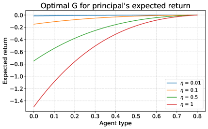
Figure 2: Principal’s expected financial return (16) from offering a separating menu rather than the base contract $(\tau_{\bar{q}},R_{\bar{q}},C_{\bar{q}})=(0.004,100,1.3)$ to each agent type. The separating menus are constructed using $\mathcal{G}$ from equation (18), where $\epsilon{(z)}=\eta\cdot(1-z)^{2}$ for the choices $\eta\in\{0.01,0.1,0.5,1\}$.

First, consider a type-dependent reward with the function $\mathcal{G}$ from equation (18), chosen to maximize the principal’s expected financial return. For illustration, we focus on an alternative with $\theta_{1}=1$. We consider a worst agent type with prior null probability $\bar{q}=0.8$ and use type-optimal thresholds (6) for FDR control. The false discovery rate is constrained at level $0.25$, which implies an optimal $p$-value threshold of $\tau_{\bar{q}}=0.004$ for this agent. The base contract fixes the reward at $R_{\bar{q}}=100$, with the cost $C_{\bar{q}}$ calibrated so that the worst type obtains zero utility under this contract.

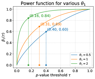
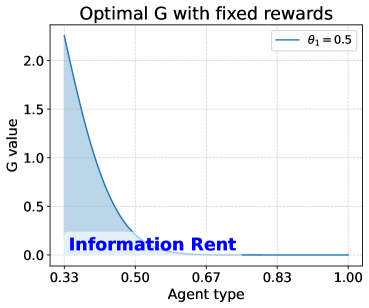
(a) $\beta_{1}(\tau)$		(b) $\theta_{1}=0.5$
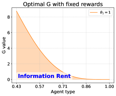
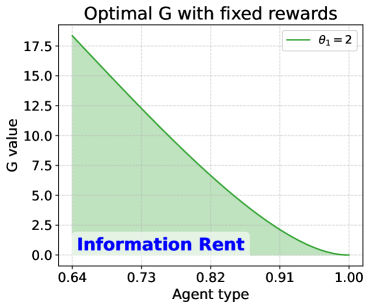
(c) $\theta_{1}=1$		(d) $\theta_{1}=2$

Figure 3: (a) Power functions $\beta_{1}(\tau)$ under alternative hypotheses $\theta_{1}\in\{0.5,1,2\}$, with the maximum threshold $\tau$ satisfying condition (19b) marked. (b)–(d) Plots of the function $\mathcal{G}$ from equation (21) under the same alternatives. The shaded area indicates the total information rent for uniformly distributed agent types under the separating menu constructed from $\mathcal{G}$.

As an illustration of the behavior of $\mathcal{G}$, we consider the perturbation function $\epsilon{(z)}:\,\!=\eta\cdot(1-z)^{2}$ for some $\eta>0$; in Figure 2, we plot the principal’s expected financial return (16), relative to the base contract, when using a separating menu constructed from $\mathcal{G}$ for the four choices $\eta\in\{0.01,0.1,0.5,1\}$. Here, the area under each curve represents the principal’s total financial loss for a population of agents with uniformly distributed types. Observe that setting $\eta$ close to zero results in smaller and smaller screening cost.

We next turn to the case of a constant reward across all contracts. We fix the reward at $100$ and again use type-optimal thresholds (6) with an FDR constraint at level $0.25$. As analyzed in (21), the function $\mathcal{G}$ now depends on the power function $\beta_{1}(\tau)$. We consider three different alternatives for the nonnull hypothesis: $\theta_{1}\in\{0.5,1,2\}$, with the null still given by $\theta_{0}=0$.

In Figure 3(a), we plot the power functions corresponding to these values of $\theta_{1}$, and mark the maximum $p$-value threshold for which the condition $\beta_{1}^{\prime}(\tau)>1$ from equation (19b) holds. As $\theta_{1}$ increases, the power function becomes steeper, and the maximum threshold satisfying this condition decreases. This restricts the range of agent types for whom contracts with constant reward are incentive-compatible. As discussed in Section 3.2.1, this maximum threshold imposes a lower bound on the agent types. The effect is exhibited in panels (b) through (d) of Figure 3, where we plot the corresponding functions $\mathcal{G}$. For example, when $\theta_{1}=0.5$, incentive-compatible contracts can be offered to agents with prior null beliefs in the interval $[0.33,1]$. As $\theta_{1}$ increases to 2, this range shifts toward agents with higher $q$, i.e., agents who are more likely to face the null hypothesis. This shift occurs because when $\theta_{1}=2$, the maximum separating threshold is approximately 0.16, which is too stringent to be optimal for agents with lower $q$. The shaded regions in panels (b)–(d) represent the total information rent incurred when offering the menu to a uniformly distributed population of agent types. As previously discussed, we see that a more powerful test increases the information rent required to screen better types.

4 Discussion

In this paper, we studied hypothesis testing over a heterogeneous population of strategic agents with private information. In this setting, any single uniform test yields sub-optimal performance, due to the underlying heterogeneity in agent types. At the other extreme, an oracle given a priori access to agent types can construct an optimal test for each type. Our main result was to show that it is possible for the principal to design a separating menu of type-tailored tests, coupled with appropriately designed payoffs, that induce agents to self-select according to their private information, thereby implementing type-optimal thresholds and achieving statistical efficiency. Strikingly, this improvement comes at negligible additional cost relative to single-test designs, demonstrating that information elicitation through incentive design can lead to better statistical performance with little cost.

Beyond the technical results specific to this paper, our analysis also offers some broader conceptual insights. First, it underscores the importance of treating agents as strategic and heterogeneous: conventional approaches that assume passive participants miss key opportunities for improving statistical outcomes. Second, it demonstrates how hypothesis tests themselves can serve as instruments of information elicitation. By embedding contracts in statistical design, the principal can shape agents’ utilities into a proper scoring rule, ensuring incentive compatibility. More broadly, the results further develop the connection between mechanism design and statistical decision-making and highlight that design in strategic settings requires jointly considering statistical objectives and agent behavior.

There are a number of natural extensions to the current analysis. First, we assumed that each agent’s private information is one-dimensional, summarizing only their belief about type. In practice, agents may hold richer, multi-dimensional information; for example, a researcher’s prior knowledge across multiple outcomes or a drug developer’s beliefs about several treatment effects. Second, the current analysis is predicated upon the principal knowing the test’s power function; it would be interesting to explore extensions involving partial knowledge. A final opportunity lies in the scope of design and behavior considered. We focused on $p$-value thresholds and binary participation, abstracting away other levers. In reality, a regulator may be able to influence sample sizes, stopping rules, or test statistics, while agents may strategically respond to these choices. Extending the analysis to such richer action spaces could capture a wider range of interactions.

Acknowledgements

This work was partially funded by NSF-DMS-2413875 to SB and MJW, and the Cecil H. Green Chair and Ford Professorship to MJW.

Appendix A Separating menus for discrete types

In this section, we present a simpler procedure for constructing separating menus when the population consists of a finite number $N\geq 2$ of agent types. This setting can be viewed as a special case of the general construction in Theorem 1, but here we provide a direct derivation based on an iterative argument. We first describe the procedure, then explain how it relates to the convex-function approach, and finally illustrate its properties with numerical examples.

Throughout, we assume that there are $N$ distinct agent types with ordered prior null probabilities $q_{1}<q_{2}<\dots<q_{N}$. For menu design, it suffices that the principal knows this support set $\operatorname{supp}(\mathbb{T})=\{q_{t}\}_{t=1}^{N}$, without needing to know the distribution $\mathbb{T}$ over these types. Importantly, the type of any individual agent remains private.

A.1 Iterative procedure for menu construction

We first set up the notation needed to describe our iterative procedure. To avoid double subscripts, we index the contract menu by the integer $t\in[N]:\,\!=\{1,\dots,N\}$, so that any menu takes the form $\mathscr{M}=\big\{(\tau_{t},R_{t},C_{t})\mid t\in[N]\big\}$. If an agent of type $q_{t}$ selects contract $t$, then the menu is incentive-compatible when $\varphi_{\mathscr{M}}(q_{t})=q_{t}$ for all $t$.

We now introduce an iterative procedure for designing a contract menu $\mathscr{M}$. For $t\in[N]$, define the scalars $\Delta_{t}:\,\!=\beta_{1}(\tau_{t})-\beta_{0}(\tau_{t})$, along with the intervals $\mathcal{I}_{t}:\,\!=[\ell_{t},r_{t}]$ with endpoints

$$\ell_{t} :\,\!=q_{t}\big[R_{t}\Delta_{t}-R_{t-1}\Delta_{t-1}\big]+\big[R_{t-1}\beta_{1}(\tau_{t-1})-R_{t}\beta_{1}(\tau_{t})+C_{t}\big],\quad\mbox{and}$$

$$r_{t} :\,\!=q_{t-1}\big[R_{t}\Delta_{t}-R_{t-1}\Delta_{t-1}\big]+\big[R_{t-1}\beta_{1}(\tau_{t-1})-R_{t}\beta_{1}(\tau_{t})+C_{t}\big].$$

The procedure takes as input the pair $(R_{N},C_{N})$, and a sequence $\{\epsilon{(t)}\}_{t=2}^{N}$ of strictly positive scalars, and constructs the menu $\{(\tau_{t},R_{t},C_{t}\}_{t=1}^{N}$ as follows:

1. For each $t\in[N]$, compute the type-optimal threshold $\tau_{q_{t}}$ and set $\tau_{t}\equiv\tau_{q_{t}}$.

2. In a backward recursion $t=N,N-1,\ldots,2$:

   $${\bf{Update:}}\quad R_{t-1}=R_{t}\frac{\Delta_{t}}{\Delta_{t-1}}+\epsilon{(t)},$$ (A22a)

   $${\bf{Choose:}}\quad C_{t-1}\in\big[\ell_{t},r_{t}\big].$$ (A22b)

The following proposition certifies when this procedure correctly computes a separating menu. In stating this result, it is helpful to adopt the notation $\operatorname{Util}(q;\tau,R,C)$ to track the explicit dependence of the utility function (2c) on the triple $(\tau,R,C)$.

Proposition 1.

Assume that initial reward-cost pair $(R_{N},C_{N})$ is chosen such that the participation constraint for agent type $q_{N}$ holds—viz.

$$\operatorname{Util}(q_{N};\tau_{N},R_{N},C_{N})\geq 0.$$ (A22c)

Then for any strictly positive sequence $\{\epsilon{(t)}\}_{t=2}^{N}$, the iterative procedure returns a contract menu $\mathscr{M}=\{(\tau_{t},R_{t},C_{t})\}_{t=1}^{N}$ that is separating.

See Section D.7 for the proof of this claim.

This iterative procedure can be understood as a discrete analogue of the general convex-function construction in Theorem 1. In the finite-type case, the separating menu induces a discrete convex function $\mathcal{G}$. Specifically, step (A22a) ensures $-R_{t-1}\Delta_{t-1}<-R_{t}\Delta_{t}$, so that the slope of the utility function strictly increases with type. Since the slope of the utility under contract $(\tau_{q},R_{q},C_{q})$ coincides with the subgradient of $\mathcal{G}$ at $q$, step (A22a) guarantees that $g^{*}_{q_{t-1}}<g^{*}_{q_{t}}$, yielding a sequence of increasing subgradients. Consequently, the truthful-reporting utility becomes convex in agent type. Step (A22b) then chooses the intercept to make the utility coincide with the supporting hyperplane of $\mathcal{G}$ at each type. In this way, the procedure constructs a discrete convex function satisfying property (10a), ensuring incentive compatibility. Condition (A22c) plays the role of (10b), guaranteeing participation for the worst type, and hence for all others. Finally, just as in the general construction, separating menus are not unique. The slack parameters ${\epsilon{(t)}}$ can be chosen arbitrarily (so long as they are positive), and whenever the interval $[\ell_{t},r_{t}]$ is non-degenerate, the cost $C_{t}$ can be varied. Thus there exists an infinite family of separating menus. In the next subsection, we illustrate how these choices affect the menus in numerical simulations.

A.2 Illustration with Gaussian mean testing

In this section, we illustrate the separating menu constructed from procedure (A22a)–(A22b) using the Gaussian mean testing setup from Section 3.3. Consider a binary test with null $\theta_{0}=0$ and $\theta_{1}=1$. We focus on a population consisting of $N=5$ agent types, with prior null probabilities $q$ ranging over the set $\operatorname{supp}(\mathbb{T})=\{0.3,0.4,0.5,0.6,0.7\}$. With a target false discovery rate $\alpha=0.25$, the type-optimal $p$-value thresholds computed from (6) are $\{0.74,0.38,0.18,0.07,0.02\}$. To ensure that the participation constraint (A22c) is satisfied for agent $N=5$ with $q=0.7$, we set the cost-reward pair $(C_{5},R_{5})=(5,100)$.

To visualize the resulting menu, we plot the maximum expected utility attainable by each type $q\in[0,1]$, along with the contract that delivers this utility. Since the menu is separating, the resulting utility envelope coincides with a piecewise convex function. Each linear segment corresponds to the utility function (2c) induced by a specific contract and the range of types it attracts. The five designed types are highlighted in the plots, showing the specific contract each selects.

Figure 4 makes explicit how the discrete construction connects to the general convex characterization. In one direction, the separating menu induces a discrete convex function $\mathcal{G}(q)$, represented by the five dots marking truthful-reporting utilities. The slope of the supporting line segment through each dot coincides with the subgradient of $\mathcal{G}$ at that type, which determines the utility available to all other types from the same contract. Convexity ensures that each type maximizes utility by reporting truthfully. Conversely, starting from this discrete convex function—or from the piecewise convex envelope—it is possible to reconstruct the separating menu, establishing the correspondence between discrete and general constructions.

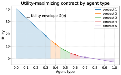
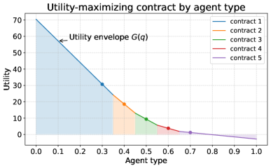
(a) $\epsilon{(t)}=50$		(b) $\epsilon{(t)}=100$
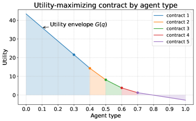
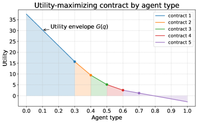
(c) $C_{t-1}$ close to the lower bound $\ell_{t}$		(d) $C_{t-1}$ close to the upper bound $r_{t}$

Figure 4: Plots of maximum utility (2c) achieved by each type $q\in[0,1]$ under a separating menu constructed for types $q\in\{0.3,0.4,0.5,0.6,0.7\}$. The dots mark the utilities of the designed types under truthful reporting, forming a discrete convex function $\mathcal{G}$. (a)-(b) Slack parameter $\epsilon{(t)}=50$ and $\epsilon{(t)}=100$, respectively, with $C_{t-1}=\frac{1}{2}[\ell_{t}+r_{t}]$. (c)-(d) Cost $C_{t-1}\approx\ell_{t}$ and $C_{t-1}\approx r_{t}$, respectively, with $\epsilon{(t)}=50$.

Figure 4 further illustrates how different choices of $\{\epsilon{(t)}\}_{t=2}^{N}$ and cost (A22b) affect the resulting menu. In panel (a), we set $\epsilon{(t)}=50$ for all $t\in\{2,\dots,5\}$; in panel (b), we increase this value to $\epsilon{(t)}=100$. In both cases, we set $C_{t-1}$ to the midpoint of the admissible interval $[\ell_{t},r_{t}]$ from equation (A22b). As we increase $\epsilon{(t)}$ from $50$ to $100$, we observe a more pronounced increase in the slope of the utility functions from contract 5 to contract 1. Intuitively, $\epsilon{(t)}$ controls the separation between types: larger values increase convexity of $\mathcal{G}$ and strengthen incentive compatibility.

In panel (c), we set $C_{t-1}$ to be the lower bound $\ell_{t-1}$ of the interval plus a small perturbation, while in panel (d), we set $C_{t-1}$ to be the upper bound $r_{t-1}$ minus a small perturbation, with both fixing $\epsilon{(t)}=50$ for all $t\in\{2,3,4,5\}$. Comparing panels (a), (c), and (d), we see that changing the choice of costs shifts the vertical intercept of the utility function induced by contract $t$. This shift then changes the location of the utility switch points—the values of $q$ at which an agent is indifferent between two adjacent contracts, i.e., where their expected utilities intersect. When $C_{t-1}$ is set near the lower bound of the interval, the switch point lies closer to type $q_{t}$, making contract $t$ nearly interchangeable with contract $t-1$ for that type. When $C_{t-1}$ is near the upper bound, the switch point moves toward $q_{t}$’s neighbor on the other side, making contract $t$ nearly interchangeable with contract $t+1$. Thus, the cost parameter effectively governs how the population is partitioned across adjacent contracts, while still preserving incentive compatibility.

Appendix B Separating menus under fixed costs

In this section, we show that constructing a separating menu in which all contracts share the same cost requires the power function to satisfy a form of convexity. We illustrate this in the simplest nontrivial setting with two agent types $q_{1}<q_{2}$ and corresponding type-optimal thresholds $\tau_{1}>\tau_{2}$.

Assume the base contract $(\tau_{2},R_{2},C_{2})$ is chosen so that the participation constraint (A22c) holds for type $q_{2}$. Following the procedure (A22a)–(A22b), the contract for type $q_{1}$ has reward

$$R_{1}=R_{2}\frac{\Delta_{2}}{\Delta_{1}}+\epsilon_{1}\qquad\mbox{for some}\quad\epsilon_{1}>0,$$ (A23)

where $\Delta_{t}=\beta_{1}(\tau_{t})-\beta_{0}(\tau_{t})$. Now suppose both contracts are constrained to have the same cost, i.e., $C_{1}=C_{2}=C$. For incentive compatibility, type $q_{2}$ must strictly prefer its designated contract over the alternative:

$$\operatorname{Util}(q_{2};\tau_{2},R_{2},C)>\operatorname{Util}(q_{2};\tau_{1},R_{1},C).$$

Substituting utility function (2c) and expression (A23) yields

$$R_{2}\big[q_{2}\beta_{0}(\tau_{2})+(1-q_{2})\beta_{1}(\tau_{2})\big]-C>\big[R_{2}\frac{\Delta_{2}}{\Delta_{1}}+\epsilon_{1}\big]\big[q_{2}\beta_{0}(\tau_{1})+(1-q_{2})\beta_{1}(\tau_{1})\big]-C.$$

Since $\epsilon_{1}>0$, this inequality implies that

$$\Delta_{1}\big[q_{2}\beta_{0}(\tau_{2})+(1-q_{2})\beta_{1}(\tau_{2})\big]>\Delta_{2}\big[q_{2}\beta_{0}(\tau_{1})+(1-q_{2})\beta_{1}(\tau_{1})\big],$$

which reduces to the following after simplification:

$$\beta_{0}(\tau_{2})\beta_{1}(\tau_{1})>\beta_{0}(\tau_{1})\beta_{1}(\tau_{2})$$

With $\beta_{0}(\tau)=\tau$, we conclude that for this fixed-cost menu to be incentive-compatible, the power function must satisfy

$$\frac{\beta_{1}(\tau_{1})}{\tau_{1}}>\frac{\beta_{1}(\tau_{2})}{\tau_{2}}\quad\mbox{for}\quad\tau_{1}>\tau_{2}.$$ (A24)

Inequality (A24) requires the ratio $\beta_{1}(\tau)/\tau$ to be strictly increasing in $\tau$. This property corresponds to the power function $\beta_{1}(\tau)$ being convex (or at least displaying convex-like curvature) on $[0,1]$. However, in most statistical settings, the power function of a test is concave in $\tau$: marginal increases in the significance level yield diminishing improvements in power. Under concavity, we have the opposite inequality—namely, $\frac{\beta_{1}(\tau_{1})}{\tau_{1}}\leq\frac{\beta_{1}(\tau_{2})}{\tau_{2}}$—which directly contradicts (A24).

Thus, a separating menu with constant costs can only exist if the power function is convex in $\tau$, a property rarely satisfied by common hypothesis tests. This explains why the constant-cost case is generally infeasible in practice, and motivates our focus on the constant-reward setting as the more realistic and broadly applicable case.

Appendix C Sensitivity to model misspecification

We have shown how to design separating menus that achieve statistical efficiency under the assumption that the principal knows the power function $\beta_{1}(\tau)$ precisely. In practice, however, it is often difficult to characterize the power function exactly. What then can be said about statistical efficiency in such cases? When $\beta_{1}(\tau)$ is entirely unknown, [SBW24] (Corollary 2) provides a worst-case bound on the false discovery rate induced by any statistical contract. This represents a pessimistic benchmark, reflecting the principal’s complete agnosticism about the power function.

More realistically, the principal may possess partial information, such as a set of plausible power functions—an assumption that naturally arises in simple-versus-composite testing problems. Such partial knowledge can support a more refined assessment of achievable statistical efficiency. In this section, we focus on a principal whose objective is to maximize TDR while controlling FDR at a prescribed level $\alpha$. We analyze the robustness of separating menus constructed under this criterion to misspecification of the power function, and in particular, how deviations from the assumed power function may lead to FDR violations for certain agent types.

FDR gap.

Suppose the principal constructs a separating menu using a power function $\beta_{1}(\tau)$, which determines the contract parameters $(\tau_{p},R_{p},C_{p})$. The type-optimal thresholds $\tau_{p}$ are chosen according to (6). However, an agent of type $q$ may hold beliefs aligned with a different power function $\tilde{\beta}_{1}(\tau)$. Recall that under the assumed power function $\beta_{1}(\tau)$, the menu is designed to control FDR for all reported types $p$:

$$\frac{p\beta_{0}(\tau_{p})}{p\beta_{0}(\tau_{p})+(1-p)\beta_{1}(\tau_{p})}=\frac{\beta_{0}(\tau_{p})}{\beta_{0}(\tau_{p})+\frac{(1-p)}{p}\beta_{1}(\tau_{p})}\leq\alpha.$$

In contrast, if the true power function is $\tilde{\beta}_{1}(\tau)$, the FDR incurred by an agent of type $q$ who reports $p$ becomes

$$\frac{q\beta_{0}(\tau_{p})}{q\beta_{0}(\tau_{p})+(1-q)\tilde{\beta}_{1}(\tau_{p})}=\frac{\beta_{0}(\tau_{p})}{\beta_{0}(\tau_{p})+\frac{(1-q)}{q}\tilde{\beta}_{1}(\tau_{p})}.$$

Hence, the sensitivity of FDR control to misspecification depends on the difference between the denominators in these two expressions. We define this difference as the FDR Gap:

$$\operatorname{FDR\ Gap}:\,\!=\frac{(1-p)}{p}\beta_{1}(\tau_{p})-\frac{(1-q)}{q}\tilde{\beta}_{1}(\tau_{p}).$$ (A25)

If $\operatorname{FDR\ Gap}\leq 0$, then even under misspecification, the FDR constraint continues to hold. If $\operatorname{FDR\ Gap}>0$, the constraint is violated, with the magnitude of the gap quantifying the degree of violation.

To evaluate the FDR gap (A25), the principal must determine which contract an agent of type $q$ selects. In general, obtaining a closed-form expression for the selection function (2a) under misspecification is challenging. To gain tractable insight, we analyze the special case of a fixed-reward separating menu constructed from $\mathcal{G}$ in (21). This setting allows us to characterize the factors that drive FDR violations. Under such a fixed-reward menu, if an agent with misspecified power function $\tilde{\beta}_{1}(\tau)$ reports type $p$, the resulting FDR gap is

$$\operatorname{FDR\ Gap}=\frac{(1-p)}{p}\beta_{1}(\tau_{p})-\frac{1-p}{p\big[1+\frac{\tilde{\beta}_{1}^{\prime}(\tau_{p})-\beta_{1}^{\prime}(\tau_{p})}{p\big(\beta_{1}^{\prime}(\tau_{p})-1\big)}\big]}\tilde{\beta}_{1}(\tau_{p}).$$ (A26)

See Section D.6 for a proof. Equation A26 highlights two main drivers of FDR sensitivity: (a) the difference in local slopes of the power functions, i.e., $\tilde{\beta}_{1}^{\prime}(\tau_{p})-\beta_{1}^{\prime}(\tau_{p})$, and (b) the value of $\tilde{\beta}_{1}(\tau_{p})$ itself. If the principal can restrict attention to a class of plausible power functions—such as in simple-versus-composite hypothesis testing—this characterization provides a concrete way to bound the extent of FDR violations arising from misspecification.

To obtain a concrete illustration, we examine the sensitivity of FDR control to misspecification in the setting of Gaussian mean testing. Following the setup in Section 3.3, we fix the reward at $100$ across all contracts and impose an FDR constraint of $0.25$. The separating menu is constructed under the assumption of a binary test with null hypothesis $\theta_{0}=0$ and alternative $\theta_{1}=1$. We consider $p$-value thresholds in the interval $[0.001,0.31]$, which corresponds to a separating menu for agents with $q\in[0.43,0.86]$.

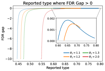
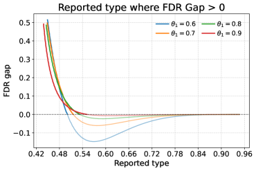
(a) $\tilde{\beta}_{1}(\tau)>\beta_{1}(\tau)$		(b) $\tilde{\beta}_{1}(\tau)<\beta_{1}(\tau)$

Figure 5: Plots of FDR gap (A26) as a function of the reported type $p$, using power function $\tilde{\beta}_{1}(\tau)$ under misspecified alternative hypotheses $\theta_{1}\neq 1$. (a) $\theta_{1}\in\{1.1,1.2,1.3,2\}$. (b) $\theta_{1}\in\{0.6,0.7,0.8,0.9\}$.

In Figure 5, we plot the FDR gap (A26) for various misspecified power functions. Panel (a) shows the case where $\tilde{\beta}_{1}(\tau)>\beta_{1}(\tau)$ with $\theta_{1}\in\{1.1,1.2,1.3,2\}$, while panel (b) considers $\tilde{\beta}_{1}(\tau)<\beta_{1}(\tau)$ with $\theta_{1}\in\{0.6,0.7,0.8,0.9\}$.

The results reveal a clear asymmetry. When the misspecified power function is overpowered, FDR violations arise primarily for contracts intended for agents with higher prior null. As shown in  Figure 5(a), for contracts associated with report types $p<0.6$, the FDR gap is negative and hence no violation occurs. A narrow band of mild violations emerges for $0.6<p<0.8$: for agents facing $\theta_{1}=1.1$ or $\theta_{1}=1.2$, the assigned thresholds $\tau_{p}$ can yield FDR violations, but the gap remains very small (upper bounded by $0.002$). By contrast, when the power function is underpowered, violations concentrate among contracts designed for agents with lower prior null. In Figure 5(b), the FDR gap is positive mainly for $p<0.55$. In summary, the FDR violation in this instance is negligible when the true $\theta_{1}$ is larger than the one used to construct the menu, whereas it can be large in the opposite case. This suggests that, in order to be robust, one should construct the menu with respect to the weakest plausible alternative—that is, the one yielding the lowest power.

Appendix D Proofs

In this section, we collect the proofs of our results.

D.1 Proof of Equation 2c

For notational simplicity, we introduce the shorthand $W:\,\!=R_{p}\>\mathbb{I}(X\leq\tau_{p})-C_{p}$, and note that $\operatorname{Util}(q,p)=\mathbb{E}[W]$ by definition. A simple calculation yields

$$\mathbb{E}[W] =q\mathbb{E}[W\mid\theta\in\Theta_{0}]+(1-q)\mathbb{E}[W\mid\theta\in\Theta_{1}]$$

$$=q\Big\{\mathbb{E}[W\mid\theta\in\Theta_{0}]-\mathbb{E}[W\mid\theta\in\Theta_{1}]\Big\}+\mathbb{E}[W\mid\theta\in\Theta_{1}].$$ (A27a)

Given the definition (2b) of the type I error $$\beta_{0}(\tau)$$, we can write

$$\mathbb{E}[W\mid\theta\in\Theta_{0}] =\beta_{0}(\tau_{p})\mathbb{E}[W\mid\theta\in\Theta_{0},X\leq\tau_{p}]+\big(1-\beta_{0}(\tau_{p})\big)\;\mathbb{E}[W\mid\theta\in\Theta_{0},X>\tau_{p}]$$

$$=\beta_{0}(\tau_{p})\big[R_{p}-C_{p}\big]-\big(1-\beta_{0}(\tau_{p})\big)C_{p}$$

$$=\beta_{0}(\tau_{p})R_{p}-C_{p}.$$ (A27b)

Similarly, the conditional expectation $$\mathbb{E}[W\mid\theta\in\Theta_{1}]$$ can be expressed as

$$\mathbb{E}[W\mid\theta\in\Theta_{1}] =\beta_{1}(\tau_{p})\mathbb{E}[W\mid\theta\in\Theta_{1},X\leq\tau_{p}]+\big(1-\beta_{1}(\tau_{p})\big)\;\mathbb{E}[W\mid\theta\in\Theta_{1},X>\tau_{p}]$$

$$=\beta_{1}(\tau_{p})R_{p}-C_{p}.$$ (A27c)

Combining equations (A27b) and (A27c) with the initial decomposition (A27a) yields

$$\operatorname{Util}(q,p)=\mathbb{E}[W]=qR_{p}\big[\beta_{0}(\tau_{p})-\beta_{1}(\tau_{p})\big]+\big[R_{p}\beta_{1}(\tau_{p})-C_{p}\big],$$

as claimed.

D.2 Proof of monotonicity of Equation 6

In this proof, we assume that $\tau_{q}>0$ as this is the only case relevant to menu construction. Recall that an agent of type $q$ who selects a $p$-value threshold $\tau$ incurs the FDR given by

$$\psi(q,\tau):\,\!=\frac{q\beta_{0}(\tau)}{q\beta_{0}(\tau)+(1-q)\beta_{1}(\tau)}.$$

To establish that the optimal threshold function $\tau_{q}$ is decreasing in the agent type $q$, it suffices to show that for any pair $q<\tilde{q}$, we have $\tau_{q}\geq\tau_{\tilde{q}}$, where

$$\tau_{q}=\sup\big\{\tau\,\mid\,\psi(q,\tau)\leq\alpha\big\}.$$

For agent type $\tilde{q}$, the optimal threshold $\tau_{\tilde{q}}$ satisfies that $\psi(\tilde{q},\tau_{\tilde{q}})\leq\alpha$. The key step, which we show later, is that the function $\psi(q,\tau)$ is strictly increasing in $q$:

$$\psi(q,\tau)<\psi(\tilde{q},\tau)\quad\mbox{for any $\tau>0$ and pair $q<\tilde{q}$.}$$ (A28)

This claim implies that $\psi(q,\tau_{\tilde{q}})<\psi(\tilde{q},\tau_{\tilde{q}})\leq\alpha$. By the definition of $\tau_{q}$ as the largest threshold satisfying the FDR constraint, we must have $\tau_{q}\geq\tau_{\tilde{q}}$.

Strict monotonicity:

When the power function $\beta_{1}(\tau)$ is concave and differentiable, the function $\psi(q,\tau)$ is also strictly increasing in $\tau$, a fact we will prove later:

$$\psi(q,\tau)<\psi(q,\tilde{\tau})\quad\mbox{for any $q>0$ and pair $0<\tau<\tilde{\tau}$.}$$ (A29)

Since $\psi(q,\tau_{\tilde{q}})<\psi(\tilde{q},\tau_{\tilde{q}})\leq\alpha$, inequality (A29) implies that $\tau_{q}>\tau_{\tilde{q}}$.

We now present the proofs of the two auxiliary claims stated earlier.

Proof of claim (A28):

Taking the derivative of $\psi(q,\tau)$ with respect to $q$ yields

$$\frac{d}{dq}\psi(q,\tau) =\frac{\big[q\beta_{0}(\tau)+(1-q)\beta_{1}(\tau)\big]\beta_{0}(\tau)-q\beta_{0}(\tau)\big[\beta_{0}(\tau)-\beta_{1}(\tau)\big]}{\big[q\beta_{0}(\tau)+(1-q)\beta_{1}(\tau)\big]^{2}}$$

$$=\frac{\beta_{0}(\tau)\beta_{1}(\tau)}{\big[q\beta_{0}(\tau)+(1-q)\beta_{1}(\tau)\big]^{2}},$$

which is strictly positive for $\tau>0$. Thus, $\psi$ is strictly increasing in $q$ for any fixed $\tau>0$ and we have established claim (A28).

Proof of claim (A29):

Differentiating the function $\psi(q,\tau)$ with respect to $\tau$ yields

$$\frac{d}{d\tau}\psi(q,\tau) =\frac{\big[q\beta_{0}(\tau)+(1-q)\beta_{1}(\tau)\big]q\beta_{0}^{\prime}(\tau)-q\beta_{0}(\tau)\big[\beta_{0}^{\prime}(\tau)-\beta_{1}^{\prime}(\tau)\big]}{\big[q\beta_{0}(\tau)+(1-q)\beta_{1}(\tau)\big]^{2}}$$

$$=\frac{q(1-q)\big[\beta_{0}^{\prime}(\tau)\beta_{1}(\tau)-\beta_{0}(\tau)\beta_{1}^{\prime}(\tau)\big]}{\big[q\beta_{0}(\tau)+(1-q)\beta_{1}(\tau)\big]^{2}}.$$

Since $\beta_{0}(\tau)=\tau$, we have $\beta_{0}^{\prime}(\tau)=1$. Assumption (8) implies that $\beta_{1}(\tau)$ is not linear function on $[0,1]$. The concavity of $\beta_{1}(\tau)$ then implies that

$$\beta_{1}^{\prime}(\tau)<\frac{\beta_{1}(\tau)-\beta_{1}(0)}{\tau}\quad\mbox{for all}\quad\tau>0,$$

which is equivalent to $\beta_{1}(\tau)-\tau\beta_{1}^{\prime}(\tau)>0$. Thus, $\frac{d}{d\tau}\psi(q,\tau)$ is strictly positive for $\tau>0$ and claim (A29) follows.

D.3 Proof of Theorem 1

We split the proof into two parts. The first part establishes the forward direction—namely, that any contract menu constructed according to the specified procedure is separating—while the second part proves the converse.

D.3.1 Forward direction

From the specification (11) of the reward $R_{p}$, the subgradient $g^{*}_{p}$ of the function $\mathcal{G}$ satisfies

$$g^{*}_{p}=R_{p}\big[\beta_{0}(\tau_{p})-\beta_{1}(\tau_{p})\big].$$ (A30)

The non-trivial power condition (8) combined with condition (10a) on $\mathcal{G}$ ensure that $R_{p}>0$ for all $p\in\operatorname{supp}(\mathbb{T})$.

Substituting the subgradient (A30) into expression (11) for the cost $C_{p}$ and rearranging yields

$$\mathcal{G}(p) =R_{p}\Big[p\beta_{0}(\tau_{p})+(1-p)\beta_{1}(\tau_{p})\Big]-C_{p}.$$

Thus, we see that the function value $\mathcal{G}(q)$ is exactly the utility (2c) of agent type $q$ under truthful reporting.

In order to establish that the constructed menu is separating, we need to show that

$$\operatorname{Util}(q;q) >\operatorname{Util}(q;p) \mbox{for all}\quad p,q\in\operatorname{supp}(\mathbb{T})\;\mbox{and}\;p\neq q,$$ (A31a)

$$\operatorname{Util}(q;q) \geq 0 \mbox{for all}\quad q\in\operatorname{supp}(\mathbb{T}).$$ (A31b)

Conditions (A31a) and (A31b) ensure that the menu is incentive-compatible and satisfies participation constraints, respectively.

Proof of condition (A31a).

By property (10a), for all $q\in\operatorname{supp}(\mathbb{T})$, we have

$$\mathcal{G}(q)>\mathcal{G}(p)+g^{*}_{p}(q-p)\qquad\mbox{for all $p\in\operatorname{supp}(\mathbb{T})\backslash\{q\}$.}$$

Substituting expression (A30) and the relation $\mathcal{G}(q)=\operatorname{Util}(q;q)$ yields

$$\operatorname{Util}(q;q)>\operatorname{Util}(p;p)+R_{p}\big[\beta_{0}(\tau_{p})-\beta_{1}(\tau_{p})\big](q-p)\qquad\mbox{for all $p\in\operatorname{supp}(\mathbb{T})\backslash\{q\}$.}$$

Plugging in definition (2c) for $\operatorname{Util}(p;p)$ and rearranging, we see that the right-hand side of this expression is equivalent to

$$\operatorname{Util}(p;p)+R_{p}\big[\beta_{0}(\tau_{p})-\beta_{1}(\tau_{p})\big](q-p)=R_{p}\big[q\beta_{0}(\tau_{p})+(1-q)\beta_{1}(\tau_{p})\big]-C_{p}=\operatorname{Util}(q;p).$$ (A32)

Combining the pieces, we conclude that $\operatorname{Util}(q;q)>\operatorname{Util}(q;p)$.

Proof of condition (A31b).

By property (10b), we are guaranteed to have

$$\mathcal{G}(\bar{q})=\operatorname{Util}(\bar{q};\bar{q})\geq 0\qquad\mbox{where $\bar{q}=\sup\{q\mid q\in\operatorname{supp}(\mathbb{T})\}$.}$$

Therefore, condition (A31b) holds for $\bar{q}$. Condition (A31a) implies that $\mathcal{G}(q)=\operatorname{Util}(q;q)>\operatorname{Util}(q;\bar{q})$ for all $q<\bar{q}$. Based on the discussion around Equation 2c, the function $q\mapsto\operatorname{Util}(q;p)$ is strictly decreasing, which implies that $\operatorname{Util}(q;\bar{q})>\operatorname{Util}(\bar{q};\bar{q})$ for all $q<\bar{q}$. Chaining these inequalities yields that $\mathcal{G}(q)>\mathcal{G}(\bar{q})\geq 0$ for all $q<\bar{q}$.

D.3.2 The converse

Consider a separating menu $(\tau_{p},R_{p},C_{p})$ indexed by agent types $q\in\operatorname{supp}(\mathbb{T})$. We now show that it can be associated with a function $\mathcal{G}$ that satisfies conditions (10a) and (10b). In particular, recalling the utility function (2c), we define $\mathcal{G}(q):\,\!=\operatorname{Util}(q;q)$, which is the utility attained by each agent type under truthful reporting. Moreover, we define the scalars

$$g^{*}_{q}:\,\!=R_{q}\big[\beta_{0}(\tau_{q})-\beta_{1}(\tau_{q})\big]\quad\mbox{for each $q\in\operatorname{supp}(\mathbb{T})$.}$$ (A33)

Proof of property (10a).

Since the menu is incentive-compatible, by condition (A31a), we know

$$\operatorname{Util}(q;q)>\operatorname{Util}(q;p)\quad\mbox{for all}\quad p,q\in\operatorname{supp}(\mathbb{T})\;\mbox{and}\;p\neq q.$$

The equivalent expression in equation (A32) implies that

$$\operatorname{Util}(q;q)>\operatorname{Util}(p;p)+R_{p}\big[\beta_{0}(\tau_{p})-\beta_{1}(\tau_{p})\big](q-p).$$

Equivalently, using the definition (A33), we have

$$\mathcal{G}(q)>\mathcal{G}(p)+g^{*}_{p}(q-p)\quad\mbox{for all}\quad q\in\operatorname{supp}(\mathbb{T}).$$

Moreover, definition (A33) combined with the non-trivial power assumption (8) implies that $g^{*}_{p}<0$. Therefore, we conclude that property (10a) holds.

Proof of property (10b).

Since the menu satisfies the participation constraint (A31b), we have $\mathcal{G}(q)=\operatorname{Util}(q;q)\geq 0$ for all $q\in\operatorname{supp}(\mathbb{T})$. Property (10b) thus holds immediately.

D.4 Proof of Corollary 2

In order to show that the menu is separating using Theorem 1, it suffices to show that the function $\mathcal{G}$ from equation (18) satisfies properties (10a) and (10b). By the non-trivial power assumption (8), we have $\beta_{0}(\tau)-\beta_{1}(\tau)<0$. From the definition (18), we see that $\mathcal{G}$ is differentiable with derivative

$$\underbrace{\mathcal{G}^{\prime}(q)}_{\equiv g^{*}_{q}}=R_{\bar{q}}\big[\beta_{0}(\tau_{\bar{q}})-\beta_{1}(\tau_{\bar{q}})\big](1+\epsilon{(q)}).$$

Since $\epsilon{(q)}\geq 0$, it follows that $g^{*}_{q}<0$. Moreover, because the mapping $q\mapsto\epsilon{(q)}$ is differentiable, the second derivative of $\mathcal{G}$ is given by

$$\mathcal{G}^{\prime\prime}(q)=\frac{d}{dq}\mathcal{G}^{\prime}(q)=R_{\bar{q}}\big[\beta_{0}(\tau_{\bar{q}})-\beta_{1}(\tau_{\bar{q}})\big]\epsilon^{\prime}(q).$$

Since $\epsilon^{\prime}(q)<0$, we have $\mathcal{G}^{\prime\prime}(q)>0$, implying that $\mathcal{G}$ is strictly convex on $[0,\bar{q}]$. Thus, we conclude that $\mathcal{G}$ satisfies property (10a). Finally, by assumption (15), we have $\mathcal{G}(\bar{q})=0$, verifying the second condition (10b).

Next, we argue that the principal can make the screening cost (14) arbitrarily small by adjusting the values $\epsilon{(z)}$. It suffices to verify this for a single agent type $q$, whose screening cost under (18) is given by

$$\Bigg\{R_{\bar{q}}\big[\beta_{1}(\tau_{\bar{q}})-\beta_{0}(\tau_{\bar{q}})\big]\int_{q}^{\bar{q}}\big[1+\epsilon{(z)}\big]dz\Bigg\}-\Bigg\{qR_{\bar{q}}\big[\beta_{0}(\tau_{\bar{q}})-\beta_{1}(\tau_{\bar{q}})\big]+\big[R_{\bar{q}}\beta_{1}(\tau_{\bar{q}})-C_{\bar{q}}\big]\Bigg\}.$$

Rearranging terms, we obtain

$$-\bigg\{R_{\bar{q}}\big[\beta_{0}(\tau_{\bar{q}})-\beta_{1}(\tau_{\bar{q}})\big]\bigg(\bar{q}+\int_{q}^{\bar{q}}\epsilon{(z)}dz\bigg)+\big[R_{\bar{q}}\beta_{1}(\tau_{\bar{q}})-C_{\bar{q}}\big]\bigg\}.$$

As $\epsilon{(z)}\rightarrow 0^{+}$, the integral $\int_{q}^{\bar{q}}\epsilon{(z)}dz$ converges to zero. Consequently, the screening cost can be made arbitrarily close to $-\operatorname{Util}(\bar{q};\tau_{\bar{q}},R_{\bar{q}},C_{\bar{q}})$. This proves the claim, since $\operatorname{Util}(\bar{q};\tau_{\bar{q}},R_{\bar{q}},C_{\bar{q}})=0$ by assumption (15).

D.5 Proof of Corollary 3

In order to show that the menu is separating using Theorem 1, it suffices to show that the function $\mathcal{G}$ from equation (21) satisfies properties (10a) and (10b). From its definition (21), the function $\mathcal{G}$ is differentiable with derivative $\mathcal{G}^{\prime}(q)=R\big[\beta_{0}(\tau_{q})-\beta_{1}(\tau_{q})\big]$. By the non-trivial power assumption (8) and the fact that $R>0$, it follows that $\mathcal{G}^{\prime}(q)\equiv g^{*}_{q}<0$.

Since $\beta_{1}(\tau)$ is concave and differentiable, the second derivative of $\mathcal{G}$ is given by

$$\mathcal{G}^{\prime\prime}(q)=R\big[\beta_{0}^{\prime}(\tau_{q})\tau^{\prime}_{q}-\beta_{1}^{\prime}(\tau_{q})\tau^{\prime}_{q}\big]\stackrel{{\scriptstyle(i)}}{{=}}R\big[1-\beta_{1}^{\prime}(\tau_{q})\big]\tau^{\prime}_{q},$$

where step (i) uses the identity $\beta_{0}(\tau)=\tau$ and the fact that $\beta_{0}^{\prime}(\tau)=1$. By assumption (19c), we have $\tau^{\prime}_{q}<0$. Combined with condition (19b), this implies that $\mathcal{G}^{\prime\prime}(q)>0$ and thus $\mathcal{G}$ is strictly convex on $[\underline{q},\bar{q}]$. It follows that property (10a) holds. Finally, assumption (15) implies that $\mathcal{G}(\bar{q})=0$, verifying property (10b).

Because $\mathcal{G}$ is differentiable and its derivative is specified everywhere, the function is determined up to an additive constant. The condition $\mathcal{G}(\bar{q})=0$ removes this indeterminacy, yielding a unique function $\mathcal{G}$. Through the correspondence in Theorem 1, we conclude that the separating menu under fixed reward is uniquely determined.

D.6 Proof of Equation A26

Under a fixed-reward separating menu, the selection function for an agent of type $q$ with misspecified power function $\tilde{\beta}_{1}(\cdot)$ is

$$\varphi_{\mathscr{M}}(q) =\arg\max_{p\in\mathcal{P}}\operatorname{Util}(q;p)\;=\;\arg\max_{p\in\mathcal{P}}R\big[q\beta_{0}(\tau_{p})+(1-q)\tilde{\beta}_{1}(\tau_{p})\big]-C_{p},$$ (A34)

where $C_{p}$ is given by (20). Differentiating the objective in (A34) with respect to $p$ and setting the derivative to zero yields

$$R\tau^{\prime}_{p}\big[q\beta_{0}^{\prime}(\tau_{p})+(1-q)\tilde{\beta}_{1}^{\prime}(\tau_{p})\big]=R\tau^{\prime}_{p}\big[p\beta_{0}^{\prime}(\tau_{p})+(1-p)\beta_{1}^{\prime}(\tau_{p})\big].$$

Cancelling $R\tau^{\prime}_{p}$ from both sides and rearranging gives the condition that the reported type $p$ must satisfy:

$$q\beta_{0}^{\prime}(\tau_{p})+(1-q)\tilde{\beta}_{1}^{\prime}(\tau_{p})=p\beta_{0}^{\prime}(\tau_{p})+(1-p)\beta_{1}^{\prime}(\tau_{p}).$$

Solving for $q$ in terms of $p$ gives $q=\frac{p\beta_{0}^{\prime}(\tau_{p})+(1-p)\beta_{1}^{\prime}(\tau_{p})-\tilde{\beta}_{1}^{\prime}(\tau_{p})}{\beta_{0}^{\prime}(\tau_{p})-\beta_{1}^{\prime}(\tau_{p})}$. Finally, substituting this expression into the definition of the FDR gap (A25), and using the fact that $\beta_{0}^{\prime}(\tau_{p})=1$, establishes claim (A26).

D.7 Proof of Proposition 1

Here we analyze the iterative procedure for constructing a separating contract menu for finitely many agent types, as stated in Proposition 1.

D.7.1 Main argument

The recursive structure of the menu construction ensures that local incentive compatibility between adjacent types suffices to guarantee global truth-telling across all types. Accordingly, the bulk of our effort is devoted to analyzing incentive compatibility between adjacent types. In particular, we begin by stating two auxiliary lemmas that play a key role in the proof.

Our first lemma establishes conditions on rewards and costs that ensure incentive compatibility between a pair of adjacent types. Concretely, consider two adjacent agent types $q_{t}$ and $q_{t-1}$ with $q_{t-1}<q_{t}$, and type-optimal thresholds $\tau_{t}$ and $\tau_{t-1}$. Lemma 1 specifies conditions on the reward-cost pairs that ensure local incentive compatibility of the contracts $(\tau_{t},R_{t},C_{t})$ and $(\tau_{t-1},R_{t-1},C_{t-1})$.

Lemma 1.

The recursive construction (A22a) and (A22b) of reward-cost pairs ensures local incentive compatibility, meaning that

$$\operatorname{Util}(;\tau_{t-1},R_{t-1},C_{t-1})-\operatorname{Util}(;\tau_{t},R_{t},C_{t})>0,$$ (A35a)

$$\operatorname{Util}(;\tau_{t},R_{t},C_{t})-\operatorname{Util}(;\tau_{t-1},R_{t-1},C_{t-1})>0.$$ (A35b)

See Section D.7.2 for the proof.

Our second lemma formalizes an important type of monotonic preference structure in the contracts, ensuring that no agent prefers a contract intended for a more distant type.

Lemma 2.

The contracts in any menu constructed by the iterative procedure satisfy the properties

$$\operatorname{Util}(q;\tau_{t},R_{t},C_{t}) >\operatorname{Util}(q;\tau_{t-1},R_{t-1},C_{t-1})\quad\mbox{for all}\quad q\geq,$$ (A36a)

$$\operatorname{Util}(q;\tau_{t},R_{t},C_{t}) <\operatorname{Util}(q;\tau_{t-1},R_{t-1},C_{t-1})\quad\mbox{for all}\quad q\leq.$$ (A36b)

See Section D.7.3 for the proof.

With these two lemmas in place, we are now prepared to prove the proposition itself. Lemma 1 ensures that any pair of adjacent contracts is locally incentive-compatible. Our first step is to leverage this property so as to establish global incentive compatibility, meaning that for each $t\in[N]$, we have

$$\operatorname{Util}(;\tau_{t},R_{t},C_{t})>\operatorname{Util}(;\tau_{s},R_{s},C_{s})\quad\mbox{for all}\quad s\in[N]\backslash\{t\}.$$ (A37)

To establish this property, first consider some $s\leq t$ and hence the contract $(\tau_{s},R_{s},C_{s})$ intended for $q_{s}\leq q_{t}$. Equation (A36a) from Lemma 2 implies that for agent type $q_{t}$,

$$\operatorname{Util}(;\tau_{s},R_{s},C_{s})>\operatorname{Util}(;\tau_{s-1},R_{s-1},C_{s-1}).$$

Chaining together relations of this type yields

$$\operatorname{Util}(;\tau_{t},R_{t},C_{t})>\operatorname{Util}(;\tau_{s},R_{s},C_{s})\quad\mbox{for all}\quad s<t.$$

Similarly, for any $s>t$, inequality (A36b) from Lemma 2 implies that for agent type $q_{t}$,

$$\operatorname{Util}(;\tau_{s-1},R_{s-1},C_{s-1})>\operatorname{Util}(;\tau_{s},R_{s},C_{s}).$$

Chaining these relations yields

$$\operatorname{Util}(;\tau_{t},R_{t},C_{t})>\operatorname{Util}(;\tau_{s},R_{s},C_{s})\quad\mbox{for all}\quad s>t.$$

Thus, the global incentive compatibility constraint is satisfied for each agent type.

Now, we show that the constructed menu satisfies the participation constraints, i.e., for each agent of type , we have $\operatorname{Util}(;\tau_{t},R_{t},C_{t})\geq 0$. By assumption, this inequality holds trivially for agent type . For any $t<N$, by the incentive compatibility constraints, we have

$$\operatorname{Util}(;\tau_{t},R_{t},C_{t})>\operatorname{Util}(;\tau_{N},R_{N},C_{N}).$$

Since $<$ for all $t<N$ and the function $q\mapsto\operatorname{Util}(q;\tau_{N},R_{N},C_{N})$ is monotonically decreasing in $q$, we have

$$\operatorname{Util}(;\tau_{N},R_{N},C_{N})>\operatorname{Util}(;\tau_{N},R_{N},C_{N})\geq 0.$$

Consequently, we conclude that $\operatorname{Util}(;\tau_{t},R_{t},C_{t})\geq 0$ for all $t<N$, as claimed.

D.7.2 Proof of Lemma 1

Recalling the shorthand $\Delta_{t}:\,\!=\beta_{1}(\tau_{t})-\beta_{0}(\tau_{t})$, the utility function (2c) takes the form

$$\operatorname{Util}(q;\tau_{t},R_{t},C_{t}) =-qR_{t}\Delta_{t}+\big[R_{t}\beta_{1}(\tau_{t})-C_{t}\big].$$

We substitute this utility function into equations (A35a) and (A35b); by re-arranging, we find that the cost $C_{t-1}$ must satisfy the upper and lower bounds

$$C_{t-1} <r_{t}:\,\!=\Big(R_{t}\Delta_{t}-R_{t-1}\Delta_{t-1}\Big)+\Big[R_{t-1}\beta_{1}(\tau_{t-1})-R_{t}\beta_{1}(\tau_{t})+C_{t}\Big],\quad\mbox{and}$$

$$C_{t-1} >\ell_{t}:\,\!=\Big(R_{t}\Delta_{t}-R_{t-1}\Delta_{t-1}\Big)+\Big[R_{t-1}\beta_{1}(\tau_{t-1})-R_{t}\beta_{1}(\tau_{t})+C_{t}\Big].$$

In order to guarantee the existence of such $C_{t-1}$, we require

$$\Big(R_{t}\Delta_{t}-R_{t-1}\Delta_{t-1}\Big)>\Big(R_{t}\Delta_{t}-R_{t-1}\Delta_{t-1}\Big).$$

Since $>$, this condition can be satisfied by requiring that

$$R_{t}\Delta_{t}-R_{t-1}\Delta_{t-1}<0.$$ (A39)

Recall that our non-trivial power assumption ensures that $\beta_{1}(\tau)>\beta_{0}(\tau)$ for all $\tau\in[0,1]$; as a consequence, we have $\Delta_{t}>0$ and $\Delta_{t-1}>0$. Re-arranging yields the equivalent inequality $R_{t-1}>R_{t}\frac{\Delta_{t}}{\Delta_{t-1}}$, which is satisfied by setting

$$R_{t-1}=R_{t}\frac{\Delta_{t}}{\Delta_{t-1}}+\epsilon{(t)}\qquad\mbox{for some $\epsilon{(t)}>0$.}$$

This completes the proof.

D.7.3 Proof of Lemma 2

Recall that the expected utility function $q\mapsto\operatorname{Util}(q;\tau_{t},R_{t},C_{t})$ is linear in $q$ and has a negative slope $-R_{t}\Delta_{t}$. Lemma 1 ensures that $-R_{t}\Delta_{t}>-R_{t-1}\Delta_{t-1}$. Using the linear structure, we can write

$$\operatorname{Util}(q;\tau_{t},R_{t},C_{t}) =\operatorname{Util}(;\tau_{t},R_{t},C_{t})-(q-)R_{t}\Delta_{t}$$

$$\operatorname{Util}(q;\tau_{t-1},R_{t-1},C_{t-1}) =\operatorname{Util}(;\tau_{t-1},R_{t-1},C_{t-1})-(q-)R_{t-1}\Delta_{t-1}$$

Now for any prior null probability $q\geq$, we have

$$-(q-)R_{t}\Delta_{t}>-(q-)R_{t-1}\Delta_{t-1}.$$

Given incentive compatibility, i.e., $\operatorname{Util}(;\tau_{t},R_{t},C_{t})>\operatorname{Util}(;\tau_{t-1},R_{t-1},C_{t-1})$, we conclude that

$$\operatorname{Util}(q;\tau_{t},R_{t},C_{t})>\operatorname{Util}(q;\tau_{t-1},R_{t-1},C_{t-1})\quad\mbox{for all}\quad q\geq.$$

The proof of equation A36b is similar. Using the linear structure, we can write

$$\operatorname{Util}(q;\tau_{t},R_{t},C_{t}) =\operatorname{Util}(;\tau_{t},R_{t},C_{t})-(q-)R_{t}\Delta_{t}$$

$$\operatorname{Util}(q;\tau_{t-1},R_{t-1},C_{t-1}) =\operatorname{Util}(;\tau_{t-1},R_{t-1},C_{t-1})-(q-)R_{t-1}\Delta_{t-1}$$

For all $q\leq$, we have $-(q-)R_{t}\Delta_{t}<-(q-)R_{t-1}\Delta_{t-1}$. Combining this inequality with incentive compatibility yields

$$\operatorname{Util}(q;\tau_{t},R_{t},C_{t})<\operatorname{Util}(q;\tau_{t-1},R_{t-1},C_{t-1})\quad\mbox{for all}\quad q\leq,$$

which completes the proof.

References

- [Bat+22] Stephen Bates, Michael I. Jordan, Michael Sklar and Jake A. Soloff “Principal-Agent Hypothesis Testing” In arXiv preprint arXiv:2205.06812, 2022 arXiv:2205.06812 [cs.GT]
- [Bat+23] Stephen Bates, Michael I. Jordan, Michael Sklar and Jake A. Soloff “Incentive-Theoretic Bayesian Inference for Collaborative Science” In arXiv preprint arXiv:2307.03748, 2023 arXiv:2307.03748 [stat.ME]
- [BD04] Patrick Bolton and Mathias Dewatripont “Contract Theory” MIT Press, 2004
- [Ber+13] Richard Berk et al. “Valid post-selection inference” In The Annals of Statistics, 2013, pp. 802–837
- [BM82] David P Baron and Roger B Myerson “Regulating a monopolist with unknown costs” In Econometrica: Journal of the Econometric Society JSTOR, 1982, pp. 911–930
- [Bri50] Glenn W Brier “Verification of forecasts expressed in terms of probability” In Monthly weather review 78.1, 1950, pp. 1–3
- [Che+18] Yiling Chen, Chara Podimata, Ariel D Procaccia and Nisarg Shah “Strategyproof linear regression in high dimensions” In Proceedings of the 2018 ACM Conference on Economics and Computation, 2018, pp. 9–26
- [CL06] T. Tony Cai and Mark G. Low “Optimal adaptive estimation of a quadratic functional” In Annals of Statistics 34.5, 2006, pp. 2298–2325 DOI: 10.1214/009053606000000849
- [DFP10] Ofer Dekel, Felix Fischer and Ariel D Procaccia “Incentive compatible regression learning” In Journal of Computer and System Sciences 76.8 Elsevier, 2010, pp. 759–777
- [Don+18] Jinshuo Dong et al. “Strategic classification from revealed preferences” In Proceedings of the 2018 ACM Conference on Economics and Computation, 2018, pp. 55–70
- [Goo52] Irving John Good “Rational decisions” In Journal of the Royal Statistical Society: Series B (Methodological) 14.1 Wiley Online Library, 1952, pp. 107–114
- [GR07] Tilmann Gneiting and Adrian E Raftery “Strictly proper scoring rules, prediction, and estimation” In Journal of the American statistical Association 102.477 Taylor & Francis, 2007, pp. 359–378
- [Har+16] Moritz Hardt, Nimrod Megiddo, Christos Papadimitriou and Mary Wootters “Strategic classification” In Proceedings of the 2016 ACM conference on innovations in theoretical computer science, 2016, pp. 111–122
- [HCC25] Safwan Hossain, Yatong Chen and Yiling Chen “Strategic Hypothesis Testing”, 2025 arXiv: https://arxiv.org/abs/2508.03289
- [JV25] Ravi Jagadeesan and Davide Viviano “Publication Design with Incentives in Mind” In arXiv preprint arXiv:2504.21156, 2025
- [Lep90] Oleg V. Lepski “A problem of adaptive estimation in Gaussian white noise” In Theory of Probability and Its Applications 35.3, 1990, pp. 454–466
- [LM01] Jean-Jacques Laffont and David Martimort “The Theory of Incentives: The Principal-Agent Model” Princeton, NJ, USA: Princeton University Press, 2001
- [LT93] Jean-Jacques Laffont and Jean Tirole “A theory of incentives in procurement and regulation” MIT press, 1993
- [McC56] John McCarthy “Measures of the value of information” In Proceedings of the National Academy of Sciences 42.9, 1956, pp. 654–655
- [MM24] Adam McCloskey and Pascal Michaillat “Critical Values Robust to P-hacking” In The Review of Economics and Statistics, 2024, pp. 1–35 DOI: 10.1162/rest˙a˙01456
- [MR78] Michael Mussa and Sherwin Rosen “Monopoly and product quality” In Journal of Economic theory 18.2 Academic Press, 1978, pp. 301–317
- [MR84] Eric Maskin and John Riley “Monopoly with incomplete information” In The RAND Journal of Economics 15.2 JSTOR, 1984, pp. 171–196
- [MR84a] Eric Maskin and John Riley “Optimal auctions with risk averse buyers” In Econometrica: Journal of the Econometric Society JSTOR, 1984, pp. 1473–1518
- [Mye81] Roger B Myerson “Optimal auction design” In Mathematics of operations research 6.1 INFORMS, 1981, pp. 58–73
- [PPP04] Javier Perote and Juan Perote-Pena “Strategy-proof estimators for simple regression” In Mathematical Social Sciences 47.2 Elsevier, 2004, pp. 153–176
- [Sal05] Bernard Salanie “The Economics of Contracts: A Primer, 2nd Edition” MIT Press, 2005
- [Sav71] Leonard J Savage “Elicitation of personal probabilities and expectations” In Journal of the American Statistical Association 66.336 Taylor & Francis, 1971, pp. 783–801
- [SBW24] Flora C Shi, Stephen Bates and Martin J Wainwright “Sharp Results for Hypothesis Testing with Risk-Sensitive Agents” In arXiv preprint arXiv:2412.16452, 2024
- [Spi18] Jann Spiess “Optimal estimation when researcher and social preferences are misaligned” Working paper, 2018 URL: https://gsb-faculty.stanford.edu/jann-spiess/files/2021/01/alignedestimation.pdf
- [Spo96] Vladimir Spokoiny “Adaptive hypothesis testing using wavelets” In Annals of Statistics 24.6, 1996, pp. 2477–2498
- [Tet16] Aleksey Tetenov “An economic theory of statistical testing”, 2016
- [TT15] Jonathan Taylor and Robert J Tibshirani “Statistical learning and selective inference” In Proceedings of the National Academy of Sciences 112.25 National Acad Sciences, 2015, pp. 7629–7634
- [VWN24] Davide Viviano, Kaspar Wuthrich and Paul Niehaus “A model of multiple hypothesis testing”, 2024 arXiv: https://arxiv.org/abs/2104.13367
- [Wan23] Han Wang “Contracting with Heterogeneous Researchers”, 2023 arXiv: https://arxiv.org/abs/2307.07629
- [WY25] Cole Wittbrodt and Nathan Yoder “Delegating Experiments” In Available at SSRN 5221631, 2025
- [Yod22] Nathan Yoder “Designing incentives for heterogeneous researchers” In Journal of Political Economy 130.8 The University of Chicago Press Chicago, IL, 2022, pp. 2018–2054