Mitigating Model Drift in Developing Economies
using Synthetic Data and Outliers

Abstract

Machine learning models in finance are highly susceptible to model drift, where predictive performance declines as data distributions shift. This issue is especially acute in developing economies such as those in Central Asia and the Caucasus—including Tajikistan, Uzbekistan, Kazakhstan, and Azerbaijan—where frequent and unpredictable macroeconomic shocks destabilize financial data. To the best of our knowledge, this is among the first studies to examine drift mitigation methods on financial datasets from these regions. We investigate the use of synthetic outliers, a largely unexplored approach, to improve model stability against unforeseen shocks. To evaluate effectiveness, we introduce a two-level framework that measures both the extent of performance degradation and the severity of shocks. Our experiments on macroeconomic tabular datasets show that adding a small proportion of synthetic outliers generally improves stability compared to baseline models, though the optimal amount varies by dataset and model.

1 Introduction

Machine learning models deployed in finance frequently experience performance degradation under distribution shift, known as model drift. Drift arises when statistical properties of new data diverge from the training distribution. More concretely, when the conditional relationship between features and outcomes changes, this is referred to as concept drift Hinder2024 ; Halstead2022 , and is particularly relevant in more unstable economies.

Traditional approaches to mitigating drift include monitoring model metrics and retraining with online or incremental learning, or expanding ensembles when drift is detected Gemaque2020 . Data-centric strategies such as resampling, sliding windows (keeping only the most recent chunk of data), domain adaptation to shifted distributions, and continuous feedback loops are also common Hinder2024 ; Gama2014 , as later discussed in Section 2. More recently, by simulating future distributions, synthetic data generation has been used to prepare models for drift conditions without waiting for real-world data Chiu2024 . However, the role of synthetic outliers in stabilizing models remains largely unexplored kraus2025machine particularly in the context of developing economies.

Building on this line of research, this paper makes the following contributions: (1) Stability metrics for model drift evaluation under shocks. We propose a two-level framework: the Stabilization Score (SS), which calculates the relative performance drop of a model under sudden shocks while normalizing by covariate drift, and the Stabilization Uplift (SU), a comparative evaluation of two models under shock, using their pre-/post-shock performance. (2) Synthetic outliers for model drift mitigation. We show that deliberately generated outliers, produced with zGAN azimi2024zgan , which we review in Appendix A, can improve model stability when combined with real and synthetic data (we calculate this using our metrics). (3) Focus on developing economies. While most work on model drift and stability relies on datasets from mature financial markets, we conduct experiments on macroeconomic tabular datasets from developing economies in Central Asia and the Caucasus, where shocks are often more present. This is both an underexplored empirical setting in the generative AI for finance literature and one where stabilization methods are especially critical.

We clarify the distinction between generic synthetic data and synthetic outliers in Appendix A, show the experimental pipeline in Appendix B, and provide shock origins and split types in Appendix C.

2 Related Work

Drift detection and adaptation methods. Several forms of drift are especially present in financial applications: time-based drift, where dependencies evolve gradually over time (e.g., seasonal repayment behavior in credit scoring Zliobaite2012 ); conditional drift, where new data arrives from underrepresented regions of the feature space (e.g., new geographies Gama2014 ); and contextual or sudden drift, where input–output relations shift abruptly due to external shocks such as pandemics, conflicts, or policy changes Tsymbal2004 . A central challenge is identifying when model performance deteriorates due to distributional change. The ADWIN (ADaptive WINdowing) algorithm Bifet2007 remains a widely used baseline that resizes its window based on detected change. More recent work considers stability under adversarial conditions Korycki_2022 , causal approaches for interpretability YANG2025 , practical case studies (e.g., COVID-19) highlighting the vulnerability of financial models to sudden shocks SONNLEITNER2025 , and applications in business processes kraus2025machine . Classical approaches rely on incremental or online learning with sliding/expanding windows Agrahari2024 ; neural models under continuously evolving distributions often employ statistical tests such as Kolmogorov–Smirnov (KS) Prashanth2025 ; and unsupervised settings benchmark drift detection on complex real-world data streams lukats2025benchmark .

Synthetic data. While the targeted use of synthetic outliers to mitigate drift and improve stability remains largely unexplored, related work includes Puranik et al. Puranik2024 , who propose the TabOOD framework to generate out-of-distribution tabular samples that improve generalization, and Kraus et al. kraus2025machine , who demonstrate the use of synthetic data for drift detection in business processes.

3 Stabilization Metrics for Model Drift Evaluation under Shocks

Shocks

We define a shock as a sudden, isolated event in the data-generating process or external conditions that causes an immediate and significant change in feature distributions. Shocks are so abrupt that the detailed temporal evolution of the data is not considered; instead, we focus on two states: pre-shock (baseline) and post-shock (shocked). Formally, a shock is any event for which the calculated Distribution Shift (DS) between these two states exceeds a fixed, domain-informed threshold $\tau$:

$$\text{DS}=\frac{1}{|\mathcal{C}|+|\mathcal{N}|}\left(\sum_{c\in\mathcal{C}}d_{TV}\big(P_{\text{baseline}}(c),P_{\text{shocked}}(c)\big)+\sum_{n\in\mathcal{N}}d_{KS}\big(P_{\text{baseline}}(n),P_{\text{shocked}}(n)\big)\right)\geq\tau,$$ (1)

where $\mathcal{C}$ and $\mathcal{N}$ denote categorical and numerical features, and $d_{TV}$ and $d_{KS}$ represent the total variation distance and Kolmogorov-Smirnov (KS) statistic computed between the baseline and shocked distributions of each feature lecam1960locally ; Feng2024 ; Kolmogorov1933 .

Stabilization Score (SS)

To quantify stability under drift, we introduce the Stabilization Score (SS), which calculates a model’s ability to preserve predictive performance in the presence of shocks:

$$\text{SS}=1-\frac{|\hat{A}_{\text{base}}-\hat{A}_{\text{shock}}|}{1+\log(1+\text{DS}+\varepsilon)}\in[0.5,1].$$ (2)

Here, $\hat{A}_{\text{base}}$ and $\hat{A}_{\text{shock}}$ denote the model’s performance on baseline and shocked data, respectively, and $\varepsilon>0$ ensures numerical stability. The numerator $|\hat{A}_{\text{base}}-\hat{A}_{\text{shock}}|$ captures raw performance degradation, while the denominator contextualizes this degradation by the magnitude of the shift itself. By normalizing performance degradation with DS, the SS provides a fair assessment of stability: a model that maintains performance despite a large shift receives a high score, whereas the same degradation under minimal shift indicates fragility. SS ranges from 0.5 to 1, with higher values indicating greater stability. Its monotonic and concave relationship with DS ensures interpretability and consistent comparison across varying shock intensities.

Stabilization Uplift (SU)

While SS calculates a single model’s stability, comparing two models requires accounting for both performance preservation and relative superiority. We define the Stabilization Uplift (SU) to quantify the net advantage of model B over A under drift. Each model $i\in\{A,B\}$ is first assigned a stability weight, favoring those that preserve accuracy across baseline and shocked states (acting as an internal reliability score): $w_{i}=1-\tfrac{1}{1+\exp\!\big(k_{1}(\hat{A}_{\text{shock},i}-\hat{A}_{\text{base},i})\big)}$. To capture relative superiority on shocked data (reflecting relative performance under stress), we define $w=1-\tfrac{1}{1+\exp\!\big(k_{2}(\hat{A}_{\text{shock},B}-\hat{A}_{\text{shock},A})\big)}$. To avoid overestimating temporary gains, a combined superiority weight also accounts for the original performance differences (tempering the superiority signal with baseline performance): $w_{\text{sup}}=1-\tfrac{1}{1+\exp\!\big(k_{3}[(\hat{A}_{\text{base},B}-\hat{A}_{\text{base},A})+(\hat{A}_{\text{shock},B}-\hat{A}_{\text{shock},A})]\big)}$. Finally, the adjusted weights are $w_{B}^{\prime}\!=\!w_{B}\cdot w_{\text{sup}}$ and $w_{A}^{\prime}\!=\!w_{A}\cdot(1-w_{\text{sup}})$, yielding the overall uplift:

$$\text{SU}=w\cdot\left(w_{B}^{\prime}\cdot\text{SS}_{B}-w_{A}^{\prime}\cdot\text{SS}_{A}\right).$$ (3)

Note that here, $w_{\text{sup}}$ emphasizes B’s stability weight when its superiority signal is strong, while simultaneously attenuating A’s. This complementary scaling ensures that uplift reflects a zero-sum tradeoff: gains attributed to B are balanced by losses attributed to A, preventing both models from being rewarded simultaneously. Also, multiplying the stability and superiority terms ensures that a model is rewarded only when it is both internally stable and credibly superior; if either factor is weak, the uplift is naturally down-weighted.

Contextualizing the proposed metrics

Unlike conventional performance-based calculations that track predictive drops without accounting for drift magnitude or normalization, SS combines performance preservation with quantified distribution shifts into a normalized, monotonic metric. SU further extends this by comparing models across baseline and post-shock performance, capturing relative superiority and stability. Overall, the framework jointly accounts for drift magnitude, stability, and comparative stability, which are often overlooked by existing metrics. Additional mathematical details can be found in Appendix D.

4 Experimental Results

Next, we present our experimental results. We begin by describing the private datasets used in our work. Although the dataset cannot be open-sourced, we provide context about the financial data, which was obtained from private entities in Tajikistan, Uzbekistan, Kazakhstan, Jordan, and Azerbaijan. We find that many of the models we explore for these tabular datasets: CatBoost Dorogush2018CatBoost , TabPFN Hollmann2025 , FT-Transformer Gorishniy2021 , HGBoosting Pedregosa2011 , NGBoost Duan2020NGBoost , XGBoost Chen2016XGBoost , LightGBM Ke2017LightGBM , and TabNet Arik2019TabNet benefit (see Appendix E) from augmenting their training pipeline with outliers using zGAN.

4.1 Overview of Financial Datasets in Developing Economies

We study private credit-risk datasets from Tajikistan ($A_{1}$), Uzbekistan ($A_{4}$), Kazakhstan ($A_{5}$), Jordan ($A_{6}$), and Azerbaijan ($A_{9}$). All tasks are binary default prediction with class imbalance ($\approx 2-12\%$), and most datasets also include macro-financial covariates. Pre-/post- segments use OOT when shocks are evident: trade conflict for $A_{1}$, armed conflicts for $A_{5}$ and $A_{9}$, and OOS otherwise ($A_{4}$, $A_{6}$). Calculated distribution shifts range from very small to substantial ($\approx 0.003-0.24$). This setting is salient for GenAI in finance: models face exogenous shocks and heavy tails yet must remain reliable for risk decisions. See Appendix G for split types/dates, feature inventories, and per-feature statistics (missingness, mean, std dev, skewness, kurtosis).

4.2 Experimental Setup

We evaluate whether classification models can be stabilized under drift by augmenting training with synthetic data and, when stated, synthetic outliers. Data is partitioned via Out-of-Time (OOT) or Out-of-Sample (OOS) splits into pre-shock (train/test) and post-shock (shocked test) segments; shocks correspond to real events or simulated shifts. Pre-shock data use an 80/20 train–test split.

The baseline model (A-model) trains only on real pre-shock data; the stabilized model (B-model) uses a 50/50 mix of real and synthetic. For synthesis, real training data may be oversampled to $\leq 10,000$ examples to fit a zGAN, which then generates realistic samples and optional outliers from Gaussian light tails ($>3\sigma$). We evaluate performance using AUC${}_{\text{base}}$ (pre-shock) and AUC${}_{\text{shock}}$ (post-shock) over 51 Monte Carlo splits and report medians and ranges.

Throughout the paper, we use a single global set of logistic slopes for SU, $(k_{1},k_{2},k_{3})=(100,1000,1000)$, as shown in Table 8; they are not tuned per dataset. From these results, we compute SS for each model; SU then quantifies the stability gain from synthetic data/outliers, enabling consistent assessment across datasets and shock scenarios.

4.3 Main Results

We report medians over 51 Monte Carlo splits for AUC${}_{\text{base}}$ and AUC${}_{\text{shock}}$ and derive Stabilization Uplift (SU). Three qualitative trends are consistent:

(i) Synthetic variability helps most flexible models. TabPFN and FT-Transformer often achieve the highest SU under shift; boosted trees benefit selectively. (ii) Outlier share is non-monotonic. Moderate injections (5–10%) frequently maximize SU; very small or very large shares can attenuate gains. (iii) Gains scale with shift magnitude. Improvements are largest where DS is moderate/high ($A_{1}$, $A_{9}$) and attenuated when DS is minimal ($A_{4}$, $A_{6}$).

A compact digest appears in Table 1; exhaustive per-model/per-outlier grids are provided in Appendix E.

Table 1: Best observed SU per dataset (model and outlier share achieving it). “w/o” = synthetic training without added outliers. Extended results are in Appendix E.

Dataset (country)	DS	Best (model, outliers%)	$\mathbf{SU_{\max}}$
$A_{1}$ (Tajikistan)	0.2250	TabNet, w/o	0.8441
$A_{4}$ (Uzbekistan)	0.0050	TabPFN, 50	0.7449
$A_{9}$ (Azerbaijan)	0.1802	TabPFN, 5	0.9981
Open (Lending Club)	0.1193	FT-Transformer, 100	0.8884

Table 1 reports only the best stabilization effect among all 64 experiments per dataset: for $A_{1}$, the top result was achieved with TabNet trained on real and synthetic data without outliers, while the next-highest Stabilization Uplift of 0.8126 came from TabPFN trained on real and synthetic data consisting entirely of outliers ($100\%$, see Table 3). Although a few per-model best configurations occur without outliers, across all best results outlier-augmented training improves stability in $\approx 83\%$ of cases (10 of 12; see Appendix E).

5 Conclusion

In this work, we have shown that augmenting financial machine learning models with synthetic outliers can significantly improve their stability against sudden macroeconomic shocks. We addressed the critical challenge of poor model performance in volatile economies, particularly in Central Asia and the Caucasus. Our findings, based on an underexplored empirical setting, demonstrate that a deliberately data-centric approach can be effective. Across multiple models and financial datasets from Tajikistan, Uzbekistan, and other countries, we found that adding a small percentage of synthetic outliers generally leads to more stable performance. While the optimal amount of outliers is dataset- and model-dependent, the trend is clear: training on data that includes realistic extreme values makes models more resilient to real-world, unforeseen events. This proactive strategy contrasts with the common reactive approach of adjusting models only after drift occurs. Such resilience is particularly valuable in financial applications, where the cost of model failure can be substantial. A key limitation is the lack of a universal rule for selecting the best outlier percentage. Future work should therefore focus on developing heuristics that improve robustness on average without extensive manual tuning.

Appendix A Generative Model Description: zGAN

zGAN [7] is a generative adversarial network (GAN) [29] for realistic tabular synthesis with an explicit outlier mechanism. Beyond the standard generator-discriminator setup, zGAN adds components for controlled outlier generation and privacy protection.

Figure 1 illustrates the generalized structure of zGAN.

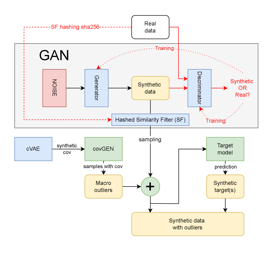
Figure 1: Generalized structure of zGAN. Adapted from the original zGAN paper [7].

The key innovation is the Outliers Conditional Covariance Generator (covGEN) shown in Figure 1, which samples macro outliers from EVT -compatible multivariate families (normal, Laplace, Weibull, Gumbel, Lévy) using covariance matrices derived from real data or from a Conditional VAE (cVAE) [31].

The cVAE supplies covariances by minimizing reconstruction loss and KL divergence; generated outliers are then merged with base GAN samples. For privacy, zGAN applies a hash-based similarity filter [7] to avoid near-duplicates of real records, and for prediction tasks, a classification-style Target Model learns relationships across normal and extreme regions.

In this work, synthetic data refers to zGAN-generated records from typical (non-extreme) regions of the training distribution, while synthetic (macro) outliers are deliberately sampled tail points that mimic shocks. Baselines use only real pre-shock data; stabilized models use a mix of real + synthetic, optionally with a set share of outliers. This distinction matters because stability gains under shocks primarily come from exposure to plausible tails.

As an example of synthetic data and synthetic outliers, Figure 2 shows the distribution plots of the “tjs/usd” column (see Appendix G) from the Tajikistan dataset ($A_{1}$).

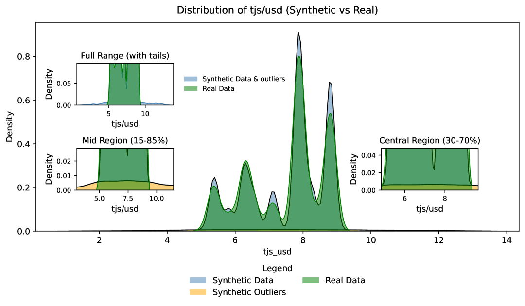
(a) 5% outliers

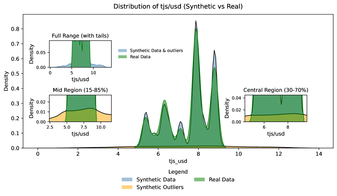
(b) 10% outliers

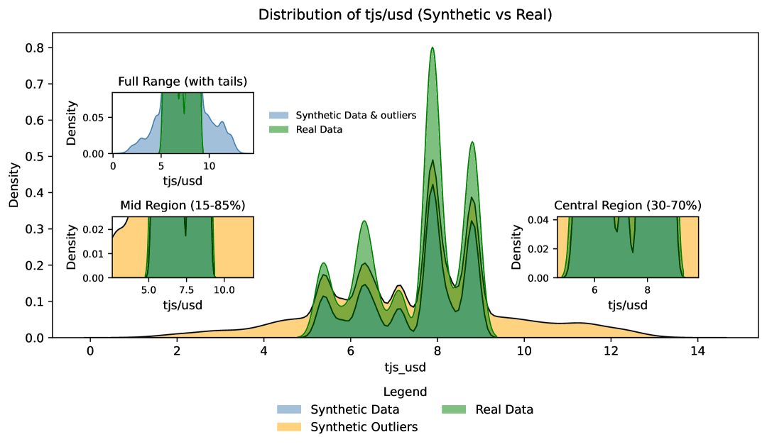
(c) 50% outliers

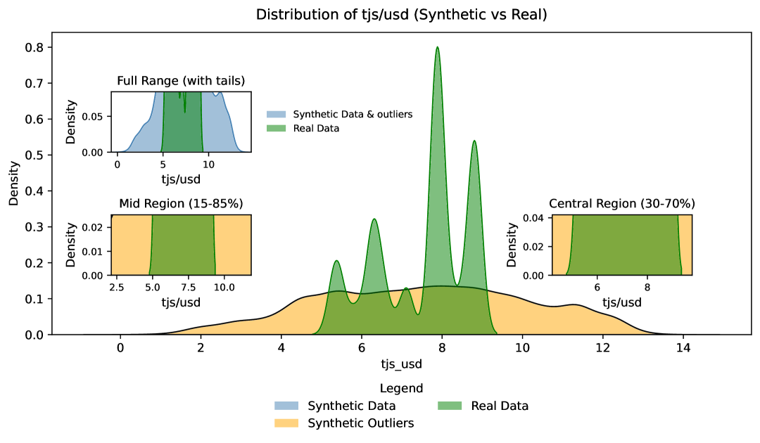
(d) 100% outliers

Figure 2: Distribution plots of real and synthetic data for the “tjs/usd” column from the Tajikistan dataset ($A_{1}$). (a) 5% outliers; (b) 10% outliers; (c) 50% outliers; (d) 100% outliers.

Figure 2 shows the marginal distribution of the “tjs/usd” column from the Tajikistan dataset ($A_{1}$). This column represents a macroeconomic indicator describing the exchange rate of the national currency of the Republic of Tajikistan (somoni) against the U.S. dollar. In each subfigure (a) – (d), the main plot includes zoomed-in insets: in the top-left inset, synthetic data with synthetic outliers are shown in blue, while the overlaid real data distribution is highlighted in green. The other two zoomed-in plots separately display the distribution of outliers, i.e., the tails, and the distribution of the main body of synthetic and real data.

Figure 3 shows the Uniform Manifold Approximation and Projection (UMAP) [32] embeddings of the Tajikistan dataset ($A_{1}$).

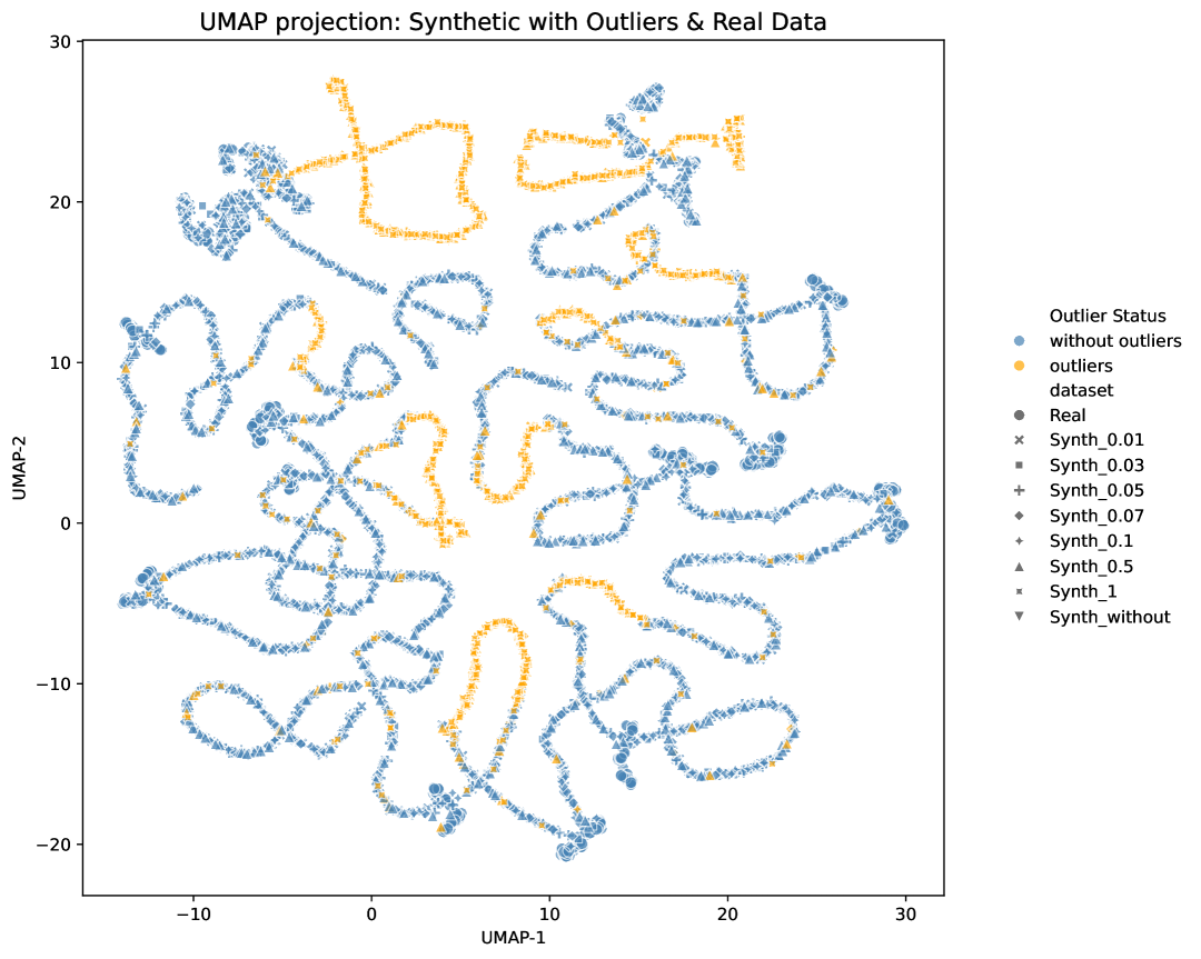
(a)

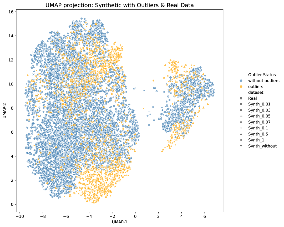
(b)

Figure 3: UMAP projections of the Tajikistan dataset ($A_{1}$).

To construct the embeddings shown in Figure 3 (a) and (b), all generated synthetic datasets, with and without outliers, along with the real dataset, were combined into a single dataset. The merged Tajikistan dataset was then used to obtain the displayed embeddings.

The embedding variant shown in subfigure (a) differs from that in subfigure (b) solely in terms of preprocessing. The key distinction between the two preprocessing approaches lies in the feature composition and scaling: the first variant excludes categorical variables and does not apply normalization to numerical features, which may cause features with larger numeric ranges to dominate the UMAP space; the second variant retains all encoded categorical features and applies standardization to all variables, ensuring that each feature contributes equally to the dimensionality reduction results regardless of its original scale. Although subfigure (b) represents a more appropriate approach for algorithms sensitive to feature scaling, since the embedding is used purely for visual analysis, variant (a) is also applicable and appears more interpretable.

As shown in Figures 2 and 3, the outliers generated by zGAN are, in most cases, visually distinguishable from the synthetic data of the main distribution, while the synthetic data corresponding to the main distribution appear realistic, that is, they are barely distinguishable from the real data distribution. However, some outliers are still formed within the main distribution, which is particularly evident when a large number of outliers are present in the synthetic data, for instance, in the variant with $50\%$ outliers shown in Figure 2 (c).

The inclusion of some outliers within the main distribution is due to the post-processing of outliers performed by the covGEN module, see Figure 1. The post-processing step involves shifting negative outliers toward the center of the distribution, ensuring that the resulting outliers remain plausible within the logical constraints of the features. For example, the exchange rate of somoni to the U.S. dollar cannot take negative values.

Appendix B Experimental Pipeline

The experimental pipeline consists of three main components: data preparation, ML modeling and evaluation, and the computation of the proposed quality metrics that characterize the stability of ML models under model drift conditions.

Figure 4 shows the experimental pipeline in the OOT setting with the identification of the shock portion.

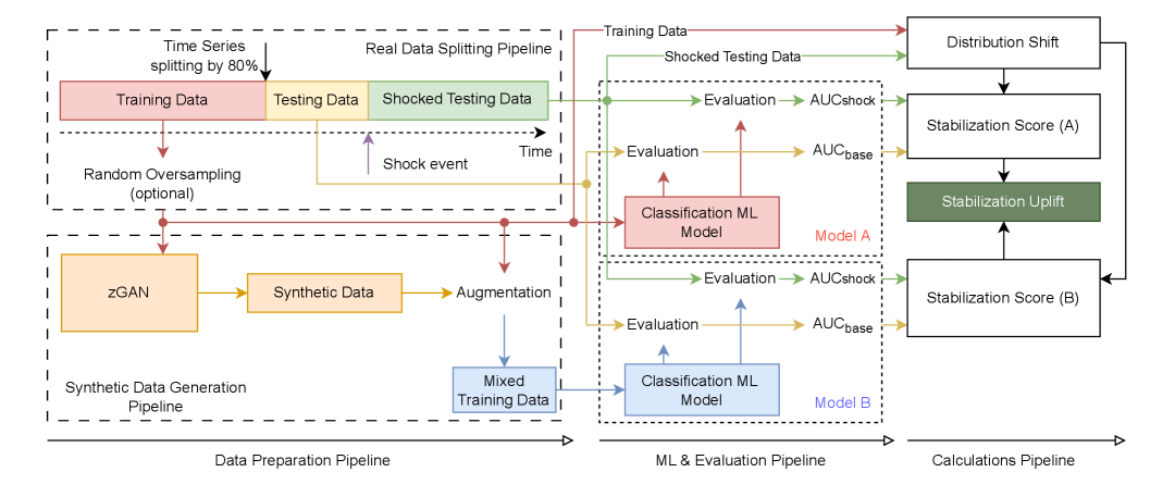
Figure 4: Experimental Pipeline.

The first stage of the experimental pipeline is data splitting, illustrated in the block “Real Data Splitting Schema” in Figure 4. The real data is partitioned according to the OOT principle into pre-shock data (Training and Testing) and post-shock data (Shocked Testing Data). The shock event is defined as the moment after which model drift is expected to occur, with concrete examples provided in Appendix C. The pre-shock data is further divided into training and testing sets in an 80/20 ratio using random sampling.

The resulting real data is used to train the A-model, which is evaluated using the metrics AUC_base, calculating performance in the pre-shock period, and AUC_shock, calculating performance in the shock and post-shock periods.

To construct the B-model, which is assessed for stability against drift, the real training data is optionally upsampled to 10,000 samples through random resampling. These data are then used to train the zGAN model, which generates synthetic samples. The synthetic data is mixed with the original real data at a 50/50 ratio, and the combined dataset is used to train the B-model. The B-model is likewise evaluated using AUC_base and AUC_shock.

To ensure the reliability of the final metrics, a Monte Carlo methodology is applied: each dataset is split into 51 subsets, on each of which a model is trained and evaluated. From the resulting 51 AUC values, the median and range are computed. The experimental methodology follows the approach described in  [7].

Appendix C Shock Origins and Split Configuration

Table 2 summarizes, for each dataset, whether a concrete external shock was identified, the split type, the shock period, and the calculated Distribution Shift (DS).

Table 2: Characteristics of datasets (shock origin, split and macro-financial covariates availability). OOT = Out-of-Time, OOS = Out-of-Sample. ${\color[rgb]{0,1,0}\checkmark}$ is available, ${\color[rgb]{1,0,0}\times}$ is unavailable.

Dataset	Split	Shock Event	Shock Date	Macro-financial covariates	DS
$A_{1}$ (Tajikistan)	OOT	Trade conflict	2018-03-22	${\color[rgb]{0,1,0}\checkmark}$	0.2250
$A_{4}$ (Uzbekistan)	OOS	${\color[rgb]{1,0,0}\times}$	${\color[rgb]{1,0,0}\times}$	${\color[rgb]{0,1,0}\checkmark}$	0.0050
$A_{5}$ (Kazakhstan)	OOT	Armed conflict	2021-12-30	${\color[rgb]{1,0,0}\times}$	0.1212
$A_{6}$ (Jordan)	OOS	${\color[rgb]{1,0,0}\times}$	${\color[rgb]{1,0,0}\times}$	${\color[rgb]{1,0,0}\times}$	0.0026
$A_{9}$ (Azerbaijan)	OOT	Armed conflict	2021-12-30	${\color[rgb]{0,1,0}\checkmark}$	0.1802
Open Data (LC)	OOT	Trade conflict	2018-03-22	${\color[rgb]{0,1,0}\checkmark}$	0.1193

It is important to note that the lowest Distribution Shift is observed when data is split using the OOS principle, as shown in Table 2. This indicates a low level of model drift, which is expected for data that is not affected by shock events.

Appendix D Algorithmic Description

To compute the Distribution Shift (1), we used tools from the SDV library designed for working with tabular data. The Metadata  method was used to automatically identify categorical and numerical column names, while the TVComplement  and KSComplement  methods were used to calculate $d_{TV}(c)$ and $d_{KS}(n)$, respectively. The pseudocode of the DS algorithm is shown in structure 1.

Algorithm 1 Computation of Distribution Shift

1:Base dataset $D_{\text{base}}$, Shock dataset $D_{\text{shock}}$

2:$M\leftarrow\texttt{detect metadata}(D_{\text{base}})$

3:$C\leftarrow$ categorical columns from $M$

4:$N\leftarrow$ numerical columns from $M$

5:$S\leftarrow[\ ]$ $\triangleright$ List of shift values

6:for all $c\in C$ do

7:  $s\leftarrow 1-\texttt{TVComplement}(D_{\text{base}}[c],D_{\text{shock}}[c])$

8:  Append $s$ to $S$

9:end for

10:for all $n\in N$ do

11:  $s\leftarrow 1-\texttt{KSComplement}(D_{\text{base}}[n],D_{\text{shock}}[n])$

12:  Append $s$ to $S$

13:end for

14:if $S$ is not empty then

15:  return $\texttt{mean}(S)$

16:else

17:  return $0.0$

18:end if

It is worth noting that the pseudocode in Algorithm 1 uses 1-TVComplement and similarly for KSComplement, since the metric implementations in the library are designed such that higher scores indicate better quality.

The pseudocode of the SS implementation (2) is shown in structure 2.

Algorithm 2 Computation of Stabilization Score

1:Base AUC $\hat{A}_{\text{base}}$, Shock AUC $\hat{A}_{\text{shock}}$, Distribution Shift $d$

2:Stabilization Score $s$

3:if $\hat{A}_{\text{base}}<0.5$ then

4:  $\hat{A}_{\text{base}}\leftarrow 1-\hat{A}_{\text{base}}$

5:end if

6:if $\hat{A}_{\text{shock}}<0.5$ then

7:  $\hat{A}_{\text{shock}}\leftarrow 1-\hat{A}_{\text{shock}}$

8:end if

9:$\varepsilon\leftarrow 10^{-5}$

10:$\Delta A\leftarrow|\hat{A}_{\text{base}}-\hat{A}_{\text{shock}}|$

11:$v\leftarrow 1+\log(1+d+\varepsilon)$

12:$s\leftarrow 1-\frac{\Delta A}{v}$

13:return $s$

The transformation $AUC<0.5\rightarrow 1-AUC$ in Algorithm 2 is necessary to invert the model, allowing models with, for example, flipped labels to be treated as informative. This approach ensures that the SS remains within an intuitively interpretable range of values, from 0.5 to 1. For example, in cases with label noise or label permutation, one of the AUC values may approach zero while the other remains close to one. Under such conditions, SS could otherwise be incorrectly spread across the full range from 0 to 1.

The final Stabilization Uplift score (3) is computed according to the algorithm presented in Algorithm 3.

Algorithm 3 Computation of Stabilization Uplift

1:AUC values for model A: $\hat{A}_{\text{base}}^{A},\hat{A}_{\text{shock}}^{A}$; model B: $\hat{A}_{\text{base}}^{B},\hat{A}_{\text{shock}}^{B}$; Distribution Shift $d$

2:Stabilization Uplift score $SU$

3:$k_{1}\leftarrow 100$   $k_{2}\leftarrow 1000$   $k_{3}\leftarrow 1000$

4:for $x\in\{\hat{A}_{\text{base}}^{A},\hat{A}_{\text{shock}}^{A},\hat{A}_{\text{base}}^{B},\hat{A}_{\text{shock}}^{B}\}$ do

5:  if $x<0.5$ then

6:   $x\leftarrow 1-x$

7:  end if

8:end for

9:$w_{A}\leftarrow 1-\dfrac{1}{1+\exp\!\big(k_{1}(\hat{A}_{\text{shock}}^{A}-\hat{A}_{\text{base}}^{A})\big)}$ $\triangleright$ Stability weights

10:$w_{B}\leftarrow 1-\dfrac{1}{1+\exp\!\big(k_{1}(\hat{A}_{\text{shock}}^{B}-\hat{A}_{\text{base}}^{B})\big)}$

11:$w\leftarrow 1-\dfrac{1}{1+\exp\!\big(k_{2}(\hat{A}_{\text{shock}}^{B}-\hat{A}_{\text{shock}}^{A})\big)}$ $\triangleright$ Relative superiority on shocked data

12:$w_{\text{sup}}\leftarrow 1-\dfrac{1}{1+\exp\!\big(k_{3}\big[(\hat{A}_{\text{base}}^{B}-\hat{A}_{\text{base}}^{A})+(\hat{A}_{\text{shock}}^{B}-\hat{A}_{\text{shock}}^{A})\big]\big)}$ $\triangleright$ Combined superiority

13:$w_{B}^{\prime}\leftarrow w_{B}\cdot w_{\text{sup}}$ $\triangleright$ Adjusted stability weights

14:$w_{A}^{\prime}\leftarrow w_{A}\cdot(1-w_{\text{sup}})$

15:$SS_{A}\leftarrow\text{StabilizationScore}(\hat{A}_{\text{base}}^{A},\hat{A}_{\text{shock}}^{A},d)$ $\triangleright$ Compute SS

16:$SS_{B}\leftarrow\text{StabilizationScore}(\hat{A}_{\text{base}}^{B},\hat{A}_{\text{shock}}^{B},d)$

17:$SU\leftarrow w\cdot(w_{B}^{\prime}\cdot SS_{B}-w_{A}^{\prime}\cdot SS_{A})$ $\triangleright$ Final uplift

18:return $SU$

As shown in Algorithm 3, the final Stabilization Uplift score reflects the stability and quality of model B compared to the baseline model A under a distributional shift. Smooth logistic weights are used to quantify the degradation of model performance between the base and shock scenarios. These weights capture not only the individual stability of each model but also the relative advantage of model B over model A. An additional supervisory weight $w_{\text{sup}}$ further amplifies the contribution of the more stable model. The final score is computed as a weighted difference between the stabilization scores of the two models, accounting for both performance dynamics and distributional change structure.

The problem of selecting the coefficients $k_{1},k_{2},$ and $k_{3}$ is discussed in Appendix F.

The resulting algorithmic framework is used to compute the metrics in a classification task; the description and results of the conducted experiments are presented in the following chapter.

Appendix E Experimental Results

Stabilization Uplift Across Baselines and Outlier Levels

Tables 3–6 report the experimental results for datasets that include macro-variables, for which synthetic outliers were generated accordingly. Table 7 summarizes the results for datasets without macro-variables, where stabilization experiments with synthetic outliers were not conducted, and only experiments with synthetic data without outliers were performed.

Table 3: Stabilization Uplift scores across different outlier levels for Tajikistan dataset ($A_{1}$). Green indicates the highest value, Blue the second highest, and Red the third highest.

Outliers, %	CatBoost	TabPFN	FT-Transformer	HGBoosting	NGBoost	XGBoost	LightGBM	TabNet
without	0.2667	0.8093	0.0000	0.6363	0.0916	0.0000	0.0000	0.8441
1	0.0572	0.6319	0.0000	0.7106	0.1128	0.0000	0.0000	0.6258
3	0.0000	0.5281	0.0000	0.5442	0.1380	0.0000	0.0000	0.2737
5	0.0000	0.2542	0.0000	0.6764	0.0349	0.0000	0.0000	0.3266
7	0.0000	0.6951	0.0000	0.6079	0.1830	0.0000	0.0000	0.6171
10	0.0534	0.6703	0.0000	0.7266	0.5459	0.2362	0.1237	0.0000
50	0.0000	0.4705	0.0000	0.4760	0.0000	0.0000	0.0000	0.7257
100	0.0105	0.8126	0.0000	0.6905	0.4744	0.0000	0.0000	0.4562

Table 4: Stabilization Uplift scores across different outlier levels for Uzbekistan dataset ($A_{4}$). Green indicates the highest value, Blue the second highest, and Red the third highest.

Outliers, %	CatBoost	TabPFN	FT-Transformer	HGBoosting	NGBoost	XGBoost	LightGBM	TabNet
without	0.2667	0.4103	0.0109	0.0000	0.0000	0.0000	0.0000	0.0002
1	0.0000	0.3061	0.0246	0.0000	0.0000	0.0000	0.0000	0.0000
3	0.0000	0.4888	0.0266	0.0000	0.0000	0.0000	0.0000	0.0000
5	0.0086	0.0000	0.0000	0.0000	0.0000	0.0000	0.0000	0.0000
7	0.0000	0.3259	0.0258	0.0000	0.0000	0.0000	0.0000	0.0000
10	0.0000	0.0000	0.0000	0.0000	0.0000	0.0000	0.0000	0.0000
50	0.0000	0.7449	0.0220	0.0000	0.0000	0.0000	0.0000	0.0000
100	0.0000	0.4795	0.0000	0.0000	0.0000	0.0000	0.0000	0.0087

Table 5: Stabilization Uplift scores across different outlier levels for Azerbaijan dataset ($A_{9}$). Green indicates the highest value, Blue the second highest, and Red the third highest.

Outliers, %	CatBoost	TabPFN	FT-Transformer	HGBoosting	NGBoost	XGBoost	LightGBM	TabNet
without	0.1874	0.9827	0.9406	0.0000	0.0001	0.1859	0.6697	0.0000
1	0.6018	0.9863	0.9470	0.0000	0.0058	0.044	0.4001	0.0000
3	0.0150	0.9818	0.3784	0.5642	0.0207	0.0653	0.2549	0.0000
5	0.1272	0.9981	0.9163	0.0000	0.0015	0.1325	0.6295	0.0000
7	0.0786	0.9952	0.9460	0.0000	0.0032	0.3271	0.9196	0.0000
10	0.0037	0.9962	0.9555	0.7394	0.0164	0.1681	0.7486	0.0000
50	0.3238	0.9928	0.9447	0.0000	0.0000	0.0408	0.3750	0.9139
100	0.7496	0.9906	0.9540	0.1365	0.0143	0.1601	0.6879	0.0000

Table 6: Stabilization Uplift scores across different outlier levels for Open dataset. Green indicates the highest value, Blue the second highest, and Red the third highest.

Outliers, %	CatBoost	TabPFN	FT-Transformer	HGBoosting	NGBoost	XGBoost	LightGBM	TabNet
without	0.0000	0.0000	0.6971	0.0000	0.0000	0.0000	0.0000	0.0131
1	0.1680	0.0583	0.8861	0.0000	0.0000	0.0000	0.0000	0.0000
3	0.0578	0.0000	0.6198	0.0000	0.0000	0.0000	0.0000	0.2880
5	0.0000	0.0000	0.1671	0.0000	0.0000	0.0000	0.0000	0.0000
7	0.0000	0.0000	0.7289	0.0000	0.0000	0.0000	0.0000	0.4809
10	0.0000	0.0000	0.7896	0.0000	0.0000	0.0000	0.0000	0.1820
50	0.0000	0.0000	0.0000	0.0000	0.0000	0.0000	0.0000	0.0010
100	0.0000	0.0000	0.8884	0.0000	0.0000	0.0000	0.0000	0.6237

Table 7: Stabilization Uplift scores across different datasets without outliers

Datasets	CatBoost	TabPFN	FT-Transformer	HGBoosting	NGBoost	XGBoost	LightGBM	TabNet
Kazakhstan ($A_{5}$)	0.3526	0.8343	0.4758	0.0000	0.0000	0.0220	0.0164	0.0002
Jordan ($A_{6}$)	0.0251	0.0000	0.0544	0.5704	0.2881	0.0000	0.0000	0.3496

Across model–dataset pairs, adding a non-zero share of synthetic outliers improves stability in 135 out of 256 cases, corresponding to approximately $53\%$, as shown in Tables 3–6.

For HGBoosting, NGBoost, XGBoost, and LightGBM, stabilization uplift is achieved in $50\%$ of cases, i.e., for 2 out of 4 datasets with macro-variables, when an additional share of synthetic outliers is introduced. For FT-Transformer, stabilization uplift is observed in $75\%$ of cases, and for CatBoost, TabPFN, and TabNet it is observed in $100\%$ of cases.

Across model–dataset pairs, adding a non-zero share of synthetic outliers improves stability in the vast majority of cases. Notable patterns are:

1. flexible architectures (TabPFN, FT-Transformer) benefit most;

2. the optimal outlier share is non-monotonic and typically small (5–10%);

3. gains correlate with DS magnitude (largest for $A_{1}$/$A_{9}$, attenuated for low-DS $A_{4}$/$A_{6}$).

While a few best single configurations occur without outliers (e.g., TabNet on $A_{1}$), counting across all baselines shows more models improve with outliers than without, aligning with our conclusion that deliberate tail exposure enhances post-shock stability.

The Stabilization Uplift (3) metric takes a zero or near-zero value when stabilization methods fail to improve stability, i.e., when model B exhibits a larger difference between $\hat{A}_{\text{base}}$ and $\hat{A}_{\text{shock}}$ compared to model A. If the applied stabilization method leads to a decrease in $\hat{A}_{\text{shock}}^{B}$ relative to $\hat{A}_{\text{shock}}^{A}$; that is, if the model’s performance after stabilization deteriorates compared to the non-stabilized model, then Stabilization Uplift decreases logistically according to the sigmoid steepness parameter $k_{2}$, as shown in Algorithm 3. This approach to stability computation reflects the principle that the value of stability gains diminishes when model quality degrades as a result of applying stabilization methods.

This formulation also explains why the outcomes vary across the four datasets. On datasets with pronounced shocks and higher feature variability, models tend to stabilize when synthetic outliers are introduced, whereas on datasets with weaker shifts or more rigid feature structures, stabilization effects may be negligible or even detrimental. At the same time, architectural flexibility plays a critical role: highly expressive models (e.g., TabPFN, FT-Transformer) can adapt to tail augmentation and convert outliers into useful signal, while tree-based ensembles or boosting methods may fail to leverage the additional variability. Consequently, some models exhibit consistent stability gains, while others remain unaffected or even degrade, illustrating the joint influence of dataset characteristics and model architecture on stabilization outcomes.

Stabilization Uplift and AUC Components

For the open dataset available in the project’s GitHub repository, complete tables with all intermediate results and metrics are provided. The reported AUC values can be used to demonstrate how they relate to the final Stabilization Uplift metric, helping to better understand the behavior of this metric.

In Figure 5, radial plots illustrate the values of AUC and Stabilization Uplift for each baseline model and for different proportions of outliers in the synthetic data.

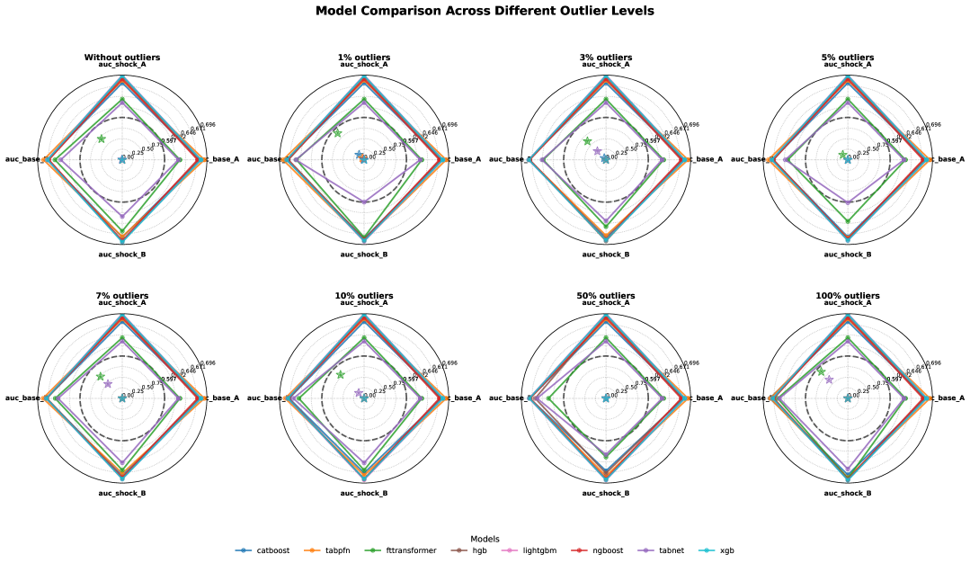
Figure 5: Radial plots of AUC and Stabilization Uplift for the Open Dataset, for each outlier percentage.

In Figure 5, each radial plot is constructed for the AUC and SU metric values corresponding to a specific proportion of outliers in the synthetic data, with different colors representing individual baselines. On the outer ring, points connected by lines indicate the AUC values, while on the inner ring, asterisks mark the SU metric values.

The plots reveal a competition in SU values between the FT-Transformer and TabNet models, with the former generally outperforming the latter. Examining the AUC values, for instance at $7\%$ outliers, shows that the AUCs are largely comparable. However, the FT-Transformer exhibits a slight increase in $\hat{A}_{\text{base}}^{B}$ relative to TabNet, along with a somewhat larger increase in $\hat{A}_{\text{shock}}^{B}$, such that for both models $\hat{A}_{\text{shock}}^{B}>\hat{A}_{\text{base}}^{B}$. This AUC configuration represents a scenario where synthetic data stabilized the model, leading to a performance gain, while the pre-shock model shows a slightly smaller improvement compared to the post-shock AUC. In this case, each model receives an SU value roughly proportional to the AUC gain of model B relative to model A and the difference between post-shock and pre-shock AUC.

In the second case, at $10\%$ outliers, TabNet exhibits a larger pre-shock AUC gain relative to post-shock, meaning that the quality improvement from synthetic data with outliers primarily benefited the model less affected by the shock. Here, SU penalizes the model, resulting in a lower SU compared to FT-Transformer, since the synthetic outlier data substantially prepared the latter for the shock.

To observe the behavior of the SU metric in relation to AUC at different outlier percentages in the synthetic data, radial plots were constructed for each ML model, as shown in Figure 6. These plots exclude zero Stabilization Uplift values.

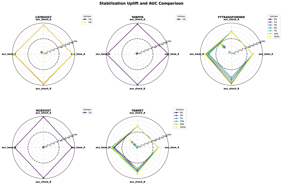
Figure 6: Radial plots of AUC and Stabilization Uplift for the Open Dataset, for each ML-model.

A visual analysis of Figure 6 reveals the underlying logic of the Stabilization Uplift metric. Specifically, higher SU values are assigned when an ML model achieves superior performance on the post-shock test depending on the outlier proportion, given an overall advantage of model B over model A. This takes into account the distance between the models’ Stabilization Scores (2), as illustrated, for example, by FT-Transformer and TabNet.

Appendix F On the Selection of Optimal and Quasi-Optimal Coefficients

The selection of optimal coefficients for formula (3) may involve several conditions important for the interpretability, fairness, and optimizability of the metric (in the case of its use as a loss function).

The interpretability of the metric can be verified using expert evaluations. For such a case, a table of expert assessments should be constructed, consisting of the shock and baseline AUC values for models A and B, as well as the DS (1) values, and the expert evaluations of SU themselves. In the general case, the problem can be described by the following expression:

$$\min_{\boldsymbol{\theta}\in\mathcal{K}}\;\mathcal{J}(\boldsymbol{\theta})\;=\;\frac{1}{N}\cdot\sum_{i=1}^{N}c^{(i)}\,\cdot\ell\!\left(\widehat{\mathrm{SU}}^{(i)}(\boldsymbol{\theta})-s^{(i)}\right)\;+\;\lambda\,\cdot\mathcal{R}(\boldsymbol{\theta}),$$ (4)

where $\boldsymbol{\theta}=(k_{1},k_{2},k_{3})$ are the coefficients; $N$ — the number of data points (e.g., DS values or input–output pairs for SU); $c^{(i)}$ is the confidence weight reflecting the reliability or importance of the i-th expert assessment; $\ell(u)$ is a loss function (e.g., $\ell(u)=u^{2}$ or Huber), $u^{(i)}=\widehat{\mathrm{SU}}^{(i)}(\boldsymbol{\theta})-s^{(i)}$; $\mathcal{R}(\boldsymbol{\theta})$ is a regularizer (e.g., $\mathcal{R}(\boldsymbol{\theta})=\|\boldsymbol{\theta}\|_{2}^{2}$), and $\lambda\geq 0$.

The expert-aligned, interpretable coefficients are then defined by:

$$\boldsymbol{\theta}^{\star}=\arg\min_{\boldsymbol{\theta}\in\mathcal{K}}\mathcal{J}(\boldsymbol{\theta}),$$ (5)

with $\widehat{\mathrm{SU}}^{(i)}(\boldsymbol{\theta})$ computed per (2)–(3) using the $i$-th row of the expert table.

The fairness of the SU metric can be considered with respect to the DS metric. It is important that, for the chosen coefficients, the SU metric preserves its logarithmic growth with respect to changes in DS. The original objective function $\mathcal{J(\boldsymbol{\theta})}$ (4) is extended by incorporating expert annotations and introducing a reference logarithmic form $a\log(b\,\mathrm{DS}+c)$ as part of the regularization, resulting in the following problem formulation:

$$\min_{\boldsymbol{\theta}\in\mathcal{K},\;a>0,\;b>0,\;c\in\mathbb{R}}\;\mathcal{J}(\boldsymbol{\theta})\;=\;\frac{1}{N}\sum_{i=1}^{N}c^{(i)}\cdot\ell\!\left(\widehat{\mathrm{SU}}^{(i)}(\boldsymbol{\theta})-s^{(i)}\right)\;+\;\mathcal{R}(\boldsymbol{\theta},a,b,c),$$ (6)

where $\boldsymbol{\theta}$ is the vector of model parameters to be optimized, $\mathcal{K}$ is the feasible set of parameters defined by hard constraints (monotonicity, concavity, slope bound, etc.); $\mathcal{R}(\boldsymbol{\theta},a,b,c)$ — the combined regularization term: $\lambda_{\log}\,\mathcal{P}_{\log}$ — penalty for deviation from the reference logarithmic form $a\log(b\,\mathrm{DS}+c)$; $\lambda_{\mathrm{TV}}\,\mathcal{P}_{\mathrm{TV}}$ — total variation smoothing to suppress abrupt jumps; $\lambda_{\mathrm{curv}}\,\mathcal{P}_{\mathrm{curv}}$ — curvature penalty to reduce local bends in the curve.

Under the constraints of SU matching expert assessments and preserving the logarithmic form (6), stability of ML models can also be considered, which corresponds to the second fairness task, formulated as follows:

$$\min_{\boldsymbol{\theta}\in\mathcal{K},\;a>0,\;b>0,\;c\in\mathbb{R}}\;\mathcal{J}(\boldsymbol{\theta})\;=\;\frac{1}{N}\sum_{i=1}^{N}c^{(i)}\cdot\ell\!\left(\widehat{\mathrm{SU}}^{(i)}(\boldsymbol{\theta})-s^{(i)}\right)\;+\;\mathcal{R}(\boldsymbol{\theta},a,b,c,\epsilon),$$ (7)

where $\boldsymbol{\theta}$ is the vector of model parameters to optimize, $\mathcal{K}$ is the feasible set defined by hard constraints (monotonicity, concavity, slope bound, etc.), $a,b,c$ are the parameters of the reference logarithmic form $a\log(b\,\mathrm{DS}+c)$, and $\mathcal{R}(\boldsymbol{\theta},a,b,c,\epsilon)$ is the combined regularization term: $\lambda_{\log}\,\mathcal{P}_{\log}$ — penalty for deviation from the reference log-form, $\lambda_{\mathrm{TV}}\,\mathcal{P}_{\mathrm{TV}}$ — total variation smoothing to suppress abrupt jumps, $\lambda_{\mathrm{curv}}\,\mathcal{P}_{\mathrm{curv}}$ — curvature penalty to reduce local bends, $\lambda_{\epsilon}\,\mathcal{P}_{\epsilon\text{-robust}}$ — stability penalty ensuring SU remains stable within an $\epsilon$-range of variations of model AUC, i.e.,

$$\mathcal{P}_{\epsilon\text{-robust}}(\boldsymbol{\theta})=\sum_{i=1}^{N}\max_{\text{AUC}^{(i)}\in[\text{AUC}^{(i)}_{0}-\epsilon,\text{AUC}^{(i)}_{0}+\epsilon]}\left|\widehat{\mathrm{SU}}^{(i)}(\boldsymbol{\theta},\text{AUC}^{(i)})-\widehat{\mathrm{SU}}^{(i)}(\boldsymbol{\theta},\text{AUC}^{(i)}_{0})\right|.$$

The search for the coefficients in these cases (6), (7) is formulated analogously to (5).

If the Stabilization Uplift (SU) is used as a loss function, its theoretical optimizability can be established under standard assumptions. Let the parameter vector $\boldsymbol{\theta}=(k_{1},k_{2},k_{3})$ be restricted to the compact set

$$\mathcal{K}=\{(k_{1},k_{2},k_{3}):0\leq k_{i}\leq K_{i},\;i=1,2,3\},$$

where $K_{i}>0$ are expert-chosen upper bounds ensuring positive and bounded coefficients, which in turn guarantee monotone and interpretable responses of the SU to variations in AUC. Let the total objective function be

$$\mathcal{J}_{\text{total}}(\boldsymbol{\theta})=\mathcal{J}(\boldsymbol{\theta})+\mathcal{R}(\boldsymbol{\theta},a,b,c,\epsilon),$$

where $\mathcal{J}$ calculates the discrepancy between predicted and target SU values, and $\mathcal{R}$ is a continuous regularization term including penalties for deviation from the reference logarithmic form, total variation, curvature, and stability with respect to $\epsilon$-level variations in model AUC. Under the assumption that $\mathcal{J}_{\text{total}}$ is continuous on the compact set $\mathcal{K}$, the Weierstrass extreme value theorem ensures the existence of at least one optimal parameter vector $\boldsymbol{\theta}^{*}\in\mathcal{K}$ that minimizes $\mathcal{J}_{\text{total}}$. Therefore, by enforcing compactness of the parameter set and continuity of the objective and regularization terms, the SU is theoretically well-defined as a loss function and the corresponding optimization problem is guaranteed to be solvable in principle.

The search for optimal coefficients assumes the availability of a complete set of expert evaluations, AUC variants, and DS metric values. In practice, this is difficult to achieve; therefore, in real-world tasks, it is possible to search for quasi-optimal coefficients by having experts specify, for example, three SU points equal to 0, 0.5, and 1, followed by performing optimization computations. In this work 3, the selection of coefficient values was carried out using a quasi-optimal approach.

The coefficients obtained as a result of the quasi-optimal search are presented in Table 8.

Table 8: Logistic slope hyperparameters for Stabilization Uplift used in all experiments.

Scope	$k_{1}$	$k_{2}$	$k_{3}$
All datasets / all models (default)	100	1000	1000

A single global set of $(k_{1},k_{2},k_{3})$ was used for all datasets and models, without per-dataset tuning. The values were determined once using the quasi-optimal procedure described above under monotonicity and concavity constraints, and are presented in Table 8. A coarse sensitivity sweep with $k_{1}\in{50,100,200}$, $k_{2}\in{500,1000,2000}$, and $k_{3}\in{500,1000,2000}$ confirmed that all qualitative conclusions remain unchanged. Reported scores correspond to the median values over 51 Monte Carlo splits.

Appendix G Specialized Datasets for Developing Economies

We provide additional details regarding our private datasets.

Table 9: Description of Tajikistan dataset ($A_{1}$) columns

Feature	Dtype	Description
age	int64	Age of the client
gender	int64	Gender of the client
amount_smn	float64	Loan amount
duration	float64	Duration of loan
int_rate	float64	Interest rate
credit_history_count	int64	Number of loans previously taken loans
dependants	float64	Number of dependants in family
mon_remit	float64	Monthly remittance (Macro variable)
mon_payment	float64	Monthly payment
int_amount	float64	Calculated interest amount
usd_rate	float64	USD/Somoni rate (Macro variable)
alum_price	float64	Aluminium price (Macro variable)
oil_price	float64	Oil price (Macro variable)
cotton_price	float64	Cotton price (Macro variable)
tjs_usd	float64	Somoni/USD rate (Macro variable)
is_bad60	int64	Target variable (Bad/Good loan)

Table 10: Statistical characteristics of the Tajikistan dataset ($A_{1}$) for numerical variables

Feature	Dtype	Missing	Unique	Mean	Std	Skewness	Kurtosis	Min	25%	Median	75%	Max	IQR
age	int64	0	63	41.5845	11.8583	0.2574	-0.8968	18	32	41	51	80	19
gender	int64	0	2	0.6250	0.4841	-0.5162	-1.7335	0	0	1	1	1	1
amount_smn	float64	0	1699	5249.441	3897.815	1.7069	4.2671	23.6	2500	4000	7000	30000	4500
duration	float64	0	67	14.0019	4.4964	2.2536	19.0871	1	12	12	18	120	6
int_rate	float64	0	39	0.3619	0.0410	-1.1243	4.1508	0	0.34	0.36	0.40	0.47	0.06
credit_history_count	int64	0	84	2.5480	2.7751	7.7530	127.332	1	1	2	3	84	2
dependants	float64	0	18	5.2107	1.9663	1.1464	3.0468	0	4	5	6	17	2
mon_remit	float64	0	26	1.94e+08	5.23e+07	-0.0198	-0.9197	9.50e+07	1.65e+08	1.81e+08	2.20e+08	2.77e+08	5.51e+07
mon_payment	float64	0	12648	471.9793	375.2203	5.7272	120.661	4.6	249.91	379.09	577.58	15525	327.67
int_amount	float64	0	12548	1359.216	1292.326	2.4415	10.2900	0	513.92	967.96	1729.66	29815.2	1215.74
usd_rate	float64	0	71	7.7318	1.0970	-0.5810	-0.9108	5.5209	6.6207	7.8759	8.8050	11.405	2.1843
alum_price	float64	0	77	1815.195	238.2081	0.3474	-0.9940	1459.93	1592.36	1804.04	2030.01	2446.65	437.65
oil_price	float64	0	77	51.4332	9.5819	0.0242	-0.0631	21.04	45.69	50.90	57.54	76.73	11.85
cotton_price	float64	0	75	78.2416	8.3149	0.2463	-1.1698	63.53	70.28	78.92	85.16	97.71	14.88
tjs_usd	float64	0	67	7.6490	1.1358	-0.6587	-0.7294	5.3074	6.6207	7.8719	8.8038	11.32	2.1831
is_bad60	int64	0	2	0.0664	0.2490	3.4824	10.1273	0	0	0	0	1	0

Table 11: Statistical characteristics of the Tajikistan dataset ($A_{1}$) for categorical variables

Feature	Dtype	Missing	Unique	Freq	Percent Top
sector	object	0	6	142172	40.97%
education	object	0	5	206582	59.53%
marital_status	object	0	5	278051	80.12%
district	object	0	36	46681	13.45%

Table 12: Description of the Uzbekistan dataset ($A_{4}$) columns

Feature	Dtype	Description
gender	int64	Client’s gender
monthly_payment	float64	Loan monthly payment
contract_amount	float64	Previous loan contract amount
item_amount	float64	Amount of loan items
age	int64	Client’s age
ltv	float64	Loan to value ratio
contract_duration	int64	Duration of loan
Interest Rate	int64	Yearly interest rate
Balance of Trade	float64	Balance of trade (macro variable)
Inflation Rate	float64	Inflation rate (macro variable)
Current Account	float64	Current client’s loans
Remittances	float64	Remittances (macro variable)
usd_uzs	float64	USD/UZS rate
rub_uzs	float64	RUB/UZS rate
target	int64	Target variable

Table 13: Statistical characteristics of the Uzbekistan dataset ($A_{4}$) for numerical variables

Feature	Dtype	Missing	Unique	Mean	Std	Skewness	Kurtosis	Min	25%	Median	75%	Max	IQR
gender	int64	0	2	0.6001	0.4899	-0.4087	-1.8330	0	0	1	1	1	1
monthly_payment	float64	0	12144	425133.4	263025.7	1.9526	5.4135	83333	255267	354000	522100	2577855	266833
contract_amount	float64	0	12183	5032402	3098996	1.9644	5.5727	1000000	3036000	4195200	6182400	30934265	3146400
item_amount	float64	0	5508	3747260	19730909	179.4820	32655.73	100000	2142000	3240000	4609000	3.59e+09	2467000
age	int64	0	57	36.6165	9.4628	0.5756	-0.3888	19	29	35	43	75	14
ltv	float64	0	11665	2.3912	5.6335	9.8632	138.227	0.0015	1	1	1.5194	156.0924	0.5194
contract_duration	int64	0	4	11.8973	0.7849	-8.3539	73.5403	3	12	12	12	12	0
Interest Rate	int64	0	4	14.9967	1.2978	0.7503	-1.2519	14	14	14	17	17	3
Balance of Trade	float64	0	17	-873.39	648.5264	1.3614	1.3750	-1826.6	-1172.8	-1072	-798	763.2	374.8
Inflation Rate	float64	0	12	10.9321	0.6566	1.0281	0.1271	10	10.5	10.8	11.1	12.3	0.6
Current Account	float64	5989	5	-1351.52	468.5964	1.4784	4.7791	-1869.2	-1869.2	-1203.63	-1203.63	453.07	665.57
Remittances	float64	5989	5	2062.969	615.3457	2.7211	10.2272	1403.43	1884.28	1884.28	2390.8	4801.91	506.52
usd_uzs	float64	0	413	10867.16	266.6989	0.9254	-0.3744	10527.73	10666.01	10752.86	11030.51	11539.65	364.49
rub_uzs	float64	0	412	149.4125	21.6284	-0.6057	2.1259	76.3182	144.2943	146.5607	154.0946	206.7358	9.80
target	int64	0	2	0.0777	0.2676	3.1561	7.9607	0	0	0	0	1	0

Table 14: Statistical characteristics of the Uzbekistan dataset ($A_{4}$) for categorical variables

Feature	Dtype	Missing	Unique	Freq	Percent Top
category	object	0	20	12273	36.56%
region	object	0	12	13266	39.52%
partner_id_top30	object	0	31	7981	23.77%
partner_filtered_15	object	0	16	20027	59.66%

Table 15: Description of the Kazakhstan dataset ($A_{5}$) columns

Feature	Dtype	Missing	Description
flag_fin	int64	0
BAD	float64	0	Target variable
credit_amount	float64	0	Loan amount
LOAN_AMOUNT	float64	0	Loan amount
DURATION	float64	0	Loan duration
Gender	float64	0	Client’s gender
AGE	int64	0	Client’s age
credit_history_count	float64	16270	Credit history count
OCCUPATION	float64	4769	Client’s occupation
NUMBEROFCHILDREN	float64	254141	Number of client’s children
BUDGETTOTALINCOME	float64	19	Total income budget
GCVPSAL	float64	15635
hasCar	float64	4818	Has client a car
has_house	float64	16392	Has client a house
cumulative_dpd	float64	16511	Cumulative due date
max_dpd	float64	16511	Maximum due date
MOBILEPHONE	float64	3	Has client a mobile phone
repeated_client	int64	0	Is client a repeated client

Table 16: Statistical characteristics of the Kazakhstan dataset ($A_{5}$) for numerical variables

Feature	Dtype	Missing	Unique	Mean	Std	Skewness	Kurtosis	Min	25%	Median	75%	Max	IQR
flag_fin	int64	0	1	1.0000	0.0000			1	1	1	1	1	0
BAD	float64	0	2	0.0249	0.1558	6.1003	35.2139	0	0	0	0	1	0
credit_amount	float64	0	87821	205889.9	170044.5	2.0781	6.4357	7495	89990	151980	262000	2000000	172010
LOAN_AMOUNT	float64	0	115643	211923.9	172667.9	2.0275	6.0728	7495	94092	158125	270827	2000000	176735
DURATION	float64	0	36	17.0035	13.1665	1.1281	0.3989	3	6	12	24	60	18
Gender	float64	0	2	1.5861	0.4925	-0.3496	-1.8778	1	1	2	2	2	1
AGE	int64	0	57	41.6174	12.7692	0.4234	-0.7103	18	31	40	51	74	20
credit_history_count	float64	16270	242	12.7823	38.1648	14.8352	442.1289	1	4	7	12	3000	8
OCCUPATION	float64	4769	28	15.1335	6.8169	1.0544	0.0771	1	12	13	19	31	7
NUMBEROFCHILDREN	float64	254141	12	0.4259	0.8538	2.5050	8.2227	0	0	0	1	15	1
BUDGETTOTALINCOME	float64	19	74661	352058.8	529282.0	259.0210	100499.8	3960	195000	290000	429000	2.25e+08	234000
GCVPSAL	float64	15635	86002	160984.1	188293.5	4.7613	75.8838	-9990	55000	110548.5	201050	1.10e+07	146050
hasCar	float64	4818	26	0.3202	0.6825	5.3495	137.7587	0	0	0	0	50	0
has_house	float64	16392	2	0.1090	0.3116	2.5098	4.2993	0	0	0	0	1	0
cumulative_dpd	float64	16511	35031	5005.386	21825.91	18.3173	1254.268	-202	0	11	210	2.97e+06	210
max_dpd	float64	16511	4125	204.598	808.5411	126.5898	34483.72	-1	0	5	42	260000	42
MOBILEPHONE	float64	3	331432	7.38e+09	3.42e+08	0.1235	-1.8722	7.0e+09	7.05e+09	7.09e+09	7.76e+09	7.88e+09	7.08e+08
repeated_client	int64	0	2	0.6110	0.4875	-0.4553	-1.7927	0	0	1	1	1	1

Table 17: Statistical characteristics of the Kazakhstan dataset ($A_{5}$) for categorical variables

Feature	Dtype	Missing	Unique	Freq (Top)	Percent Top
APPLCTNCREATIONDATE	object	0	1174	1285	0.36%
SUBPRODUCT	object	0	4	161777	45.43%
ON_OFF	object	0	2	349039	98.03%
STATUSGROUP	object	0	1	356069	100%
District	object	0	18	44589	12.52%

Table 18: Description of the Jordan dataset ($A_{6}$) columns

Feature	Dtype	Missing	Description
total_income	int64	0	Total income of client
interest_rate_monthly	float64	0	Monthly interest rate
gender	int64	0	Client’s gender
age	int64	0	Client’s age
loan_amount	int64	0	Loan amount
loan_duration	int64	0	Loan duration
prior_loans	int64	0	Prior loan of client
inflation_rate	float64	0	Inflation rate (macro variable)
co_borrower	int64	0	Loan co-borrower
bad_client_90	int64	0	Target variable

Table 19: Statistical characteristics of the Jordan dataset ($A_{6}$) for numerical variables

Feature	Dtype	Missing	Unique	Mean	Std	Skewness	Kurtosis	Min	25%	Median	75%	Max	IQR
total_income	int64	0	280	413.3466	510.547	33.80261	2346.652	-3730	200	300	500	40979	300
interest_rate_monthly	float64	0	16	0.320061	0.023323	0.712978	1.02767	0.22	0.30	0.31	0.33	0.42	0.03
gender	int64	0	2	0.06994	0.255053	3.372414	9.373175	0	0	0	0	1	0
age	int64	0	50	41.13744	10.87164	0.218156	-0.84841	19	32	41	49	68	17
loan_amount	int64	0	146	1119.353	591.8797	1.437098	6.50226	300	650	1000	1500	8000	850
loan_duration	int64	0	51	25.37428	7.268534	0.422163	0.645454	6	20	24	31	113	11
prior_loans	int64	0	15	2.271662	1.802722	2.143508	5.60351	1	1	2	3	15	2
inflation_rate	float64	0	28	1.014938	1.030362	-0.00989	-0.76155	-0.567	0.197	1.609	1.849	5.393	1.652
co_borrower	int64	0	2	0.55431	0.497056	-0.21853	-1.95224	0	0	1	1	1	1
bad_client_90	int64	0	2	0.124306	0.32994	2.277411	3.186599	0	0	0	0	1	0

Table 20: Statistical characteristics of the Jordan dataset ($A_{6}$) for categorical variables

Feature	Dtype	Missing	Unique	Freq	Percent Top
family_status	object	0	5	13852	78.45 %
branch	object	0	16	1969	11.15 %

Table 21: Description of the Azerbaijan dataset ($A_{9}$) columns

Feature	Dtype	Missing	Description
CLAIM_AMOUNT	float64	0	Loan amount
INTEREST_RATE	float64	0	Interest rate
COLLATERAL	float64	0	Does the loan has collateral
CREDIT_SUM	float64	0	The sum of loan
target_60	int64	0	Target variable
DURATION	float64	0	Duration of loan
AGE	float64	0	Client’s age
Consumer Price Index CPI	float64	0	Consumer price index (CPI)
Food Inflation	float64	0	Food inflation (macro variable)
Inflation Rate	float64	0	Inflation rate
Interest Rate2	float64	0	Inflation rate
Wages	float64	0	Wages (macro variable)
Remittance	float64	0	Remittance (macro variable)

Table 22: Statistical characteristics of the Azerbaijan dataset ($A_{9}$) for numerical variables

Feature	Dtype	Missing	Unique	Mean	Std	Skewness	Kurtosis	Min	25%	Median	75%	Max	IQR
CLAIM_AMOUNT	float64	0	161	12193.39	13521.02	4.6163	45.7864	500	4100	7500	15000	200000	10900
INTEREST_RATE	float64	0	26	22.15	2.73	1.1352	3.2927	16	21	22	24	34	3
COLLATERAL	float64	0	219	17738.84	30898.06	4.4516	28.2051	283.5	4000	7000	15000	380000	11000
CREDIT_SUM	float64	0	186	11329.17	11641.37	2.8103	15.7643	500	4000	7000	14999	150000	10999
target_60	int64	0	2	0.0537	0.2254	3.9615	13.6937	0	0	0	0	1	0
DURATION	float64	0	27	26.30	7.76	-0.0098	-0.9507	8	24	24	36	48	12
AGE	float64	0	50	46.66	10.53	0.0458	-0.9695	22	38	46	56	71	18
Consumer Price Index CPI	float64	0	24	180.08	12.26	0.6766	-0.6089	164.8	169.5	176.9	189.5	208.6	20
Food Inflation	float64	0	21	9.91	6.01	0.6594	-1.4142	4.4	4.9	6.7	17.2	19.5	12.3
Inflation Rate	float64	0	23	7.50	3.94	0.5851	-1.4292	3.3	4.2	5.7	12.4	13.9	8.2
Interest Rate2	float64	0	8	6.95	0.68	0.2474	-1.4979	6.25	6.25	7	7.75	8.25	1.5
Wages	float64	0	24	750.50	49.60	0.7271	-1.0307	690.9	722.9	725.6	809	839.4	86.1
Remittance	float64	0	8	318.62	375.81	1.3966	0.2309	88.4	101.4	131	135	1215.2	33.6
unclaimed	float64	0	98	-864.22	4644.21	-18.247	486.949	-150000	0	0	0	23400	0
overcolletoral	float64	0	147	6409.67	23338.97	5.5132	40.4910	-20000	0	0	0	330000	0

Table 23: Statistical characteristics of the Azerbaijan dataset ($A_{9}$) for categorical

Feature	Dtype	Missing	Unique	Freq	Percent Top
PRODUCT_NAME	object	0	2	2602	95.63 %
CREDIT_STATUS	object	0	2	2269	83.39 %
SEGMENT	object	0	7	1642	60.35 %
FIELD	object	0	6	1622	59.61 %
BEGINDATE	object	0	491	23	0.85 %
BRANCH	object	0	20	289	10.62 %
CLIENT_STATUS	object	0	2	2678	98.42 %

Table 24: Description of the Lending Club dataset

Feature	Dtype	Missing	Description
int_rate	float64	0	The annual interest rate for the loan
annual_inc	float64	0	The borrower’s self-declared annual income
acc_open_past_24mths	float64	50001	Number of trades opened in past 24 months
dti	float64	412	The debt-to-income ratio, representing monthly debt payments divided by monthly income
unemployment_rate	float64	169	Unemployment rate
total_bc_limit	float64	50001	Total bankcard high credit/credit limit
installment	float64	0	The monthly payment owed by the borrower if the loan originates
fico_range_high	float64	0	The upper boundary range the borrower’s FICO at loan origination belongs to
total_acc	float64	0	The total number of credit lines in the applicant’s credit history
revol_bal	float64	0	Total credit revolving balance
fico_range_low	float64	0	The lower boundary range the borrower’s FICO at loan origination belongs to
avg_cur_bal	float64	70270	Average current balance of all accounts
mo_sin_old_rev_tl_op	float64	70248	Months since oldest revolving account opened
mths_since_recent_bc	float64	63383	Months since most recent bankcard account opened
funded_amnt	float64	0	The total amount committed to that loan at that point in time
federal_funds_rate	float64	103209	Federal funds rate
loan_condition_int	int64	0	Target variable

Table 25: Statistical characteristics of the Lending Club dataset (Open Data) for numerical variables

Feature	Dtype	Missing	Unique	Mean	Std	Skewness	Kurtosis	Min	25%	Median	75%	Max	IQR
int_rate	float64	0	672	13.30	4.79	0.72	0.52	5.31	9.75	12.79	16.02	30.99	6.27
annual_inc	float64	0	65577	76290.19	70270.58	46.56	4849.01	0	45760	65000	90000	10999200	44240
acc_open_past_24mths	float64	50001	55	4.70	3.19	1.37	4.36	0	2	4	6	64	4
dti	float64	412	7347	18.32	11.35	27.11	2063.95	-1	11.8	17.63	24.09	999	12.29
unemployment_rate	float64	169	122	5.63	1.53	1.12	1.85	2	4.6	5.4	6.3	14.3	1.7
total_bc_limit	float64	50001	17249	21606.22	21537.28	2.89	21.56	0	7800	15100	28080.25	1105500	20280.25
installment	float64	0	84260	439.49	262.40	1.00	0.74	4.93	249.19	375.54	582.62	1719.83	333.43
fico_range_high	float64	0	48	700.06	31.79	1.29	1.68	614	674	694	714	850	40
total_acc	float64	0	144	24.93	12.01	0.96	1.68	1	16	23	32	176	16
revol_bal	float64	0	84717	16251.73	22437.44	13.66	701.50	0	5925	11119	19741	2904836	13816
fico_range_low	float64	0	48	696.06	31.79	1.29	1.68	610	670	690	710	845	40
avg_cur_bal	float64	70270	77320	13466.77	16276.54	3.91	46.51	0	3095	7376	18683	958084	15588
mo_sin_old_rev_tl_op	float64	70248	759	181.22	94.65	1.04	1.48	2	117	164	230	852	113
mths_since_recent_bc	float64	63383	491	23.79	30.75	3.46	20.62	0	6	13	28	639	22
funded_amnt	float64	0	1564	14469.33	8749.62	0.78	-0.09	500	8000	12000	20000	40000	12000
federal_funds_rate	float64	103209	53	0.26	0.38	3.69	18.11	0.04	0.07	0.09	0.29	5.31	0.22
loan_condition_int	int64	0	2	0.22	0.41	1.35	-0.17	0	0	0	0	1	0

Table 26: Statistical characteristics of the Lending Club dataset (Open Data) for categorical variables

Feature	Dtype	Missing	Unique	Top	Freq	Percent_Top
grade	object	0	7	B	400644	28.98 %
term	object	0	2	36 months	1043030	75.45 %
sub_grade	object	0	35	C1	87838	6.35 %
home_ownership	object	0	6	MORTGAGE	682135	49.35 %
addr_state	object	0	51	CA	201525	14.58 %

References

- [1] Fabian Hinder, Valerie Vaquet, and Barbara Hammer. One or two things we know about concept drift—a survey on monitoring in evolving environments. part b: locating and explaining concept drift. Frontiers in Artificial Intelligence, 7, 2024.
- [2] Ben Halstead, Yun Sing Koh, Patricia Riddle, Russel Pears, Mykola Pechenizkiy, Albert Bifet, Gustavo Olivares, and Guy Coulson. Analyzing and repairing concept drift adaptation in data stream classification. Machine Learning, 111(10):3489–3523, 2022.
- [3] Rosana Noronha Gemaque, Albert França Josuá Costa, Rafael Giusti, and Eulanda Miranda dos Santos. An overview of unsupervised drift detection methods. WIREs Data Mining and Knowledge Discovery, 10(6):e1381, 2020.
- [4] João Gama, Indrė Žliobaitė, Albert Bifet, Mykola Pechenizkiy, and Abdelhamid Bouchachia. A survey on concept drift adaptation. ACM Computing Surveys, 46(4), 2014.
- [5] Chun Wai Chiu and Leandro L. Minku. Smoclust: synthetic minority oversampling based on stream clustering for evolving data streams. Machine Learning, 113(7):4671–4721, 2024.
- [6] Alexander Kraus and Han van der Aa. Machine learning-based detection of concept drift in business processes. Process Science, 2(1):5, 2025.
- [7] Azizjon Azimi, Bonu Boboeva, Ilyas Varshavskiy, Shuhrat Khalilbekov, Akhlitdin Nizamitdinov, Najima Noyoftova, and Sergey Shulgin. zgan: An outlier-focused generative adversarial network for realistic synthetic data generation, 2024.
- [8] Indrė Žliobaitė. Learning under concept drift: an overview, 2010.
- [9] Alexey Tsymbal. The problem of concept drift: definitions and related work. In Computer Science Department, Trinity College Dublin, 2004.
- [10] Albert Bifet and Ricard Gavaldà. Learning from Time-Changing Data with Adaptive Windowing, pages 443–448. Proceedings of the 2007 SIAM International Conference on Data Mining (SDM), 2007.
- [11] Łukasz Korycki and Bartosz Krawczyk. Adversarial concept drift detection under poisoning attacks for robust data stream mining. Machine Learning, 112(10):4013–4048, June 2022.
- [12] Lingkai Yang, Jian Cheng, Yi Luo, Tianbai Zhou, and Xiaoyu Zhang. Detecting and rationalizing concept drift: A feature-level approach for understanding cause–effect relationships in dynamic environments. Expert Systems with Applications, 260:125365, 2025.
- [13] Benedikt Sonnleitner, Tom Madou, Matthias Deceuninck, Filotas Theodosiou, and Yves R. Sagaert. Evaluation of early student performance prediction given concept drift. Computers and Education: Artificial Intelligence, 8:100369, 2025.
- [14] Supriya Agrahari and Anil Kumar Singh. Comparison based analysis of window approach for concept drift detection and adaptation. Applied Intelligence, 55(1):39, 2025.
- [15] Prashanth B S, Manoj Kumar M V, Puneetha B H, and Ajay Kumara M A. A data-driven framework for detecting and mitigating concept drift in adaptive artificial neural networks. Procedia Computer Science, 258:1147–1158, 2025. International Conference on Machine Learning and Data Engineering.
- [16] Daniel Lukats, Oliver Zielinski, Axel Hahn, and Frederic Stahl. A benchmark and survey of fully unsupervised concept drift detectors on real-world data streams. International Journal of Data Science and Analytics, 19(1):1–31, 2025.
- [17] Bhagyashree Puranik, Bugra Can, and Yi Fan. Tabular out-of-distribution data synthesis for enhancing robustness. Amazon Science, 2024.
- [18] Lucien Le Cam. Locally asymptotically normal families of distributions. University of California Publications in Statistics, 3:37–98, 1960.
- [19] Weiming Feng, Liqiang Liu, and Tianren Liu. On deterministically approximating total variation distance. In Proceedings of the 2024 Annual ACM–SIAM Symposium on Discrete Algorithms (SODA), pages 1766–1791. SIAM, 2024.
- [20] A. Kolmogorov. Sulla determinazione empirica di una legge di distribuzione. Giornale dell’Istituto Italiano degli Attuari, 4(1):83–91, 1933.
- [21] Anna Veronika Dorogush, Vasily Ershov, and Andrey Gulin. Catboost: Unbiased boosting with categorical features, 2018.
- [22] Noah Hollmann, Samuel Müller, Lennart Purucker, Arjun Krishnakumar, Max Körfer, Shi Bin Hoo, Robin Tibor Schirrmeister, and Frank Hutter. Accurate predictions on small data with a tabular foundation model. Nature, 637(8045):319–326, 2025.
- [23] Yury Gorishniy, Ivan Rubachev, Valentin Khrulkov, and Artem Babenko. Revisiting deep learning models for tabular data. In NeurIPS 2021 Datasets and Benchmarks Track, 2021.
- [24] Fabian Pedregosa, Gaël Varoquaux, Alexandre Gramfort, Vincent Michel, Bertrand Thirion, Olivier Grisel, Mathieu Blondel, Peter Prettenhofer, Ron Weiss, Vincent Dubourg, Jake VanderPlas, Alexandre Passos, David Cournapeau, Matthieu Brucher, Matthieu Perrot, and Édouard Duchesnay. Scikit-learn: Machine learning in python. Journal of Machine Learning Research, 12:2825–2830, 2011.
- [25] Tony Duan, Anand Avati, Daisy Yi Ding, Daniel Nau, Saurabh Basu, Andrew Y. Ng, and Alec Schuler. Ngboost: Natural gradient boosting for probabilistic prediction. In Advances in Neural Information Processing Systems 33 (NeurIPS 2020), 2020.
- [26] Tianqi Chen and Carlos Guestrin. Xgboost: A scalable tree boosting system. In Proceedings of the 22nd ACM SIGKDD International Conference on Knowledge Discovery and Data Mining, pages 785–794, 2016.
- [27] Guolin Ke, Qi Meng, Thomas Finley, Taifeng Wang, Wei Chen, Weidong Ma, Qiwei Ye, and Tie-Yan Liu. Lightgbm: A highly efficient gradient boosting decision tree. In Advances in Neural Information Processing Systems 30 (NeurIPS 2017), 2017.
- [28] Sercan Ö. Arik and Tomas Pfister. Tabnet: Attentive interpretable tabular learning. In Proceedings of the AAAI Conference on Artificial Intelligence, volume 35, pages 6679–6687, 2021.
- [29] Ian Goodfellow et al. Generative adversarial nets. In NeurIPS, 2014.
- [30] Laurens de Haan and Ana Ferreira. Extreme Value Theory. Springer New York, 2006.
- [31] Diederik P Kingma and Max Welling. Auto-encoding variational bayes. ICLR, 2014.
- [32] Leland McInnes, John Healy, and James Melville. Umap: Uniform manifold approximation and projection for dimension reduction, 2020.