One Sentence, Two Embeddings: Contrastive Learning of Explicit and Implicit Semantic Representations

Abstract

Sentence embedding methods have made remarkable progress, yet they still struggle to capture the implicit semantics within sentences. This can be attributed to the inherent limitations of conventional sentence embedding methods that assign only a single vector per sentence. To overcome this limitation, we propose DualCSE, a sentence embedding method that assigns two embeddings to each sentence: one representing the explicit semantics and the other representing the implicit semantics. These embeddings coexist in the shared space, enabling the selection of the desired semantics for specific purposes such as information retrieval and text classification. Experimental results demonstrate that DualCSE can effectively encode both explicit and implicit meanings and improve the performance of the downstream task.

One Sentence, Two Embeddings: Contrastive Learning of Explicit and Implicit Semantic Representations

Kohei Oda¹   Po-Min Chuang²   Kiyoaki Shirai¹   Natthawut Kertkeidkachorn^{1 1}Japan Advanced Institute of Science and Technology ²Toshiba Corporation ¹{s2420017, kshirai, natt}@jaist.ac.jp ²pomin.chuang.x51@mail.toshiba

1 Introduction

Sentence embeddings have been extensively studied in the field of natural language processing (Reimers and Gurevych, 2019; Jiang et al., 2022; LI et al., 2025). However, most existing sentence embedding methods struggle to capture implicit semantics. Sun et al. (2025) pointed out even state-of-the-art sentence embedding methods (Wang et al., 2024; Zhang et al., 2024, 2025) exhibit a nearly 20% performance gap between explicit and implicit semantics on the MTEB classification benchmark (Muennighoff et al., 2023). This may be due to the limitation of existing methods, which assign only a single vector to a sentence and overlook the presence of multiple interpretations.

To address this limitation, we propose DualCSE, a dual-semantic contrastive sentence embedding framework that assigns two embeddings to each sentence: one representing its explicit semantic and the other representing its implicit semantic. As shown in Figure 1, the explicit and implicit semantics of sentences are represented in the shared space by DualCSE. For example, the explicit semantic of “She conquered his heart.”($s_{2}$) is close to the explicit semantic of “She defeated his heart in battle.”($s_{3}$), and the implicit semantic of $s_{2}$ is close to the explicit semantic of “She won his affection and love.”($s_{1}$). Furthermore, for each of $s_{1}$ and $s_{3}$, the similarity between the explicit and implicit semantics is higher than the that of $s_{2}$. Our method not only provides useful features for fundamental tasks such as information retrieval (Thakur et al., 2021) and text classification (Maas et al., 2011), but also facilitates the estimation of the implicit nature of a given sentence (Wang et al., 2025). DualCSE is trained via contrastive learning (Chen et al., 2020) using natural language inference (NLI) datasets based on representative supervised sentence-embedding methods (Gao et al., 2021; Ni et al., 2022; Li and Li, 2024). Specifically, we leverage an NLI dataset considering both explicit and implicit semantics (Havaldar et al., 2025) as training data and utilize a novel contrastive loss.

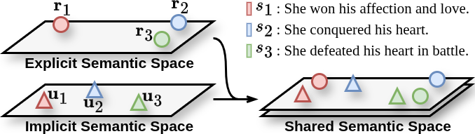
Figure 1: Overview of DualCSE. The explicit and implicit semantic spaces are combined into a shared space.

To evaluate the capability of DualCSE in capturing inter-sentence and intra-sentence relations, we conduct two experiments of two tasks: Recognizing Textual Entailment (RTE) and Estimating Implicitness Score (EIS). Experimental results show that DualCSE captures inter- and intra-sentence relations more accurately than conventional methods.

2 Implied NLI (INLI) Dataset

The INLI dataset (Havaldar et al., 2025) is used for DualCSE. As shown in Table 1, the INLI dataset differs from standard NLI datasets such as SNLI (Bowman et al., 2015) and MNLI (Williams et al., 2018) in that it provides four different hypotheses, labeled with “implied-entailment”, “explicit-entailment”, “neutral”, and “contradiction” for a single premise. The implied-entailment and explicit-entailment indicate entailment with respect to the implicit and explicit semantics of the premise, respectively.

Premise

Diane says, “Would you like to go a party tonight?”

Sophie responds, “I am too tired.”

Implied Entailment

Sophie would prefer not to attend the party this evening.

Explicit Entailment

Sophie claims to be too tired.

Neutral

The party will take place outside.

Contradiction

Sophie is excited to attend the party this evening.

Table 1: An example of a sample in the INLI dataset

3 DualCSE

This section presents DualCSE, a method that encodes each sentence $s$ into two embeddings: $\mathbf{r}$, representing its explicit semantics and $\mathbf{u}$, representing its implicit semantics. The loss function for learning these embeddings is first explained, followed by a description of the model architecture.

3.1 Contrastive Loss

For a given sample in the INLI dataset, let $s_{i}$ be a premise, and $s^{+}_{i1}$, $s^{+}_{i2}$, and $s^{-}_{i}$ be the explicit-entailment, implied-entailment, and contradiction hypothesis for $s_{i}$, respectively. The explicit-semantic embeddings are denoted as $\mathbf{r}_{i}$, $\mathbf{r}^{+}_{i1}$, $\mathbf{r}^{+}_{i2}$, and $\mathbf{r}^{-}_{i}$, while the implicit-semantic embeddings are denoted as $\mathbf{u}_{i}$, $\mathbf{u}^{+}_{i1}$, $\mathbf{u}^{+}_{i2}$, and $\mathbf{u}^{-}_{i}$. The contrastive loss $l_{i}$ for $i$-th instance in a batch of size $N$ is calculated as follows:

$$v(\mathbf{h}_{1},\mathbf{h}_{2})=e^{\mathrm{sim}(\mathbf{h}_{1},\mathbf{h}_{2})/\tau},$$ (1)

$$\begin{array}[b]{@{}l@{}}l_{i}=\\ \displaystyle-\log{\frac{v(\mathbf{r}_{i},\mathbf{r}^{+}_{i1})}{\sum^{N}_{j=1}(v(\mathbf{r}_{i},\mathbf{r}^{+}_{j1})+v(\mathbf{r}_{i},\mathbf{r}^{-}_{j})+v(\mathbf{r}_{i},\mathbf{u}_{j}))}}\\ \displaystyle-\log{\frac{v(\mathbf{u}_{i},\mathbf{r}^{+}_{i2})}{\sum^{N}_{j=1}(v(\mathbf{u}_{i},\mathbf{r}^{+}_{j2})+v(\mathbf{u}_{i},\mathbf{r}^{-}_{j})+v(\mathbf{u}_{i},\mathbf{r}_{j}))}}\\ \displaystyle-\log{\frac{v(\mathbf{r}^{+}_{i1},\mathbf{u}^{+}_{i1})}{\sum^{N}_{j=1}v(\mathbf{r}^{+}_{i1},\mathbf{u}^{+}_{j1})}}-\log{\frac{v(\mathbf{r}^{+}_{i2},\mathbf{u}^{+}_{i2})}{\sum^{N}_{j=1}v(\mathbf{r}^{+}_{i2},\mathbf{u}^{+}_{j2})}}\\ \displaystyle-\log{\frac{v(\mathbf{r}^{-}_{i},\mathbf{u}^{-}_{i})}{\sum^{N}_{j=1}v(\mathbf{r}^{-}_{i},\mathbf{u}^{-}_{j})}},\end{array}$$ (2)

where $\mathrm{sim}(\mathbf{h}_{1},\mathbf{h}_{2})$ denotes the cosine similarity between $\mathbf{h}_{1}$ and $\mathbf{h}_{2}$, and $\tau$ is the temperature parameter. Intuitively, as shown in Figure 2, the pairs ($\mathbf{r}_{i}$, $\mathbf{r}^{+}_{i1}$) and ($\mathbf{u}_{i}$, $\mathbf{r}^{+}_{i2}$) are encouraged to close together, whereas the pairs ($\mathbf{r}_{i}$, $\mathbf{r}^{-}_{i}$) and ($\mathbf{u}_{i}$, $\mathbf{r}^{-}_{i}$) are encouraged to push apart. These are designed to capture inter-sentence relations, i.e., a premise and entailment hypothesis are similar, while a premise and contradiction hypothesis are dissimilar. Furthermore, the pairs ($\mathbf{r}^{+}_{i1}$, $\mathbf{u}^{+}_{i1}$), ($\mathbf{r}^{+}_{i2}$, $\mathbf{u}^{+}_{i2}$), and ($\mathbf{r}^{-}_{i}$, $\mathbf{u}^{-}_{i}$) are encouraged to close together, whereas the pair ($\mathbf{r}_{i}$, $\mathbf{u}_{i}$) is encouraged to push apart. These are designed to capture intra-sentence relations under the assumption that the hypotheses in the INLI dataset are less ambiguous and convey more similar explicit and implicit semantics than a premise.

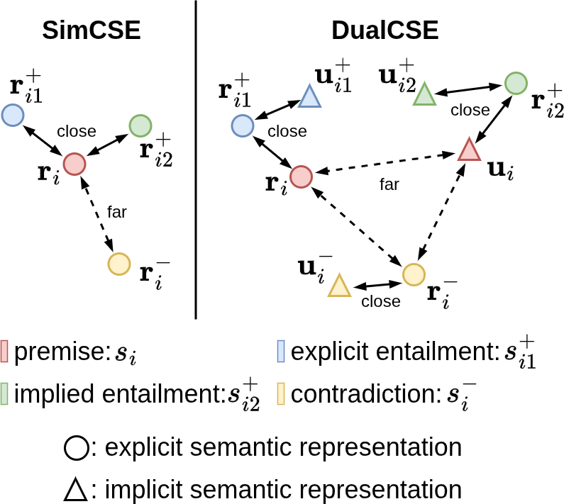
Figure 2: Conceptual diagram of contrastive loss in SimCSE (Gao et al., 2021) and our DualCSE.

3.2 Model Architecture

This study employs two types of encoder models as follows.

Cross-encoder

A single BERT (Devlin et al., 2019) or RoBERTa (Liu et al., 2019) model that outputs the representation $\mathbf{r}$ for the explicit semantic of $s$ when given the input “[CLS] $s$ [SEP] explicit,” and $\mathbf{u}$ for the implicit semantic of $s$ when given the input “[CLS] $s$ [SEP] implicit.”

Bi-encoder

Two separate BERT or RoBERTa models are trained to obtain $\mathbf{r}$ and $\mathbf{u}$, respectively.

For both models, the hidden state of the final layer of [CLS] is used as the sentence embedding.

4 Experiments

We validate the effectiveness of DualCSE through experiments on two tasks. The first task is Recognizing Textual Entailment (RTE), which involves the model’s capacity to correctly capture entailment relationships between sentences. The second task is Estimating Implicitness Score (EIS), which aims to estimate the extent to which an implicit meaning deviates from a literal meaning.

4.1 Experimental Setup

For the two model architectures of DualCSE, the pre-trained BERT_base and RoBERTa_base are employed as the encoder models. Only the settings and results of the RoBERTa model are reported in this section, since it demonstrated higher performance than BERT on the development set. The batch size and learning rate are optimized using the development set, resulting in 64 and 5e-5 for the cross-encoder, and 32 and 3e-5 for the bi-encoder. The temperature parameter $\tau$ is set to 0.05, following Gao et al. (2021) and Yoda et al. (2024).

4.2 Recognizing Textual Entailment (RTE)

Task definition

RTE is a task that classifies a given premise and hypothesis pair ($p$, $h$) as either “entailment” or “non-entailment.” The INLI dataset (Havaldar et al., 2025) is used for the experiment, where the neutral and contradiction labels are converted to “non-entailment,” and both explicit and implied entailment are retained as “entailment.”

Method

Let $\mathbf{r}_{1}$ and $\mathbf{r}_{2}$ be the representations of the explicit semantics of the premise $p$ and hypothesis $h$, respectively, and $\mathbf{u}_{1}$ be the representation of the implicit semantics of $p$. DualCSE predicts that $p$ and $h$ are in an entailment relation if

$$\max\bigl(\cos(\mathbf{r}_{1},\mathbf{r}_{2}),\cos(\mathbf{u}_{1},\mathbf{r}_{2})\bigr)>\gamma,$$ (3)

and predicts non-entailment otherwise. The threshold $\gamma$ is tuned on the INLI development set.

Baselines

Two baselines are compared to DualCSE: SimCSE (SNLI+MNLI) (Gao et al., 2021) and SimCSE (INLI). The latter is a SimCSE model trained on the INLI dataset. These baselines predict labels using the same approach as our model, which involves determining whether the cosine similarity between the premise and hypothesis embeddings exceeds the threshold. Additionally, for reference, we also provide the results of a few-shot setting with large language models (LLMs).

Model	Exp.	Imp.	Neu.	Con.	Avg.
SimCSE (SNLI+MNLI)	79.80	49.00	74.30	67.60	67.68
SimCSE (INLI)	90.60	69.10	66.90	91.00	79.40
DualCSE-Cross (ours)	90.20	73.40	68.40	88.70	80.18
DualCSE-Bi (ours)	91.90	69.90	72.10	87.60	80.38
Gemini-1.5-Pro	97.90	80.30	92.00	95.40	91.40

Table 2: Results of RTE task (accuracy %). Exp., Imp., Neu., and Con. mean the accuracy for the instances where the original label is explicit-entailment, implied-entailment, neutral, and contradiction, respectively.

Query: Madeleine has just moved into a neighbourhood and meets her new neighbour Pierre.
Pierre says, “Are you from this state?” Madeleine responds, “I’m from Oregon.”
Explicit semantic: Madeleine is from Oregon.	Implicit semantic: Madeleine was born in a different state.
#1 Laverne moved from Canada.	#1 The place does not belong to Quincy.
#2 Angela and her family live in Portland now.	#2 Madeleine enjoys food with some spice, but not if it’s overly hot.
#3 Alyce works in Portland.	#3 Earlene is not originally from this area.

Table 3: An example of a simple retrieval experiment. Explicit semantic and Implicit semantic are the explicit-entailment and implied-entailment hypotheses in the INLI dataset, respectively. These are not used as a query for sentence retrieval.

Results

The results are shown in Table 2. First, the proposed method DualCSE outperforms SimCSE (INLI) in both model architectures, demonstrating the effectiveness of representations for the explicit and implicit semantics of sentences. Next, SimCSE (SNLI+MNLI) has the largest gap in accuracy between Exp. and Imp. This is likely due to SNLI and MNLI containing relatively few sentences with implicit semantics, as reported by Havaldar et al. (2025). Finally, LLMs generally demonstrate superior performance compared to the encoder models. However, similar to other models, LLMs consistently show a tendency toward lower performance on Imp. compared to Exp.

4.3 Estimating Implicitness Score (EIS)

Task definition

Given two sentences $s_{1}$ and $s_{2}$, predict which sentence exhibits a higher degree of implicitness. Two datasets are employed for this task: the INLI (Havaldar et al., 2025) and the dataset provided by Wang et al. (2025). For the INLI, it is supposed that the premise is more implicit than the hypothesis.

Method

The implicitness score of a sentence $s$ is calculated as follows:

$$\mathrm{imp}(s)=1-\cos(\mathbf{r},\mathbf{u}).$$ (4)

We predict which of the sentences $s_{1}$ and $s_{2}$ has the greater implicitness score:

$$\arg\max\bigl(\mathrm{imp}(s_{1}),\mathrm{imp}(s_{2})\bigr).$$ (5)

Baselines

Three baselines are compared in this experiment: (1) Length, which chooses the longer sentence, (2) ImpScore (original) (Wang et al., 2025), and (3) ImpScore (INLI), which is the ImpScore trained on the INLI dataset using RoBERTa as the encoder model.

Model	INLI	Wang et al. (2025)
Length	99.90	73.37
ImpScore (original)	80.55	95.20
ImpScore (INLI)	99.97	81.56
DualCSE-Cross (ours)	99.97	79.31
DualCSE-Bi (ours)	100	77.48

Table 4: ESI task results (accuracy %)

Results

The results are shown in Table 4. First, DualCSE achieves near-perfect accuracy in both model architectures for the INLI dataset, i.e., for the in-domain setting. However, this may be because the length ratio of the input sentence pairs serves as a useful signal, as evidenced by the near-perfect performance accuracy achieved by Length as well. Next, in the out-of-domain setting (Wang’s dataset), the accuracy of DualCSE and ImpScore (INLI) decreases to nearly 80%. The performance of DualCSE is comparable to that of ImpScore. It is worth noting that the ImpScore has been developed specifically for the purpose of predicting the implicitness score, whereas our DualCSE is capable of generating embeddings for both explicit and implicit semantics, which enables it to perform other downstream tasks.

5 Analysis

Loss function	RTE	EIS
DualCSE-Cross	80.18	99.97
w/o contradiction	64.57	99.88
w/o intra sentence	80.10	92.25
w/o contradiction & intra sentence	64.68	32.75

Table 5: Ablation results (accuracy %)

Ablation Study

The ablation study is conducted to investigate the contributions of the components of the proposed contrastive loss. We train the models in three scenarios: excluding the loss for contradiction hypotheses, excluding the loss for intra-sentence relations, and excluding both. As shown in Table 5, the loss for contradiction hypotheses is more effective for the RTE task, while the loss for intra-sentence relations is more effective for the EIS task.

Retrieval Experiment

A qualitative evaluation of the explicit and implicit embeddings is conducted through a simple search experiment. Specifically, we select several premises from the development data of INLI as queries and retrieve the top three similar hypotheses from the training data that most closely match the explicit and implicit semantics of each query. As shown in Table 3, DualCSE facilitates a separate search for the sentences that correspond to explicit and implicit semantics.

6 Conclusion

This paper proposed DualCSE, a sentence embedding method that assigns two representations for the explicit and implicit semantics of sentences. The experimental results of the RTE and EIS tasks demonstrated DualCSE successfully encoded literal and latent meanings into separate embeddings.

Limitations

We use only the INLI (Havaldar et al., 2025) dataset for the training. However, the variation of the sentences in the INLI is rather limited. It is important to apply DualCSE to the training data of various domains. For example, the datasets for hate speech detection (Hartvigsen et al., 2022) and sentiment analysis (Pontiki et al., 2014) are converted to the INLI format and can be used as the training data.

This study conducted a simple retrieval experiment with the aim of applying it to real-world applications. In the future, it would be desirable to apply our method to more practical settings, such as analyzing customer reviews and implementing search engines.

Recently, sentence embedding methods using LLMs have been actively studied (BehnamGhader et al., 2024; Jiang et al., 2024; Yamada and Zhang, 2025). Extending our method to LLMs is another future direction.

Appendix A Dataset Statistics

Table 6 shows the statistics of the INLI dataset and Wang’s dataset (Wang et al., 2025).

Dataset	train	development	test
INLI	32,000	4,000	4,000
Wang et al. (2025)	101,320	5,630	5,630

Table 6: Statistics of datasets. This table shows the number of premise-hypothesis pairs for the INLI dataset and that of implicit-explicit sentence pairs for Wang’s dataset.

batch size	learning rate
	1e-5	3e-5	5e-5
16	76.50	77.10	77.53
32	76.40	77.42	77.70
64	75.42	76.92	77.45

(a) DualCSE-Cross-BERT

batch size	learning rate
	1e-5	3e-5	5e-5
16	76.92	78.57	78.30
32	76.23	78.07	78.47
64	75.45	77.25	77.97

(b) DualCSE-Bi-BERT

batch size	learning rate
	1e-5	3e-5	5e-5
16	80.50	80.60	80.58
32	79.85	80.75	81.12
64	78.83	79.93	81.15

(c) DualCSE-Cross-RoBERTa

batch size	learning rate
	1e-5	3e-5	5e-5
16	80.40	80.45	80.33
32	80.60	80.80	80.45
64	79.47	80.55	80.65

(d) DualCSE-Bi-RoBERTa

batch size	learning rate
	1e-5	3e-5	5e-5
16	76.38	76.82	76.63
32	76.65	77.35	77.25
64	75.65	76.40	76.40

(e) SimCSE-BERT

batch size	learning rate
	1e-5	3e-5	5e-5
16	80.12	79.18	78.30
32	79.52	80.43	79.72
64	79.43	79.85	79.37

(f) SimCSE-RoBERTa

Table 7: Grid search results

Appendix B Hyperparameter Optimization

The hyperparameters, i.e., batch size and learning rate, are optimized via a grid search. The results of the grid search are shown in Table 7. All experiments were conducted on a 20 GB NVIDIA H100 MIG instance (a quarter of a full H100). The training times are approximately 30, 16, and 9 minutes for batch sizes of 16, 32, and 64, respectively.

Appendix C Prompt

The prompt used for the RTE task is shown in Figure 3, which is shared across the following LLMs: GPT-4, GPT-4o, GPT-4o-mini, Claude-3.7-Sonnet, Gemini-1.5-Pro, Gemini-2.0-Flash, DeepSeek-v3 and Mistral-Large. For each test data point, eight sentence pairs are randomly selected from the training data and included in the prompt for few-shot learning, with an equal number of entailment and non-entailment pairs.

Figure 3: Prompt template for RTE task.

Appendix D Full Results of RTE

The full results of the RTE task are shown in Table 8.

Model	Exp.	Imp.	Neu.	Con.	Avg.
LLMs
GPT-4	98.40	83.10	88.90	94.10	91.12
GPT-4o	98.30	84.50	87.20	94.30	91.08
GPT-4o-mini	97.30	74.30	90.30	94.40	89.08
Gemini-1.5-Pro	97.90	80.30	92.00	95.40	91.40
Gemini-2.0-Flash	98.20	85.50	85.40	93.40	90.62
Claude-3.7-Sonnet	97.10	75.90	93.00	95.90	90.47
DeepSeek-v3	99.10	85.20	87.40	93.30	91.25
Mistral Large	98.10	81.30	88.70	94.60	90.68
BERT-based
SimCSE (SNLI+MNLI)	78.50	41.00	77.40	67.50	66.10
SimCSE (INLI)	89.80	67.60	65.70	83.90	76.75
ImpScore (INLI)	59.20	26.30	75.30	81.50	60.58
DualCSE-Cross (ours)	86.80	64.30	72.40	87.50	77.75
DualCSE-Bi (ours)	91.30	63.30	73.60	85.10	78.32
RoBERTa-based
SimCSE (SNLI+MNLI)	79.80	49.00	74.30	67.60	67.68
SimCSE (INLI)	90.60	69.10	66.90	91.00	79.40
ImpScore (INLI)	81.60	56.80	47.70	61.60	61.92
DualCSE-Cross (ours)	90.20	73.40	68.40	88.70	80.18
DualCSE-Bi (ours)	91.90	69.90	72.10	87.60	80.38

Table 8: Full results of the RTE task (accuracy %)

Appendix E Full Results of EIS

The full results of the EIS task are shown in Table 9. It is noteworthy that DualCSE-Cross outperforms ImpScore (INLI) when BERT is used as the base encoder, whereas they are comparable when RoBERTa is used.

Model	INLI	Wang et al. (2025)
Length	99.90	73.37
ImpScore (original)	80.55	95.20
BERT-based
ImpScore (INLI)	99.97	76.91
DualCSE-Cross (ours)	100	80.46
DualCSE-Bi (ours)	99.97	79.88
RoBERTa-based
ImpScore (INLI)	99.97	81.56
DualCSE-Cross (ours)	99.97	79.31
DualCSE-Bi (ours)	100	77.48

Table 9: Full results of the EIS task (accuracy %)

Appendix F Ablation Details

The detail description of ablation experiments are follows.

w/o contradiction

We remove $v(\mathbf{r}_{i},\mathbf{r}^{-}_{j})$ and $v(\mathbf{u}_{i},\mathbf{r}^{-}_{j})$ in the denominator and $-\log{\frac{v(\mathbf{r}^{-}_{i},\mathbf{u}^{-}_{i})}{\sum^{N}_{j=1}v(\mathbf{r}^{-}_{i},\mathbf{u}^{-}_{j})}}$ from Equation (2). The entire formula is as follows:

$$\begin{array}[b]{@{}l@{}}l_{i}=\\ \displaystyle-\log{\frac{v(\mathbf{r}_{i},\mathbf{r}^{+}_{i1})}{\sum^{N}_{j=1}(v(\mathbf{r}_{i},\mathbf{r}^{+}_{j1})+v(\mathbf{r}_{i},\mathbf{u}_{j}))}}\\ \displaystyle-\log{\frac{v(\mathbf{u}_{i},\mathbf{r}^{+}_{i2})}{\sum^{N}_{j=1}(v(\mathbf{u}_{i},\mathbf{r}^{+}_{j2})+v(\mathbf{u}_{i},\mathbf{r}_{j}))}}\\ \displaystyle-\log{\frac{v(\mathbf{r}^{+}_{i1},\mathbf{u}^{+}_{i1})}{\sum^{N}_{j=1}v(\mathbf{r}^{+}_{i1},\mathbf{u}^{+}_{j1})}}-\log{\frac{v(\mathbf{r}^{+}_{i2},\mathbf{u}^{+}_{i2})}{\sum^{N}_{j=1}v(\mathbf{r}^{+}_{i2},\mathbf{u}^{+}_{j2})}}.\end{array}$$ (6)

w/o intra-sentence

We remove $v(\mathbf{r}_{i},\mathbf{u}_{j})$ and $v(\mathbf{u}_{i},\mathbf{r}_{j})$ in the denominator and $-\log{\frac{v(\mathbf{r}^{+}_{i1},\mathbf{u}^{+}_{i1})}{\sum^{N}_{j=1}v(\mathbf{r}^{+}_{i1},\mathbf{u}^{+}_{j1})}}$, $-\log{\frac{v(\mathbf{r}^{+}_{i2},\mathbf{u}^{+}_{i2})}{\sum^{N}_{j=1}v(\mathbf{r}^{+}_{i2},\mathbf{u}^{+}_{j2})}}$ and $-\log{\frac{v(\mathbf{r}^{-}_{i},\mathbf{u}^{-}_{i})}{\sum^{N}_{j=1}v(\mathbf{r}^{-}_{i},\mathbf{u}^{-}_{j})}}$ from Equation (2). The entire formula is as follows:

$$\begin{array}[b]{@{}l@{}}l_{i}=\\ \displaystyle-\log{\frac{v(\mathbf{r}_{i},\mathbf{r}^{+}_{i1})}{\sum^{N}_{j=1}(v(\mathbf{r}_{i},\mathbf{r}^{+}_{j1})+v(\mathbf{r}_{i},\mathbf{r}^{-}_{j}))}}\\ \displaystyle-\log{\frac{v(\mathbf{u}_{i},\mathbf{r}^{+}_{i2})}{\sum^{N}_{j=1}(v(\mathbf{u}_{i},\mathbf{r}^{+}_{j2})+v(\mathbf{u}_{i},\mathbf{r}^{-}_{j}))}}.\end{array}$$ (7)

w/o contradiction & intra-sentence

The formula of the loss function is as follows:

$$\begin{array}[b]{@{}l@{}}l_{i}=\\ \displaystyle-\log{\frac{v(\mathbf{r}_{i},\mathbf{r}^{+}_{i1})}{\sum^{N}_{j=1}(v(\mathbf{r}_{i},\mathbf{r}^{+}_{j1}))}}\\ \displaystyle-\log{\frac{v(\mathbf{u}_{i},\mathbf{r}^{+}_{i2})}{\sum^{N}_{j=1}(v(\mathbf{u}_{i},\mathbf{r}^{+}_{j2}))}}.\end{array}$$ (8)

The full results of the ablation experiments are shown in Table 10.

Loss function	RTE	EIS
DualCSE-Cross-BERT	77.75	100
w/o contradiction	64.13	99.90
w/o intra sentence	77.50	47.13
w/o contradiction & intra sentence	64.38	31.83
DualCSE-Bi-BERT	78.32	99.97
w/o contradiction	65.97	100
w/o intra sentence	77.30	63.42
w/o contradiction & intra sentence	65.47	81.35
DualCSE-Cross-RoBERTa	80.18	99.97
w/o contradiction	64.57	99.88
w/o intra sentence	80.10	92.25
w/o contradiction & intra sentence	64.68	32.75
DualCSE-Bi-RoBERTa	80.38	100
w/o contradiction	66.13	99.95
w/o intra sentence	80.57	60.35
w/o contradiction & intra sentence	65.07	76.15

Table 10: Full results of ablation experiments

Appendix G Examples of Retrieval Experiment

Several examples of the retrieval experiment are shown in Table 11.

Query: Joseph wants to know about Fred’s food preferences. Joseph says, “Would you be into eating at a diner with burgers?” Fred responds, “I want to get a salad.”
Explicit semantic: Fred wants to get a salad.	Implicit semantic: It’s unlikely that Fred wants to eat burgers at a diner.
#1 Terrie prefers salads (to food served at fast food restaurants).	#1 Cookies are something that Fred enjoys.
#2 Hannah will travel up to five miles, but only for a salad.	#2 Fredrick enjoys spicy food, but only if he has milk to cool his mouth.
#3 Marcus says, “That’d be great,” in response to Normand’s suggestion of a vegetarian restaurant.	#3 Freddie believes that pizza would be a good food choice.

(a) Example #1

Query: Pete says, “That chocolate cake looks delicious. Aren’t you going to have some with me?” Connie responds, “I am allergic to chocolate.”
Explicit semantic: Connie claims to have an allergy to chocolate.	Implicit semantic: Connie will not join Pete in eating chocolate cake.
#1 Francisco says, “It is too cold,” when Vickie asks if he wants to go swimming.	#1 Francis cannot eat certain foods.
#2 Christie says that she and Peter are completely different.	#2 Elva won’t eat any cake.
#3 Katie doesn’t like the thing that Cristina is talking about.	#3 Carmen prefers not to eat at the restaurant.

(b) Example #2

Query: Phoebe says, “Do you like my new outfit?” Rolland responds, “You shouldn’t be allowed to buy clothes.”
Explicit semantic: Rolland believes Phoebe should be prevented from purchasing clothes.	Implicit semantic: Rolland really hates Phoebe’s new outfit.
#1 Rosendo claims he did not order the code red.	#1 The item is too big for her, so it won’t be suitable.
#2 Rolland does not have any children.	#2 Alphonso will not be going shopping.
#3 Rosendo doesn’t think listening to local indie artists is cool.	#3 Lois has no desire to go to the mall.

(c) Example #3

Table 11: Several examples of a simple retrieval experiment

References

- BehnamGhader et al. (2024) Parishad BehnamGhader, Vaibhav Adlakha, Marius Mosbach, Dzmitry Bahdanau, Nicolas Chapados, and Siva Reddy. 2024. LLM2vec: Large language models are secretly powerful text encoders. In First Conference on Language Modeling.
- Bowman et al. (2015) Samuel R. Bowman, Gabor Angeli, Christopher Potts, and Christopher D. Manning. 2015. A large annotated corpus for learning natural language inference. In Proceedings of the 2015 Conference on Empirical Methods in Natural Language Processing, pages 632–642, Lisbon, Portugal. Association for Computational Linguistics.
- Chen et al. (2020) Ting Chen, Simon Kornblith, Mohammad Norouzi, and Geoffrey Hinton. 2020. A simple framework for contrastive learning of visual representations. In Proceedings of the 37th International Conference on Machine Learning, volume 119 of Proceedings of Machine Learning Research, pages 1597–1607. PMLR.
- Devlin et al. (2019) Jacob Devlin, Ming-Wei Chang, Kenton Lee, and Kristina Toutanova. 2019. BERT: Pre-training of deep bidirectional transformers for language understanding. In Proceedings of the 2019 Conference of the North American Chapter of the Association for Computational Linguistics: Human Language Technologies, Volume 1 (Long and Short Papers), pages 4171–4186, Minneapolis, Minnesota. Association for Computational Linguistics.
- Gao et al. (2021) Tianyu Gao, Xingcheng Yao, and Danqi Chen. 2021. SimCSE: Simple contrastive learning of sentence embeddings. In Proceedings of the 2021 Conference on Empirical Methods in Natural Language Processing, pages 6894–6910, Online and Punta Cana, Dominican Republic. Association for Computational Linguistics.
- Hartvigsen et al. (2022) Thomas Hartvigsen, Saadia Gabriel, Hamid Palangi, Maarten Sap, Dipankar Ray, and Ece Kamar. 2022. ToxiGen: A large-scale machine-generated dataset for adversarial and implicit hate speech detection. In Proceedings of the 60th Annual Meeting of the Association for Computational Linguistics (Volume 1: Long Papers), pages 3309–3326, Dublin, Ireland. Association for Computational Linguistics.
- Havaldar et al. (2025) Shreya Havaldar, Hamidreza Alvari, John Palowitch, Mohammad Javad Hosseini, Senaka Buthpitiya, and Alex Fabrikant. 2025. Entailed between the lines: Incorporating implication into NLI. In Proceedings of the 63rd Annual Meeting of the Association for Computational Linguistics (Volume 1: Long Papers), pages 32274–32290, Vienna, Austria. Association for Computational Linguistics.
- Jiang et al. (2024) Ting Jiang, Shaohan Huang, Zhongzhi Luan, Deqing Wang, and Fuzhen Zhuang. 2024. Scaling sentence embeddings with large language models. In Findings of the Association for Computational Linguistics: EMNLP 2024, pages 3182–3196, Miami, Florida, USA. Association for Computational Linguistics.
- Jiang et al. (2022) Ting Jiang, Jian Jiao, Shaohan Huang, Zihan Zhang, Deqing Wang, Fuzhen Zhuang, Furu Wei, Haizhen Huang, Denvy Deng, and Qi Zhang. 2022. PromptBERT: Improving BERT sentence embeddings with prompts. In Proceedings of the 2022 Conference on Empirical Methods in Natural Language Processing, pages 8826–8837, Abu Dhabi, United Arab Emirates. Association for Computational Linguistics.
- Li and Li (2024) Xianming Li and Jing Li. 2024. AoE: Angle-optimized embeddings for semantic textual similarity. In Proceedings of the 62nd Annual Meeting of the Association for Computational Linguistics (Volume 1: Long Papers), pages 1825–1839, Bangkok, Thailand. Association for Computational Linguistics.
- LI et al. (2025) Xianming LI, Zongxi Li, Jing Li, Haoran Xie, and Qing Li. 2025. ESE: Espresso sentence embeddings. In The Thirteenth International Conference on Learning Representations.
- Liu et al. (2019) Yinhan Liu, Myle Ott, Naman Goyal, Jingfei Du, Mandar Joshi, Danqi Chen, Omer Levy, Mike Lewis, Luke Zettlemoyer, and Veselin Stoyanov. 2019. Roberta: A robustly optimized bert pretraining approach. Preprint, arXiv:1907.11692.
- Maas et al. (2011) Andrew L. Maas, Raymond E. Daly, Peter T. Pham, Dan Huang, Andrew Y. Ng, and Christopher Potts. 2011. Learning word vectors for sentiment analysis. In Proceedings of the 49th Annual Meeting of the Association for Computational Linguistics: Human Language Technologies, pages 142–150, Portland, Oregon, USA. Association for Computational Linguistics.
- Muennighoff et al. (2023) Niklas Muennighoff, Nouamane Tazi, Loic Magne, and Nils Reimers. 2023. MTEB: Massive text embedding benchmark. In Proceedings of the 17th Conference of the European Chapter of the Association for Computational Linguistics, pages 2014–2037, Dubrovnik, Croatia. Association for Computational Linguistics.
- Ni et al. (2022) Jianmo Ni, Gustavo Hernandez Abrego, Noah Constant, Ji Ma, Keith Hall, Daniel Cer, and Yinfei Yang. 2022. Sentence-t5: Scalable sentence encoders from pre-trained text-to-text models. In Findings of the Association for Computational Linguistics: ACL 2022, pages 1864–1874, Dublin, Ireland. Association for Computational Linguistics.
- Pontiki et al. (2014) Maria Pontiki, Dimitris Galanis, John Pavlopoulos, Harris Papageorgiou, Ion Androutsopoulos, and Suresh Manandhar. 2014. SemEval-2014 task 4: Aspect based sentiment analysis. In Proceedings of the 8th International Workshop on Semantic Evaluation (SemEval 2014), pages 27–35, Dublin, Ireland. Association for Computational Linguistics.
- Reimers and Gurevych (2019) Nils Reimers and Iryna Gurevych. 2019. Sentence-BERT: Sentence embeddings using Siamese BERT-networks. In Proceedings of the 2019 Conference on Empirical Methods in Natural Language Processing and the 9th International Joint Conference on Natural Language Processing (EMNLP-IJCNLP), pages 3982–3992, Hong Kong, China. Association for Computational Linguistics.
- Sun et al. (2025) Yiqun Sun, Qiang Huang, Anthony K. H. Tung, and Jun Yu. 2025. Text embeddings should capture implicit semantics, not just surface meaning. Preprint, arXiv:2506.08354.
- Thakur et al. (2021) Nandan Thakur, Nils Reimers, Andreas Rücklé, Abhishek Srivastava, and Iryna Gurevych. 2021. BEIR: A heterogeneous benchmark for zero-shot evaluation of information retrieval models. In Thirty-fifth Conference on Neural Information Processing Systems Datasets and Benchmarks Track (Round 2).
- Wang et al. (2024) Liang Wang, Nan Yang, Xiaolong Huang, Binxing Jiao, Linjun Yang, Daxin Jiang, Rangan Majumder, and Furu Wei. 2024. Text embeddings by weakly-supervised contrastive pre-training. Preprint, arXiv:2212.03533.
- Wang et al. (2025) Yuxin Wang, Xiaomeng Zhu, Weimin Lyu, Saeed Hassanpour, and Soroush Vosoughi. 2025. Impscore: A learnable metric for quantifying the implicitness level of sentences. In The Thirteenth International Conference on Learning Representations.
- Williams et al. (2018) Adina Williams, Nikita Nangia, and Samuel Bowman. 2018. A broad-coverage challenge corpus for sentence understanding through inference. In Proceedings of the 2018 Conference of the North American Chapter of the Association for Computational Linguistics: Human Language Technologies, Volume 1 (Long Papers), pages 1112–1122, New Orleans, Louisiana. Association for Computational Linguistics.
- Yamada and Zhang (2025) Kosuke Yamada and Peinan Zhang. 2025. Out-of-the-box conditional text embeddings from large language models. Preprint, arXiv:2504.16411.
- Yoda et al. (2024) Shohei Yoda, Hayato Tsukagoshi, Ryohei Sasano, and Koichi Takeda. 2024. Sentence representations via Gaussian embedding. In Proceedings of the 18th Conference of the European Chapter of the Association for Computational Linguistics (Volume 2: Short Papers), pages 418–425, St. Julian’s, Malta. Association for Computational Linguistics.
- Zhang et al. (2025) Dun Zhang, Jiacheng Li, Ziyang Zeng, and Fulong Wang. 2025. Jasper and stella: distillation of sota embedding models. Preprint, arXiv:2412.19048.
- Zhang et al. (2024) Xin Zhang, Yanzhao Zhang, Dingkun Long, Wen Xie, Ziqi Dai, Jialong Tang, Huan Lin, Baosong Yang, Pengjun Xie, Fei Huang, Meishan Zhang, Wenjie Li, and Min Zhang. 2024. mGTE: Generalized long-context text representation and reranking models for multilingual text retrieval. In Proceedings of the 2024 Conference on Empirical Methods in Natural Language Processing: Industry Track, pages 1393–1412, Miami, Florida, US. Association for Computational Linguistics.