Systematics on two-body mass measurements and the $\Lambda$-baryon mass

Abstract

The effect of detector-related uncertainties on the determination of the parent particle mass in two-body decays is described. Studies of the biases versus the sum and difference of the daughter particle momenta can be used to determine biases on the mass. The approach is illustrated for the case of measuring the $\Lambda$ hyperon mass.

Keywords: Particle tracking detectors; Analysis and statistical methods

1 Introduction

Detailed understanding of systematic uncertainties in the tracking of charged particles is essential for an accurate determination of particle masses and for understanding the performance of forward spectrometers. This paper discusses how detector-related biases, such as those affecting the charged-particle momentum scale and ionization energy loss, influence mass measurements for two-body decay processes. Ideally, these effects would be modelled and corrected by the detector alignment and calibration procedure. This is not always possible, necessitating ad hoc corrections at later stages of the analysis chain. By formulating the corrections in terms of physical parameters, such studies can provide feedback to improve the detector modelling. Although the formalism developed is general, as a specific example, the measurement of the mass of the $\Lambda$ hyperon from its decay to the ${\mathrm{p}}\pi^{-}$ final state is discussed and motivated. For this mode, the topologically similar decay mode ${{\mathrm{K}}^{0}_{\mathrm{S}}}\!\rightarrow{{\pi}^{+}}{{\pi}^{-}}$ is an ideal calibration channel, as it is more sensitive to detector biases. Experimental measurements of the $\Lambda$ mass can be compared to lattice QCD predictions [1]. In addition, comparing the masses of the ${\Lambda}$ and $\overline{{\Lambda}}$ hyperons provides a test of CPT-symmetry [2].

This paper is structured as follows. First, the current knowledge of the ${\Lambda}$ mass is discussed, and it is argued that new measurements are needed. The remainder of the paper describes the experimental challenges to such a measurement. Section 3 describes the simulation used for these studies. Following this, in Section 4 the formalism used is detailed. Section 5 shows how the ${\mathrm{K}}^{0}_{\mathrm{S}}$ decay can be used to calibrate the measured momenta and allow the ${\Lambda}$ mass to be measured.

2 Current knowledge of the ${\Lambda}$ mass

The 2024 Review of Particle Properties, the PDG [3], reports $m_{{\Lambda}}=1115.683\pm 0.006\,\textrm{MeV}/c^{2}$ [3]. This value is based on data collected in the 1990s at the Brookhaven AGS by the E766 collaboration [4]. The PDG value is the weighted average of the values $m_{{\Lambda}}=1115.678\pm 0.006\,\textrm{(stat)}\,\pm\,0.006\,\textrm{(syst)}\,\textrm{MeV}/c^{2}$ and $m_{{\kern 0.0pt\overline{\kern 0.0pt\Lambda}}}=1115.690\pm 0.008\,\textrm{(stat)}\,\pm\,0.006\,\textrm{(syst)}\,\textrm{MeV}/c^{2}$ reported in [4] under the assumption that the systematic uncertainties are not correlated. As the systematic uncertainty is entirely due to the knowledge of the ${\mathrm{K}}^{0}_{\mathrm{S}}$ mass used to calibrate the momentum scale, this procedure is questionable. Furthermore, the uncertainty on the ${\mathrm{K}}^{0}_{\mathrm{S}}$ mass has improved from $m_{{{\mathrm{K}}^{0}_{\mathrm{S}}}}=497.671\pm 0.031\,\textrm{MeV}/c^{2}$ used in [4] to $m_{{{\mathrm{K}}^{0}_{\mathrm{S}}}}=497.611\pm 0.013\,\textrm{MeV}/c^{2}$ quoted by the PDG [3]. There is sufficient information in [4] to recalculate $m_{{\Lambda}}$ to account for the change in $m_{{{\mathrm{K}}^{0}_{\mathrm{S}}}}$. The updated weighted average, with the assumption of fully correlated systematic uncertainties, is $m_{{\Lambda}}=1115.671\pm 0.005\,\textrm{MeV}/c^{2}$. This is a shift of around $2\sigma$ compared to the value quoted by the PDG.

In [4] radiative corrections are not considered. Although QED radiation is small for the ${\Lambda}\!\rightarrow{\mathrm{p}}{{\pi}^{-}}$ decay due to the limited phase space, it has a larger impact on the ${{\mathrm{K}}^{0}_{\mathrm{S}}}\!\rightarrow{{\pi}^{+}}{{\pi}^{-}}$ calibration channel. Using the simulation discussed in Section 3 and the information on the fit procedure given in [4] the bias on $m_{{\Lambda}}$ from ignoring radiative corrections is estimated to be $\sim 0.001\,\textrm{MeV}/c^{2}$.

The only other measurements of $m_{{\Lambda}}$ listed by the PDG, but not used for averages, are from bubble chamber experiments carried out in the 1960s and 1970s [5, 6, 7, 8, 9] and have large uncertainties. Given the limited published data, a new measurement of the ${\Lambda}$ mass is of interest. Naturally, such studies would allow for improved $CPT$ symmetry tests from a comparison of the $\Lambda$ and $\overline{\Lambda}$ mass. The PDG quantifies this via

$$\textrm{R}_{CPT}=\frac{m_{{\Lambda}}-m_{\overline{{\Lambda}}}}{m_{{\Lambda}}},$$ (1)

and quotes $\textrm{R}_{CPT}=(-0.1\pm 1.1)\times 10^{-5}$ [3].

Large numbers of ${\Lambda}$ baryons are produced in high-energy $pp$ collisions at the LHC, allowing high statistical precision to be achieved by all the LHC experiments. The challenge is to control the systematic uncertainties. Due to increased computing power, track reconstruction and alignment techniques have improved since the 1990s. However, tracking detectors at the LHC are considerably more non-uniform in material and response compared to a drift chamber. The forward geometry of the LHCb experiment [10], where the vertex detector (VELO) extends to $z=80$ cm from the interaction point, leads to a high acceptance for long-lived particles such as ${\Lambda}$ hyperons and is the focus of this paper. As the ${{\mathrm{K}}^{0}_{\mathrm{S}}}\!\rightarrow{{\pi}^{+}}{{\pi}^{-}}$ decay acts as a calibration channel, the ultimate precision in these studies is limited to $\sim 2\,$keV by the uncertainty of $13\,$keV on $m_{{{\mathrm{K}}^{0}_{\mathrm{S}}}}$ [3].

3 Simulation

Simulation samples of ${\Lambda}\!\rightarrow{\mathrm{p}}{{\pi}^{-}}$ and ${{\mathrm{K}}^{0}_{\mathrm{S}}}\!\rightarrow{{\pi}^{+}}{{\pi}^{-}}$ decays are generated using the RapidSim fast simulation package [11] which is widely used in LHCb studies. RapidSim provides an interface that allows to simulate events using EvtGen [12] as well as Photos [13] to simulate QED radiative corrections. The default RapidSim version does not have production models for ${{\mathrm{K}}^{0}_{\mathrm{S}}}$ and ${\Lambda}$ production. To have reasonable decay kinematics, a custom implementation of the differential cross-section versus transverse momentum is needed. Based on the publicly available data, the measurements made by the ALICE collaboration at a centre of mass energy, $\sqrt{s}=13~\textrm{TeV}$ [14] and available via HepData [15] are used.A sample of $10^{8}$ ${{\mathrm{K}}^{0}_{\mathrm{S}}}\!\rightarrow{{\pi}^{+}}{{\pi}^{-}}$ and $5\times 10^{7}$ ${\Lambda}\!\rightarrow{\mathrm{p}}{{\pi}^{-}}$ decays was generated: the proportion allows for the different production cross-sections [16]. Given that $\sim 10^{13}$ ${\mathrm{K}}^{0}_{\mathrm{S}}$ mesons are produced per $\textrm{fb}^{-1}$ within the acceptance of LHCb [17], a sample of this size can be readily collected during LHC running. After requiring the daughter particles to be in the LHCb acceptance ($2<\eta<5$) before and after the dipole magnet, the decay vertex to be within the VELO ($2<\eta<5$) and applying loose kinematic requirements, $1.4\times 10^{7}$ and $4\ \times 10^{6}$ events remain for the ${{\mathrm{K}}^{0}_{\mathrm{S}}}\!\rightarrow{{\pi}^{+}}{{\pi}^{-}}$ and ${\Lambda}\!\rightarrow{\mathrm{p}}{{\pi}^{-}}$ decays respectively. To simulate the detector resolution, the true ${\mathrm{K}}^{0}_{\mathrm{S}}$ ($\Lambda$) invariant mass is convolved with a Gaussian resolution function with $\sigma=1.2\,\textrm{MeV}/c^{2}$ ($3.5\,\textrm{MeV}/c^{2}$) respectively [16, 18]. With this resolution for the ${\Lambda}$ decay, a statistical precision on $m({\Lambda})$ of $0.6~\textrm{keV}$ is found.

4 Formalism

The formalism presented here extends that described in [19]. For a two-body decay $P\rightarrow d_{1}d_{2}$, the invariant mass of the system, in natural units, is

$$m_{P}^{2}=m_{1}^{2}+m_{2}^{2}+2(E_{1}E_{2}-\vec{p}_{1}\cdot\vec{p}_{2}),$$ (2)

where $m_{1,2}$, $\vec{p}_{1,2}$, $E_{1,2}$ are the mass, the momentum vector, and the energy of the decay products. In the relativistic limit, $m\ll p$ for the daughters of ${{\mathrm{K}}^{0}_{\mathrm{S}}}$ and ${\Lambda}$ decays, and hence $E_{i}\approx p_{i}\cdot(1+m_{i}^{2}/(2\cdot p_{i}^{2}))$. Consequently, equation 2 becomes

$$m_{P}^{2}=(1+p_{2}/p_{1})m_{1}^{2}+(1+p_{1}/p_{2})m_{2}^{2}+2p_{1}p_{2}(1-\textrm{cos}\theta),$$ (3)

where $\theta$ is the opening angle between the daughter particles. This form highlights the dependence on the daughter-particle momentum asymmetry, $R_{p}=p_{1}/p_{2}$. Since $m_{{\mathrm{p}}}>m_{{{\pi}^{-}}}$, ${\Lambda}\!\rightarrow{\mathrm{p}}{{\pi}^{-}}$ decays are asymmetric in the laboratory frame, with the proton carrying more momentum, while ${{\mathrm{K}}^{0}_{\mathrm{S}}}\!\rightarrow{{\pi}^{+}}{{\pi}^{-}}$ decays are more symmetric with $R_{p}\approx 1$. For the ${\Lambda}\!\rightarrow{\mathrm{p}}{{\pi}^{-}}$ decay, the minimum value of $R_{p}$ is given by $(\beta E^{*}_{{\mathrm{p}}}-p^{*})/(\beta E^{*}_{\pi^{-}}+p^{*})$, where $p^{*}$ is the momentum of the daughter particle in the $\Lambda$ rest-frame and $\beta=v/c$ is the Lorentz boost to the laboratory frame. In the relativistic limit $R_{p}\approx 3$. This difference in kinematic behaviour is illustrated in figure 1(a).

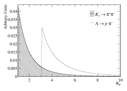
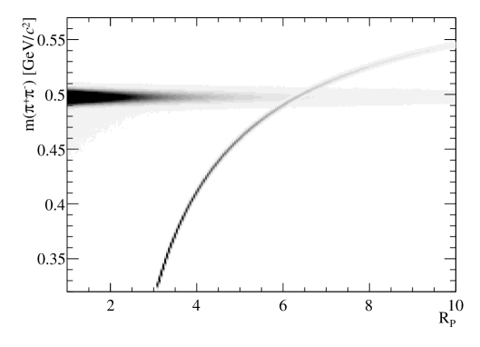
Figure 1: (a) Distribution of the $R_{p}$ variable defined here to be the maximum of $p_{1}/p_{2}$ and $p_{2}/p_{1}$ for the two ${{\mathrm{K}}^{0}_{\mathrm{S}}}\!\rightarrow{{\pi}^{+}}{{\pi}^{-}}$ and ${\Lambda}\!\rightarrow{\mathrm{p}}{{\pi}^{-}}$ simulation samples. b) Invariant mass calculated under the two-pion mass hypothesis for the two simulation samples versus $R_{p}$. Under the $\pi^{+}\pi^{-}$ hypothesis, ${\Lambda}\!\rightarrow{\mathrm{p}}{{\pi}^{-}}$ decays give a characteristic curved band versus $R_{p}$. This illustrates how the two decays can be separated kinematically using the momentum ratio even if particle identification information is unavailable.

Biases on the reconstructed mass arise in several ways and are evaluated by considering the derivatives of equation 3 with respect to $p_{i}$ and $\theta$. One possibility, as detailed in [19] is a bias on the momentum scale, $p_{i}\rightarrow(1+\alpha)p_{i}$. This could arise if the integrated field is mismeasured. If $\alpha$ is the same for both daughters, the observed bias on the parent mass is

$$\Delta m_{P}=\frac{\alpha}{m_{P}}\cdot\>\left(K-m_{1}^{2}\frac{p_{2}}{p_{1}}-m_{2}^{2}\frac{p_{1}}{p_{2}}\right),$$ (4)

where $K=m_{P}^{2}-m_{1}^{2}-m_{2}^{2}$. This can be written as $\Delta{m_{P}}=\alpha\cdot\xi$, where $\xi$ is an effective mass that depends on the masses of the daughter particles and $R_{p}$. If the ${{\mathrm{K}}^{0}_{\mathrm{S}}}\!\rightarrow{{\pi}^{+}}{{\pi}^{-}}$ decay is used to determine $\alpha$ then the correction to the ${\Lambda}$ mass is

$$\Delta m_{{\Lambda}}=\frac{\xi_{{\Lambda}}}{\xi_{{{\mathrm{K}}^{0}_{\mathrm{S}}}}}\cdot\Delta m_{{{\mathrm{K}}^{0}_{\mathrm{S}}}}.$$ (5)

Using the simulation and selection described in Section 3 this evaluates to $\Delta m_{{\Lambda}}\sim 0.15\cdot\Delta m_{{{\mathrm{K}}^{0}_{\mathrm{S}}}}$. This illustrates the power of a ${{\mathrm{K}}^{0}_{\mathrm{S}}}$ calibration sample to control momentum scale uncertainties on the measured ${\Lambda}$ mass. An important subsample for calibration studies is ${{\mathrm{K}}^{0}_{\mathrm{S}}}$ decays with $R_{p}\approx 1$ for which $\Delta m_{{{\mathrm{K}}^{0}_{\mathrm{S}}}}=\alpha\cdot(m_{K}^{2}-4m^{2}_{\pi^{-}})/m_{{{\mathrm{K}}^{0}_{\mathrm{S}}}}$. Noting

$$p^{*}=\frac{\sqrt{m_{{{\mathrm{K}}^{0}_{\mathrm{S}}}}^{2}-4m^{2}_{\pi}}}{2},$$ (6)

equation 4 simplifies to

$$\Delta m_{{{\mathrm{K}}^{0}_{\mathrm{S}}}}=\frac{4\cdot\alpha\cdot p^{*^{2}}}{m_{{{\mathrm{K}}^{0}_{\mathrm{S}}}}}.$$ (7)

A second possibility is a bias from the correction for energy loss in the detector material made in the track fit. In this case, $p_{i}\rightarrow p_{i}+\delta_{i}$. The value of $\delta$ is given by the Bethe equation [3]. It depends on the material traversed and the $\beta\gamma$ of the particle. In the relativistic limit, $\delta$ increases slowly with $p_{i}$ and is reasonably well approximated by

$$\delta_{i}=a_{0}\cdot t\cdot(a_{1}+a_{2}\cdot\textrm{log}(p_{i})),$$ (8)

where $t$ is the thickness of the material and the parameters $a_{i}$ depend on both the material and particle type. The logarithmic dependence on the momentum means that $\delta$ is often taken to be constant, especially at high momentum. The bias on the parent mass from energy loss is

$$\Delta m_{P}=\frac{1}{2\>m_{P}}\cdot\left[\delta_{1}\left(\frac{K-2m_{1}^{2}p_{2}/p_{1}}{p_{1}}\right)+\delta_{2}\left(\frac{K-2m_{2}^{2}p_{1}/p_{2}}{p_{2}}\right)\right],$$ (9)

implying the bias on the mass from the energy loss decreases with increasing daughter momentum. The ${{\mathrm{K}}^{0}_{\mathrm{S}}}\!\rightarrow{{\pi}^{+}}{{\pi}^{-}}$ decay mode is more sensitive to energy-loss than the ${\Lambda}\!\rightarrow{\mathrm{p}}{{\pi}^{-}}$ decay: the ratio of the derivatives is $\sim 0.3$ in this case. The formula simplifies for ${{\mathrm{K}}^{0}_{\mathrm{S}}}$ decays with $R_{p}\approx 1$ where $p_{1}=p_{2}=p_{{{\mathrm{K}}^{0}_{\mathrm{S}}}}/2$ and $\delta=\delta_{1}=\delta_{2}$ to

$$\Delta m_{{{\mathrm{K}}^{0}_{\mathrm{S}}}}=2\cdot\frac{\delta}{p_{{{\mathrm{K}}^{0}_{\mathrm{S}}}}}\cdot\frac{m_{{{\mathrm{K}}^{0}_{\mathrm{S}}}}^{2}-4m^{2}_{\pi^{-}}}{m_{{{\mathrm{K}}^{0}_{\mathrm{S}}}}}=\frac{8p^{*^{2}}\delta}{m_{{{\mathrm{K}}^{0}_{\mathrm{S}}}}\cdot p_{{{\mathrm{K}}^{0}_{\mathrm{S}}}}}.$$ (10)

Another possible effect is a curvature bias due to detector misalignment [20]. For a forward spectrometer, such as LHCb, a misalignment that leads to a curvature bias is a small displacement, in the bending plane, of the detectors upstream and downstream of the magnet. Defining the curvature of the particle $i$ as $\omega_{i}=q_{i}/p_{i}$, where $q_{i}$ is the particle charge, the effect of a curvature bias $\omega_{i}\rightarrow\omega_{i}+\Delta\omega$ on the two-body invariant mass is

$$\Delta m_{P}=\frac{-\Delta\omega}{2\>m_{P}}\cdot\left[q_{1}\cdot p_{1}\left(K-2m_{1}^{2}\frac{p_{2}}{p_{1}}\right)-q_{2}\cdot p_{2}\left(K-2m_{2}^{2}\frac{p_{1}}{p_{2}}\right)\right].$$ (11)

For ${{\mathrm{K}}^{0}_{\mathrm{S}}}\!\rightarrow{{\pi}^{+}}{{\pi}^{-}}$ decays, equation 11 simplifies to $\Delta m_{P}=-\Delta\omega\cdot m_{{{\mathrm{K}}^{0}_{\mathrm{S}}}}\cdot(p_{1}-p_{2})/2$. Since the derivatives with respect to $p_{1}$ and $p_{2}$ have opposite signs, decays with $R_{p}\approx 1$ are unaffected by a curvature bias. In contrast, the reconstructed mass for asymmetric decays is biased, and this bias increases with the magnitude of the difference in the daughter momenta [19]. The change in the sign of the bias for events with $p_{1}>p_{2}$ compared to $p_{2}<p_{1}$ has an interesting consequence. For the ${{\mathrm{K}}^{0}_{\mathrm{S}}}\!\rightarrow{{\pi}^{+}}{{\pi}^{-}}$ decay, where $m_{1}=m_{2}$, if the detector acceptance is the same for particles with positive and negative charge, the average mass of the full sample remains unbiased in the presence of a curvature bias. However, the asymmetry of the decay ${\Lambda}\!\rightarrow{\mathrm{p}}{{\pi}^{-}}$ means that this cancellation occurs only when the decays of ${\Lambda}$ and $\overline{{\Lambda}}$ are considered. Therefore, in CPT tests, care is needed to ensure the absence of a curvature bias. One way to reduce the impact of a curvature bias is to reverse the polarity of the magnetic field, as from equation 11 this gives an additional cancellation. Although a curvature bias will not bias the mean mass value for symmetric decays, it will degrade the resolution, particularly for high-mass states such as the resonances $\Upsilon$ and the $Z^{0}$ boson [19] where the daughter particles have momenta in the range of 0.1-1 TeV. The sensitivity of the $Z^{0}$ sample to this effect is used in [19] to determine the curvature bias using a pseudo-mass method.

The final possibility is that the opening angle between the two particles is biased such that $\theta\rightarrow\theta+\Delta\theta$. This can arise if the daughter particles are not sufficiently separated at the first measurement point to give distinct clusters in the vertex detector. It is straightforward to evaluate the derivative of equation 2 with respect to $\theta$ and determine

$$\Delta m_{P}=\frac{p_{1}p_{2}\cdot\textrm{sin}\theta\cdot\Delta\theta}{m_{P}}.$$ (12)

For a ${{\mathrm{K}}^{0}_{\mathrm{S}}}$ decay with $R\approx 1$ and small $\theta$, equation 3 gives

$$\theta=\frac{2\sqrt{m_{{{\mathrm{K}}^{0}_{\mathrm{S}}}}^{2}-4m_{\pi}^{2}}}{p_{{{\mathrm{K}}^{0}_{\mathrm{S}}}}},$$ (13)

and hence

$$\Delta m_{{{\mathrm{K}}^{0}_{\mathrm{S}}}}\approx\frac{\sqrt{m_{{{\mathrm{K}}^{0}_{\mathrm{S}}}}^{2}-4m_{\pi}^{2}}\cdot p_{{{\mathrm{K}}^{0}_{\mathrm{S}}}}\cdot\Delta\theta}{2m_{{{\mathrm{K}}^{0}_{\mathrm{S}}}}}=\frac{p^{*}\cdot p_{{{\mathrm{K}}^{0}_{\mathrm{S}}}}\cdot\Delta\theta}{m_{{{\mathrm{K}}^{0}_{\mathrm{S}}}}}.$$ (14)

Since the distribution of $cos(\theta)$ is similar for the ${\Lambda}\!\rightarrow{\mathrm{p}}{{\pi}^{-}}$ and ${{\mathrm{K}}^{0}_{\mathrm{S}}}\!\rightarrow{{\pi}^{+}}{{\pi}^{-}}$ decays, the mass bias will be of a comparable magnitude for both modes. Consequently, it is important to correctly determine $\Delta\theta$ in the calibration procedure.

All the biases discussed in this section may be present in the data. For a ${{\mathrm{K}}^{0}_{\mathrm{S}}}$ decay with $R_{p}\approx 1$ the total bias is given by

$$\Delta m_{{{\mathrm{K}}^{0}_{\mathrm{S}}}}=\frac{4p^{*^{2}}}{m_{{{\mathrm{K}}^{0}_{\mathrm{S}}}}}\cdot\left(\alpha+\frac{2\delta}{p_{{{\mathrm{K}}^{0}_{\mathrm{S}}}}}+\frac{p_{{{\mathrm{K}}^{0}_{\mathrm{S}}}}}{4p^{*}}\Delta\theta\right).$$ (15)

Although this equation has been derived for the ${{\mathrm{K}}^{0}_{\mathrm{S}}}\!\rightarrow{{\pi}^{+}}{{\pi}^{-}}$ decay, it applies to any symmetric two-body decay to daughter particles with equal mass. For calibration, a fit of equation 15 to $\Delta m_{{{\mathrm{K}}^{0}_{\mathrm{S}}}}$ in subsamples of $p_{{{\mathrm{K}}^{0}_{\mathrm{S}}}}$ for symmetric ${{\mathrm{K}}^{0}_{\mathrm{S}}}$ decays determines the parameters $\alpha,\delta$ and $\Delta\theta$. In a second step, the presence of a curvature bias can be quantified by fitting the mass in subsamples of the momentum difference for the full sample of ${{\mathrm{K}}^{0}_{\mathrm{S}}}\!\rightarrow{{\pi}^{+}}{{\pi}^{-}}$ decays.

5 Quantifying and correcting biases: determining the ${\Lambda}$ mass

The accuracy of the calibration procedure proposed in Section 4 is studied using the simulation described in Section 3 for the example of the LHCb detector. Two illustrative studies are performed to validate the method using publicly available information on detector performance. For these studies, reasonable ranges for the parameters $\alpha$, $\delta$, $\Delta\theta$ and $\Delta\omega$ are chosen based on available LHCb performance information (table 1). Reference [18] states that the LHCb detector material is known with a relative precision of $10\%$. From [21] a particle sees on average a $35\,\%$ of a radiation length ($X_{0}$) of material before the LHCb dipole magnet. Multiplying these values gives $\Delta X_{0}=t/X_{0}^{\textrm{Si}}=3.5\,\%$ listed in table 1. To convert from $X_{0}^{Si}$ to $\delta$ the detector material is taken to be silicon and the expected energy loss is generated using the Bethe formula using the information on material properties in  [3, 22]. In the calibration procedure, equation 8 is used. To fit the ${{\mathrm{K}}^{0}_{\mathrm{S}}}$ and ${\Lambda}$ invariant-mass distributions, a Crystal Ball function is used [23]. In this way, the impact of radiative corrections is taken into account following the procedure described in [19]. In these illustrative studies, the influence of background is ignored. The relatively long lifetime of the ${{\mathrm{K}}^{0}_{\mathrm{S}}}$ means that the combinatorial background is small. In a more realistic study, the background of ${\Lambda}\!\rightarrow{\mathrm{p}}{{\pi}^{-}}$ decays should be considered. Figure 1(b) shows that background from this source does not have an impact when selecting candidates with $R_{p}\approx 1$. However, ${\Lambda}\!\rightarrow{\mathrm{p}}{{\pi}^{-}}$ decays must be vetoed or included as a component in fits to the full sample.

Table 1: Ranges considered on the calibration parameters. In pseudoexperiments each parameter is sampled from a Gaussian distribution with mean zero and $\sigma$ given in this table. In the absence of available information, a reasonable range for $\Delta\theta$ is chosen.

• Parameter	$\sigma$	Source
  $\alpha$	$3\times 10^{-4}$	Accuracy reported in [19]
  $\Delta X_{0}$	$3.5\,\%$	Information from [18, 21]
  $\Delta\theta$	$5\times 10^{-6}\,\textrm{rad}$	—
  $\Delta\omega$	$5\times 10^{-5}\,\textrm{c/GeV}$	Accuracy reported in [24]

In the first study, it is assumed that curvature biases are negligible ($\Delta\omega=0$) because they are determined from studies of the $Z^{0}$ boson or reduced by reversing the polarity of the dipole magnet. One hundred pseudoexperiments are generated, each with a random set of values of $\alpha,\delta$, and $\Delta\theta$ generated using the values in table 1.

For calibration, symmetric ${{\mathrm{K}}^{0}_{\mathrm{S}}}\!\rightarrow{{\pi}^{+}}{{\pi}^{-}}$ decays with $0.91<R_{p}<1.1$ are selected. This corresponds to $\sim 10\,\%$ of the events in the ${{\mathrm{K}}^{0}_{\mathrm{S}}}$ sample and is large enough to determine with high precision without introducing large biases from the assumptions made in equation 15. The window on $R_{p}$ is chosen to be slightly asymmetric so that the average value of the sample is one. Fitting the ${{\mathrm{K}}^{0}_{\mathrm{S}}}$ and ${\Lambda}$ invariant mass distributions for these pseudoexperiments gives the distributions in figure 2 for the mass bias. As expected, the RMS of the distribution for the ${\Lambda}$ mass is a factor of 4-5 less than for the ${{\mathrm{K}}^{0}_{\mathrm{S}}}$ case.

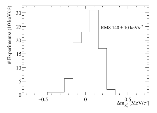
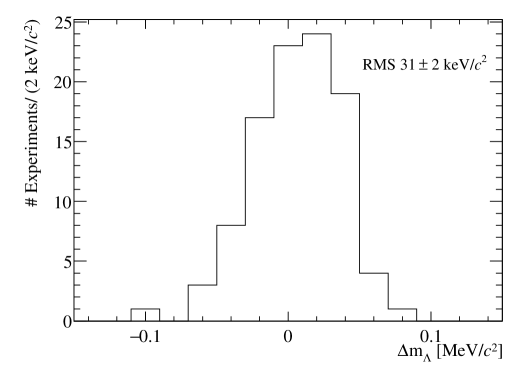
Figure 2: (a) Distribution of $\Delta m_{{{\mathrm{K}}^{0}_{\mathrm{S}}}}$ in pseudoexperiments determined from a fit of a Crystal Ball function to the full sample. (b) Distribution of $\Delta M({\Lambda})$ in pseudoexperiments from a Crystal Ball function fit. Note the change in scale on the $x-$axis.

To determine the calibration parameters $\alpha,X_{0}$ and $\Delta\theta$, the symmetric ${{\mathrm{K}}^{0}_{\mathrm{S}}}$ data set is divided into ten subsamples of $\mathrm{K}$ each with an equal number of entries. A fit of a Crystal Ball function is made to each subsample. Fitting equation 15 to the resulting $\Delta m_{{{\mathrm{K}}^{0}_{\mathrm{S}}}}$ values determines the calibration parameters. In a second step, the overall scale is fixed to $m_{{{\mathrm{K}}^{0}_{\mathrm{S}}}}$ by fitting the full sample with no requirement on $R_{p}$. Figure 3 shows $\Delta m_{{{\mathrm{K}}^{0}_{\mathrm{S}}}}$ versus $p_{{{\mathrm{K}}^{0}_{\mathrm{S}}}}$ for an example pseudoexperiment before and after the calibration procedure. The model given by equation 15 describes the simulated data well. Table 2 summarizes the bias and spread of the calibration parameters and masses. Although there are small biases on the fitted parameters, the bias on the ${\Lambda}$ mass calculated using the parameters is $0.1\,\textrm{keV}$ with a standard deviation of $0.2\,\textrm{keV}/c^{2}$. These should be compared to the statistical uncertainty on $m({\Lambda})$ of $0.6\,\textrm{keV}/c^{2}$ and the $2\,\textrm{keV}/c^{2}$ uncertainty from the knowledge of $m_{{{\mathrm{K}}^{0}_{\mathrm{S}}}}$.

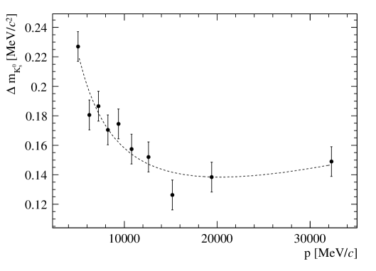
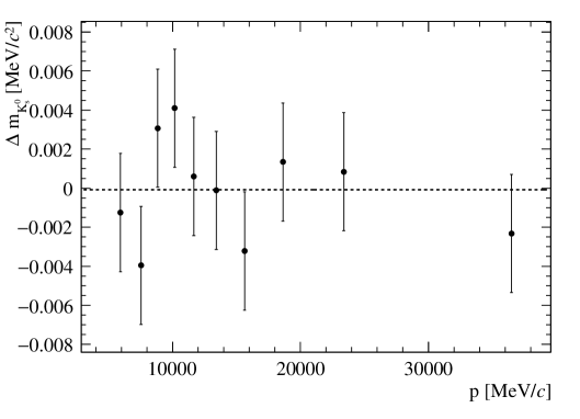
Figure 3: Distribution of $\Delta m_{{{\mathrm{K}}^{0}_{\mathrm{S}}}}$ in an example pseudoexperiment with $\alpha=1.5\times 10^{-4},\delta=2.6\,\textrm{MeV}$ and $\Delta\theta=5\times 10^{-6}\,\textrm{rad}$. (a) Before calibration. A fit to equation 15 is superimposed (b) After calibration. A fit to a constant is superimposed. The probability of $\chi^{2}$ of the fit is 0.66. Note the change of scale on the $y-$axis.

Table 2: Bias and uncertainty (standard deviation) on the fitted calibration parameters.

• Parameter	Bias	Uncertainty
  $\alpha$	$-(1.32\pm 0.03)\times 10^{-5}$	$3\times 10^{-7}$
  $X_{0}$	$(-0.46\pm 0.07)\times 10^{-3}$	$0.7\times 10^{-3}$
  $\Delta\theta$ [mrad]	$(4.6\pm 0.1)\times 10^{-7}$	$1.3\times 10^{-7}$

In the second, more extended study, the impact of a curvature bias is also studied. The primary step of the calibration procedure to determine $\alpha,X_{0}$ and $\Delta\theta$ is the same as in the first study described above. To determine $\Delta\omega$, the mass is recalculated with the values obtained for these parameters and the fits are made in subsamples of the momentum difference. A linear fit of the resulting values of $\Delta m_{{{\mathrm{K}}^{0}_{\mathrm{S}}}}$ determines $\Delta\omega$ (from the slope) and the global scale of the full sample (from the offset). This procedure is iterated once.

Figure 4 shows $\Delta m_{{{\mathrm{K}}^{0}_{\mathrm{S}}}}$ versus the momentum difference of the daughters after the primary calibration and the extended calibration procedure. After calibration, the bias on the mass is consistent with being flat versus the mass difference. The bias obtained across the 100 pseudoexperiments is similar to the first study ($0.2\,\textrm{keV}/c^{2}$) but the uncertainty determined from the standard deviation across the pseudoexperiments increases to $0.7\,\textrm{keV}/c^{2}$. Before calibration, the standard deviation of $m({\Lambda})-m(\overline{{\Lambda}})$ is $30\,\textrm{keV}/c^{2}$, which highlights the importance of correcting curvature biases for the $CPT$ tests. After calibration, the standard deviation reduces to $1.3\,\textrm{keV}/c^{2}$ and there is a bias of $0.6\,\textrm{keV}/c^{2}$. This study indicates that it is possible to probe $R_{CPT}$ to the $10^{-6}$ level at LHCb. This would be an order of magnitude improvement compared to current knowledge. Better control of the systematic uncertainty from the knowledge of $\Delta\omega$ can be achieved by using a $Z^{0}$ boson sample as in [24], reversal of the magnetic field and selecting regions of phase space where the detector acceptance is equal for particles of opposite charge.

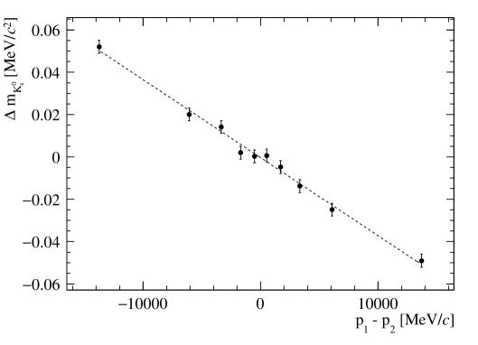
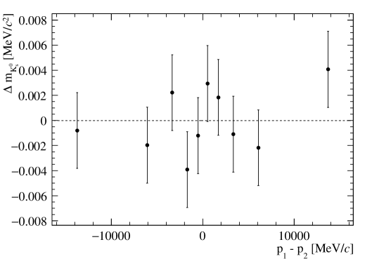
Figure 4: Distribution of $\Delta m_{{{\mathrm{K}}^{0}_{\mathrm{S}}}}$ in an example pseudoexperiment with $\alpha=1.5\times 10^{-4},\delta=2.6\,\textrm{MeV}$, $\Delta\theta=5\times 10^{-6}\,\textrm{rad}$ and $\Delta\omega=-1.5\times 10^{-5}\textrm{c/GeV}$. (a) After the primary calibration step. A fit to linear form is superimposed (b) After the full calibration. A fit to a constant is superimposed. The probability of $\chi^{2}$ of the fit is 0.66. Note the change of scale on the $y-$axis.

In addition to the effects discussed in this paper, other biases need to be considered in a realistic study. Decays-in-flight and hadronic interactions in the detector give asymmetric tails in the resolution function. As described in [25], these can be rejected using muon detector and track quality information. A particular challenge for measurements at the LHC is the high-multiplicity environment, which means that hits from other particles might be wrongly assigned to the reconstructed trajectory close to the decay-vertex leading to a biased opening angle measurement.

Physics at the LHC is focused on short-lived particles with decay vertices close to the interaction point. Consequently, the track reconstruction may make assumptions that lead to biases for longer-lived particles necessitating a calibration as a function of the decay-vertex position. Biases of this type are discussed in the context of the ALICE experiment in [26] and would need to be quantified in a realistic study.

Finally, during the LHCb track reconstruction, particle identification information is not available. Hence, the applied energy-loss correction assumes that all particles are pions [19]. The impact of this assumption for the case of the LHCb detector is evaluated using the simulation described above. Assuming $35\,\%\,X_{0}$ of silicon before the dipole magnet, the bias on the reconstructed proton momentum is $\sim 2$ MeV$/c$, largely independent of the proton momentum. This momentum bias causes the reconstructed ${\Lambda}$ mass to be shifted by $0.006\,\mathrm{MeV}/c^{2}$. Given the size of this effect, it needs to be taken into account.

6 Conclusions

In this paper a general formalism to quantify and correct biases on the invariant mass for two-body decays has been developed. It has been emphasised that insights into detector performance can be achieved by relating observed biases to physical detector parameters.

To illustrate the method, the example of measuring the ${\Lambda}$ mass at LHCb has been considered. Even with a modest sample of around $4\times 10^{7}$ candidates, the statistical precision can be improved by an order of magnitude compared to previous studies. Currently, the dominant systematic uncertainty is due to the knowledge of $m_{{{\mathrm{K}}^{0}_{\mathrm{S}}}}$. The simplified studies here indicate that systematic uncertainties can be controlled in a detector such as LHCb to the required level. The framework developed also allows to probe for unaccounted for effects. In addition to improving the knowledge of the ${\Lambda}$ mass itself, comparison of the measured ${\Lambda}$ and $\overline{{\Lambda}}$ mass gives a $CPT$ test with at least an order of magnitude improvement in precision assuming curvature biases are kept under control. Although there are certainly challenges beyond those studied here, this appears to be an interesting avenue for further study.

References

References

- [1] Fodor Z and Hoelbling C 2012 Rev. Mod. Phys. 84 449
- [2] Sozzi M S 2008 Discrete symmetries and CP violation Oxford graduate texts (New York, NY: Oxford Univ. Press) URL https://cds.cern.ch/record/1087897
- [3] Navas S et al. (Particle Data Group) 2024 Phys. Rev. D110 030001
- [4] Hartouni E et al. 1994 Phys. Rev. Lett. 72 1322–1325
- [5] Bhowmik B and Goyal D P 1963 Nuovo Cim. 28 1494
- [6] Schmidt P 1965 Phys. Rev. 140 B1328
- [7] London G et al. 1966 Phys. Rev. 143 1034–1091
- [8] Mayeur C, E Tompa E and Wickens J 1967 Univ. Brux., Inst. Phys., Bull. No. 32, 1-5(Jan. 1967).
- [9] Hyman L et al. 1972 Phys. Rev. D 5 1063–1068
- [10] Alves Jr A A et al. (LHCb collaboration) 2008 JINST 3 S08005
- [11] Cowan G, Craik D and Needham M 2017 Comput. Phys. Commun. 214 239–246
- [12] Lange D J 2001 Nucl. Instrum. Meth. A462 152–155
- [13] Golonka P and Was Z 2006 Eur. Phys. J. C45 97–107
- [14] Acharya S et al. (ALICE) 2021 Eur. Phys. J. C 81 256
- [15] Maguire E, Lukas H and Watt G 2017 J. Phys. Conf. Ser. 898 102006
- [16] Aaij R et al. (LHCb) 2011 JHEP 08 034 (Preprint 1107.0882)
- [17] Aaij R et al. (LHCb) 2013 JHEP 01 090 (Preprint 1209.4029)
- [18] Aaij R et al. (LHCb) 2015 Int. J. Mod. Phys. A 30 1530022 (Preprint 1412.6352)
- [19] Aaij R et al. (LHCb) 2024 JINST 19 P02008
- [20] Amoraal J et al. 2013 Nucl. Instrum. Meth. A712 48–55 (Preprint 1207.4756)
- [21] Fave V 2008 CERN-LHCB-2008-054
- [22] Sternheimer R M, Berger M J and Seltzer S M 1984 Atom. Data Nucl. Data Tabl. 30 261–271
- [23] Skwarnicki T 1986 A study of the radiative cascade transitions between the Upsilon-prime and Upsilon resonances Ph.D. thesis Institute of Nuclear Physics, Krakow DESY-F31-86-02
- [24] Aaij R et al. (LHCb) 2024 JINST 19 P03010 (Preprint 2311.04670)
- [25] Aaij R et al. (LHCb) 2025 (Preprint 2507.20945)
- [26] Skorodumovs G 2020 Test of CPT theorem invariance via mass difference of baryons Master’s thesis University of Heidelberg