EUROPEAN ORGANIZATION FOR NUCLEAR RESEARCH (CERN)

​​​ CERN-PH-EP-2012-267 LHCb-PAPER-2012-023 18 September 2012

Search for the rare decay $K_{\rm\scriptscriptstyle S}^{0}\rightarrow\mu^{+}\mu^{-}$

The LHCb collaboration

A search for the decay $K_{\rm\scriptscriptstyle S}^{0}\rightarrow\mu^{+}\mu^{-}$ is performed, based on a data sample of 1.0 fb^-1 of $pp$ collisions at $\sqrt{s}$ = 7 TeV collected by the LHCb experiment at the Large Hadron Collider. The observed number of candidates is consistent with the background-only hypothesis, yielding an upper limit of $\mathcal{B}(K_{\rm\scriptscriptstyle S}^{0}\rightarrow\mu^{+}\mu^{-})<11(9)\times 10^{-9}$ at 95 (90)$\%$ confidence level. This limit is a factor of thirty below the previous measurement.

Published in the Journal of High Energy Physics

 

LHCb collaboration

R. Aaij³⁸, C. Abellan Beteta^33,n, A. Adametz¹¹, B. Adeva³⁴, M. Adinolfi⁴³, C. Adrover⁶, A. Affolder⁴⁹, Z. Ajaltouni⁵, J. Albrecht³⁵, F. Alessio³⁵, M. Alexander⁴⁸, S. Ali³⁸, G. Alkhazov²⁷, P. Alvarez Cartelle³⁴, A.A. Alves Jr²², S. Amato², Y. Amhis³⁶, L. Anderlini^17,f, J. Anderson³⁷, R.B. Appleby⁵¹, O. Aquines Gutierrez¹⁰, F. Archilli^18,35, A. Artamonov ³², M. Artuso⁵³, E. Aslanides⁶, G. Auriemma^22,m, S. Bachmann¹¹, J.J. Back⁴⁵, C. Baesso⁵⁴, W. Baldini¹⁶, R.J. Barlow⁵¹, C. Barschel³⁵, S. Barsuk⁷, W. Barter⁴⁴, A. Bates⁴⁸, Th. Bauer³⁸, A. Bay³⁶, J. Beddow⁴⁸, I. Bediaga¹, S. Belogurov²⁸, K. Belous³², I. Belyaev²⁸, E. Ben-Haim⁸, M. Benayoun⁸, G. Bencivenni¹⁸, S. Benson⁴⁷, J. Benton⁴³, A. Berezhnoy²⁹, R. Bernet³⁷, M.-O. Bettler⁴⁴, M. van Beuzekom³⁸, A. Bien¹¹, S. Bifani¹², T. Bird⁵¹, A. Bizzeti^17,h, P.M. Bjørnstad⁵¹, T. Blake³⁵, F. Blanc³⁶, C. Blanks⁵⁰, J. Blouw¹¹, S. Blusk⁵³, A. Bobrov³¹, V. Bocci²², A. Bondar³¹, N. Bondar²⁷, W. Bonivento¹⁵, S. Borghi^48,51, A. Borgia⁵³, T.J.V. Bowcock⁴⁹, C. Bozzi¹⁶, T. Brambach⁹, J. van den Brand³⁹, J. Bressieux³⁶, D. Brett⁵¹, M. Britsch¹⁰, T. Britton⁵³, N.H. Brook⁴³, H. Brown⁴⁹, A. Büchler-Germann³⁷, I. Burducea²⁶, A. Bursche³⁷, J. Buytaert³⁵, S. Cadeddu¹⁵, O. Callot⁷, M. Calvi^20,j, M. Calvo Gomez^33,n, A. Camboni³³, P. Campana^18,35, A. Carbone^14,c, G. Carboni^21,k, R. Cardinale^19,i, A. Cardini¹⁵, L. Carson⁵⁰, K. Carvalho Akiba², G. Casse⁴⁹, M. Cattaneo³⁵, Ch. Cauet⁹, M. Charles⁵², Ph. Charpentier³⁵, P. Chen^3,36, N. Chiapolini³⁷, M. Chrzaszcz ²³, K. Ciba³⁵, X. Cid Vidal³⁴, G. Ciezarek⁵⁰, P.E.L. Clarke⁴⁷, M. Clemencic³⁵, H.V. Cliff⁴⁴, J. Closier³⁵, C. Coca²⁶, V. Coco³⁸, J. Cogan⁶, E. Cogneras⁵, P. Collins³⁵, A. Comerma-Montells³³, A. Contu^52,15, A. Cook⁴³, M. Coombes⁴³, G. Corti³⁵, B. Couturier³⁵, G.A. Cowan³⁶, D. Craik⁴⁵, S. Cunliffe⁵⁰, R. Currie⁴⁷, C. D’Ambrosio³⁵, P. David⁸, P.N.Y. David³⁸, I. De Bonis⁴, K. De Bruyn³⁸, S. De Capua^21,k, M. De Cian³⁷, J.M. De Miranda¹, L. De Paula², P. De Simone¹⁸, D. Decamp⁴, M. Deckenhoff⁹, H. Degaudenzi^36,35, L. Del Buono⁸, C. Deplano¹⁵, D. Derkach¹⁴, O. Deschamps⁵, F. Dettori³⁹, A. Di Canto¹¹, J. Dickens⁴⁴, H. Dijkstra³⁵, P. Diniz Batista¹, F. Domingo Bonal^33,n, S. Donleavy⁴⁹, F. Dordei¹¹, A. Dosil Suárez³⁴, D. Dossett⁴⁵, A. Dovbnya⁴⁰, F. Dupertuis³⁶, R. Dzhelyadin³², A. Dziurda²³, A. Dzyuba²⁷, S. Easo⁴⁶, U. Egede⁵⁰, V. Egorychev²⁸, S. Eidelman³¹, D. van Eijk³⁸, S. Eisenhardt⁴⁷, R. Ekelhof⁹, L. Eklund⁴⁸, I. El Rifai⁵, Ch. Elsasser³⁷, D. Elsby⁴², D. Esperante Pereira³⁴, A. Falabella^14,e, C. Färber¹¹, G. Fardell⁴⁷, C. Farinelli³⁸, S. Farry¹², V. Fave³⁶, V. Fernandez Albor³⁴, F. Ferreira Rodrigues¹, M. Ferro-Luzzi³⁵, S. Filippov³⁰, C. Fitzpatrick³⁵, M. Fontana¹⁰, F. Fontanelli^19,i, R. Forty³⁵, O. Francisco², M. Frank³⁵, C. Frei³⁵, M. Frosini^17,f, S. Furcas²⁰, A. Gallas Torreira³⁴, D. Galli^14,c, M. Gandelman², P. Gandini⁵², Y. Gao³, J-C. Garnier³⁵, J. Garofoli⁵³, J. Garra Tico⁴⁴, L. Garrido³³, C. Gaspar³⁵, R. Gauld⁵², E. Gersabeck¹¹, M. Gersabeck³⁵, T. Gershon^45,35, Ph. Ghez⁴, V. Gibson⁴⁴, V.V. Gligorov³⁵, C. Göbel⁵⁴, D. Golubkov²⁸, A. Golutvin^50,28,35, A. Gomes², H. Gordon⁵², M. Grabalosa Gándara³³, R. Graciani Diaz³³, L.A. Granado Cardoso³⁵, E. Graugés³³, G. Graziani¹⁷, A. Grecu²⁶, E. Greening⁵², S. Gregson⁴⁴, O. Grünberg⁵⁵, B. Gui⁵³, E. Gushchin³⁰, Yu. Guz³², T. Gys³⁵, C. Hadjivasiliou⁵³, G. Haefeli³⁶, C. Haen³⁵, S.C. Haines⁴⁴, S. Hall⁵⁰, T. Hampson⁴³, S. Hansmann-Menzemer¹¹, N. Harnew⁵², S.T. Harnew⁴³, J. Harrison⁵¹, P.F. Harrison⁴⁵, T. Hartmann⁵⁵, J. He⁷, V. Heijne³⁸, K. Hennessy⁴⁹, P. Henrard⁵, J.A. Hernando Morata³⁴, E. van Herwijnen³⁵, E. Hicks⁴⁹, D. Hill⁵², M. Hoballah⁵, P. Hopchev⁴, W. Hulsbergen³⁸, P. Hunt⁵², T. Huse⁴⁹, N. Hussain⁵², R.S. Huston¹², D. Hutchcroft⁴⁹, D. Hynds⁴⁸, V. Iakovenko⁴¹, P. Ilten¹², J. Imong⁴³, R. Jacobsson³⁵, A. Jaeger¹¹, M. Jahjah Hussein⁵, E. Jans³⁸, F. Jansen³⁸, P. Jaton³⁶, B. Jean-Marie⁷, F. Jing³, M. John⁵², D. Johnson⁵², C.R. Jones⁴⁴, B. Jost³⁵, M. Kaballo⁹, S. Kandybei⁴⁰, M. Karacson³⁵, T.M. Karbach⁹, J. Keaveney¹², I.R. Kenyon⁴², U. Kerzel³⁵, T. Ketel³⁹, A. Keune³⁶, B. Khanji²⁰, Y.M. Kim⁴⁷, O. Kochebina⁷, V. Komarov^36,29, R.F. Koopman³⁹, P. Koppenburg³⁸, M. Korolev²⁹, A. Kozlinskiy³⁸, L. Kravchuk³⁰, K. Kreplin¹¹, M. Kreps⁴⁵, G. Krocker¹¹, P. Krokovny³¹, F. Kruse⁹, M. Kucharczyk^20,23,j, V. Kudryavtsev³¹, T. Kvaratskheliya^28,35, V.N. La Thi³⁶, D. Lacarrere³⁵, G. Lafferty⁵¹, A. Lai¹⁵, D. Lambert⁴⁷, R.W. Lambert³⁹, E. Lanciotti³⁵, G. Lanfranchi^18,35, C. Langenbruch³⁵, T. Latham⁴⁵, C. Lazzeroni⁴², R. Le Gac⁶, J. van Leerdam³⁸, J.-P. Lees⁴, R. Lefèvre⁵, A. Leflat^29,35, J. Lefrançois⁷, O. Leroy⁶, T. Lesiak²³, Y. Li³, L. Li Gioi⁵, M. Liles⁴⁹, R. Lindner³⁵, C. Linn¹¹, B. Liu³, G. Liu³⁵, J. von Loeben²⁰, J.H. Lopes², E. Lopez Asamar³³, N. Lopez-March³⁶, H. Lu³, J. Luisier³⁶, A. Mac Raighne⁴⁸, F. Machefert⁷, I.V. Machikhiliyan^4,28, F. Maciuc²⁶, O. Maev^27,35, J. Magnin¹, M. Maino²⁰, S. Malde⁵², G. Manca^15,d, G. Mancinelli⁶, N. Mangiafave⁴⁴, U. Marconi¹⁴, R. Märki³⁶, J. Marks¹¹, G. Martellotti²², A. Martens⁸, L. Martin⁵², A. Martín Sánchez⁷, M. Martinelli³⁸, D. Martinez Santos³⁵, A. Massafferri¹, Z. Mathe³⁵, C. Matteuzzi²⁰, M. Matveev²⁷, E. Maurice⁶, A. Mazurov^16,30,35, J. McCarthy⁴², G. McGregor⁵¹, R. McNulty¹², M. Meissner¹¹, M. Merk³⁸, J. Merkel⁹, D.A. Milanes¹³, M.-N. Minard⁴, J. Molina Rodriguez⁵⁴, S. Monteil⁵, D. Moran⁵¹, P. Morawski²³, R. Mountain⁵³, I. Mous³⁸, F. Muheim⁴⁷, K. Müller³⁷, R. Muresan²⁶, B. Muryn²⁴, B. Muster³⁶, J. Mylroie-Smith⁴⁹, P. Naik⁴³, T. Nakada³⁶, R. Nandakumar⁴⁶, I. Nasteva¹, M. Needham⁴⁷, N. Neufeld³⁵, A.D. Nguyen³⁶, C. Nguyen-Mau^36,o, M. Nicol⁷, V. Niess⁵, N. Nikitin²⁹, T. Nikodem¹¹, A. Nomerotski^52,35, A. Novoselov³², A. Oblakowska-Mucha²⁴, V. Obraztsov³², S. Oggero³⁸, S. Ogilvy⁴⁸, O. Okhrimenko⁴¹, R. Oldeman^15,d,35, M. Orlandea²⁶, J.M. Otalora Goicochea², P. Owen⁵⁰, B.K. Pal⁵³, A. Palano^13,b, M. Palutan¹⁸, J. Panman³⁵, A. Papanestis⁴⁶, M. Pappagallo⁴⁸, C. Parkes⁵¹, C.J. Parkinson⁵⁰, G. Passaleva¹⁷, G.D. Patel⁴⁹, M. Patel⁵⁰, G.N. Patrick⁴⁶, C. Patrignani^19,i, C. Pavel-Nicorescu²⁶, A. Pazos Alvarez³⁴, A. Pellegrino³⁸, G. Penso^22,l, M. Pepe Altarelli³⁵, S. Perazzini^14,c, D.L. Perego^20,j, E. Perez Trigo³⁴, A. Pérez-Calero Yzquierdo³³, P. Perret⁵, M. Perrin-Terrin⁶, G. Pessina²⁰, K. Petridis⁵⁰, A. Petrolini^19,i, A. Phan⁵³, E. Picatoste Olloqui³³, B. Pie Valls³³, B. Pietrzyk⁴, T. Pilař⁴⁵, D. Pinci²², S. Playfer⁴⁷, M. Plo Casasus³⁴, F. Polci⁸, G. Polok²³, A. Poluektov^45,31, E. Polycarpo², D. Popov¹⁰, B. Popovici²⁶, C. Potterat³³, A. Powell⁵², J. Prisciandaro³⁶, V. Pugatch⁴¹, A. Puig Navarro³⁶, W. Qian³, J.H. Rademacker⁴³, B. Rakotomiaramanana³⁶, M.S. Rangel², I. Raniuk⁴⁰, N. Rauschmayr³⁵, G. Raven³⁹, S. Redford⁵², M.M. Reid⁴⁵, A.C. dos Reis¹, S. Ricciardi⁴⁶, A. Richards⁵⁰, K. Rinnert⁴⁹, V. Rives Molina³³, D.A. Roa Romero⁵, P. Robbe⁷, E. Rodrigues^48,51, P. Rodriguez Perez³⁴, G.J. Rogers⁴⁴, S. Roiser³⁵, V. Romanovsky³², A. Romero Vidal³⁴, J. Rouvinet³⁶, T. Ruf³⁵, H. Ruiz³³, G. Sabatino^21,k, J.J. Saborido Silva³⁴, N. Sagidova²⁷, P. Sail⁴⁸, B. Saitta^15,d, C. Salzmann³⁷, B. Sanmartin Sedes³⁴, M. Sannino^19,i, R. Santacesaria²², C. Santamarina Rios³⁴, R. Santinelli³⁵, E. Santovetti^21,k, M. Sapunov⁶, A. Sarti^18,l, C. Satriano^22,m, A. Satta²¹, M. Savrie^16,e, P. Schaack⁵⁰, M. Schiller³⁹, H. Schindler³⁵, S. Schleich⁹, M. Schlupp⁹, M. Schmelling¹⁰, B. Schmidt³⁵, O. Schneider³⁶, A. Schopper³⁵, M.-H. Schune⁷, R. Schwemmer³⁵, B. Sciascia¹⁸, A. Sciubba^18,l, M. Seco³⁴, A. Semennikov²⁸, K. Senderowska²⁴, I. Sepp⁵⁰, N. Serra³⁷, J. Serrano⁶, P. Seyfert¹¹, M. Shapkin³², I. Shapoval^40,35, P. Shatalov²⁸, Y. Shcheglov²⁷, T. Shears^49,35, L. Shekhtman³¹, O. Shevchenko⁴⁰, V. Shevchenko²⁸, A. Shires⁵⁰, R. Silva Coutinho⁴⁵, T. Skwarnicki⁵³, N.A. Smith⁴⁹, E. Smith^52,46, M. Smith⁵¹, K. Sobczak⁵, F.J.P. Soler⁴⁸, A. Solomin⁴³, F. Soomro^18,35, D. Souza⁴³, B. Souza De Paula², B. Spaan⁹, A. Sparkes⁴⁷, P. Spradlin⁴⁸, F. Stagni³⁵, S. Stahl¹¹, O. Steinkamp³⁷, S. Stoica²⁶, S. Stone⁵³, B. Storaci³⁸, M. Straticiuc²⁶, U. Straumann³⁷, V.K. Subbiah³⁵, S. Swientek⁹, M. Szczekowski²⁵, P. Szczypka^36,35, T. Szumlak²⁴, S. T’Jampens⁴, M. Teklishyn⁷, E. Teodorescu²⁶, F. Teubert³⁵, C. Thomas⁵², E. Thomas³⁵, J. van Tilburg¹¹, V. Tisserand⁴, M. Tobin³⁷, S. Tolk³⁹, S. Topp-Joergensen⁵², N. Torr⁵², E. Tournefier^4,50, S. Tourneur³⁶, M.T. Tran³⁶, A. Tsaregorodtsev⁶, N. Tuning³⁸, M. Ubeda Garcia³⁵, A. Ukleja²⁵, D. Urner⁵¹, U. Uwer¹¹, V. Vagnoni¹⁴, G. Valenti¹⁴, R. Vazquez Gomez³³, P. Vazquez Regueiro³⁴, S. Vecchi¹⁶, J.J. Velthuis⁴³, M. Veltri^17,g, G. Veneziano³⁶, M. Vesterinen³⁵, B. Viaud⁷, I. Videau⁷, D. Vieira², X. Vilasis-Cardona^33,n, J. Visniakov³⁴, A. Vollhardt³⁷, D. Volyanskyy¹⁰, D. Voong⁴³, A. Vorobyev²⁷, V. Vorobyev³¹, H. Voss¹⁰, C. Voß⁵⁵, R. Waldi⁵⁵, R. Wallace¹², S. Wandernoth¹¹, J. Wang⁵³, D.R. Ward⁴⁴, N.K. Watson⁴², A.D. Webber⁵¹, D. Websdale⁵⁰, M. Whitehead⁴⁵, J. Wicht³⁵, D. Wiedner¹¹, L. Wiggers³⁸, G. Wilkinson⁵², M.P. Williams^45,46, M. Williams^50,p, F.F. Wilson⁴⁶, J. Wishahi⁹, M. Witek^23,35, W. Witzeling³⁵, S.A. Wotton⁴⁴, S. Wright⁴⁴, S. Wu³, K. Wyllie³⁵, Y. Xie⁴⁷, F. Xing⁵², Z. Xing⁵³, Z. Yang³, R. Young⁴⁷, X. Yuan³, O. Yushchenko³², M. Zangoli¹⁴, M. Zavertyaev^10,a, F. Zhang³, L. Zhang⁵³, W.C. Zhang¹², Y. Zhang³, A. Zhelezov¹¹, L. Zhong³, A. Zvyagin³⁵.

¹Centro Brasileiro de Pesquisas Físicas (CBPF), Rio de Janeiro, Brazil
²Universidade Federal do Rio de Janeiro (UFRJ), Rio de Janeiro, Brazil
³Center for High Energy Physics, Tsinghua University, Beijing, China
⁴LAPP, Université de Savoie, CNRS/IN2P3, Annecy-Le-Vieux, France
⁵Clermont Université, Université Blaise Pascal, CNRS/IN2P3, LPC, Clermont-Ferrand, France
⁶CPPM, Aix-Marseille Université, CNRS/IN2P3, Marseille, France
⁷LAL, Université Paris-Sud, CNRS/IN2P3, Orsay, France
⁸LPNHE, Université Pierre et Marie Curie, Université Paris Diderot, CNRS/IN2P3, Paris, France
⁹Fakultät Physik, Technische Universität Dortmund, Dortmund, Germany
¹⁰Max-Planck-Institut für Kernphysik (MPIK), Heidelberg, Germany
¹¹Physikalisches Institut, Ruprecht-Karls-Universität Heidelberg, Heidelberg, Germany
¹²School of Physics, University College Dublin, Dublin, Ireland
¹³Sezione INFN di Bari, Bari, Italy
¹⁴Sezione INFN di Bologna, Bologna, Italy
¹⁵Sezione INFN di Cagliari, Cagliari, Italy
¹⁶Sezione INFN di Ferrara, Ferrara, Italy
¹⁷Sezione INFN di Firenze, Firenze, Italy
¹⁸Laboratori Nazionali dell’INFN di Frascati, Frascati, Italy
¹⁹Sezione INFN di Genova, Genova, Italy
²⁰Sezione INFN di Milano Bicocca, Milano, Italy
²¹Sezione INFN di Roma Tor Vergata, Roma, Italy
²²Sezione INFN di Roma La Sapienza, Roma, Italy
²³Henryk Niewodniczanski Institute of Nuclear Physics Polish Academy of Sciences, Kraków, Poland
²⁴AGH University of Science and Technology, Kraków, Poland
²⁵National Center for Nuclear Research (NCBJ), Warsaw, Poland
²⁶Horia Hulubei National Institute of Physics and Nuclear Engineering, Bucharest-Magurele, Romania
²⁷Petersburg Nuclear Physics Institute (PNPI), Gatchina, Russia
²⁸Institute of Theoretical and Experimental Physics (ITEP), Moscow, Russia
²⁹Institute of Nuclear Physics, Moscow State University (SINP MSU), Moscow, Russia
³⁰Institute for Nuclear Research of the Russian Academy of Sciences (INR RAN), Moscow, Russia
³¹Budker Institute of Nuclear Physics (SB RAS) and Novosibirsk State University, Novosibirsk, Russia
³²Institute for High Energy Physics (IHEP), Protvino, Russia
³³Universitat de Barcelona, Barcelona, Spain
³⁴Universidad de Santiago de Compostela, Santiago de Compostela, Spain
³⁵European Organization for Nuclear Research (CERN), Geneva, Switzerland
³⁶Ecole Polytechnique Fédérale de Lausanne (EPFL), Lausanne, Switzerland
³⁷Physik-Institut, Universität Zürich, Zürich, Switzerland
³⁸Nikhef National Institute for Subatomic Physics, Amsterdam, The Netherlands
³⁹Nikhef National Institute for Subatomic Physics and VU University Amsterdam, Amsterdam, The Netherlands
⁴⁰NSC Kharkiv Institute of Physics and Technology (NSC KIPT), Kharkiv, Ukraine
⁴¹Institute for Nuclear Research of the National Academy of Sciences (KINR), Kyiv, Ukraine
⁴²University of Birmingham, Birmingham, United Kingdom
⁴³H.H. Wills Physics Laboratory, University of Bristol, Bristol, United Kingdom
⁴⁴Cavendish Laboratory, University of Cambridge, Cambridge, United Kingdom
⁴⁵Department of Physics, University of Warwick, Coventry, United Kingdom
⁴⁶STFC Rutherford Appleton Laboratory, Didcot, United Kingdom
⁴⁷School of Physics and Astronomy, University of Edinburgh, Edinburgh, United Kingdom
⁴⁸School of Physics and Astronomy, University of Glasgow, Glasgow, United Kingdom
⁴⁹Oliver Lodge Laboratory, University of Liverpool, Liverpool, United Kingdom
⁵⁰Imperial College London, London, United Kingdom
⁵¹School of Physics and Astronomy, University of Manchester, Manchester, United Kingdom
⁵²Department of Physics, University of Oxford, Oxford, United Kingdom
⁵³Syracuse University, Syracuse, NY, United States
⁵⁴Pontifícia Universidade Católica do Rio de Janeiro (PUC-Rio), Rio de Janeiro, Brazil, associated to ^2
55Institut für Physik, Universität Rostock, Rostock, Germany, associated to <sup>11

a</sup>P.N. Lebedev Physical Institute, Russian Academy of Science (LPI RAS), Moscow, Russia
^bUniversità di Bari, Bari, Italy
^cUniversità di Bologna, Bologna, Italy
^dUniversità di Cagliari, Cagliari, Italy
^eUniversità di Ferrara, Ferrara, Italy
^fUniversità di Firenze, Firenze, Italy
^gUniversità di Urbino, Urbino, Italy
^hUniversità di Modena e Reggio Emilia, Modena, Italy
ⁱUniversità di Genova, Genova, Italy
^jUniversità di Milano Bicocca, Milano, Italy
^kUniversità di Roma Tor Vergata, Roma, Italy
^lUniversità di Roma La Sapienza, Roma, Italy
^mUniversità della Basilicata, Potenza, Italy
ⁿLIFAELS, La Salle, Universitat Ramon Llull, Barcelona, Spain
^oHanoi University of Science, Hanoi, Viet Nam
^pMassachusetts Institute of Technology, Cambridge, MA, United States

1 Introduction

The decay $K^{0}_{\rm\scriptscriptstyle S}\rightarrow\mu^{+}\mu^{-}$ is a Flavour Changing Neutral Current (FCNC) transition that has not yet been observed. This decay is suppressed in the Standard Model (SM), with an expected branching fraction [1, 2]

$${\cal B}(K^{0}_{\rm\scriptscriptstyle S}\rightarrow\mu^{+}\mu^{-})=(5.0\pm 1.5)\times 10^{-12},$$

while the current experimental upper limit is $3.2\times 10^{-7}$ at 90$\%$ confidence level (C.L.) [3].

Although the dimuon decay of the $K^{0}_{\rm\scriptscriptstyle L}$ meson is known to be ${\cal B}(K^{0}_{\rm\scriptscriptstyle L}\rightarrow\mu^{+}\mu^{-})=(6.84\pm 0.11)\times 10^{-9}$ [4], in agreement with the SM, effects of new particles can still be observed in $K^{0}_{\rm\scriptscriptstyle S}\rightarrow\mu^{+}\mu^{-}$ decays. In the most general case, the decay width of $K^{0}_{\rm\scriptscriptstyle L,S}\rightarrow\mu^{+}\mu^{-}$ can be written as [5]

$$\Gamma(K^{0}_{\rm\scriptscriptstyle L,S}\rightarrow\mu^{+}\mu^{-})=\frac{m_{K}}{8\pi}\sqrt{1-\left(\frac{2m_{\mu}}{m_{K}}\right)^{2}}\left[|A|^{2}+\left(1-\left(\frac{2m_{\mu}}{m_{K}}\right)^{2}\right)|B|^{2}\right],$$ (1)

where $A$ is an S-wave amplitude and $B$ a P-wave amplitude. These two amplitudes have opposite $C\!P$ eigenvalues, and in absence of $C\!P$ violation ($K^{0}_{\rm\scriptscriptstyle S}$ $=K_{1}^{0}$, $K^{0}_{\rm\scriptscriptstyle L}$ $=K_{2}^{0}$), $K^{0}_{\rm\scriptscriptstyle L}$ decays would be generated only by $A$ while $K^{0}_{\rm\scriptscriptstyle S}$ decays would be generated only by $B$. The decay width $\Gamma(K^{0}_{\rm\scriptscriptstyle L}\rightarrow\mu^{+}\mu^{-})$ receives long-distance contributions to $A$ from intermediate two-photon states, as well as short distance contributions to the real part of $A$. In any model with the same basis of effective FCNC operators as the SM, the contributions from $B$ can be neglected for ${\cal B}(K^{0}_{\rm\scriptscriptstyle L}\rightarrow\mu^{+}\mu^{-})$. The decay width of $K^{0}_{\rm\scriptscriptstyle S}\rightarrow\mu^{+}\mu^{-}$ depends on the imaginary part of the short-distance contributions to $A$ and on the long-distance contributions to $B$ generated by intermediate two-photon states. Therefore, the measurement of ${\cal B}(K^{0}_{\rm\scriptscriptstyle L}\rightarrow\mu^{+}\mu^{-})$ in agreement with the SM does not necessarily imply that ${\cal B}(K^{0}_{\rm\scriptscriptstyle S}\rightarrow\mu^{+}\mu^{-})$ has to agree with the SM. Contributions up to one order of magnitude above the SM expectation are allowed [2]; enhancements of the branching fraction above $10^{-10}$ are less likely. The study of $K^{0}_{\rm\scriptscriptstyle S}\rightarrow\mu^{+}\mu^{-}$ has been suggested as a possible way to look for new light scalars [1].

In addition, bounds on the upper limit of ${\cal B}(K^{0}_{\rm\scriptscriptstyle S}\rightarrow\mu^{+}\mu^{-})$ close to $10^{-11}$ could be very useful to discriminate among scenarios beyond the SM if other modes, such as $K^{+}\rightarrow\pi^{+}\nu\bar{\nu}$ (charge conjugation is implied throughout this paper), were to indicate a non-standard enhancement of the $s\rightarrow d\ell\bar{\ell}$ transition [2]. The KLOE collaboration has searched for the related decay $K^{0}_{\rm\scriptscriptstyle S}\rightarrow e^{+}e^{-}$, which is affected by a larger helicity suppression than the muonic mode, and set an upper limit on the branching fraction ${\cal B}(K^{0}_{\rm\scriptscriptstyle S}\rightarrow e^{+}e^{-})<9\times 10^{-9}$ at 90% confidence level [6].

The LHC produces $\sim 10^{13}$ $K^{0}_{\rm\scriptscriptstyle S}$ per $\mbox{\,fb}^{-1}$ inside the LHCb acceptance. In this paper, a search for $K^{0}_{\rm\scriptscriptstyle S}\rightarrow\mu^{+}\mu^{-}$ is presented using 1.0 fb^-1 of $pp$ collisions at $\sqrt{s}$ = 7 TeV collected by LHCb in 2011. Dimuon candidates are classified in bins of a multivariate discriminant, and compared to background and signal expectations. The background present in the signal region is a combination of combinatorial background and $K^{0}_{\rm\scriptscriptstyle S}\rightarrow\pi^{+}\pi^{-}$ decays in which both pions are misidentified as muons. The number of expected signal candidates for a given branching fraction hypothesis is obtained by normalising to the measured $K^{0}_{\rm\scriptscriptstyle S}\rightarrow\pi^{+}\pi^{-}$ rate. The results obtained by the measurements in different bins are combined, and a limit is set using the $\textrm{CL}_{\textrm{s}}$ method [7, 8]. The data in the signal region were only analysed once the full analysis strategy was defined, including the selection, the binning and the evaluation of systematic uncertainties.

The LHCb apparatus, and the aspects of the trigger relevant for this analysis are presented in Sect. 2. Section 3 is devoted to the full signal selection and to the definition of the multivariate method used as the main discriminant. In Sect. 4 the different backgrounds for $K^{0}_{\rm\scriptscriptstyle S}\rightarrow\mu^{+}\mu^{-}$ decay are described, as well as the expected background in the signal region. The normalisation, required to convert the number of $K^{0}_{\rm\scriptscriptstyle S}\rightarrow\mu^{+}\mu^{-}$ candidates to the branching fraction, is detailed in Sect. 5. The systematic uncertainties are described in Sect. 6. The limit setting procedure, together with the corresponding expected and observed limits, is presented in Sect. 7, and conclusions are drawn in Sect. 8.

2 Experimental setup

The LHCb detector [9] is a single-arm forward spectrometer covering the pseudorapidity range $2<\eta<5$, designed for the study of particles containing $b$ or $c$ quarks. The detector includes a high precision tracking system consisting of a silicon-strip vertex detector (VELO) surrounding the $pp$ interaction region, a large-area silicon-strip detector located upstream of a dipole magnet with a bending power of about $4{\rm\,Tm}$, and three stations of silicon-strip detectors and straw drift tubes placed downstream. The combined tracking system has a momentum resolution $\Delta p/p$ that varies from 0.4% at 5${\mathrm{\,Ge\kern-1.00006ptV\!/}c}$ to 0.6% at 100${\mathrm{\,Ge\kern-1.00006ptV\!/}c}$, and an impact parameter (${\rm IP}$) resolution of 20$\,\upmu\rm m$ for tracks with high transverse momentum ($p_{\rm T}$) with respect to the beam direction. Charged hadrons are identified using two ring-imaging Cherenkov detectors. Photon, electron and hadron candidates are identified by a calorimeter system consisting of scintillating-pad and preshower detectors, an electromagnetic calorimeter and a hadronic calorimeter. Muons are identified by a system composed of alternating layers of iron and multiwire proportional chambers.

The trigger consists of a hardware stage, based on information from the calorimeter and muon systems, followed by a software stage which applies a full event reconstruction. For this analysis, the events are first required to pass a hardware trigger which selects at least one muon with $\mbox{$p_{\rm T}$}>1.5{\mathrm{\,Ge\kern-1.00006ptV\!/}c}$. In the subsequent software trigger [10], at least one of the final state tracks is required to be of good quality and to have $\mbox{$p_{\rm T}$}>1.3{\mathrm{\,Ge\kern-1.00006ptV\!/}c}$, an ${\rm IP}$ $>0.5$$\rm\,mm$ and the $\chi^{2}$ of the impact parameter (IP $\chi^{2}$) above $200$. The IP $\chi^{2}$ is defined as the difference between the $\chi^{2}$ of the proton-proton, $pp$, interaction point (primary vertex, PV) built with and without the considered track. A prescale factor of two is applied to the lines triggered by the $K^{0}_{\rm\scriptscriptstyle S}\rightarrow\mu^{+}\mu^{-}$ candidates. The $K^{0}_{\rm\scriptscriptstyle S}\rightarrow\mu^{+}\mu^{-}$ candidates responsible for the trigger of both the hardware and software levels are called TOS (trigger on signal).

Events with a reconstructed $K^{0}_{\rm\scriptscriptstyle S}\rightarrow\mu^{+}\mu^{-}$ candidate can also be triggered independently of the signal candidate if some other combination of particles in the underlying event passes the trigger. Such candidates are called TIS (trigger independently of signal). The TIS and TOS categories are not exclusive as muons from both the $K^{0}_{\rm\scriptscriptstyle S}\rightarrow\mu^{+}\mu^{-}$ candidates and from the underlying event can pass the trigger. There is overlap between the two, which allows the determination of trigger efficiencies from the data [11]. Finally, minimum bias candidates triggered by a dedicated random trigger (MB) provide a negligible amount of $K^{0}_{\rm\scriptscriptstyle S}\rightarrow\mu^{+}\mu^{-}$ candidates. Instead they allow the selection of a sample of $K^{0}_{\rm\scriptscriptstyle S}\rightarrow\pi^{+}\pi^{-}$ useful to understand the distributions that the signal would have in the case of no trigger bias.

For the simulation, $pp$ collisions are generated using Pythia 6.4 [12] with a specific LHCb configuration [13]. Decays of hadronic particles are described by EvtGen [14] in which final state radiation is generated using Photos [15]. The interaction of the generated particles with the detector and its response are implemented using the Geant4 toolkit [16, *Agostinelli:2002hh] as described in Ref. [18].

3 Selection and multivariate classifier

The $K^{0}_{\rm\scriptscriptstyle S}\rightarrow\mu^{+}\mu^{-}$ candidates are reconstructed requiring two tracks with opposite curvature with hits in the VELO and in the tracking stations. About 40% of the $K^{0}_{\rm\scriptscriptstyle S}$ mesons with the two daughter tracks inside the LHCb acceptance decay in the VELO detector. Those tracks are required to be of high quality ($\chi^{2}<5$ per degree of freedom), to have an ${\rm IP}$ $\chi^{2}$ greater than 100 and a distance of closest approach of less than 0.3 $\rm\,mm$. The two tracks are required to be identified as muons [19]. The reconstructed $K^{0}_{\rm\scriptscriptstyle S}\rightarrow\mu^{+}\mu^{-}$ candidates are required to have a proper decay time greater than 8.9 ${\rm\,ps}$ and to point to the PV (${\rm IP}(K^{0}_{\rm\scriptscriptstyle S})<400$ $\,\upmu\rm m$). The secondary vertex, SV, of the $K^{0}_{\rm\scriptscriptstyle S}\rightarrow\mu^{+}\mu^{-}$ candidate is required to be downstream of the PV. If more than one PV is reconstructed, the PV associated to the $K^{0}_{\rm\scriptscriptstyle S}$ is the one that minimises its ${\rm IP}$ $\chi^{2}$. Furthermore, $\Lambda\rightarrow p\pi^{-}$ decays are vetoed via a requirement in the Armenteros-Podolanski plane [20], by including cuts on the transverse momentum of the daughter tracks with respect to the $K^{0}_{\rm\scriptscriptstyle S}$ flight direction and on their longitudinal momentum asymmetry. The reconstructed $K^{0}_{\rm\scriptscriptstyle S}\rightarrow\mu^{+}\mu^{-}$ mass is required to be in the range [450,1500] ${\mathrm{\,Me\kern-1.00006ptV\!/}c^{2}}$.

The $K^{0}_{\rm\scriptscriptstyle S}\rightarrow\pi^{+}\pi^{-}$ decay is used as a control channel and is reconstructed and selected in the same way as the signal candidates, with the exception of the particle identification requirements on the daughter tracks and the mass range, which is requested to be between 400 and 600 ${\mathrm{\,Me\kern-1.00006ptV\!/}c^{2}}$.

Figure 1 shows the mass spectrum for selected $K^{0}_{\rm\scriptscriptstyle S}\rightarrow\pi^{+}\pi^{-}$ candidates in the MB sample after applying the set of cuts described above and in the $\pi\pi$ and $\mu\mu$ mass hypotheses: the two mass peaks are separated by 40 ${\mathrm{\,Me\kern-1.00006ptV\!/}c^{2}}$. This separation, combined with the LHCb mass resolution of about 4 ${\mathrm{\,Me\kern-1.00006ptV\!/}c^{2}}$ for such combinations of tracks, is used to discriminate the $K^{0}_{\rm\scriptscriptstyle S}\rightarrow\mu^{+}\mu^{-}$ signal from $K^{0}_{\rm\scriptscriptstyle S}\rightarrow\pi^{+}\pi^{-}$ decays where both pions are misidentified as muons.

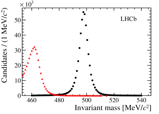
Figure 1: Mass spectrum for selected $K^{0}_{\rm\scriptscriptstyle S}\rightarrow\pi^{+}\pi^{-}$ candidates in the MB sample. The black points correspond to the mass reconstructed under the $\pi\pi$ mass hypothesis for the daughters, while the red triangles correspond to the mass reconstructed under the $\mu\mu$ mass hypothesis.

In order to further increase the background rejection, a boosted decision tree (BDT) [21] with the AdaBoost algorithm [22] is used. The variables entering in the BDT discriminant are:

• the decay time of the $K^{0}_{\rm\scriptscriptstyle S}$ candidate, computed using the distance between the SV and the PV, and the reconstructed momentum of the $K^{0}_{\rm\scriptscriptstyle S}$ candidate;

• the smallest muon IP $\chi^{2}$ of the two daughter tracks with respect to any of the PVs reconstructed in the event;

• the $K^{0}_{\rm\scriptscriptstyle S}$ IP $\chi^{2}$ with respect to the PV;

• the distance of closest approach between the two daughter tracks;

• the secondary vertex $\chi^{2}$, which adds complementary information with respect to the distance of closest approach of the tracks, as it uses information on the uncertainty of the vertex fit;

• the angle of the decay plane in the $K^{0}_{\rm\scriptscriptstyle S}$ rest frame with respect to the $K^{0}_{\rm\scriptscriptstyle S}$ flight direction, which is isotropic for signal decays, but not necessarily for background candidates;

• variables used to discriminate against material interactions, as further detailed below.

An important source of background consists of muons resulting from interactions between the particles produced in the PV and the detector material in the region of the VELO. The position of the SV of the background candidates from the $K^{0}_{\rm\scriptscriptstyle S}$ mass sidebands in the $x-z$ plane is shown in Fig. 2. The structures observed correspond to the position of the material inside the VELO detector. To discriminate against this background, two different approaches are used for the TIS and TOS trigger categories, consisting of two different choices of variables for the BDT.

For the TOS category, two additional variables are included in the BDT, the $p_{\rm T}$ of the $K^{0}_{\rm\scriptscriptstyle S}$ and a boolean matter veto that uses the VELO geometry to assess whether a given decay vertex coincides with a point in the detector material or not. Muons from material interactions have a harder $p_{\rm T}$ spectrum than muons from other background sources and hence are more likely to be selected by the trigger. The use of this variable in the BDT provides 50% less background yield for the same signal efficiency than simply applying the veto as a selection cut.

For the TIS category, the coordinates of the position of the SV in the laboratory frame are used to deal with this background. As the simultaneous use of the lifetime, $p_{\rm T}$ of the $K^{0}_{\rm\scriptscriptstyle S}$ meson, and the SV position allows the BDT to effectively compute the mass of the candidate, a fake signal peak could be artificially created out of the combinatorial background. Hence the $p_{\rm T}$ of the $K^{0}_{\rm\scriptscriptstyle S}$ meson is not used in the TIS analysis. This second approach provides a factor of two less background yield for the same signal efficiency than the matter veto (and $K^{0}_{\rm\scriptscriptstyle S}$ $p_{\rm T}$) for the TIS analysis, while, on the contrary, the matter veto boolean variable gives a factor of four less background yield for the same signal efficiency than the SV coordinates for the TOS analysis.

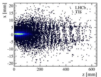
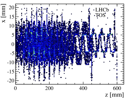
Figure 2: Position in the $x-z$ plane of the secondary vertices of the background candidates found in the high mass sideband for (left) TIS candidates and (right) TOS candidates. The lighter coloured areas correspond to higher density of points.

Because of these different approaches and to take into account the biases on the variable distributions introduced by the trigger, the data sample is split in two subsamples according to the TIS and TOS categories, for which BDT discriminants are optimised separately. In the TOS analysis, the $K^{0}_{\rm\scriptscriptstyle S}\rightarrow\pi^{+}\pi^{-}$ decays are required to have at least one of the daughters with a $p_{\rm T}$ above 1.3 ${\mathrm{\,Ge\kern-1.00006ptV\!/}c}$ in order to minimise the difference in the momentum distributions with respect to the triggered $K^{0}_{\rm\scriptscriptstyle S}\rightarrow\mu^{+}\mu^{-}$ candidates. The candidates that are simultaneously TIS and TOS are analysed only as TIS candidates to avoid counting them twice. Only one per mille of the TOS candidates overlap with TIS candidates.

In addition, the BDT discriminants for both trigger categories are defined and trained on data using $K^{0}_{\rm\scriptscriptstyle S}\rightarrow\pi^{+}\pi^{-}$ candidates as signal sample and $K^{0}_{\rm\scriptscriptstyle S}\rightarrow\mu^{+}\mu^{-}$ candidates in the upper mass sideband as background sample. For the background sample, the region above 1100 ${\mathrm{\,Me\kern-1.00006ptV\!/}c^{2}}$ (above the $\phi$ resonance) is used to define the BDT settings and the region between 504 and 1000 ${\mathrm{\,Me\kern-1.00006ptV\!/}c^{2}}$ to train the BDT algorithm chosen. For the signal sample, the $K^{0}_{\rm\scriptscriptstyle S}\rightarrow\pi^{+}\pi^{-}$ TIS events are used to train the BDT for the TIS category, while $K^{0}_{\rm\scriptscriptstyle S}\rightarrow\pi^{+}\pi^{-}$ decays with both pions misidentified as muons and passing the same trigger requirements as the $K^{0}_{\rm\scriptscriptstyle S}\rightarrow\mu^{+}\mu^{-}$ signal are used for the TOS category. In order to minimise the differences between misidentified $K^{0}_{\rm\scriptscriptstyle S}\rightarrow\pi^{+}\pi^{-}$ events and $K^{0}_{\rm\scriptscriptstyle S}\rightarrow\mu^{+}\mu^{-}$ decays, tight muon identification requirements (including cuts in the quality of the tracks or in the number of muon hits shared by different tracks) are applied to the $K^{0}_{\rm\scriptscriptstyle S}\rightarrow\pi^{+}\pi^{-}$ sample. These tight requirements are chosen such that the efficiency of the trigger in the $K^{0}_{\rm\scriptscriptstyle S}\rightarrow\pi^{+}\pi^{-}$ simulated decays is the same as in the $K^{0}_{\rm\scriptscriptstyle S}\rightarrow\mu^{+}\mu^{-}$ simulated decays.

In addition, the TOS and TIS categories are further split in two equal-sized subsamples, corresponding to the first and second halves of the data taking period. This procedure prevents possible biases related to the use of the same events in the mass sidebands both to train the BDT discriminant and to evaluate the background in the signal region, while making maximal use of the available data both for BDT training and background evaluation. Thus, in total, four different samples are defined (two subsamples for the TIS trigger category and two subsamples for the TOS trigger category) and combined as described in Sect. 7.

Candidates with low values of the BDT response are not considered because of the large amount of background in that region. This requirement provides about $50\%$ signal efficiency and $99\%$ background rejection, depending on the sample. The rest of the candidates are classified in ten bins of equal signal efficiency, i.e. a total of forty bins are combined to get the $\textrm{CL}_{\textrm{s}}$ limit.

4 Background

The search region is defined as the mass range $[492,504]$${\mathrm{\,Me\kern-1.00006ptV\!/}c^{2}}$. The background level is calibrated by interpolating the observed yield from mass sidebands ($[470,492]$ and $[504,600]$ ${\mathrm{\,Me\kern-1.00006ptV\!/}c^{2}}$) to the signal region. This is done by means of an unbinned maximum likelihood fit in the sidebands, using a model with two components. The first component is a power law that describes the tail of $K^{0}_{\rm\scriptscriptstyle S}\rightarrow\pi^{+}\pi^{-}$ decays where both pions are misidentified as muons; this model has been checked to be appropriate using MC simulation. The second component is an exponential function describing the combinatorial background. As an illustration, Fig. 3 shows the distribution of candidates for all BDT bins and for TIS and TOS samples, respectively. The expected total background yield in the most sensitive BDT bins of both samples ranges from 0 to 1 candidates.

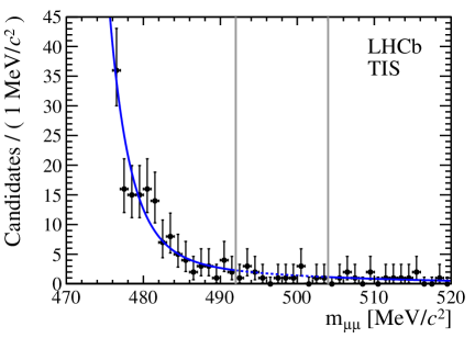
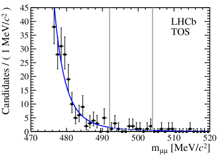
Figure 3: Background model fitted to the data separated along (left) TIS and (right) TOS trigger categories. The vertical lines delimit the search window.

Other sources of background, such as $K^{0}_{\rm\scriptscriptstyle S}\rightarrow\pi^{+}\mu^{-}\bar{\nu}_{\mu}$, $K^{0}_{\rm\scriptscriptstyle S}\rightarrow\mu^{+}\mu^{-}\gamma$, $K^{0}_{\rm\scriptscriptstyle L}\rightarrow\mu^{+}\mu^{-}\gamma$, $K^{0}_{\rm\scriptscriptstyle L}\rightarrow\pi^{+}\mu^{-}\bar{\nu}_{\mu}$ and $K^{0}_{\rm\scriptscriptstyle L}\rightarrow\mu^{+}\mu^{-}$ decays, are negligible for the current analysis. In the case of $K^{0}_{\rm\scriptscriptstyle L}\rightarrow\mu^{+}\mu^{-}$ and $K^{0}_{\rm\scriptscriptstyle L}\rightarrow\mu^{+}\mu^{-}\gamma$, the contributions have been evaluated using the ratio of the $K^{0}_{\rm\scriptscriptstyle S}$ and $K^{0}_{\rm\scriptscriptstyle L}$ lifetimes and the proper time acceptance measured in data with the $K^{0}_{\rm\scriptscriptstyle S}\rightarrow\pi^{+}\pi^{-}$ decays. The contributions of the other decay modes have been determined using MC simulated events.

5 Normalisation

A normalisation is required to translate the number of $K^{0}_{\rm\scriptscriptstyle S}\rightarrow\mu^{+}\mu^{-}$ signal decays into a branching fraction measurement. Two normalisations are determined independently for TIS and TOS candidates. The ${\cal B}(K^{0}_{\rm\scriptscriptstyle S}\rightarrow\mu^{+}\mu^{-})$ is computed using

$$\frac{{\cal B}(K^{0}_{\rm\scriptscriptstyle S}\rightarrow\mu^{+}\mu^{-})}{{\cal B}(K^{0}_{\rm\scriptscriptstyle S}\rightarrow\pi^{+}\pi^{-})}=\frac{\epsilon_{\pi\pi}}{\epsilon_{\mu\mu}}\frac{N_{K^{0}_{\rm\scriptscriptstyle S}\rightarrow\mu^{+}\mu^{-}}}{N_{K^{0}_{\rm\scriptscriptstyle S}\rightarrow\pi^{+}\pi^{-}}},$$ (2)

where, in a given BDT bin, $N_{K^{0}_{\rm\scriptscriptstyle S}\rightarrow\mu^{+}\mu^{-}}$ is the observed number of signal decays, $N_{K^{0}_{\rm\scriptscriptstyle S}\rightarrow\pi^{+}\pi^{-}}$ the number of $K^{0}_{\rm\scriptscriptstyle S}\rightarrow\pi^{+}\pi^{-}$ decays, and $\epsilon_{\pi\pi}/\epsilon_{\mu\mu}$ the ratio of the corresponding efficiencies. The efficiencies are factorised as $\epsilon=\epsilon^{\text{SEL}}\epsilon^{\text{PID}}\epsilon^{\text{TRIG/SEL}}$ where:

• $\epsilon^{\text{SEL}}$ is the offline selection efficiency. It includes the geometrical acceptance, reconstruction and selection, i.e, it is the probability for a $K^{0}_{\rm\scriptscriptstyle S}\rightarrow\pi^{+}\pi^{-}$ ($K^{0}_{\rm\scriptscriptstyle S}\rightarrow\mu^{+}\mu^{-}$) decay generated in a $pp$ collision, to have been reconstructed and selected;

• $\epsilon^{\text{PID}}$ is the efficiency of the muon identification for reconstructed and selected $K^{0}_{\rm\scriptscriptstyle S}\rightarrow\mu^{+}\mu^{-}$ signal decays;

• $\epsilon^{\text{TRIG/SEL}}=N^{\text{SEL\&PID\&TRIG}}/N^{\text{SEL\&PID}}$, where TRIG denotes either the TIS or the TOS categories, is the trigger efficiency for decays that would be offline selected. Under this definition, trigger efficiencies can be determined from data using the procedure described in Ref. [11].

The ratio of reconstruction and selection efficiencies between $K^{0}_{\rm\scriptscriptstyle S}\rightarrow\mu^{+}\mu^{-}$ and $K^{0}_{\rm\scriptscriptstyle S}\rightarrow\pi^{+}\pi^{-}$ decays is evaluated in bins of $p_{\rm T}$ and rapidity of the $K^{0}_{\rm\scriptscriptstyle S}$ meson using simulated events reweighted in order to reproduce the $K^{0}_{\rm\scriptscriptstyle S}$ $p_{\rm T}$ and rapidity spectra measured in data [23]. The reconstruction and selection efficiency for $K^{0}_{\rm\scriptscriptstyle S}\rightarrow\pi^{+}\pi^{-}$ decays is between 60% and 85% (depending on which point in the phase space a given event is from) of that of the $K^{0}_{\rm\scriptscriptstyle S}\rightarrow\mu^{+}\mu^{-}$ decays due to difference in the material interactions of the pions compared to muons.

The factor $\epsilon^{\text{PID}}$ is evaluated in bins of the BDT (both for the TOS and TIS categories) by measuring the muon identification efficiency as a function of $p$ and $p_{\rm T}$ using calibration muons. The sample of calibration muons is obtained from a $J/\psi\rightarrow\mu^{+}\mu^{-}$ sample in which positive muon identification is required for only one of the tracks. The $p$ and $p_{\rm T}$ spectra of the pions from $K^{0}_{\rm\scriptscriptstyle S}\rightarrow\pi^{+}\pi^{-}$ decays in a MB sample is later used to get the efficiency for $K^{0}_{\rm\scriptscriptstyle S}\rightarrow\mu^{+}\mu^{-}$ decays. The $\epsilon^{\text{PID}}$ efficiency is between $68\%$ and $82\%$ (depending on the BDT bin and the sample). It is measured with a precision between $1\%$ and $10\%$. For the ratio of trigger efficiencies, different strategies are considered for the TIS and TOS samples.

For the TIS samples, the $K^{0}_{\rm\scriptscriptstyle S}\rightarrow\mu^{+}\mu^{-}$ yield is normalised to the $K^{0}_{\rm\scriptscriptstyle S}\rightarrow\pi^{+}\pi^{-}$ TIS yield. In this case, the trigger efficiencies cancel in the ratio, because the probability to trigger on the underlying event is independent of the decay mode of the $K^{0}_{\rm\scriptscriptstyle S}$ meson. This cancellation is verified in simulation. The normalisation expression for TIS decays reads

$$\frac{{\cal B}(K^{0}_{\rm\scriptscriptstyle S}\rightarrow\mu^{+}\mu^{-})}{{\cal B}(K^{0}_{\rm\scriptscriptstyle S}\rightarrow\pi^{+}\pi^{-})}=\frac{\epsilon^{\text{SEL}}_{\pi\pi}}{\epsilon^{\text{SEL}}_{\mu\mu}}\frac{1}{\epsilon^{\text{PID}}_{\mu\mu}}\frac{N_{K^{0}_{\rm\scriptscriptstyle S}\rightarrow\mu^{+}\mu^{-}}^{\text{TIS}}}{N_{K^{0}_{\rm\scriptscriptstyle S}\rightarrow\pi^{+}\pi^{-}}^{\text{TIS}}},$$ (3)

where $N^{\text{TIS}}_{K^{0}_{\rm\scriptscriptstyle S}\rightarrow\mu^{+}\mu^{-}}$ and $N^{\text{TIS}}_{K^{0}_{\rm\scriptscriptstyle S}\rightarrow\pi^{+}\pi^{-}}$ are the number of TIS decays in a given BDT bin for signal and $K^{0}_{\rm\scriptscriptstyle S}\rightarrow\pi^{+}\pi^{-}$ modes respectively. $N^{\text{TIS}}_{K^{0}_{\rm\scriptscriptstyle S}\rightarrow\pi^{+}\pi^{-}}$ is found to be around 9000 for every BDT bin.

For the TOS sample, the $K^{0}_{\rm\scriptscriptstyle S}\rightarrow\mu^{+}\mu^{-}$ yield is normalised to the $K^{0}_{\rm\scriptscriptstyle S}\rightarrow\pi^{+}\pi^{-}$ yield from MB triggers. The normalisation requires in this case an absolute determination of the TOS trigger efficiency for $K^{0}_{\rm\scriptscriptstyle S}\rightarrow\mu^{+}\mu^{-}$, $\epsilon^{\text{TOS/SEL}}_{\mu\mu}$, as well as the knowledge of the average prescale factor of the MB trigger, $s^{\text{MB}}$. The absolute TOS trigger efficiency for the signal is computed using muons from $B^{+}\!\rightarrow J/\psi(\rightarrow\mu^{+}\mu^{-})K^{+}$ decays. The $p$ and $p_{\rm T}$ spectra of the $B^{+}\!\rightarrow J/\psi(\rightarrow\mu^{+}\mu^{-})K^{+}$ muons are reweighted in order to match those of pions from the $K^{0}_{\rm\scriptscriptstyle S}\rightarrow\pi^{+}\pi^{-}$ decays. Trigger unbiased $p$ and $p_{\rm T}$ spectra of the $K^{0}_{\rm\scriptscriptstyle S}\rightarrow\pi^{+}\pi^{-}$ decays can be obtained from the MB sample. The TOS efficiency is found to be at the level of 20% for all BDT bins. The normalisation expression for TOS decays reads

$$\frac{{\cal B}(K^{0}_{\rm\scriptscriptstyle S}\rightarrow\mu^{+}\mu^{-})}{{\cal B}(K^{0}_{\rm\scriptscriptstyle S}\rightarrow\pi^{+}\pi^{-})}=\frac{\epsilon^{\text{SEL}}_{\pi\pi}}{\epsilon^{\text{SEL}}_{\mu\mu}}\frac{1}{\epsilon^{\text{PID}}_{\mu\mu}}\frac{s^{\text{MB}}}{\epsilon^{\text{TOS/SEL}}_{\mu\mu}}\frac{N_{K^{0}_{\rm\scriptscriptstyle S}\rightarrow\mu^{+}\mu^{-}}^{\text{TOS}}}{N_{K^{0}_{\rm\scriptscriptstyle S}\rightarrow\pi^{+}\pi^{-}}^{\text{MB}}},$$ (4)

$N_{K^{0}_{\rm\scriptscriptstyle S}\rightarrow\pi^{+}\pi^{-}}^{\text{MB}}$ being the number of $K^{0}_{\rm\scriptscriptstyle S}\rightarrow\pi^{+}\pi^{-}$ decays from the MB trigger and $N_{K^{0}_{\rm\scriptscriptstyle S}\rightarrow\mu^{+}\mu^{-}}^{\text{TOS}}$ denoting the number of signal decays from the TOS category. $N_{K^{0}_{\rm\scriptscriptstyle S}\rightarrow\pi^{+}\pi^{-}}^{\text{MB}}$ is found to be around 1000 for every BDT bin.

The quantities

$$\alpha_{\text{TIS}}=\frac{\epsilon^{\text{SEL}}_{\pi\pi}}{\epsilon^{\text{SEL}}_{\mu\mu}}\frac{1}{\epsilon^{\text{PID}}_{\mu\mu}}\frac{{\cal B}(K^{0}_{\rm\scriptscriptstyle S}\rightarrow\pi^{+}\pi^{-})}{N_{K^{0}_{\rm\scriptscriptstyle S}\rightarrow\pi^{+}\pi^{-}}^{\text{TIS}}}$$ (5)

and

$$\alpha_{\text{TOS}}=\frac{\epsilon^{\text{SEL}}_{\pi\pi}}{\epsilon^{\text{SEL}}_{\mu\mu}}\frac{1}{\epsilon^{\text{PID}}_{\mu\mu}}\frac{s^{\text{MB}}}{\epsilon^{\text{TOS/SEL}}_{\mu\mu}}\frac{{\cal B}(K^{0}_{\rm\scriptscriptstyle S}\rightarrow\pi^{+}\pi^{-})}{N_{K^{0}_{\rm\scriptscriptstyle S}\rightarrow\pi^{+}\pi^{-}}^{\text{MB}}}$$ (6)

are called normalisation factors and are defined for each of the BDT bins. For a given number $N$ of $K^{0}_{\rm\scriptscriptstyle S}\rightarrow\mu^{+}\mu^{-}$ signal decays, the corresponding value of ${\cal B}(K^{0}_{\rm\scriptscriptstyle S}\rightarrow\mu^{+}\mu^{-})$ is then $\alpha\times N$. Using the value of ${\cal B}(K^{0}_{\rm\scriptscriptstyle S}\rightarrow\pi^{+}\pi^{-})$ from Ref. [4], the normalisation factors are in the range $[6.6,16.2]\times 10^{-8}$ for the TIS category, and $[0.9,7.8]\times 10^{-8}$ for the TOS category, depending on the BDT bin. From the normalisation factors, around $2\times 10^{-4}$ ($6\times 10^{-5}$) SM candidates are expected per BDT bin for the TOS (TIS) analysis.

6 Systematic uncertainties

The quantities considered in the determination of the branching fraction that are affected by systematic uncertainties are listed below.

• The background expectations per bin, obtained by comparing the results with the model described in Sect. 4 to those computed: a) if the combinatorial background is modelled by a linear function; b) if the mass range over which the fit is performed is modified; c) repeating the fit excluding (together with the signal region) the 12${\mathrm{\,Me\kern-1.00006ptV\!/}c^{2}}$ left and right windows neighbouring the search window and comparing the fit prediction to the yields in those regions; no correlation is considered among the different bins for this systematic uncertainty.

• The ratios of reconstruction and selection efficiencies and absolute muon identification efficiencies, for which systematic uncertainties are obtained from the difference between different methods in the data reweighting of the MC computed ratios and from the comparison to simulation respectively (around 20% for the ratios and 5% for muon identification efficiencies); no correlation is considered among the different bins.

• The branching fraction of the normalisation channel ${\cal B}(K^{0}_{\rm\scriptscriptstyle S}\rightarrow\pi^{+}\pi^{-})$ $=(69.20\pm 0.05)\%$ [4]; its uncertainty affects coherently the signal expectations of the forty bins of the analysis.

• The absolute TOS efficiency, for which the systematic uncertainty is obtained from the comparison to simulation (around 15%, depending on the BDT bin); no correlation is considered among the different bins.

• The effective prescale factor of the MB sample, $s^{\text{MB}}=(2.70\pm 0.76)\times 10^{-6}$. The uncertainty is evaluated from the difference between the prescale factor as measured in data and the value of the prescale as set in the trigger system. This systematic uncertainty affects coherently the signal expectations of the twenty bins of the TOS analysis.

The leading systematic uncertainties are those coming from the absolute TOS efficiency and $s^{\text{MB}}$ factor for the TOS analysis and from the ratio of reconstruction and selection efficiencies for the TIS analysis.

7 Results

The modified frequentist approach (or $\textrm{CL}_{\textrm{s}}$ method) [7, 8] is used to assess the compatibility of the observation with expectations as a function of ${\cal B}(K^{0}_{\rm\scriptscriptstyle S}\rightarrow\mu^{+}\mu^{-})$.

Test statistics are built from pseudo-experiments for the signal plus background and background-only hypotheses. For each pseudo-experiment a product of likelihood ratios is computed depending on the expected number of signal events for a given branching fraction, $s_{i}$, the expected number of background events, $b_{i}$ and the observed number of events, $d_{i}$ for bin $i$. The $\textrm{CL}_{\textrm{s+b}}$ ($\textrm{CL}_{\textrm{b}}$) is defined as the probability for signal plus background (background only) generated pseudo-experiments to have a test-statistic value larger than or equal to that observed in the data. The $\textrm{CL}_{\textrm{s}}$ is defined as the ratio of confidence levels $\frac{\textrm{CL}_{\textrm{s+b}}}{\textrm{CL}_{\textrm{b}}}$. This ratio is used to set the exclusion (upper) limit on the branching fraction, whereas $1-\textrm{CL}_{\textrm{b}}$ is used as a $p$-value to claim evidence or observation. A $95(90)\%$ confidence level exclusion corresponds to $\textrm{CL}_{\textrm{s}}=0.05(0.1)$.

The values of $b_{i}$ are obtained from the fit of the mass sidebands, as detailed in Sect. 4. The values of $s_{i}$ depend on the assumed branching fraction, as well as on the normalisation factors computed in Sect. 5. The uncertainties on the input parameters are taken into account by fluctuating the signal and background expectations when generating the $b$ and $s+b$ ensembles. These fluctuations are performed via asymmetric Gaussian priors, following the formula

$$x^{\prime}_{i}=x_{i}\left(1+\frac{1}{2}r(s_{+}-s_{-})+\frac{1}{2}r^{2}(s_{+}+s_{-})\right)$$ (7)

where $x_{i}$ is the central value of the parameter, $r$ is a random number generated from a normal distribution and $s_{+}$ and $s_{-}$ are the relative (signed) errors of $x_{i}$ [24]. Correlations are implemented by using the same value of $r$ for the parameters that should fluctuate coherently.

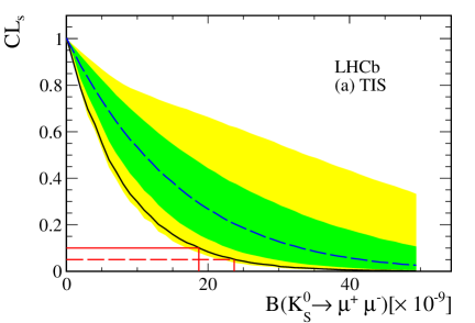
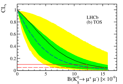
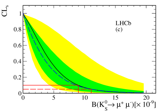
Figure 4: $\textrm{CL}_{\textrm{s}}$ curves for (a) TIS, (b) TOS categories and for (c) the combined sample. The solid line corresponds to the observed $\textrm{CL}_{\textrm{s}}$. The dashed line corresponds to the median of the $\textrm{CL}_{\textrm{s}}$ for an ensemble of background-alone experiments. In each plot, two bands are shown. The green (dark) band covers $68\%$ ($1\sigma$) of the $\textrm{CL}_{\textrm{s}}$ curves obtained in the background only pseudo-experiments, while the yellow (light) band covers $95\%$ ($2\sigma$).

Table 1: Upper limits on ${\cal B}(K^{0}_{\rm\scriptscriptstyle S}\rightarrow\mu^{+}\mu^{-})$ for the TIS and the TOS categories separately, and for the combined analysis. The last entry in the table is the $p$-value of the background-only hypothesis.

Quantity	TIS	TOS	Combined
Expected upper limit at 95 (90)% C.L. $[10^{-9}]$	$42\,(33)$	$13\,(10)$	$11\,(9)$
Observed upper limit at 95 (90)% C.L. $[10^{-9}]$	$24\,(19)$	$15\,(12)$	$11\,(9)$
$p$-value	0.95	0.20	$0.27$

The observed distribution of events is compatible with background expectations, giving a $p$-value of $27\%$. In particular, in the last 4 bins of the BDT output, corresponding to the most significant region of the analysis, just one candidate is observed in each of the trigger categories, in agreement with the background expectations. Figure 4 shows the expected and observed $\textrm{CL}_{\textrm{s}}$ curves for the TIS category and for the TOS category as well as for the combined measurement. The upper limit found is 11 (9)$\times 10^{-9}$ at 95 (90)% confidence level and is a factor of thirty below the previous world best limit. Table 1 summarises the limits in the TIS, TOS categories, and the combined result.

8 Conclusions

A search for $K^{0}_{\rm\scriptscriptstyle S}\rightarrow\mu^{+}\mu^{-}$ has been performed using 1.0 fb^-1 of data collected at the LHCb experiment in 2011. This search profits from the $10^{13}$ $K^{0}_{\rm\scriptscriptstyle S}$ produced inside the LHCb acceptance and the powerful discrimination against the $K^{0}_{\rm\scriptscriptstyle S}\rightarrow\pi^{+}\pi^{-}$ decay in which both pions are misidentified as muons, achieved thanks to the LHCb mass resolution for two body decays of the $K^{0}_{\rm\scriptscriptstyle S}$ meson. The candidates observed are consistent with the expected background, with the $p$-value for the background only hypothesis being $27\%$. The measured upper limit

$${\cal B}(K^{0}_{\rm\scriptscriptstyle S}\rightarrow\mu^{+}\mu^{-})<11(9)\times 10^{-9}$$

at 95(90)% confidence level is an improvement of a factor of thirty below the previous world best limit[3].

References

- [1] G. Ecker and A. Pich, The longitudinal muon polarization in , Nucl. Phys. B366 (1991) 189
- [2] G. Isidori and R. Unterdorfer, On the short distance constraints from , JHEP 01 (2004) 009, arXiv:hep-ph/0311084
- [3] S. Gjesdal et al., Search for the decay , Phys. Lett. B44 (1973) 217
- [4] Particle Data Group, K. Nakamura et al., Review of particle physics, J. Phys. G37 (2010) 075021
- [5] G. D’Ambrosio, G. Ecker, G. Isidori, and H. Neufeld, Radiative nonleptonic kaon decays, arXiv:hep-ph/9411439
- [6] KLOE Collaboration, F. Ambrosino et al., Search for the decay with the KLOE detector, Phys. Lett. B672 (2009) 203, arXiv:0811.1007
- [7] A. L. Read, Presentation of search results: the CLs technique, J. Phys. G28 (2002) 2693
- [8] T. Junk, Confidence level computation for combining searches with small statistics, Nucl. Instrum. Meth. A434 (1999) 435, arXiv:hep-ex/9902006
- [9] LHCb collaboration, A. A. Alves Jr. et al., The LHCb detector at the LHC, JINST 3 (2008) S08005
- [10] R. Aaij and J. Albrecht, Muon triggers in the High Level Trigger of LHCb, LHCb-PUB-2011-017
- [11] E. Lopez Asamar et al., Measurement of trigger efficiencies and biases, CERN-LHCb-2008-073
- [12] T. Sjöstrand, S. Mrenna, and P. Skands, PYTHIA 6.4 Physics and manual, JHEP 05 (2006) 026, arXiv:hep-ph/0603175
- [13] I. Belyaev et al., Handling of the generation of primary events in Gauss, the LHCb simulation framework, Nuclear Science Symposium Conference Record (NSS/MIC) IEEE (2010) 1155
- [14] D. J. Lange, The EvtGen particle decay simulation package, Nucl. Instrum. Meth. A462 (2001) 152
- [15] P. Golonka and Z. Was, PHOTOS Monte Carlo: a precision tool for QED corrections in and decays, Eur. Phys. J. C45 (2006) 97, arXiv:hep-ph/0506026
- [16] GEANT4 collaboration, J. Allison et al., Geant4 developments and applications, IEEE Trans. Nucl. Sci. 53 (2006) 270
- [17] GEANT4 collaboration, S. Agostinelli et al., GEANT4: A simulation toolkit, Nucl. Instrum. Meth. A506 (2003) 250
- [18] M. Clemencic et al., The LHCb simulation application, Gauss: design, evolution and experience, J. of Phys: Conf. Ser. 331 (2011) 032023
- [19] G. Lanfranchi et al., The Muon Identification procedure of the LHCb experiment for the first data, LHCb-PUB-2009-013
- [20] J. Podolanski and R. Armenteros, Analysis of V-events, Phil. Mag. 45 (1954) 13
- [21] L. Breiman, J. H. Friedman, R. A. Olshen, and C. J. Stone, Classification and regression trees, Wadsworth international group, Belmont, California, USA, 1984
- [22] Y. Freund and R. E. Schapire, A decision-theoretic generalization of on-line learning and an application to boosting, Jour. Comp. and Syst. Sc. 55 (1997) 119
- [23] LHCb Collaboration, R. Aaij et al., Measurement of production ratios in collisions at and 7 TeV, JHEP 08 (2011) 034, arXiv:1107.0882
- [24] R. Barlow, Asymmetric errors, eConf C030908 (2003) , arXiv:physics/0401042