Characterizing FaaS Workflows on Public Clouds:
The Good, the Bad and the Ugly

Abstract

Function-as-a-service (FaaS) is a popular serverless computing paradigm for developing event-driven functions that elastically scale on public clouds. FaaS workflows, such as AWS Step Functions and Azure Durable Functions, are composed from FaaS functions, like AWS Lambda and Azure Functions, to build practical applications. But, the complex interactions between functions in the workflow and the limited visibility into the internals of proprietary FaaS platforms are major impediments to gaining a deeper understanding of FaaS workflow platforms. While several works characterize FaaS platforms to derive such insights, there is a lack of a principled and rigorous study for FaaS workflow platforms, which have unique scaling, performance and costing behavior influenced by the platform design, dataflow and workloads. In this article, we perform extensive evaluations of three popular FaaS workflow platforms from AWS and Azure, running $25$ micro-benchmark and application workflows over $132k$ invocations. Our detailed analysis confirms some conventional wisdom but also uncovers unique insights on the function execution, workflow orchestration, inter-function interactions, cold-start scaling and monetary costs. Our observations help developers better configure and program these platforms, set performance and scalability expectations, and identify research gaps on enhancing the platforms.

1 Introduction

Serverless computing is a cloud computing paradigm for cloud application development, deployment, and execution without explicit user resource management. Function-as-a-service (FaaS) is a serverless variant where functions, triggered by events or requests, are the unit of application definition, deployment, and scaling. FaaS is widely used in enterprises [1], scientific computing [2, 3], and machine learning [4] due to its automatic elasticity, ease of management, and fine-grained billing per-invocation. We are also seeing the rise of FaaS Workflows, where functions are composed into a Directed Acyclic Graph (DAG) to form non-trivial applications with complex interactions [5]. Workflows form over $40\%$ of FaaS application deployments [6], and include public cloud offerings such as AWS Step Functions, Azure Durable Functions and Google Workflows.

1.1 Motivation and Gaps

A deeper understanding of the design, performance, and scalability of FaaS workflow platforms enables the development of better user applications and improves the utilization of FaaS platforms [6]. Applications that rely on low-latency performance and rapid scaling of FaaS functions may not necessarily achieve them for FaaS workflows. However, understanding the design trade-offs of these platforms is non-trivial for two reasons. First, commercial FaaS platforms from public Cloud Service Providers (CSPs) are proprietary. There is a lack of insight into the execution of a FaaS workflow. Developer documents have scarce details on their internal architecture, motivating the need for empirical studies for reverse engineering. Second, FaaS workflows have fine-grained and complex interactions between the functions through parameter passing, whose performance side-effects are not obvious [7]. The interplay between the platform architecture and workflow behavior is non-trivial.

Several recent efforts have conducted black-box profiling of FaaS platforms to understand their performance [6, 8, 9]. However, these are limited to individual functions, and these learnings do not fully translate to FaaS workflow platforms due to message passing and orchestration overheads, and the design choices on resource sharing and scaling in workflow platforms. Others have proposed FaaS benchmarks [10, 11, 12, 13, 14] to allow users to benchmark FaaS platforms. But these have not been composed into non-trivial applications with different lengths, branches, etc., relevant to us [15]. Lastly, there is a large body of research into optimizing FaaS platforms based on such experimental observations [16, 17, 18, 19]. Similar opportunities can arise based on our systematic study of FaaS workflow platforms [20].

In particular, there is a lack of a holistic study of diverse FaaS workflow characteristics to understand their performance, scalability, and costs on public clouds. We identify an exhaustive set of dimensions essential for developers and systems researchers to assess the workflow’s performance (functions and their compositions), understand their scaling, overheads due to container coldstarts, time spent on function execution vs. inter-function communication and coordination, and the monetary costs paid. These dimensions impact application behavior and are closely tied to the underlying CSP, requiring their characterization and analysis. Existing literature limits their study to just functions rather than workflows and/or only to a subset of these features (Table 1).

1.2 Contributions

We make several key contributions to address this gap.

1. We conduct a literature survey to define key dimensions to be analyzed to understand the performance of FaaS workflows (§ 2).

2. These dimensions guide our principled benchmarking study to characterize the performance and costs of three popular FaaS workflow platforms from AWS and Azure CSPs: AWS Step Functions and two flavors of Azure Durable Functions – Default Storage (AzS) and Netherite (AzN).

3. We analyze the outcomes of these benchmarks to examine features unique to FaaS workflows and use those to make a series of key observations. These complement, and sometimes contradict, the existing wisdom on FaaS functions and expose “the good, the bad, and the ugly” aspects of FaaS workflow platforms.

This article is the first its kind in-depth study to empirically evaluate and characterize FaaS workflow platforms on public clouds on such key dimensions. We have deployed $4$ FaaS workflows with $26$ functions and $159$ workload configurations on AWS and Azure for this study; cumulatively, the workflows are invoked $\approx 132k$ times and functions $\approx 5.8M$ times. This can help developers pick the best platform for their workload, cost and latency, and allow researchers to design and optimize better FaaS workflow frameworks. Some key insights include:

• Cold-start and Scaling: Our analysis shows the amplified effects of function cold-starts on workflows due to the workflow structure, e.g., the cold-start execution times of longer workflows is $\approx 74\%$ higher than warm-starts, while workflows with more task-parallelism see a $\approx 50\%$ higher cold-start overhead. AWS is able to scale faster than Azure.

• Inter-function vs. Function execution latencies: The time to transfer messages between the functions can dominate the workflow execution, taking $83$–$96\%$ of overall time. AzN has the least transfer latency for payloads up to $256KB$, while AzS has the highest. AWS has the least variability.

• Cost Analysis: FaaS workflow billing is complex with different components. Our models identify orchestration and data transfers as the dominant cost ($\approx$ 99%) rather than function execution. While AWS performs the best, it is also costlier.

We target the public FaaS platforms on Amazon AWS and Microsoft Azure, which account for $56\%$ of the cloud market. Others include Google Cloud Functions and IBM Cloud Functions. We use our XFaaS multi-cloud FaaS workflow deployment tool [21] to run realistic workflows and workloads from our XFBench workflow benchmark [15]. Provenance logs from XFaaS and cloud traces provide metrics for our analysis, and micro-benchmarks help analyze specific patterns.

The rest of this article is organized as follows: § 2 provides an overview of current research and gaps; § 3 reviews the design of FaaS workflow platforms from AWS and Azure; § 4 defines the workflow and workflow benchmarks used while § 5 describes our experiment harness. § 6 provides detailed results, observations, and insights from our study; and lastly, § 7 presents our conclusions and future directions.

2 Related Work

Table 1: Comparison of Literature on FaaS and FaaS Workflow Characterizations Studies

Lit. $\downarrow$ | Char. $\rightarrow$	Functions	Workflows	Scaling	Coldstarts	Func. Exec.	Inter-func.	E2E	Costs	CSPs
AOSP [22]						&	&		Knative, OpenFaas, Nuclio, Kubeless
BAOS [18]						&	&		Knative
CCSC [23]						&	&		AWS, Azure, Alibaba, GCP
CFOS [24]									IBM, AWS, Azure
CPES [25]									AWS, Azure
CSPS [26]									OpenFaas, AWS, FN Project
CTWS [27]						&	&		AWS, GCP, IBM
EPMS [28]						&	&		Azure
ESSW [29]									AWS, Azure, Alibaba, GCP
MOPCS [30]									AWS
MSSW [31]									AWS, Azure, Alibaba, GCP
PBCSP [9]						&	&		AWS, Azure, GCP
PCSW [32]									GCP
SITW [6]						&	&		Azure, OpenWhisk
WISEFUSE [33]									AWS, GCP, Azure
This Article									AWS, Azure
Examined, Partly examined, Not examined, & Not applicable since only functions are studied

2.1 Serverless and FaaS Characterization Studies

The proprietary nature of the commercial FaaS workflow platforms poses a significant impediment to understanding their performance trade-offs [7]. While they provide developer documentation and performance expectations, their detailed design and operational performance insights “in the wild” is rather limited [6]. Contemporary FaaS performance studies fail to offer a principled and rigorous evaluation of FaaS workflow platforms along key dimensions (Table 1).

2.1.1 Support for FaaS Functions vs. Workflows

This is a key distinction in our study, which goes beyond the performance of individual functions and holistically explores the behavior of workflows composed from them. Workflows have overheads of data transfers, orchestration, cascaded cold-start and scaling. Also, workflow costs vary for CSPs, and include non-trivial data transfer and orchestration costs.

Scheuner and Leitner [34] review articles between $2016$ and $2019$ and highlight research on the performance of FaaS functions on AWS Lambda. Our work extends to detailed first-hand performance and cost analysis of FaaS workflows on AWS and Azure. Microsoft Azure [6] characterize production workloads on Azure Durable Functions using the default storage provider (AzS). They analyze the function’s trigger types, invocation frequencies, patterns and resource needs. While $54\%$ of their applications have only $1$ function, $40\%$ have $2$–$10$ functions, forming FaaS workflows. $75\%$ of these functions execute within $10$s. The benchmark workflows in our study fall within this spectrum. While they focus on a CSP’s perspective to optimize their platform, we take a developer’s view in understanding these platforms and optimizing applications.

2.1.2 Scaling Properties

Rapid scaling is a unique benefit of FaaS. So, it is important to understand the responsiveness of FaaS workflow platforms to dynamic workloads. PBSCP [9], and CTWS [27] analyze the scaling performance of functions in managing sudden bursts of traffic. MSSW [31] extends this to FaaS workflows. They indicate that AWS is the best at scaling functions and workflows, and this matches our observations. Our study performs a more rigorous evaluation of the workflow scaling and the concurrency levels achieved on AWS, AzS and AzN for various workloads, and the consequent response times. We also analyze billed costs using a cost model.

2.1.3 Cold-start Overheads

Cold-start is the overhead paid for container initialization when scaling out in response to increased request rates to a function. These effects can cascade in workflows, and form an important metric for our analysis [27]. SITW [6] and PBCSP [9] show that cold-starts in AWS and Azure cause considerable delays in function execution. PBCSP suggests that GCP has the least cold-start latency and Azure has the most; we see similar behavior for Azure. BAOS [18] also propose optimizations to reduce cold-start latency. Our study analyzes the impact of these cascading overheads on workflows, and disaggregate function cold-starts and the inter-function data transfer overheads for a deeper insight on the variability of workflow executions.

2.1.4 Workflow Latencies

The end-to-end (E2E) execution time for workflows is an important user-facing metric. Understanding the effect of workflow patterns – number of functions, workflow length and number of fan-outs/fan-ins – on latency is critical [33]. The E2E time also includes overheads beyond function execution time, such as data transfers between adjacent functions and the workflow coordination. Studies like AOSP [22] examine function performance for Knative and OpenFaaS but lack an analysis of these additional latencies. CPES [25], CSPS [26] and WiseFuse [33] identify orchestration overheads and inter-function latencies as key factors of E2E latencies in AWS, Azure and OpenFaaS but do not analyze the impact of workflow structure, unlike us. Data transfer latencies can affect the E2E latency, depending on the payload sizes. WiseFuse [33] and CPES [25] suggest that inter-function overheads can be substantial and that Azure (AzS) performs particularly bad. We extend this comparison to Azure’s recent Netherite variant (AzN) and see better performance. We also establish the reasons for inter-function overheads based on the underlying system design, advancing prior research.

2.1.5 Monetary Cost Analysis

Lastly, the cost to execute the workflow is a vital metric for users but understudied. While this is simple for functions that are billed based on the memory usage and function invocation time (GB-s), workflows have complex execution and also opaque costing. Data transfer and coordination overheads are billed separately from function executions, and in fact dominate. CCSC [23] offers a cost breakdown for AWS, Azure, and Alibaba functions, but falls short on workflow insights. PCSW [32] and WiseFuse [33] both explore cost models for FaaS workflows for AWS and GCP, but fail to include data transfer costs that form the bulk of the cost. MOPCS [30] provides a cost analysis for AWS workflows, which is relatively simple and matches our model. Cost modeling for Azure is challenging since many granular moving parts that are billed separately.

2.2 Serverless and FaaS Benchmarks

Several FaaS and serverless benchmark suite have been proposed. However, they do no undertake a detailed study based on it. SeBS [12], FaaSdom [10], FunctionBench [11] and CrossFit [13] provide micro-benchmarks to determine system parameters such as CPU utilization, memory, disk I/O and network bandwidth. Only BeFaaS [35] and Deathstar [36] are application-centric benchmarks with complex interactions. BeFaaS, however, offers only a single eCommerce application and performs a limited empirical study with it, while Deathstar [36] is more for long-running serverless applications rather than FaaS workflows. FaaSScheduling [14] is a benchmark suite proposed to evaluate their performance-aware scheduler. However, it does not benchmark multiple FaaS platforms for different application workloads. Our recent work, XFBench [15], proposes a novel FaaS workflow benchmark that is deployed using our XFaaS multi-cloud FaaS framework [21]. But it only validates the workflow suite rather than perform a detailed analysis. This article leverages these prior works to perform an extensive characterization.

2.3 Research on Serverless and FaaS

There is a large body of work on optimizing FaaS platforms. Netherite [20] describes the design choices of the enhanced version of Azure Durable Functions, which we evaluate in this article. It partitions the application state for locality and uses storage efficient Azure Page and Block blobs. But there has been no detailed independent comparison of Netherite for FaaS workflows (Table 1). We contrast AWS Step functions, and Azure Durable Functions using both the default (AzS) and Netherite storage providers (AzN). Several works try to mitigate cold-starts in FaaS functions [37, 38, 39]. They typically optimize resource allocation, use pre-warming techniques and efficiently reuse containers for a faster response, while ensuring cost efficiency.

There is also research on optimizing FaaS platforms on private clouds, such as LaSS [40] and FaastLane [41]. Some build FaaS orchestration platforms from scratch, like Cloudburst [42] and Nightcore [43]. They mainly optimize the inter-function communication by co-locating dependent containers and using in-memory queues for transfers. We limit our study to public CSPs due to their wide adoption as compared to FaaS for private cloud [6].

3 AWS & Azure FaaS Workflow Platforms

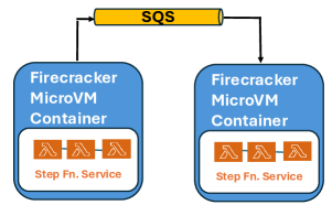
(a) AWS Lambda Step Functions

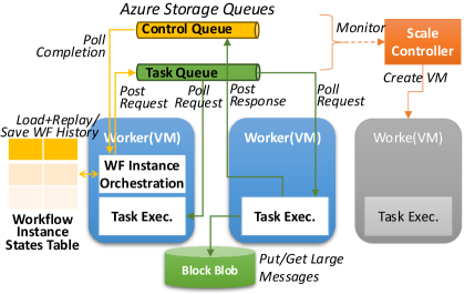
(b) Azure Durable Functions–Storage (AzS)

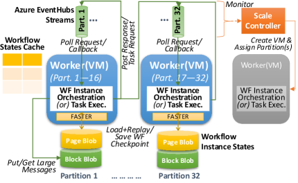
(c) Azure Durable Functions–Netherite (AzN)

Figure 1: Architecture of AWS (inferred) and Azure AzS and AzN FaaS Workflow Platforms.

Amazon’s AWS Lambda and Microsoft’s Azure Functions are two FaaS offerings that are widely used, and AWS Step Functions and Azure Durable Functions are thier corresponding FaaS workflow offerings. Azure has two variants: Azure Storage (AzS) and Netherite (AzN). Azure storage is the default “storage provider” for the Azure Durable Functions while Netherite [44] is more recent and achieves better performance.

3.1 Development and Deployment of FaaS Workflows

A developer designs a FaaS workflow by first defining the individual functions and then composing them into a workflow. AWS uses a YAML file for the workflow DAG while Azure requires custom orchestration code to be given. When deploying the workflow and its functions, users specify the data center and triggering mechanism for an invocation.

Once deployed, the functions of the workflow are in a “cold” state until a workflow invocation is received. On receiving the first request, the entry function’s execution environment is created in a new Firecracker microVM (AWS) or Worker VM (Azure), both of which we refer to as a container in this article. This container creation to execute the first function is a cold-start and the time taken is the cold-start overhead. Subsequent invocations may reuse existing containers, as discussed later.

The orchestration of the workflow execution is done through proprietary logic. This decides the next functions to execute based on the current execution state of a workflow invocation, and how to pass the output parameters from an upstream function as input parameters to the downstream function. It also decides when to scale containers up and down based on the load. These orchestrations are described next.

3.2 AWS Step Functions Orchestration

AWS Step Functions model workflows as state machines where each state is an individual step (function). A Step Function workflow defines the set of states and the conditions that determine how it transitions from one state to another.

AWS does not provide internal details for Step Function orchestration; the design in Fig. 1a is inferred based on empirical observations and other literature. Each function is an independent AWS Lambda function, implemented using Python, Java, Node.JS, etc., executing within a Firecracker container. The Step Functions service, which manages the execution of the state machine and tracks the current state, coordinates between them. When a Step Function is triggered it executes the workflow, transitioning between states based on the user logic. The trigger can happen from various sources in a synchronous, asynchronous or poll-based manner. Our experiments use an asynchronous REST call to invoke workflows. We surmise that Step Functions pass data between functions using Amazon Simple Queuing Service (SQS) based on Step Function’s 256KB limit on function data transfers, which matches the limit of AWS SQS.

AWS Step Functions inherit the scaling properties of AWS Lambda. Lambda starts a new container if a new function execution request is received and all current (warm) containers for that function are already executing a call . When a cold-start occurs [45], Lambda loads the container image into a Firecracker microVM from AWS S3 and serves the request once instantiated. The vCPUs allocated is proportional to the memory requested for the function by the user. Lambda is reported to handle up to $15,000$ concurrent cold-start events per second with $<50ms$ latency. Lambda limits each container to $10$ function executions per second, and the maximum concurrent containers to $1000$ per account. Prior works [9] indicate that AWS uses bin-packing for resource allocation to containers. The default timeout to scale down and unprovision a container that has not invoked a function is $5$ mins.

3.3 Azure Durable Functions Orchestration

An Azure Durable Functions workflow is composed programmatically by a user-defined orchestrator function, and user-defined activity functions that are invoked by the workflow. These are written in Python, .Net, JavaScript, etc. All activity and orchestrator functions run concurrently as processes in workers (VMs) that are shared among all functions of the workflow. Each VM has 2 cores and 1.5 GB of memory. We describe the two orchestration runtimes that Azure offers.

3.3.1 Azure Default Storage Provider (AzS)

AzS (Fig. 1b) is managed through a task hub, which is a collection of of several storage entities: Azure Tables to maintain the historical state of a workflow instance; Azure Control Queue to hold the state needed to invoke the next workflow step; Activity (Task) Queue to transfer the input parameter to activity functions if its size is $\leq$ 64KB; and Azure Blob storage to transfer larger messages.

A workflow instance is triggered by an HTTP request (used in our experiments) or a message from an Azure Queue. This creates entries in the control queue to asynchronously invoke the orchestrator and start the workflow. The orchestrator invokes the activity functions based on its control logic. It triggers an activity by writing its input payload to the history table, and publishes a message to the activity queue with the function’s input parameter (or a reference to a Blob entry for inputs $>64$KB). Any available worker for this workflow takes the message from the activity queue and executes the function on its VM. Multiple workers may concurrently execute functions from this queue. The function output is returned to the orchestrator using the control queue, which resumes execution and writes the output to the history table. The history table also helps the orchestrator decide the next downstream activity to execute. The orchestrator itself executes within these workers.

A Scale Controller scales out or in the number of worker VMs for the workflow. The unit of scaling is 1 VM, and there is a limit of $100$ VMs per workflow. The default timeout to shutdown idle VMs is 5 mins. It also replaces ‘slow’ workers with new worker.

3.3.2 Netherite Storage Provider (AzN)

Azure Netherite (AzN, Fig. 1c) uses Durable Task Netherite as the storage provider [44]. The overall orchestration pipeline is similar to AzS, but uses optimized storage services. This overcomes the scaling and latency limitations observed for queues, blobs and tables, instead using Azure Event Hubs, and Azure Page and Block Blobs. AzN uses in-memory and durable storage to persist durable events having the state changes in the orchestrations and activities.

AzN creates logical partitions to load-balance the activities across workers. Each partition is assigned Azure Page and Block Blobs to orchestrate and persist history, and Event Hubs for inter-partition communication. A worker VM handles one or more partitions, and the functions hosted on the worker read/write messages from/to Event Hubs on its partitions. The orchestrator writes its state and input/output messages to Page and Block Blobs in its partition. The Blobs are optimized for efficient I/O access using indexing by the FASTER database. The Scale Controller scales the number of partitions and workers, with a limit of 32 partitions and workers .

4 FaaS Workflow and Workload Suite

Table 2: Workflow Functions and Input Sizes: Small, Medium, Large

4.1 Functions and Workflows

While several FaaS function benchmarks exist [10, 11, 12, 13], few combine functions into meaningful workflows as practical applications [35]. Our recent XFBench [15] assembles popular functions from literature [10, 11, 12, 13, 14], along with our own, for a comprehensive suite of $26$ FaaS functions (Table 2). These cover compute-intensive numerical operations, graph algorithms with irregular access patterns, text processing of Enterprise data, and DNN/ML models for image analytics and inferencing.

We compose these functions into realistic workflow applications with diverse interaction patterns: Graph processing, Mathematical computation, Image analytics and Text processing (Fig. 2). The workflows also differ in their complexity: number of tasks ($5$–$25$), length of critical path ($3$–$7$), number of fan-ins and fan-outs ($2$–$20$), nested task parallelism ($0$–$2$), and take between ($1$–$900$ s) to run, depending on the workload. These also align with the workflow sizes observed in Azure deployments [6]. These workflow orchestration patterns affect the quantity of data flowing between functions, the number of concurrent tasks executed, the number of control logic/state transitions, etc., all of which affect the performance, scalability, overheads and costs of the FaaS workflow platforms.

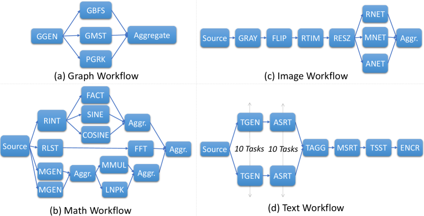
Figure 2: Workflow DAG Compositions from XFBench used in our study.

4.2 Workloads

Workloads determine the clients’ invocation pattern of the workflows. We consider three factors: the size of the input payload to the workflow, which has cascading effects on the size of downstream messages; the Requests per Second (RPS) sent to a workflow, and Dynamism in the RPS across time. We combine these to imitate real-world execution loads [6].

We use three payload sizes for each workflow: Small, Medium, and Large (Table 2). We use three static request rates for coverage: $1$ RPS, $4$ RPS, and $8$ RPS. While these are the rate to the initial function, fan-outs and fan-ins based on the workflow structure can increase the RPS on downstream functions. E.g., the text workflow executes $80$ concurrent TGEN downstream functions for an $8$ RPS workflow input. Lastly, we use three dynamic input rates: Step, Sawtooth, and “Alibaba”. Step sends the following RPS for $2mins$ each: $[1,2,4,8,4,2,1]$, slowly scaling up/down. Sawtooth has a sharper rise with these RPS for $10s$ each: $[1,2,3,4,5,6,7,8]$, and then drops to $0$ RPS for $60s$; this repeats thrice. Lastly, we scale and use the real-world Alibaba micro-services trace [46, 47] (Fig. 5f, red line), which has a peak of $17$ RPS. All workloads run for $5mins$, except Step that runs for $14mins$.

These are representative of enterprise, IoT and inferencing workloads. e.g., in IoT scenarios [48, 49] the workloads may be bursty (sawtooth) when sensors periodically send events with a similar frequency while eCommerce and user-facing workloads may show a gradual diurnal pattern (step).

5 Experiment Setup

5.1 Benchmarking Harness

XFBench [15] uses our open-source XFaaS framework [21] to implement the above functions and workflow DAGs in Python in a CSP-agnostic manner. XFaaS automatically generates each CSP’s native Python function wrappers with additional code to monitor function and workflow execution times, and translates the workflow DAG JSONs to the CSP’s workflow definition language. XFaaS also deploys these to specific CSP data centers. XFBench invokes the workloads on the deployed workflows using Apache Jmeter v5.6.2 load testing tool. All the workflows are HTTP triggered.

Besides the workflows and workload above, we also run micro-benchmark functions and workflows to evaluate specific characteristics of the FaaS workflow platforms.

5.2 Cloud FaaS Platform Setup

We refer to AWS Step Functions, Azure Durable Functions using the default Azure Storage Provider, and the more recent Azure Durable Functions using Netherite as AWS, AzS and AzN. We use data centers in the same region: ap-south-1 for AWS, and centralindia for Azure; select experiments are run in US-East and Central Europe. JMeter clients execute from an overprovisioned VM in the same data center to avoid wide-area network latencies an performance overheads. We use Standard D8s v3 VM with $8$ vCPUs and $32$GB RAM for Azure and EC2 C5.4X Large instance with $16$ vCPUs and $32$GB RAM for AWS.

We use the system defaults for all FaaS workflow platforms, unless noted otherwise. E.g., the maximum partition count (PC) in AzN is $12$, the maxConcurrentActivityFunctions (MA) in AzS is $10$, and the container timeout for both AWS and Azure are $5mins$. As discussed in 6.1 we change some defaults of AzS and AzN to ensure that most of the workflows and workloads can run. For AzS we change the maxConcurrentOrchestratorFunctions (MO) to $8$ and MA to $1$, and for AzN we change the PC to $32$. AWS Step Functions have no such knobs to tune. The container memory in AWS is set to $128MB$ for most function; we use $256MB$ for Alexnet and $512MB$ for Resnet to ensure the models fit. Azure does have a setting at a function level. We use the default Consumption Plan, which assigns $1.5GB$ memory and $1$ vCPU per worker VM.

5.3 Metrics

We measure, report and analyze key performance metrics from various logs in this characterization study. For each workflow invocation, we give the End-to-End (E2E) latency or makespan, which is the time between the start of the first function execution to the end of the last function execution along the critical path of that workflow. We also split this into the function execution times along the critical path and the inter-function times. These are measured by XFaaS using telemetry code introduced into the function logic, and using workflow ID/function sequence IDs introduced into the inter-function message headers. The time between the upstream function completing and the downstream function initiating is the inter-function time.

We also collect custom logs for our analysis, e.g., tracking the container IDs, CPU architectures, AWS Cloudwatch logs, and costing from the AWS and Azure portals. These help track cold-start overheads and the scale-in/-out of containers, in relevant analyses. For AWS, we get a count of the concurrent containers indirectly through the number of concurrent executions since only one executes per container, reported every $1min$. For Azure, our custom logger records the container ID and timestamps per execution to identify the number of unique workers and executions at any times for a workflow. For AWS, invocations that exceed the $95^{th}$ percentile of E2E execution time are classified as a cold-starts; all AWS runs have stable and reproducible E2E times and this way of detecting cold-starts suffices. For AzS and AzN, we detect the new containers on seeing a new container ID for an invocation.

6 Results

6.1 Scaling with Input Rates

A key defining feature of FaaS is its ability to scale the number of FaaS instances when the input load is variable and provide a stable latency. We examine if these properties extend to FaaS workflows and provide a stable E2E time.

Azure Durable Functions (AzS and AzN) are sensitive to configurations that affect concurrency and scaling, requiring tuning to achieve stable performance.

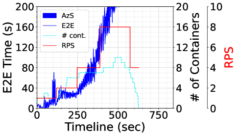
(a) AzS Default (MO=5, MA=10)

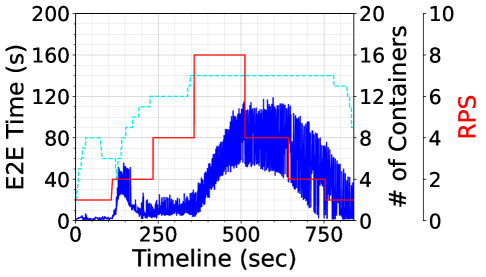
(b) AzS Custom (MO=8, MA=1)

Figure 3: AzS for Graph Workflow with Medium payload size and Step Workload, using different $MO$ and $MA$ configurations.

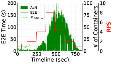
(a) Default, PC=12

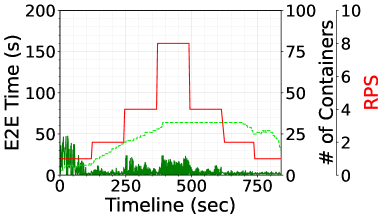
(b) Article, PC=32

Figure 4: AzN for Graph Workflow with Medium payload size and Step Workload, using two max. partition counts (PC) configurations.

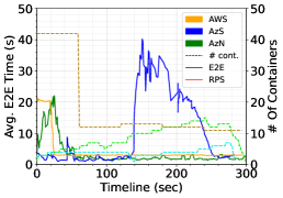
(a) Static 1 RPS

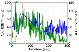
(b) Static 4 RPS

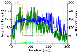
(c) Static 8 RPS

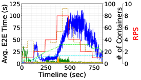
(d) Step

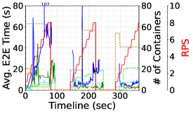
(e) Sawtooth

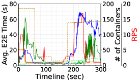
(f) Alibaba

Figure 5: Scaling performance of Graph workflow with medium payload and different input rates for AWS, AzS and AzN.

All executions for an AzS or AzN workflow share the same set of containers (VMs). The default settings to control container scaling use maxConcurrentOrchestratorFunctions ($MO=5$) and maxConcurrentActivityFunctions ($MA=10$), the orchestrator and function logic executions per container. However, this causes the Graph workflow to be unstable for a Step workload on AzS (Fig. 3a), i.e., the E2E execution time (dark blue line, left Y axis) spikes from $40s$ to $200+s$ as we reach 8 RPS (red line, right outer Y axis) leading to timeouts beyond the $490^{th}s$ (X axis). At the peak, $10$ containers (light blue dashed, right inner Y axis) are spun up by AzS to handle this load with $MA=10$ concurrent executions each. But each container is unable to handle 10 concurrent executions, causing functions to timeout.

We customize these to $MO=8$ and $MA=1$ to have one function per container but $8$ lighter-weight orchestrator executions. The scaling for AzS improves and complete the workload with $14$ containers (Fig. 3b). The peak latency stays within $110s$, though higher than the $<10s$ seen at a lower rates. While AzS can scale to $100$ containers, its cold-start behavior limits this growth (§ 6.2). The impact of these knobs are less acute for AzN. In the rest of the article, we default to $MO=8$ and $MA=1$ for AzS and AzN.

The maximum partition count ($PC$) for AzN decides the peak container count, as each container holds one or more partitions. The default $PC=12$ (Fig. 4, green dashed line, right inner Y axis) causes high variability in workflow execution times (green solid line, left Y axis), reaching $160s$ at $8$ RPS (red solid line, right outer Y axis). As PC is increased (Fig. 18 in Appendix), this gradually drops for $PC=32$ to a peak latency of $25s$, other than the initial cold-start. We use $PC=32$ for AzN in the rest of this article.

Overall, the control knobs in Azure affect the concurrency and scaling, which significantly impact the E2E latency. This forces developers tune the FaaS platform for their workload. In contrast, AWS scales well without such knobs, other than setting the function memory, which also affects its vCPUs [9].

AWS Step Functions scale up containers more rapidly and retain more active containers than Azure to quickly stabilize the E2E time. AzN is more responsive at scaling up than AzS but is limited by the peak number of containers. For stable workloads, AzN achieves comparable performance as AWS, but with fewer containers.

In Fig. 5, for the Graph workflow using a medium payload running on AWS and Azure, we report the E2E execution time (solid lines, left Y axis), the number of containers (dashed lines, right inner Y axis) and the RPS if dynamic (red line, right outer Y axis) over the invocation timeline (X axis). The E2E time is a sliding window average over $5s$ to smooth out spikes. AWS reports the number of containers only each $1min$.

6.1.1 Static Workflow Input Rates

AWS creates containers faster in response to concurrent invocations than Azure. E.g., comparing static RPS of $1$ and $8$ in Figs. 5a–5c, AWS spawns $42$ containers at the start (yellow dashed line) as it responds to the initial cold start delay, as seen from the higher execution times (yellow solid line) till the $20^{th}$ second. Once these calls catch up, the number of containers drops steadily but the execution time stays constant. This is seen for static $4$ and $8$ RPS too, where AWS initially spawns $148$ and $286$ containers before stabilizing to fewer container within $60s$. The E2E execution time for AWS is also much smaller than Azure at $4$ and $8$ RPS.

Azure starts with fewer containers and only gradually spins up more. For AzS at 1 RPS (Fig. 5a), it initially has $3$ containers (light blue dashed line) and this rises to $4$ after $32s$ and stays there, with a partially stable E2E time (solid blue line). However, a scale down at the $125^{th}$ second to $1$ container causes the E2E latency to spike, and it is unable recover till $250s$ by scaling up to $7$ containers. This is even slower for $4$ and $8$ RPS where the peak of $9$ and $16$ containers is reached only at $100s$, with E2E latencies growing till then. AzN has a similar trend, except that it scales more proactive and stabilizes the E2E time more quickly. E.g., for $4$ RPS (Fig. 5b) the number of containers (light green dashed line) grow to $12$ by $100^{th}$sec and rise to $21$ containers by $270^{th}$ sec, even as the latency steadily drops (solid green line).

6.1.2 Dynamic Workflow Input Rates

Figs. 5d–5f report the performance for dynamic workloads of the Graph workflow. AWS shows near-ideal scaling, as the number of containers (yellow dashed line) matches the varying RPS (red line). This is evident for Step and Sawtooth, where the container-count changes and stabilizes within $1min$ of the RPS change. Alibaba varies more quickly, and the container count loosely aligns with the RPS, partly due to the $1min$ reporting granularity. The E2E latency in all cases is small and stable at $2.9$–$3.0s$, beyond the initial $20s$ cold-start.

Azure is slower to respond to RPS changes, with AzN scaling containers faster than AzS to regain a low and stable E2E latency after an RPS increase. E.g., for Step (Fig. 5d), AzN ramps up twice as fast as AzS, reaching $32$ containers by $400s$ as RPS increases, compared to $14$ containers for AzS in the same period. AzS is unstable at the peak $8$ RPS and beyond. AzN’s E2E time of $2.9$–$3.1s$ is comparable to AWS even with only $32$ containers compared to AWS’s peak of $95$. This is because Azure scales based on the workflow’s performance rather than a function and VMs are shared by all functions, unlike AWS that scales for individual functions.

With Sawtooth (Fig. 5e), AzN’s container ramp-up is not fast enough for the first wave from $0$–$80s$, and it grows to $5$ containers as the E2E time spikes to $44s$. But for the second and third waves, the peak containers grow to $19$ to give a stable time of $2.9$–$3.1s$, which approaches AWS that launches $54$–$63$ containers. AzS is slower to ramp up and peaks at only $5$ containers and stabilize at a higher E2E time of $7.1s$.

Alibaba (Fig. 5f) has a higher variability and a peak of $17$ RPS at the end of the trace. AzN is unable to provide a low/stable latency, reaching $14.1s$, due to its $32$ container limit that is inadequate; AWS peaks at $150+$ containers with $3s$ latency. AzS is worse, with a latency of $45s$ with $12$ containers.

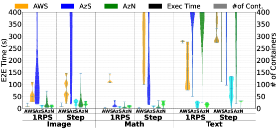
Figure 6: Scaling of Math, Image and Text workflows with medium payload for static 1 RPS and Step workloads.

6.1.3 Other Workflows

Lastly, Fig. 6 summarizes the scaling of the three other workflows for static 1 RPS and Step dynamic workload (detailed plots in Appendix Fig. 19). The Math, Image and Text workflows at static $1$ RPS are similar to earlier trends; AWS and AzN perform well, while AzS shows a more variable E2E time in the violin plot, especially for Image. For Step, AzS is unstable for all workflows beyond $2$ RPS and starts to timeout. It starts $11$ containers for Math workflow and uses $40$–$150$ for the more demanding Image and Text. Though AzS has a higher container limit than AzN, they are less effective. AWS and AzN handle Math and Image well for Step, though AzN shows a higher variability in time at the peak $8$ RPS even with $32$ containers. AWS spawns $40$–$120$ containers for these.

Text is the most demanding workflow. AzN is unstable beyond $2$ RPS for Step due to container limits. Even AWS shows variability at $8$ RPS as it reaches its limit of $1000$ containers , and its E2E latency doubles from $\approx 300s$ to $\approx 600s$ as multiple requests are concurrently sent to the same container, causing queuing.

6.1.4 Discussion

AWS scales rapidly within seconds to RPS changes and offers a stable E2E time. It also uses more containers, hitting its peak of $1000$, due per-function scaling raterh than per workflow. AzN performs well if RPS growth is slower, over minutes, and its E2E time approaches AWS – provided $32$ containers can handle the load. This limit prevents it from processing a demanding workloads. Scaling per workflow allows resource pooling across functions and using fewer containers than AWS. AzS performs worse than AzN and AWS, with slower scaling. It is unable to use its 100-container limit efficiently, and is unstable for several workloads.

6.2 Cold Start Overheads

One of the novel aspects of our study is to understand the cumulative effect of cold-starts for a workflow rather than just individual function cold-starts overheads studied earlier.

Azure Durable Functions (AzS and AzN) exhibit tangible cold-start overheads while it is negligible for AWS Step Functions

6.2.1 AWS Step Functions

The results from Fig. 5 and 6 show an absence of spikes in E2E workflow time for AWS other in the initial warmup period after deployment, which is limited $<20s$ as containers are rapidly spun up to handle the load. Since containers are retained for $5mins$, changes in container counts up to this initial peak and within $5mins$ do not cause a cold-start penalty.

E.g., in the Sawtooth workload of the Graph workflow (Fig. 5e), the initial wave starts $54$ containers causing an increase in E2E latency due to cold-starts; there is another negligible latency spike when this grows to $62$. But when containers drop to zero after wave one, and again grow to $52$ and $62$ for waves two and three, the containers warmed earlier are reused as it is within $5mins$. These low overheads are due to the fast startup of Firecracker microVMs, and optimizations such as sparse loading and deduplication of base images [45], with $<200ms$ cold-start overheads reported [50, 8].

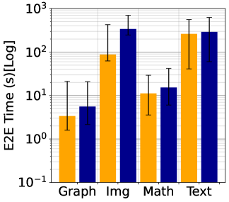
(a) AzS

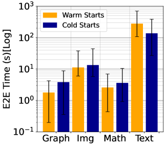
(b) AzN

Figure 7: E2E latency with and without container cold-starts, for all workflows with medium payload and 1 RPS. Whiskers show Q1–Q3 latency range.

(a) AzS

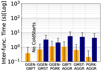
(b) AzN

Figure 8: Inter-function latencies with and without container cold-starts for AzS and AzN, for Graph workflow on medium payload and 1 RPS.

6.2.2 Azure Durable Functions (AzS and AzN)

Fig. 7 reports the E2E time for those workflow invocations with no cold-starts for any of their function invocations (only warm starts, yellow bar) and those that had one or more cold-starts (blue). This is shown for all four workflows using a medium payload and 1 RPS. The whiskers indicate Q1-Q3 latency ranges. Azure’s E2E time clearly varies with cold-starts, and is more variable than AWS as input rate changes. Azure workflow’s cold-start has three parts: (1) Container and runtime cold-start, the time to spawn a new container and load the Python runtime with dependencies from requirements.txt; (2) Function cold-start, the latency to run a function for the first time on a container, and lazily load the pending dependencies; and (3) Dataflow cold-start, the time to initialize data transfer services. These are discussed next.

Azure has a higher cold starts overheads for workflow with larger packages and larger payloads, though the container cold-start overhead is modest.

In Fig. 8, we zoom into the inter-function latencies between each pair of function in the graph and image workflows, and split them into warm-starts and cold-starts for the downstream function execution; this is shown only for function-pairs having one or more cold-starts. This inter-function latency is measured between an upstream function completing and the downstream function being invoked. This includes multiple components that we attempt to disaggregate.

The first time a container is created for the workflow, we have a container cold-start overhead that is included in this latency. We perform separate micro-benchmarks to measure this find it to be $\approx 290ms$ for AzS and $\approx 51.5ms$ for AzN, as described in the Appendix A.2.2. This overhead is modest.

The next component is a Python runtime cold-start overhead for the first time any function executes on a new container. This loads all the functions of the workflow and their dependent packages into container memory since the container is common to the workflow. It depends on the size of the packages, and should be constant for that workflow.So the inter-function overhead (Fig. 8, difference in blue and yellow bars) should be constant for different function-pairs since the container and runtime overheads are constant. However, this is seen to be variable. This is because of the dataflow coldstart.

We discern that the first time a message payload passes through the workflow, the system sets up necessary data transfer entities and connections for queues/blobs. For small payloads, this is through queues and for large ones through blobs, with the setup overheads being larger for the blob. E.g., Fig. 8 (and Appendix A.2, Figs. 21) shows the time for medium payload of Graph and Image that needs a blob and has higher/variable overheads. The corresponding overheads using queues for a small payload (Appendix, Fig. 20e and 20f) is smaller and stable at $\approx 4.1$s for Graph and $\approx 5$s for Image. Based on a microbenchmark (Appendix A.2), the Graph workflow using queues has $1s$ of dataflow overheads while blobs have $8.4$–$19.6s$. We are the first to report this.

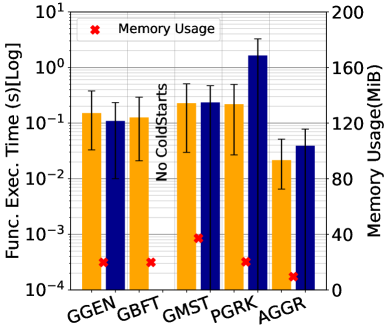
(a) Graph WF on AzN

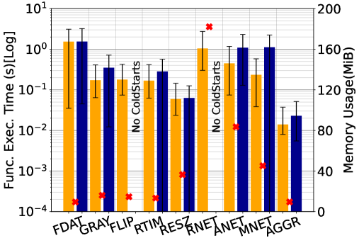
(b) Image WF on AzN

Figure 9: Function execution times with and without function cold-starts with medium payload and static $1$ RPS

The function cold-start overheads for Azure Durable Functions (AzS and AzN) depend on the size of dynamic packages and models.

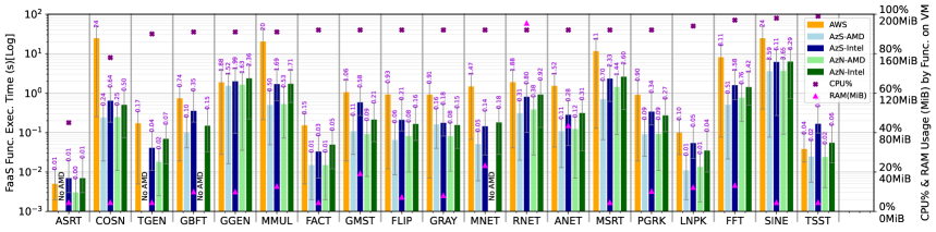
Figure 10: Function exection time within singleton workflow using medium payload input and static 1 RPS on AWS, AzS and AzN are shown as bars on left axis (log scale). CPU utilization% and Memory consumption (MiB) on Azure VM are shown as markers ($\times,\blacktriangle$) on right Y axis.

The function cold-start is paid for the first time a function executes on a container due to loading the dependencies lazily (e.g., Python imports) and models into the memory. Fig. 9 shows the user-logic execution time with and without cold-starts for the Graph and Image workflows on AzN (AzS is shown in Appendix A.2, Fig. 21). PGRK shows a penalty with cold/warm-start times of $\approx 1.1s/0.1s$ as it imports numpy and networkx packages (Fig. 9a). The other graph functions do not import these. The ML inferencing functions in the Image workflow load their ONNX models from disk and this ONNX session is retained for future warm-starts. In Fig. 9b, RNET, ANET and MNET have cold-start execution times that are $0.38$–$1.43$ s ($142$–$400\%$) higher than a warm-start.

Cold starts can impact workflow execution time in sequential workflows with cascading delays, but are less severe for workflows with parallel paths.

Image has the longest execution path and reports the highest cold start overhead for AzS and AzN due to cascading effects of workflow containers scale-up, with a penalty of $252s/74\%$ for AzS and $2.13s/16\%$ in AzN (Fig. 7). In contrast, the cold start overheads are more modest for Graph are $2.2s$ and $2.08s$ for AzS and AzN, and $4.01s$ and $1.03s$ for Math. This suggests that container may spin-up concurrently during first-time workflow execution for those with parallel paths. The package loading times also affect first-time function execution. For Text, the cold-starts are dwarfed by inter-function overheads due to large payloads, as discussed in 6.4.

6.2.3 Discussion

While function cold-starts are well studied [17, 51, 8], their impact on FaaS workflow are not. Our results indicate the need for more coordinated handling of cold-starts at the workflow level rather than for individual functions. In fact, through the use of shared VMs for functions in a workflow, Azure mitigates some of these overheads though its absolute time is higher than for AWS. Using function fusion can also potentially mitigate the impact for larger payloads [21].

6.3 Function Execution Times

We benchmark the functions used in the workflows individually within a “singleton” workflow having just one function. We also profile the CPU and memory usage of each function running on an Azure A1v2 VM with 1 x86 vCPU and 2GB RAM, as this is not reported from FaaS containers. Fig. 10 shows the FaaS function execution time (bars, left Y-axis), and their VM CPU% and memory usage (markers, right Y-axis).

Users assign memory limits to an AWS function that also decides the cores assigned to a container; we use 512MB and 2 vCPU cores per AWS container. AzS and AzN allocate a standard 1 core and 1.5GB of RAM per shared container. All three FaaS platforms run on x86 CPUs. cpuinfo shows AWS Lambda in this region run on older (2014) Intel Xeon E5-2680 v3 (Haswell) CPUs with $12$ cores at $2.5$GHz. Azure containers run on a mix of CPU models: AMD EPYC 7763 (Milan) with $64$ cores at $2.45$GHz (2021) and Intel Xeon E5-2673 v4 (Broadwell) with $20$ cores at $2.30$GHz (2016).

This has two implications.

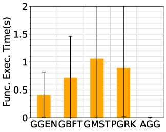
(a) Graph WF on AWS

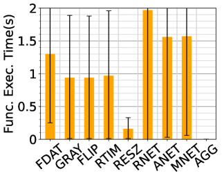
(b) Image WF on AWS

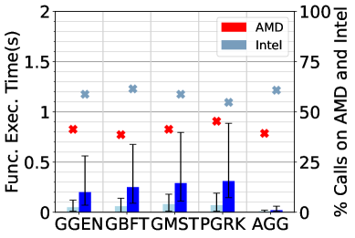
(c) Graph WF on AzS

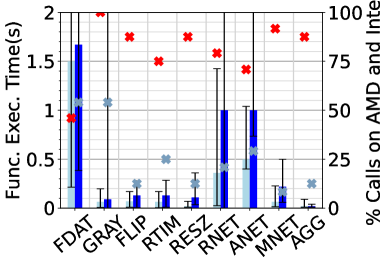
(d) Image WF on AzS

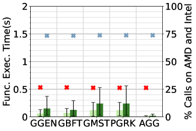
(e) Graph WF on AzN

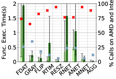
(f) Image WF on AzN

Figure 11: Function Execution Times for Graph (left) and Image (right) workflows on AWS, AzS and AzN, using medium payload and static 1 RPS.

Azure Durable Functions (AzS and AzN) usually execute functions faster than AWS Step Functions, especially for compute-intensive functions. CPU heterogeneity causes variable function performance within the same data center for AWS and Azure.

Given the newer CPU architecture of Azure containers, functions on Azure perform faster than AWS. This is seen in Fig. 10, where AWS functions take longer or are comparable to Azure functions. This is more acute for numerical functions such as matrix multiplication (MMUL), Page Rank (PGRK), FFT and ML inferencing (RNET, MNET, ANET), which benefit from the faster processors, e.g., PGRK on AWS takes $0.90s$, while for AzS and AzN it takes $\approx 0.09s$ on the AMD container and $\approx 0.30s$ on the Intel container.

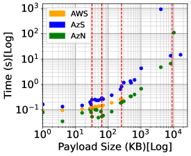
(a) All payload sizes (Log-Log plot)

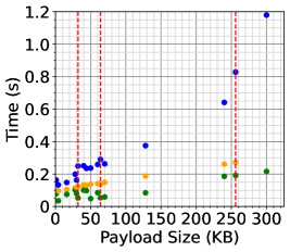
(b) Smaller payload sizes

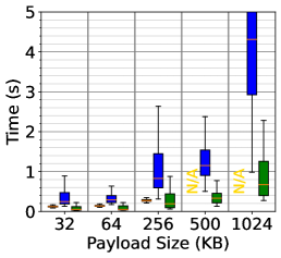
(c) Variability with payload size

Figure 12: Inter-function latencies for different payload sizes for micro-benchmark workflow.

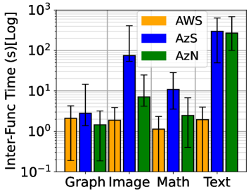
Figure 13: Inter-function latencies at 1 RPS and medium payload (cold starts omitted)

This hardware heterogeneity is also present in other global data centers, which impacts the performance of functions (Fig. 22 in Appendix A.3). In US East, AWS has 4 different CPU architectures for Lambda functions (Intel Xeon @ 2.5, 2.9 and 3GHz and AMD EPYC) while Azure has 3 Intel Xeon CPUs (E5-2673 v4 @ 2.3GHz, Platinum 8272CL @ 2.60GHz and Platinum 8171M @ 2.60GHz). In Central Europe, AWS has 3 Intel CPUs (Intel Xeon @ 2.5, 2.9 and 3GHz) while Azure runs only only 1 hardware type (AMD EPYC 7763).

Such function performance directly affects the E2E latencies of application workflows. In Fig. 11, we show function execution times for all functions of the Graph and Image workflows. These reaffirm that Azure functions perform faster than AWS functions. E.g., RNET in the Image workflow takes $1.99s$ on AWS while AzS and AzN take $\approx 0.4s$ on AMD and $1.2s$ on Intel. These cumulative function execution times also affect the E2E workflow latency, based on functions that lie on its critical path. This critical path functions time (excluding inter-function time) for Graph and Image workflows is slower of AWS at $2.19s$ and $5.78s$, and faster for Azure at $0.61s$ and $2.42s$ on AMD and $0.95s$ and $3.15s$ on Intel.

The CPU diversity also causes variability in the function execution times for a workflow. Further, containers for the same workflow can be from a mix of CPU types. The markers on the right Y axis of Fig. 11 show the mix of newer AMD and older Intel CPUs. This ranges from $10:90$ (Image on AzN) to $60:40$ (Image on AzS) for a given workflow run. The execution time difference on these CPUs is high as $3\times$, consequently affecting the workflow E2E times for different runs of the same workflow. In this region, AWS happens to use the same CPU model for containers, with stable performance.

Figure 14: Distribution of the number of functions executing per container in a 300 sec window for AzS and AzN for Medium payload and static $1$ RPS.

Azure Durable Functions (AzS and AzN) have more variability in function execution times as compared to AWS Step Functions.

Besides CPU heterogeneity, Azure has variability due to the allocation of function executions to each container of a workflow. AzS uses a common activity queue that containers poll for the next task while AzN partitions the tasks across queues maintained for each partition. Fig. 14 shows a violin distribution of the number of functions executed per container during a $5mins$ window for each workflow. The tighter this violin, the more balanced the function executions are across containers, and lower the value, the less load each container has. AzS shows a higher variability for Graph than AzN, while for Image, both are comparably lower at a median of $\approx 75$ tasks. This suggests that AzN achieves better load-balancing, reducing the variability of function execution times. The distribution is even more dispersed for complex workflows like Math and Text. In contrast, AWS executes only one function per container and avoids such load-balancing skews, albeit using more container resources.

6.4 Inter-function Communication Times

The inter-function latency is small for payloads $\leq 100KiB$ between functions on all platforms, with AzN performing the best and AzS the worst. AzS and AzN exhibit greater variability in transfer latency compared to AWS.

We perform micro-benchmarks with a simple workflow having a function that just transfers a fixed-size payload to the next function. Fig. 12 reports the inter-function time, from the end of the first function to the start of the next function’s logic. A box plot and median values over $120$ invocations are shown. We omit cold-start outliers. The time taken for smaller payloads $\leq 100KiB$ is small (Fig. 12b): $\leq 100ms$ for AzN, $\leq 150ms$ for AWS and $\leq 300ms$ for AzS.

For $\leq 256KiB$, AWS Step Functions are expected to use a queue-based mechanism, and the transfer times are dominated by the network latency than bandwidth limits. For larger messages, developers need to use custom means, e.g., by storing and loading from AWS S3 files, which limits the intuitiveness of Step Functions. That said, the inter-function latency for AWS is linear for the smaller payload sizes.

AzS uses Azure Queues for payloads $\leq 45KiB$, which when base64 encoded grows to the $64KiB$ message size limit. For larger payloads, it automatically switches to Azure Blobs by compressing and asynchronously uploading the payload and internally passing a reference to the downstream function using Queues, where they are restored. This transition to Blobs affects the performance, and we see the slope change past $45KiB$ (Fig. 12b); this further degrades at $256KiB$ (Fig. 12a) due to the way Blobs are handled.

AzN uses Azure Event Hubs, with better performance than Queues, for smaller payloads up to $9000KiB$ and Blobs for larger ones. Interestingly, they split smaller messages into $30KiB$ events and larger payloads into $500KiB$ files, and use parallel and asynchronous transfers. So AzN is uniformly faster than AWS and AzS (Fig. 12b) until $9000KiB$ (Fig. 12a), when it switches to Blobs and the latency rises.

We also see that the variability for the inter-function latencies is tight for AWS, for the payload sizes it supports (Fig. 12c). In contrast AzS and AzN exhibit high variability and this deteriorates for larger payload sizes. The use of Blobs files in AzS and the splitting and rejoining of messages in AzN causes variability for larger payloads. AzS and AzN exhibit failures for a larger payload transfers of $\geq 4MiB$; at $16MiB$, failures during transfers are routine.

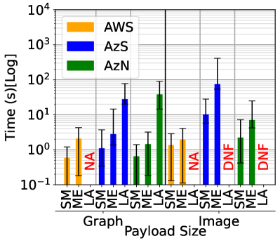
(a) Payload varies

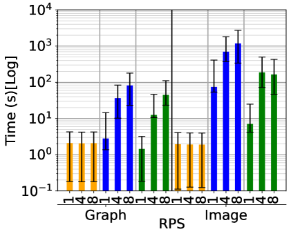
(b) RPS varies

Figure 15: Inter-function latencies for Graph and Image workflows while varying Payloads and RPS (omitting cold-starts)

As the workflow length increases, the inter-function latency significantly increases in AzS and AzN, this is less pronounced in AWS.

Fig. 13 shows the median inter-function latencies (log scale) on the workflow’s critical path, i.e., directly contributes to the E2E time. The error bars indicate Q1–Q3 values over 300 invocations ($300s$). The length of the workflow significantly affects the inter-function latencies. E.g, both Graph and Image have similar fan-out degrees and payload sizes but Image is longer than Graph (Fig. 2). For Graph, AzS has the highest median latency ($2.9s$) and AzN the least ($1.2s$), while AWS is at $2s$. In contrast, Azure latencies for Image are much higher at $73s$ for AzS and $6s$ for AzN, while comparable for AWS at $2s$. In Azure, before every function execution, the entire workflow history is retrieved and this increases with longer paths. This is observed for Image and Text where the last two edges on average take $3.2s$, $52.38\%$ more than the first two edges. AzS uses Azure Storage Tables that are slower than AzN that uses the in-memory table for orchestrators. Math and Text have larger fan-out degrees of 6 and 10. Here, AzS and AzN both incur larger inter-function overheads compared to AWS at $1s$, $10s$, and $2.1s$ for Math on AWS, AzS, and AzN, and $1.95s$, $300s$, and $297s$ for Text.

AWS consistently outperforms both AzS and AzN across all workflows, except for Graph, where AzN is slightly faster. For Graph, AWS is 40% faster than AzS ($2s$ vs. $2.9s$), but AzN is actually $40\%$ faster than AWS ($1.2s$ vs. $2s$). For Image, AWS is $97\%$ faster than AzS ($2s$ vs. $73s$) and $67\%$ faster than AzN ($2s$ vs. $6s$). This suggests that AWS does a more efficient inter-function data transfer, maintaining stable latency even as workflows increase in node count and path length. AzS consistenyl performs worse than AzN, with $2.4\times$ higher latency in Graph, $12\times$ in Image, and nearly $5\times$ in Math, and more so for complex workflows.

Increasing payload sizes causes a linear increase in inter-function latency for AWS, within its $256KB$ limit. For AzS and AzN, it leads to higher variability in inter-function times, and sometimes failures, for larger workflows.

We examine the effect of using different payload sizes and RPS on the inter-function latency. Fig. 15 shows the median inter-function latency (with error bars indicating Q1–Q3 values) for the Graph and Image workflows when we vary the payload (retaining $1$ RPS) or vary the RPS (retaining a medium payload). For the large payload, AWS does not support these sizes while Azure gives timeout errors for Image (DNF).

In the Graph on AWS, the inter-function latencies increase from $0.59s$ to $2.09s$ as we switch from small ($47KiB$) to medium payload ($220KiB$), which is a $3.5\times$ increase, while for Image this increases from $1.37s$ to $1.94s$ for small $39KiB$ to medium $245KiB$: a $1.41\times$ increase. On average the increase is about $\approx 2.4\times$. This is consistent with the microbenchmarks (Fig. 12b), where we see a $\approx 2.07\times$ increase when the size increases from $45KiB$ to $250KiB$.

For Graph/Image on AzN, going from small ($47KB$/$39KB$) to medium ($220KB$/$245KB$) is an $\approx 5\times$ increase in payload and causes a somewhat linear increase in time for AzN ($0.55s\rightarrow 1.45s$/$2.23\rightarrow 7.09s$) which is about $2.63\times/3.17\times$. This too is consistent with the microbenchmarks (Fig. 12b) where we see an increase of $\approx 2.85\times$ in inter-function time from $45KiB$ to $250KiB$. For AzS, this payload size change causes a switch from Queues to Blobs. Here, the impact is worse for Image ($10s$ to $74s$, $7.4\times$) due to its longer path, causing more requests per second to the common Blob storage. AzN’s use of Event Hubs even for medium sizes mitigates this.

When we move from medium to large payload ($1.1MB$, $\approx 5\times$ increase), the increase in time is super-linear and sharper for Graph on both AzS ($27s$) and AzN ($38s$), and worse than the latency increase seen in the micro-benchmarks for comparable payload sizes. Larger payload sizes cause greater stress on the storage accounts in writing and reading the inter-function messages. This is exacerbated as the workflow size and latency growth since more operations happen concurrently for multiple executing workflows. The large payload for Image workflow also causes frequent failures. Hence, for larger and more complex workflows the inter-function latency growth is much worse than seen in the micro-benchmarks for AzS and AzN (Fig. 12), limiting workflow scalability.

Inter-function latencies for AWS is not sensitive to the request rate, while AzS and AzN show an increase with the rate, limiting their scalability.

As the RPS increases $1$ to $8$, there is no increase in the inter-function latencies on AWS from for both Graph and Image (Fig. 15b), remaining at $2s$ for Graph and $1.9s$ for Image. Hence, irrespective of the workflow structure, the inter-function performance of AWS scales well with increasing rate. This, along with the favorable cold-start scaling (6.2) and sandboxed function performance (6.3), leads to overall positive scaling performance of AWS FaaS workflows with input rate (5).

However, for AzS and AzN, a rise in RPS translates to more frequent payload transfers and importantly, a greater number of orchestrator operations within the same time period. The AzS and AzN orchestrators perform several lookups and updates on the workflow history between two function calls, stressing the storage accounts. E.g., for Graph, when we go from 1 RPS to 4 RPS, AzS goes from $2.3s$ to $36s$, and AzN from $1.45s$ to $12s$, which are more than $4\times$. This is similar for Image as well, with AzS increasing by $87.5\times$ and AzN by $28.5\times$.

Overall the inter-function latencies are lesser for AzN than AzS for both Graph and Image workflows as it benefits from the partitioning ($PC=32$) of messages to separate queues, one per worker. In contrast, AzS uses Storage Queues to transfer messages and Storage Tables for the workflow state updates, both of which perform and scale poorly.

6.5 Workflow Execution Times

With an increase in the workflow length, the end-to-end latency significantly increases in AzS and AzN both, while the effect of length is less pronounced in AWS, mostly due to the increased inter-function overheads. An increase in the degree of parallelism has little impact on the end-to-end latency for AWS, while this latency increases in AzS and AzN, both.

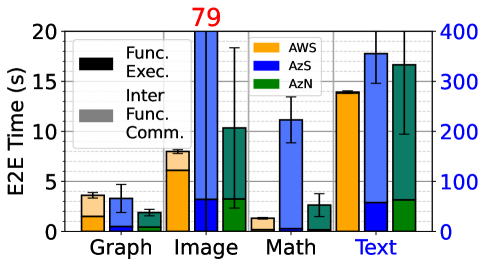
Figure 16: E2E WF execution time on Medium Payload, 1 RPS.

Here we examine the time spent along the critical path of the workflow, i.e., path in the workflow from the source function to sink function that takes the maximum execution time. Fig. 16 reports the E2E time of the four workflows at 1 RPS for medium payload. This time is split into the function execution latencies (bottom stack) and inter-function latencies (top) along the critical path. We run these for $5mins$ at 1 RPS for medium payload and omit the coldstart overheads.

For 3 out of 4 workflows – Image, Math and Text – AWS has the least workflow E2E times at $8.0s$, $1.3s$ and $278s$, and is $22.8\%$, $50.1\%$ and $16.4\%$ faster than AzN, the next best. For all four workflows, AWS has lower inter-function latency, as we saw earlier for medium payload and 1 RPS (§ 6.4). However, its function execution times are slower than AzN and AzS for Image and Text, and comparable to AzN on Math. The net effect results in these E2E times. AWS is slower than AzS and AzN for Graph, taking $3.6s$ or $91.6\%$ more than AzN, due to much slower function execution time. In general, function execution times tend to dominate for AWS, taking $52$–$96\%$ of the total E2E times for Graph, Image and Text workflows, with ENCR in Text taking $\approx 280s$ or $99.3\%$ of total time. These are consistent with our results in § 6.3.

On the other hand, Azure runtimes are dominated by inter-function latencies that account for $83$–$96\%$ of E2E times for all workflows. AzN is faster than AzS for all workflows, by $42.9\%$, $86.7\%$, $50.1\%$, and $6.3\%$ for Graph, Image, Math and Text. AzN usually has lower inter-function latencies due to better storage performance, and it function execution times are comparable or sightly better than AzS (Fig. 10).

In summary, our earlier piece-wise observations on the function execution and inter-function latencies come together to impact the E2E workflow latency, and the net result is consistent with earlier expectations. This confirms that our analysis can extend to other workflows and workloads as well.

6.6 Cost Analysis

Cost is a key factor in using cloud services. While AWS Step Functions have a simple and transparent costing, Azure’s costs are complex to compute and have not been investigated before. We develop a cost model to help arrive at an accurate costing and analyze these across our workflows.

The cost for a workflow invocation has three parts: function execution costs ($\alpha$), inter-function transfer costs ($\beta$), and workflow orchestration costs ($\gamma$), with the total cost $\kappa=\alpha+\beta+\gamma$. Let a given workflow have $n$ functions and $e$ dataflow edges between them. Let the function execution times (seconds) be $t_{1},t_{2}\cdots t_{n}$, and their configured memory (GB) be $m_{1},m_{2}...m_{n}$. Say the data transfer sizes (GB) on each edge is $D=\{d_{1},d_{2}...d_{e}\}$, with the input to the workflow being $d_{0}$.

6.6.1 AWS Cost Model

For AWS, each function execution is billed based on the memory assigned to the container and function execution time. The total function execution cost is $\alpha_{aws}=k^{func}_{aws}\times\sum_{1\leq i\leq n}(t_{i}^{aws}\times m_{i})$. Here, $k^{func}_{aws}$ is the cost per GB-sec of the function execution, and depends on the data center and container type (e.g., x86, ARM, etc.). AWS does not separately bill for inter-function payload transfers since message sizes have a small upper-bound and only bills for orchestration costs of $k^{xfr}_{aws}$ for every $1000$ state transitions in the Step Function. Hence, we set $\beta_{aws}=0$ and compute the orchestration costs from the number of workflow state transitions, $\gamma_{aws}=\frac{k^{xfr}_{aws}\times e}{1000}$. So, the total AWS cost is:

$$\kappa_{aws}=\big(k^{func}_{aws}\times\sum_{1\leq i\leq n}(t_{i}^{aws}\times m_{i})\big)+\Big(\frac{k^{xfr}_{aws}\times e}{1000}\Big)$$

where $k^{func}_{aws}=\mathdollar 0.00001667$ per GB-sec and $k^{xfr}_{aws}=\mathdollar 0.0285$ per state transition for our experiments.

6.6.2 AzS Cost Model

The function execution cost for AzS is similar to AWS, $\alpha_{azs}=k^{func}_{azs}\times\sum_{1\leq i\leq n}(t_{i}^{azs}\times m_{i})$, with a cost coefficient of $k^{func}_{azs}=\mathdollar 0.000016$ per GB-sec for our data center. One thing to note here is, Azure does not have a notion of ‘containers’, it instead spins up VMs, that may run multiple functions in the same VM. Hence, for Azure, the memory used by functions is calculated from the XFaaS provenance logs.

The inter-function costs for AzS depends on the data transfer size between the two functions, and differ based on whether Queues are used ($<45KB$) or Blobs ($\geq 45KB$). Let the total number of edges in the DAG with less than $<45KB$ of data transfer sizes be $e_{q}=|d_{i}|\penalty 10000\ \forall d_{i}<45KB\in D$. We are billed for each put and get operations of these messages on the queue at $k_{azs}^{qtxn}$ for every $10k$ operations. Let those edge with sizes $\geq 45KB$ be $e_{b}=e-e_{q}$, and let the sum of the data transfers on these edges be $d^{xfr}_{blob}=\sum_{\forall d_{i}\geq 45KB}d_{i}$. $d_{0}$ will be included in $d^{xfr}_{blob}$ if the input payload size is greater than $45KB$; else it will increment $e_{q}$. We are billed for each Blob put and get operations at $k_{azs}^{bput}$ and $k_{azs}^{bget}$ for every $10k$ operations, and also for the GB read and written at $k_{azs}^{brw}$ per GB. So, the inter-function transfer costs is:

For our setup, we have $k_{azs}^{qtxn}=\mathdollar 0.0004$, $k_{azs}^{brw}=\mathdollar 0.02$, $k_{azs}^{bput}=\mathdollar 0.065$ and $k_{azs}^{bget}=\mathdollar 0.005$.

Lastly, the orchestrator uses Azure Storage Tables to write the input and output of every function. The total data (GB) written and read is: $d^{orch}_{tbl}=d_{0}+\big(2\times\sum_{1\leq i<n}d_{i}\big)+d_{n}$, with the initial ($d_{0}$)/final ($d_{n}$) payloads only being written/read, with a cost of $k_{azs}^{trw}$ paid for every GB. There are also read and write costs for the tables at each of the $n$ DAG vertices, billed for every $10k$ transactions. The orchestration cost is:

$$\gamma_{azs}=k_{azs}^{trw}\times d^{orch}_{tbl}+k_{azs}^{ttxn}\times\frac{2\times n}{10000}$$

For our setup, we have $k_{azs}^{trw}=\mathdollar 0.045$ and $k_{azs}^{ttxn}=\mathdollar 0.0004$.

6.6.3 AzN Cost Model

The function execution cost for AzN is identical to AzS, $\alpha_{azn}=\alpha_{azs}$. Inter-function data transfers in AzN happens through Event Hubs for up to $9000KiB$ in size. Its pricing depends on the send and receive bandwidth usage, billed at $k^{ehbw}_{azs}$ for every throughput-unit (TU) used. Each TU offers an average of $1MB/s$ of receive and $2MB/s$ of send bandwidth in an hour. The total payload sent and received (in GB) across all edges of the DAG is $d^{xfr}_{ehub}=\sum_{0\leq i\leq n}d_{i}$. If $t_{e2e}$ is the E2E workflow execution time for the invocation (in seconds), the average receive TUs used for the workflow is $\frac{d^{xfr}_{ehub}\times 1000}{t_{e2e}/3600}$, and the send TUs is $\frac{d^{xfr}_{ehub}\times 1000}{2\cdot t_{e2e}/3600}$. So the data transfer cost is the larger of the two, i.e., the former:

$$\beta_{azn}=k^{ehbw}_{azn}\times\frac{d^{xfr}_{ehub}\times 1000}{t_{e2e}/3600}$$

In our experiments, $k^{ehbw}_{azn}=\mathdollar 0.015$ per TU.

AzN uses Page Blobs to maintain the orchestration state of the workflow execution. Their operations are billed at $k^{pbtxn}_{azn}$ per $10k$ reads/writes of $64KB$ blocks with a limit of $1MB$, after which no further charges are incurred. Let $\mathcal{D}_{pb}(d_{i})=\frac{\min((d_{i}\times 1024\times 1024),1024)}{64}$ give the number of billed operations for a data item of size $d_{i}$ GB. So the total number of operations for the DAG is $d^{txn}_{pb}=\mathcal{D}_{pb}(d_{0})+\big(2\times\sum_{1\leq i<n}\mathcal{D}_{pb}(d_{i})\big)+\mathcal{D}_{pb}(d_{n})$. There is also a storage cost per GB on the Page Blob of $k^{pbrw}_{azn}$, with a total transfer size for the DAG of $d^{orch}_{pb}=d_{0}+\big(2\times\sum_{1\leq i<n}d_{i}\big)+d_{n}$. So, the orchestration cost is:

$$\gamma_{azn}=k^{pbtxn}_{azn}\times d^{txn}_{pb}+k^{pbrw}_{azn}\times d^{orch}_{pb}$$

In our setup, $k^{pbtxn}_{azn}=\mathdollar 0.00036$ and $k^{pbrw}_{azn}=\mathdollar 0.045$.

6.6.4 Analysis using Cost Model

The total cost of a workflow invocation ($\kappa$) has three components: function execution costs ($\alpha$), inter-function transfer costs ($\beta$), and workflow orchestration costs ($\gamma$). In our experiments, the costs for short workflow runs (10s of mins) are tiny but add up over time. So, we report costs in $\mu\mathdollar$ (US$\mathdollar\times 10^{-6}$). We ignore “free tier” offerings in our predictions. For AWS, their portal provides workflow orchestration costs ($\gamma$) but not function execution costs ($\alpha$) whose usage is within the free tier, making it infeasible to report real function costs. Similarly, for AzS and AzN, the portal returns the sum of inter-function transfer costs ($\beta$) and workflow orchestration costs ($\gamma$) but not $\alpha$ since we fall within the free-tier limitation. So, comparing function cost predictions against billed is not possible.

In Fig. 17a, we report the predicted (left bar, dark) and billed cost (right bar, hatched) per execution, averaged over $5mins$ for each workflow, with a medium payload at 1 RPS on all three platforms. We also drill down into the Graph Workflow with three payload sizes at 1 RPS (Fig. 17b). These only report $\beta+\gamma$. The predicted cost bar using our model shows the split into $\beta$ (bottom) and $\gamma$ (top). ‘NA’ indicates unsupported payload size (AWS), timeouts (Text and Image on AzS and AzN), or negligible cost that is not reported. The ‘*’ marker denotes the predicted cost including the function execution costs ($\alpha$), when we exhaust the free tier.

Our cost model provides an accurate estimate of the workflow execution costs for AWS and AzS, is reasonable even for complex Azure billing.

The $R^{2}$ values for our cost models for AWS, AzS and AzN are $1.0$, $0.73$ and $0.77$, when considering only $(\beta+\gamma)$. since only these actual costs are reported from the portal. Most of the mispredictions are in Azure are due to its complex costing model and inconsistencies in recording the actual costs from the portal because of tiny monetary values. For the function execution costs, we rely on the documented costs based on memory usage and execution time for AWS, AzS, and AzN, and our estimates are likely to match actual costs if billed.

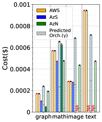
(a) All Workflows

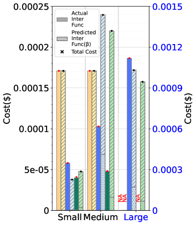
(b) Graph Workflow

Figure 17: Cost Analysis for Graph with different payload sizes, and for different workflows on medium payload size with static 1 RPS

For workflows with a large number of functions and edges AWS is costly, while for those with larger payloads, AzN and AzS are costly. AzN balances cost and performance.

The Graph workflow is the smallest of all, and we report the costs for running it on AWS, AzS and AzN in Fig. 17b for 1 RPS and all 3 payload sizes. AzN is the cheapest and AWS the costliest for all payloads, with AWS, AzS and AzN respectively costing $\mu\mathdollar 170$, $\mu\mathdollar 100$, and $\mu\mathdollar 48$. AzN is the cheapest due to the per hour throughput unit costing. This inter-function data transfer costs $(\beta)$ AzS is $250\%$ more than AzN. The total cost for AWS is also $252\%$ higher than AzN.

When we increase the payload size from small to medium, AWS has negligible increase in cost, by just $0.006\%$. The function execution time increase is small and its impact ($\alpha$) on the total cost is tiny. Changing the payload sizes does not impact the number of state transfers in AWS and hence does not change $\gamma$. For AzS, as we go from small to medium to large, the costs greatly increase from $\mu\mathdollar 58$ to $\mu\mathdollar 100$ to $\mu\mathdollar 1100$. The workflow orchestration costs increase the most small to large payload as it depends on the data volume and forms a large part of the total cost. For AzN, the costs are smaller but also increase substantially from $\mu\mathdollar 0.94$ to $\mu\mathdollar 48$ to $\mu\mathdollar 950$ (predicted) for similar reasons.

As the workflow becomes more complex with more functions and edges, AzN becomes costlier than AWS while AzS is the cheapest (Fig. 17a). For Math (15 funcs, 20 edges) and Image (9 funcs, 10 edges), AzN is $10.5\%$ and $53.5\%$ (predicted) costlier than AWS due to higher workflow orchestration costs caused by more accesses to the history table and data transfers. In contrast, AzS is $25.4\%$ and $163\%$ cheaper than AzN. AWS is the costliest for Text (25 funcs, 33 edges), having the most functions and edges. While AzS and AzN costs depend both on data transfers and state transitions across nodes and edges in the workflow, AWS is only affected by the latter. So more complex workflows are costlier for AWS while those with larger payloads costlier for Azure. AzN is cheaper for small and large workflows and yet offers performance comparable to AWS for non-intense workloads.

The bulk of the workflow execution cost is from the orchestration costs $\gamma$ for all three platforms.

The dominant cost is the workflow orchestration costs (Fig. 17a). These amount to $59\%$ to $92\%$ of the total costs for AzS and AzN, and over $99\%$ for AWS. The next highest for AzS and AzN is the inter-function data transfer costs at $8.5\%$ to $41\%$. Interestingly, the (predicted) function execution costs contribute the least, and stay well within the free tier. This means that the structure of the workflow (number of functions and edges) and payload sizes are the key cost factor for FaaS workflow, unlike for FaaS functions where the function execution costs dominate.

7 Discussions and Conclusions

In this article, we have performed a one-of-its-kind rigorous experimental study of three popular cloud FaaS workflow platforms from AWS and Azure. Our detailed suite of realistic workflows with diverse functions, composition patterns and workloads have been invoked for $\approx 132k$ workflow instances and $\approx 5.8M$ function calls across three data center regions to reveal unique performance and scalability insights which have not been explored elsewhere. Our key observations are backed up by a detailed analysis based on the experiments, micro-benchmarks and platform design. These expose the good (e.g., fast scaling on AWS, faster function execution on Azure), the bad (e.g., lack of large message size in AWS, high execution time variability for Azure) and the ugly (e.g., hardware heterogeneity within/across data centers, complex costing model of Azure).

Our observations offer practical benefits for developers, researchers and Cloud providers alike. Developers and be guided in the choice of CSP based on the scaling required for their workloads, workflow complexity, payload sizes, and cost management. While AWS offers several obvious advantages, its slower performance for function execution and higher cost for complex workflows offers Azure Netherite an edge. Researchers have the opportunity to design scheduling heuristics that leverage these insights, e.g., to automatically select the best CSP for a workflow and workload, selection of data centers, and even partitioning of the workflow across two CSPs [21]. Pre-warming strategies for workflows to avoid cascading cold-starts can also be explored. Lastly, Cloud Service Providers have the opportunity to fix some of their shortcomings, such as hardware heterogeneity and poor scaling causing high variability and non-deterministic SLAs for their customers, and complex and opaque pricing mechanisms.

Appendix A Appendix

A.1 Scaling with Input Rates

Fig. 18 reports the performance of Graph workflow with an increase in the maximum partition count (PC) on AzN, and complements Fig. 4 in the main article. This supports the analysis in § 6.1.

Fig. 19 reports additional plots for our experiments that could not fit within the main article. It shows the performance of the other workflows for 1 RPS and medium payload. This complements Fig. 5 in the main article that is focused on Graph workflow. It supports the analysis in § 6.1.1.

A.2 Cold Starts

A.2.1 Additional Plots on Coldstarts

The container cold-start latency is captured in the inter-function cold-start latency, as shown in Fig. 20. This expands upon Fig. 8 in the main article and supports 6.2.2. AzS and AzN load the entire workflow in memory when a coldstart occurs. So the expected behavior is that the Python runtime overhead should be constant across all the edges, but this is not what we observe. The inter-function latency also includes data transfer setup latency. Now this happens through Azure blobs for the medium size payload shown in the plot. The plot for small payload on Graph and Image (Figs. 20e and 20f) show that this coldstart overhead time is constant for small payloads ($\approx 4.1$s for graph and $\approx 5$s for image), i.e., when they are transferred via queues. This suggests that there is also some time that is required for setting up resources for Azure Blobs.

To confirm this we run an alternate experiment for the Graph workflow in which first three edges transfer data using queues (small payload) and last three via blobs (medium). We see in Fig. 20g that the cold start overheads (ColdStartTime minus WarmStartTime) for queue transfer edges are constant $\approx 1s$, while they vary for Blob transfer edges: $11.4s$, $8.4s$ and $19.6s$, respectively.

Fig. 21 shows the warmstart (yellow) and coldstart(blue) latencies for AzS and AzN on Graph and Image for medium payload, as discussed in 6.2.2. It complements Fig. 9 that is limited to AzN.

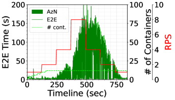
(a) Default, PC=12

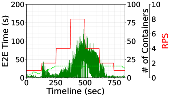
(b) PC=16

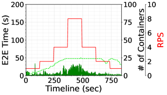
(c) PC=24

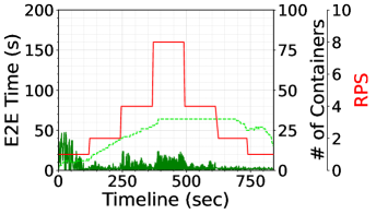
(d) Article, PC=32

Figure 18: AzN for Graph Workflow with Medium payload size and Step Workload, using different max. partition counts configurations.

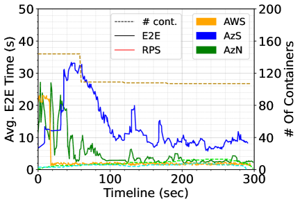
(a) Math Workflow | 1 RPS

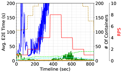
(b) Math Workflow | Step

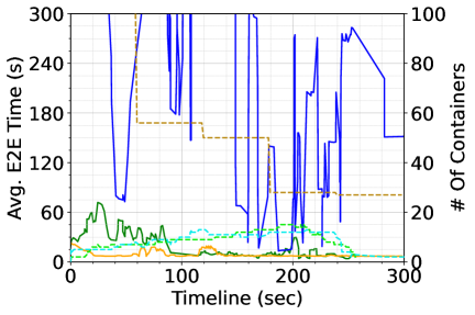
(c) Image Workflow | 1 RPS

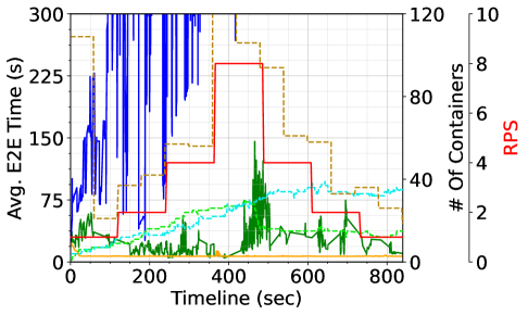
(d) Image Workflow | Step

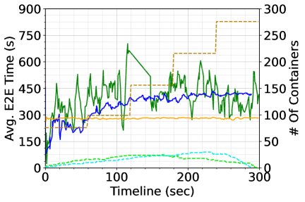
(e) Text Workflow | 1 RPS

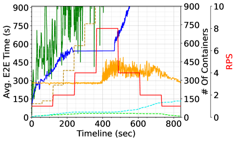
(f) Text Workflow | Step

Figure 19: Scaling of Math, Image and Text workflows with medium payload. Top row is for static 1 RPS workload while bottom row for Step workload.

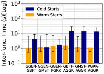
(a) AzS | Graph

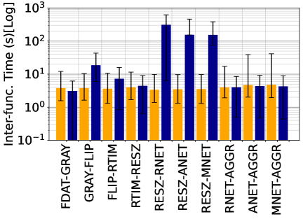
(b) AzS | Image

(c) AzN | Graph

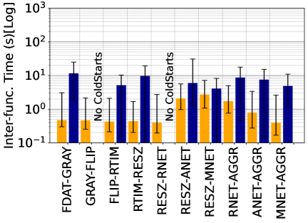
(d) AzN | Image

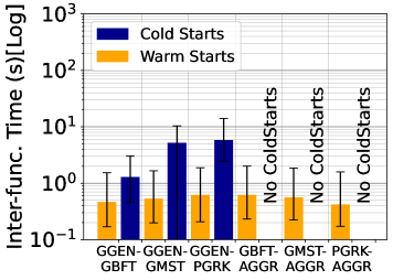
(e) AzS | Small | Graph

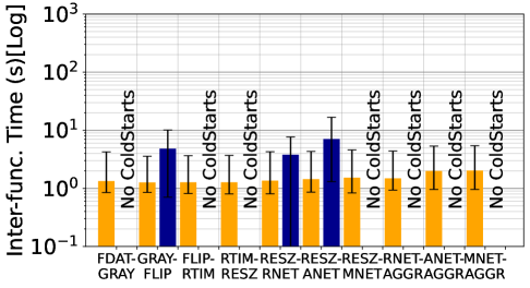
(f) AzS | Small | Image

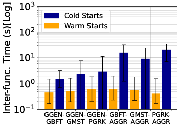
(g) AzS (Queue plus Blob transfers) | Graph

Figure 20: Inter-function latencies with and without container cold-starts for AzS and AzN, for Graph and Image workflows on medium payload and 1 RPS.

(a) Graph WF on AzS

(b) Graph WF on AzN

(c) Image WF on AzS

(d) Image WF on AzN

Figure 21: Function execution times with and without function cold-starts, for Graph and Image workflows with medium payload and static $1$ RPS

A.2.2 Estimating Container Coldstarts

As discussed in 6.2.2, whenever there is a cold-start in Azure, multiple steps take place. To accurately decompose the cold-start latency in Azure, we design a controlled micro-benchmark that isolates key overheads in function execution. The cold-start process consists of multiple sequential steps: (1) worker selection, (2) function application file system and settings mount, (3) runtime environment setup (e.g., Python, Node.js), (4) function loading into memory, and (5) function execution. The first three steps contribute to the container cold-start time ($t_{c}$), while the latter two steps together form the runtime cold-start time ($t_{r}$). Further, step (4) specifically corresponds to the inter-function cold-start overhead ($t_{i}$), which is influenced by the function package size $p$.

To quantify these values, we deploye a minimal workflow consisting of two empty functions that solely record execution time and container identifiers. No external imports were included to eliminate extraneous loading overheads ($t_{f}\approx 0$) and there is no other user logic. We execute this setup for three package sizes (50MB, 100MB, and 200MB) across AzS and AzN, measuring the total cold-start latency $T_{cp}$. Given the equation $t_{c}+t_{i}(p)+t_{f}=T_{cp}$, we estimate $t_{c}$ by regressing $T_{cp}$ against $p$, assuming a linear dependence of $t_{i}(p)$ on $p$. The resulting model yielded $t_{i}(p)\approx\alpha p+\beta$, where $\alpha$ and $\beta$ were empirically derived.

Our analysis reveals that $t_{c}\approx 290$ms for AzS and $t_{c}\approx 51.5$ms for AzN, accounting for approximately $40\%$ and $66.1\%$ of the total inter-function cold-start overhead, respectively. The difference in $t_{c}$ across environments aligns with the distinct scaling mechanisms in AzS and AzN, where AzS relies on a task hub with multiple storage services (queues, blobs, tables), whereas AzN scales through event hub partitions, effectively reducing initialization overhead. The high goodness-of-fit ($R^{2}=0.92$ for AzS and $R^{2}=0.99$ for AzN) supports the validity of our regression model in estimating $t_{i}(p)$ and isolating $t_{c}$.

A.3 Hardware Heterogeneity Plots for East USA and Central Europe

Fig. 22 provides additional plots here on the hardware heterogeneity and performance variability for different global data centers of Azure and AWS when running FaaS workflows. This complements Fig. 11 in the main article and supports 6.3.

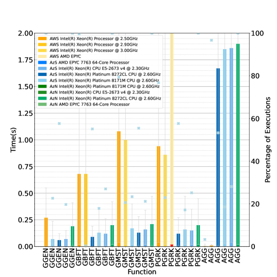
(a) East USA Graph

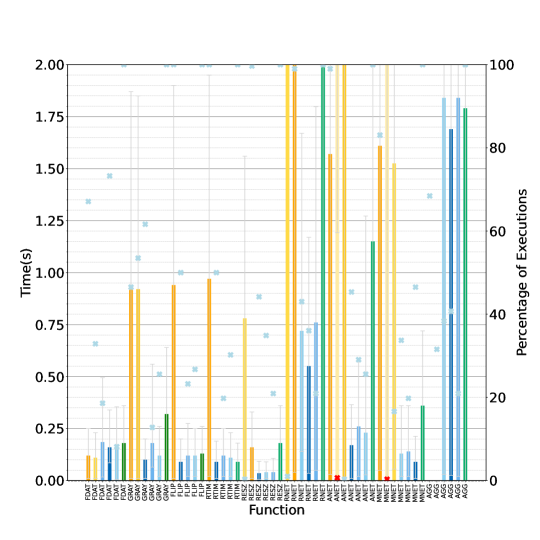
(b) East USA Image

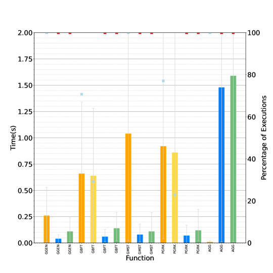
(c) Central Europe Graph

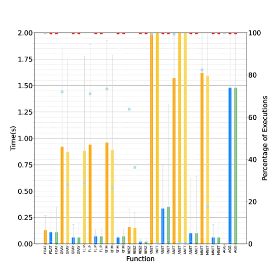
(d) Central Europe Image

Figure 22: Hardware Heterogeneity Across different Datacenters for Graph and Image workflow, medium payload , 1 RPS, 300s

References

- [1] G. C. Fox et al., “Status of serverless computing and function-as-a-service(faas) in industry and research,” CoRR, 2017.
- [2] M. Malawski, A. Gajek, A. Zima, B. Balis, and K. Figiela, “Serverless execution of scientific workflows: Experiments with hyperflow, aws lambda and google cloud functions,” Future Generation Computer Systems, 2020.
- [3] R. B. Roy, T. Patel, and D. Tiwari, “Daydream: Executing dynamic scientific workflows on serverless platforms with hot starts,” in International Conference on High Performance Computing, Networking, Storage and Analysis, 2022.
- [4] P. Leitner, E. Wittern, J. Spillner, and W. Hummer, “A mixed-method empirical study of function-as-a-service software development in industrial practice,” Journal of Systems and Software, 2019.
- [5] D. Chahal, S. C. Palepu, and R. Singhal, “Scalable and cost-effective serverless architecture for information extraction workflows,” in Workshop on High Performance Serverless Computing, 2022.
- [6] M. Shahrad et al., “Serverless in the wild: Characterizing and optimizing the serverless workload at a large cloud provider,” in USENIX Annual Technical Conference (ATC), 2020.
- [7] E. van Eyk, J. Scheuner, S. Eismann, C. L. Abad, and A. Iosup, “Beyond microbenchmarks: The spec-rg vision for a comprehensive serverless benchmark,” in Companion of the ACM/SPEC International Conference on Performance Engineering, 2020.
- [8] D. Barcelona-Pons and P. García-López, “Benchmarking parallelism in faas platforms,” Future Generation Computer Systems, 2021.
- [9] L. Wang, M. Li, Y. Zhang, T. Ristenpart, and M. Swift, “Peeking behind the curtains of serverless platforms,” in USENIX Annual Technical Conference (ATC), 2018.
- [10] P. Maissen, P. Felber, P. Kropf, and V. Schiavoni, “Faasdom: A benchmark suite for serverless computing,” in ACM International Conference on Distributed and Event-Based Systems, 2020.
- [11] J. Kim and K. Lee, “Functionbench: A suite of workloads for serverless cloud function service,” in 2019 IEEE 12th International Conference on Cloud Computing (CLOUD), 2019.
- [12] M. Copik et al., “Sebs: A serverless benchmark suite for function-as-a-service computing,” in International Middleware Conference, 2021.
- [13] J. Scheuner, R. Deng, J.-P. Steghöfer, and P. Leitner, “Crossfit: Fine-grained benchmarking of serverless application performance across cloud providers,” in IEEE/ACM International Conference on Utility and Cloud Computing (UCC), 2022.
- [14] H. Tian, S. Li, A. Wang, W. Wang, T. Wu, and H. Yang, “Owl: Performance-aware scheduling for resource-efficient function-as-a-service cloud,” in Symposium on Cloud Computing, 2022.
- [15] V. Kulkarni et al., “Xfbench: A cross-cloud benchmark suite for evaluating faas workflow platforms,” in IEEE International Symposium on Cluster, Cloud and Internet Computing (CCGrid), 2024.
- [16] S. Ginzburg and M. J. Freedman, “Serverless isn’t server-less: Measuring and exploiting resource variability on cloud faas platforms,” in International Workshop on Serverless Computing, 2021.
- [17] D. Ustiugov, T. Amariucai, and B. Grot, “Analyzing tail latency in serverless clouds with stellar,” in IEEE International Symposium on Workload Characterization (IISWC), 2021.
- [18] D. Ustiugov, P. Petrov, M. Kogias, E. Bugnion, and B. Grot, “Benchmarking, analysis, and optimization of serverless function snapshots,” in ACM International Conference on Architectural Support for Programming Languages and Operating Systems, 2021.
- [19] A. Tariq et al., “Sequoia: Enabling quality-of-service in serverless computing,” in ACM Symposium on Cloud Computing, 2020.
- [20] S. Burckhardt et al., “Netherite: Efficient execution of serverless workflows,” Proc. VLDB Endow., 2022.
- [21] A. Khochare, T. Khare, V. Kulkarni, and Y. Simmhan, “Xfaas: Cross-platform orchestration of faas workflows on hybrid clouds,” in IEEE/ACM International Symposium on Cluster, Cloud and Internet Computing (CCGrid), 2023.
- [22] J. Li et al., “Analyzing open-source serverless platforms: Characteristics and performance,” CoRR, vol. abs/2106.03601, 2021.
- [23] J. Wen et al., “Characterizing commodity serverless computing platforms,” Journal of Software: Evolution and Process, 2023.
- [24] P. Garcia Lopez, M. Sanchez-Artigas, G. Paris, D. Barcelona Pons, A. Ruiz Ollobarren, and D. Arroyo Pinto, “Comparison of faas orchestration systems,” in 2018 IEEE/ACM International Conference on Utility and Cloud Computing Companion (UCC Companion), 2018.
- [25] N. Shahidi, J. R. Gunasekaran, and M. T. Kandemir, “Cross-platform performance evaluation of stateful serverless workflows,” in IEEE International Symposium on Workload Characterization (IISWC), 2021.
- [26] T. Yu, Q. Liu, D. Du, Y. Xia, B. Zang, Z. Lu, P. Yang, C. Qin, and H. Chen, “Characterizing serverless platforms with serverlessbench,” in ACM Symposium on Cloud Computing, 2020.
- [27] S. Ristov, C. Hollaus, and M. Hautz, “Colder than the warm start and warmer than the cold start! experience the spawn start in faas providers,” 2022.
- [28] R. Wang, G. Casale, and A. Filieri, “Enhancing performance modeling of serverless functions via static analysis,” in International Conference on Service-Oriented Computing (ICSOC), 2022.
- [29] J. Wen and Y. Liu, “An empirical study on serverless workflow service,” arXiv, no. 2101.03513, 2021.
- [30] C. Lin and H. Khazaei, “Modeling and optimization of performance and cost of serverless applications,” IEEE Transactions on Parallel and Distributed Systems, 2021.
- [31] J. Wen and Y. Liu, “A measurement study on serverless workflow services,” in 2021 IEEE International Conference on Web Services (ICWS), 2021.
- [32] S. Eismann, J. Grohmann, E. van Eyk, N. Herbst, and S. Kounev, “Predicting the costs of serverless workflows,” in ACM/SPEC International Conference on Performance Engineering, 2020.
- [33] A. Mahgoub et al., “Wisefuse: Workload characterization and dag transformation for serverless workflows,” Proc. ACM Meas. Anal. Comput. Syst., 2022.
- [34] J. Scheuner and P. Leitner, “Function-as-a-service performance evaluation: A multivocal literature review,” Journal of Systems and Software, 2020.
- [35] M. Grambow, T. Pfandzelter, L. Burchard, C. Schubert, M. Zhao, and D. Bermbach, “Befaas: An application-centric benchmarking framework for faas environments,” in IEEE International Conference on Cloud Engineering (IC2E 2021), 2021.
- [36] Gan et al., “An open-source benchmark suite for microservices and their hardware-software implications for cloud & edge systems,” in International Conference on Architectural Support for Programming Languages and Operating Systems, 2019.
- [37] Z. Li et al., “Help rather than recycle: Alleviating cold startup in serverless computing through Inter-Function container sharing,” in USENIX Annual Technical Conference (ATC), 2022.
- [38] P. Silva, D. Fireman, and T. E. Pereira, “Prebaking functions to warm the serverless cold start,” in International Middleware Conference, 2020.
- [39] A. Kumari and B. Sahoo, “Acpm: adaptive container provisioning model to mitigate serverless cold-start,” Cluster Computing, 2023.
- [40] B. Wang, A. Ali-Eldin, and P. Shenoy, “Lass: Running latency sensitive serverless computations at the edge,” in International Symposium on High-Performance Parallel and Distributed Computing, 2021.
- [41] S. Kotni, A. Nayak, V. Ganapathy, and A. Basu, “Faastlane: Accelerating Function-as-a-Service workflows,” in USENIX Annual Technical Conference (ATC), 2021.
- [42] V. Sreekanti, C. Wu, X. C. Lin, J. Schleier-Smith, J. E. Gonzalez, J. M. Hellerstein, and A. Tumanov, “Cloudburst: stateful functions-as-a-service,” Proc. VLDB Endow., 2020.
- [43] Z. Jia and E. Witchel, “Nightcore: efficient and scalable serverless computing for latency-sensitive, interactive microservices,” in ACM International Conference on Architectural Support for Programming Languages and Operating Systems, 2021.
- [44] S. Burckhardt, B. Chandramouli, C. Gillum, D. Justo, K. Kallas, C. McMahon, C. S. Meiklejohn, and X. Zhu, “Netherite: efficient execution of serverless workflows,” Proc. VLDB Endow., 2022.
- [45] M. Brooker et al., “On-demand container loading in AWS lambda,” in 2023 USENIX Annual Technical Conference (USENIX ATC 23), 2023.
- [46] S. Luo, H. Xu, C. Lu, K. Ye, G. Xu, L. Zhang, Y. Ding, J. He, and C. Xu, “Characterizing microservice dependency and performance: Alibaba trace analysis,” in ACM Symposium on Cloud Computing, 2021.
- [47] P. S. Vinayak, S. S. Mallick, L. Jagarlamudi, A. Chakraborty, and Y. Simmhan, “CARL: cost-optimized online container placement on vms using adversarial reinforcement learning,” IEEE Trans. Cloud Comput., vol. 13, no. 1, pp. 321–335, 2025.
- [48] A. Shukla, S. Chaturvedi, and Y. Simmhan, “Riotbench: An iot benchmark for distributed stream processing systems,” Concurrency and Computation: Practice and Experience, 2017.
- [49] L. Lu, P. J. Varman, and K. Doshi, “Decomposing workload bursts for efficient storage resource management,” IEEE Transactions on Parallel and Distributed Systems, 2011.
- [50] A. Agache, M. Brooker, A. Florescu, A. Iordache, A. Liguori, R. Neugebauer, P. Piwonka, and D.-M. Popa, “Firecracker: Lightweight virtualization for serverless applications,” in NSDI, 2020.
- [51] A. Wang et al., “Faasnet: Scalable and fast provisioning of custom serverless container runtimes at alibaba cloud function compute,” in USENIX Annual Technical Conference (ATC), 2021.