MoE-PHDS: One MoE checkpoint for flexible runtime sparsity

Abstract

Sparse Mixtures of Experts (MoEs) are typically trained to operate at a fixed sparsity level, e.g. $k$ in a top-$k$ gating function. This global sparsity level determines an operating point on the accuracy/latency curve; currently, meeting multiple efficiency targets means training and maintaining multiple models. This practice complicates serving, increases training and maintenance costs, and limits flexibility in meeting diverse latency, efficiency, and energy requirements. We show that pretrained MoEs are more robust to runtime sparsity shifts than commonly assumed, and introduce MoE-PHDS (Post Hoc Declared Sparsity), a lightweight SFT method that turns a single checkpoint into a global sparsity control surface. PHDS mixes training across sparsity levels and anchors with a short curriculum at high sparsity, requiring no architectural changes. The result is predictable accuracy/latency tradeoffs from one model: practitioners can “dial $k$” at inference time without swapping checkpoints, changing architecture, or relying on token-level heuristics. Experiments on OLMoE-1B-7B-0125, Qwen1.5-MoE-A2.7B, and proprietary models fit on multiple operating points show that PHDS matches or exceeds well-specified oracle models, improves cross-sparsity agreement by up to 22% vs. well-specified oracle models, and enables simplified, flexible runtime MoE deployment by making global sparsity a first-class serving primitive.

1 Introduction

Mixture of Experts (MoEs) language models deliver state-of-the-art quality with lower active compute by routing tokens through a subset of active experts per layer (Liu et al., 2024; Du et al., 2022). At deployment, sparsity level (e.g. $k$ in top-$k$) is fixed, so supporting multiple operating points has required multiple checkpoints. We argue this is not necessary. First, pretrained MoEs already tolerate moderate runtime sparsity shifts. Second, with MoE-PHDS we make this tolerance more predictable: a short SFT schedule across sparsity levels with curriculum anchoring produces a single checkpoint reusable at different sparsity levels. This enables more predictable accuracy/latency tradeoffs, SLA-aware serving, and energy-aware throttling from one model.

Prior work, like adaptive routing(Huang et al., 2024; Nishu et al., 2025; Alizadeh-Vahid et al., 2024) and null experts (Zeng et al., 2024; Yan et al., 2025; Team et al., 2025), focuses on token-level choices. These can spend a fixed global budget more efficiently, but add variance (latency depends on input) and policy complexity (extra knobs). In contrast, PHDS exposes one global knob: $k$, which yields more predictable accuracy/latency tradeoffs. This simplicity is key for deployment.

Prior work in adaptive computation, such as slimmable networks (Yu et al., 2019), Once-for-All models (Cai et al., 2020), MatFormer (Devvrit et al., 2024), and Flextron (Cai et al., 2024), demonstrates that dense networks can support multiple operating points from a single model. In contrast, the prevailing approach is that each global MoE sparsity level needs its own checkpoint, often from a separate pretraining run. This practice of supporting only well-specified models leads to training and storing multiple models, and has stymied study about model behavior when inference sparsity is not well-specified. As such, fundamental questions remain unanswered: Can a single MoE checkpoint generalize across multiple global levels of sparsity? What mechanisms block or enhance model flexibility?

Our work challenges the fixed-sparsity assumption. We show that MoEs are robust to small-to-moderate changes in the global sparsity parameter. Empirically, we show that flexibility can be supported by a single checkpoint. For example, we show that for OLMoE-1B-7B-0125, reducing $k$ at runtime from 8 to 6 decreases multiple choice accuracy by 1.2% (relative) and increases wikitext perplexity by 6.4%; likewise, for Qwen1.5-MoE-A2.7B, reducing $k$ from 4 to 3 results in only a 0.43% accuracy reduction and 1.2% perplexity increase. These findings highlight an overlooked generalization property, with direct implications for efficiency-constrained AI deployment.

Building on this observation, we introduce a lightweight supervised fine tuning (SFT) method to reliably and stably produce models for cross-sparsity deployment. Rather than requiring different checkpoints for different sparsity levels, our proposed method, a Mixture of Experts with Post Hoc Declared Sparsity (MoE-PHDS), produces a single checkpoint for use across sparsity levels. See figure 1 for an overview and figure 2 for a comparison with current practice. On public models, our method matches or exceeds baselines, and shows benefits, such as higher accuracy and support for extended sparsity ranges, on internal models.

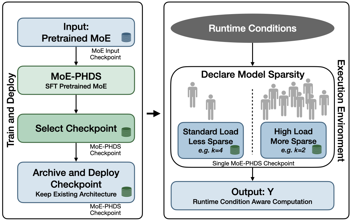
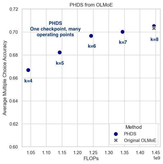
Figure 1: Overview of our proposed framework, MoE-PHDS. The left represents how a robust, sparsity-flexible single checkpoint is generated. The center shows how the model is called under dynamic runtime conditions. The right panel shows average multiple choice task accuracy vs. flops with 4096 context length using OLMoE-1B-7B-0125 as a base pretrain model, along with the a well-specified model. There is little accuracy degradation as $k$ is reduced from 8 to 6.

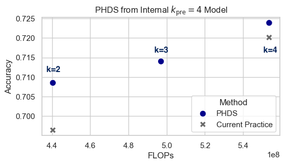
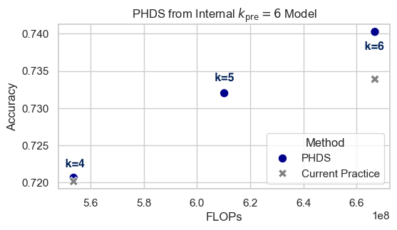
Figure 2: FLOPs vs. average multiple choice accuracy for internal models trained at the current practice (multiple checkpoints for each $k$) (crosses) and PHDS models (dots); all methods are SFTed on CommonSense170k. Left: two internal models trained at $k=2$ and $k=4$ vs. a single PHDS checkpoint, evaluated at $k=\{2,3,4\}$. Right: two internal models trained at $k=4$ and $k=6$ vs. a single PHDS checkpoint, evaluated at $k=\{4,5,6\}$. PHDS reduced training by 50% compared to current practice and offered support on a wider range of $k$ for each setting.

Inference-time sparsity mis-specification can be viewed as a feature of MoE models rather than a bug. Classical mis-specification is when a data-generating regime is not supported by a model class, such as using a linear model for data with a non-linear relationship. Here we study an MoE deployment variant: at inference time we intentionally restrict the model space (fewer experts than used in pretraining), by declaring a smaller $k$ after training. PHDS makes this intentional restriction better supported by introducing the model to various $k$ levels during SFT, we keep predictions stable when $k$ is set at runtime. Practically, this yields (i) controllability, since a single parameter governs global sparsity, and (ii) predictability with respect to changes in FLOPS or accuracy. In short, we turn “mis-specification” into a serving primitive to produce predictable resource-quality tradeoffs.

From an operational standpoint, global control of sparsity at runtime unlocks capabilities that fixed-sparsity or token-level sparsity models do not have. First, it enables service level agreement (SLA)-aware serving, where a model can adjust sparsity based on user tier, request type, latency budget, or system load. This can mitigate latency spikes and promote tenant fairness without swapping models. Additionally, explicit, discrete $k$ selection per query allows predictable accuracy/latency tradeoffs compared to token-level sparsity. Second, it enables energy-aware inference: sparser models can be used during system wide energy constraints and scale to full model size when resources are not constrained. Finally, it offers substantial operational simplicity: rather than managing a fleet of sparsity-specific models with separate pipelines, drift risks and possibly architectures, practitioners can deploy a single, flexible checkpoint. We focus on small to moderately size models (1B-14.3B), where deployment memory and energy budgets are often the tightest. This paper makes the following contributions:

• Sparsity level as a serving primitive. We show that pretrained MoEs tolerate moderate runtime sparsity shifts with minimal loss, challenging the assumption that each sparsity level requires its own checkpoint, allowing sparsity level to act as a serving primitive.

• MoE-PHDS method. We propose a lightweight SFT recipe—multi-$k$ training with curriculum anchoring—that enables a single checkpoint to operate flexibly across sparsity levels.

• Deployment benefits. We demonstrate that PHDS improves cross-sparsity output agreement (7–22%), yielding stable user-facing behavior while reducing operational complexity: one checkpoint, one control surface, and predictable tradeoffs.

2 MoE-PHDS Framework

We introduce an SFT method that allows a pretrained MoE model to support runtime-declared sparsity levels. MoE-PHDS consists of two phases: (1) Multi-$k$ Training, in which the model is fine-tuned by randomly varying the number of active experts $k$ across forward passes, and (2) Curriculum Anchoring, in which training is annealed to a lower $k$ to stabilize expert routing. Once fine-tuned, a single checkpoint can be deployed and reused across a range of sparsity levels. Let $k_{\mathrm{pre}}$ be the sparsity level from the pretrained model, $k_{\mathrm{train},\,i}$ the sparsity for forward pass iteration $i$, and $k_{\mathrm{ev}}$ is the evaluation sparsity level. Since expert parameters are only pretrained up to $k_{\mathrm{pre}}$, we restrict training and evaluation to $k_{\mathrm{train},i},k_{\mathrm{ev}}\leq k_{\mathrm{pre}}$.

2.1 Multi-$k$ Training

The goal of Multi-$k$ Training is to expose the model to a range of sparsity levels so that it can generalize beyond fixed $k_{\mathrm{pre}}$. We define a set of candidate sparsity levels, $\mathcal{K}_{\mathrm{train}}\subset\mathbb{N}$ (e.g. $\{4,5,6,7,8\}$). For each forward pass $i$, we uniformly sample $k_{train,\,i}$ from $\mathcal{K}_{\mathrm{train}}$ and compute the language modeling loss, such as cross-entropy, under this sparsity. Any auxiliary components (e.g., load-balancing losses, layer norms) are stored and updated per $k$. In practice, we observe rapid convergence, especially when the fine-tuning dataset is distributionally aligned with pretraining data.

2.2 Curriculum Anchoring

Although Multi-$k$ Training improves robustness across multiple $k$, performance can degrade at very low $k$ due to interference from higher-$k$ co-activation patterns. To address this, we introduce Curriculum Anchoring: after an initial phase of Multi-$k$ Training, we gradually anneal training toward a fixed, lower $k_{\mathrm{train}}$ (e.g., $k=2$). This stabilizes expert dynamics at sparse settings and improves reliability when $k_{\mathrm{ev}}\ll k_{\mathrm{pre}}$.

2.3 Implementation Details

Pretrained MoE models are not typically designed for runtime sparsity variation. MoE-PHDS introduces minimal modifications to support this flexibility. Let $h\in\mathbb{R}^{d}$ denote the hidden state, $W_{r}\in\mathbb{R}^{d\times E}$ the router weights, and $E$ the number of experts. Router logits are $z=W_{r}h$, with $p=\mathrm{softmax}(z;k_{\mathrm{pre}})$ the raw gating probabilities. We use a soft mask to adapt $p$ to different $k_{\mathrm{train}}$:

$$p_{j}=\begin{cases}p_{j}&\text{if }j\in\mathrm{top\text{-}k_{\mathrm{train},i}}(p),\\ \epsilon&\text{if }j\in\mathrm{top\text{-}k_{\mathrm{pre}}}(p)\setminus\mathrm{top\text{-}k_{\mathrm{train},i}}(p),\\ 0&\text{otherwise,}\end{cases}$$ (1)

$\epsilon$ is a tunable parameter, we use 1E-6. For unnormalized top-$k$-softmax routers, equation 1 remains unnormalized; for normalized $\text{softmax-}k$ routers, the masked probabilities are renormalized. Layer norm parameters and load balancing loss, if applicable, need to be stored and activated by $k_{\mathrm{train}}$.

Checkpoint Selection.

Multi-$k$ Training with Curriculum Anchoring produces a family of candidate checkpoints. A single checkpoint is chosen after anchoring, either by best validation performance at a target $k_{\mathrm{ev}}$ or by average performance across a range of $k_{\mathrm{ev}}$. We use values at $k_{\mathrm{pre}}$ since we assume it is the default operating point. At runtime, operators declare the desired sparsity level, and the same checkpoint can be reused without retraining.

3 Experiments

Our experiments test whether one checkpoint can support multiple runtime sparsity levels and when PHDS outperforms oracle or naive baselines. PHDS fine-tuning adds a fraction of pretraining cost, since it is a short SFT pass reusing existing checkpoints. Broadly, public well-tuned models (OLMoE, Qwen) are already robust to modest sparsity shifts, while less tuned internal models show consistent gains from PHDS. Across models, PHDS maintains $\leq$1–2% relative QA drop when $k$ is reduced by up to 25% (e.g., OLMoE: $k=$8→6, Qwen:$k=$4→3). Below $k_{\mathrm{pre}}/2$, degradation becomes more pronounced.

3.1 Experimental Setup

3.1.1 Pretrained Models and Fine-tune Data

Table 1: Summary of Pretrained Models

Model	$k_{\mathrm{pre}}$	Experts	Active Params	Total Params	SFT
Internal-Baseline-2	2	16	240M	1.032B	No
Internal-Baseline-4	4	16	353M	1.032B	No
Internal-Baseline-6	6	16	466M	1.032B	No
OLMoE-1B-7B-0125	8	64	1B	7B	No
OLMoE-1B-7B-0125-Instruct	8	64	1B	7B	Yes
Qwen1.5-MoE-A2.7B	4	60	2.7B	14.3B	No
Qwen1.5-MoE-A2.7B-Chat	4	60	2.7B	14.3B	Yes

Internal Baseline Model.

We pretrain three MoEs (24 layers; model dim 1024; FFN dim 12,288; 16 experts/layer; 1.032B total params) with $k_{\mathrm{pre}}\in\{2,4,6\}$ and softmax–top-$k$ routers. See table 1 for pretrained model specifications.

OLMoE.

We evaluate OLMoE-1B-7B-0125 and its instruction-tuned variant (Muennighoff et al., 2024). Both use 8/64 experts per layer with a top-$k$–softmax router.

Qwen.

We evaluate Qwen1.5-MoE-A2.7B and the chat-tuned variant (Qwen Team, 2024), which use 4/60 experts per layer with a top-$k$–softmax router.

Fine-Tuning Data.

We use CommonSense170K from LLM-Adapters (Hu et al., 2023), the tulu3-sft-olmo-2-mixture dataset (Lambert et al., 2024), and a high-quality internal mixture (“Internal Baseline Data Set” comprised of licensed; curated public/open data; and a web crawled subset) for additional SFT.

3.1.2 Fine-tuning Regimes

Prior work on MoE flexibility focuses on token-level adaptability given a fixed global sparsity budget or uses architectural changes. We are interested in MoE robustness to train/inference mis-specification for a fixed architecture. Hence, we use well-specified oracle models as a baseline and compare a set of fine tuning regimes.

Oracle.

Fine-tune at $k_{\mathrm{pre}}$; denoted $\text{Oracle }k_{\mathrm{pre}}$; evaluated at any $k_{\mathrm{ev}}$. This is a well-specified baseline when evaluated at $k_{\mathrm{ev}}=k_{\mathrm{pre}}$.

Naive.

Fine-tuned at a single, lower $k_{\mathrm{train}}<k_{\mathrm{pre}}$; denoted $k_{\mathrm{pre}}\!\rightarrow\!k_{\mathrm{train}}$, e.g. $4\!\rightarrow\!2$.

MoE-PHDS.

Sample $k$ uniformly from $\mathcal{K}_{\mathrm{train}}$ during SFT, optionally anneal to a low anchor $k_{\mathrm{train}}$; denoted $\mathcal{K}_{\mathrm{train}}\!\rightarrow k_{\mathrm{train}}$, e.g., $[2,3,4]\!\rightarrow\!2$ or $[2,3,4]$ for a non-curriculum trained variant.

3.1.3 Selection and Evaluation Protocol

Unless otherwise noted, we select the checkpoint with the best multiple-choice QA accuracy at $k_{\mathrm{ev}}=k_{\mathrm{pre}}$ after a 5,000-step burn-in as pretrain model-task misalignment may cause accuracy decreases. Public models use tulu3-sft-olmo-2-mixture (Tülu-3) for SFT; internal models use the Internal Baseline Data Set or CommonSense170K. All regimes are SFTed with the same settings per ablation. We evaluate with lm-evaluation-harness for zero shot multiple choice QA: ARC Challenge and Easy (Clark et al., 2018), BoolQ (Clark et al., 2019), HellaSwag (Zellers et al., 2019), PIQA (Bisk et al., 2020), SciQ (Welbl et al., 2017), and Winogrande (Sakaguchi et al., 2021); TriviaQA-fixed (Joshi et al., 2017) for generative QA; and WikiText (Merity et al., 2016) perplexity. For CommonSense170K on Internal Baseline Models, we follow LLM-Adapters’ stricter matching protocol and evaluate on their multiple choice QA set: ARC-C/E, BoolQ, PIQA, HellaSwag, Winogrande, SocialIQA (Sap et al., 2019), and Openbook QA (Mihaylov et al., 2018). All methods are evaluated at a single checkpoint. For all tables, best results are in bold, second-best underlined; well-specified models are in blue.

3.2 Internal Baselines: CommonSense170K

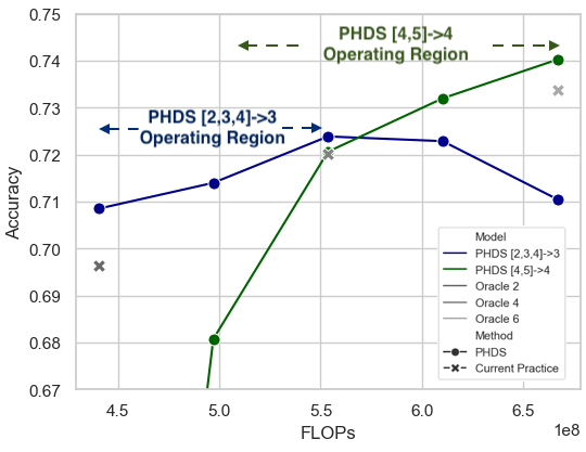
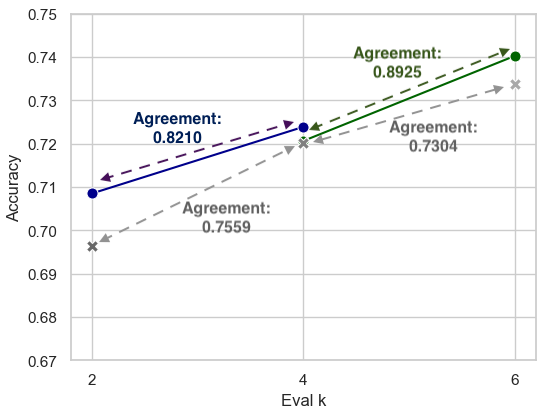
Figure 3: (Left) Average accuracy vs. flops with 4096 context length for Internal Baseline Models. Current practice (Oracle models operating at $k_{\mathrm{pre}}$; denoted by crosses) is compared with PHDS (dots), which produces a range of operating points PHDS operating regions are based on pretrained models, but show ability to meet or outperform baseline models with reduced training costs. (Right) Average accuracy vs. $k_{\mathrm{ev}}$, with answer agreement between checkpoints. Despite similar accuracy, PHDS has increased agreement compared to current practice.

We fine-tune untuned Internal Baseline Models on CommonSense170K to study (1) accuracy under evaluation sparsity mis-specification, (2) sensitivity of MoE-PHDS to $\mathcal{K}_{\mathrm{train}}$ and curricula, and (3) cross-$k$ agreement. We begin curriculum after 10,000 steps ($\approx$93.9% of epoch 1). Evaluation uses strict matching on 1,000 samples per task. Figure 3 highlights the difference between PHDS and current methods: using Oracle models at $k_{\mathrm{pre}}$, forcing practitioners to maintain multiple models. In contrast, a single PHDS checkpoint spans multiple sparsity levels, while maintaining accuracy close to or above Oracle at its $k_{\mathrm{pre}}$. Full results are in table 2. We find that all families (Oracle/Naive/PHDS) tolerate modest decreases in $k_{\mathrm{ev}}$ with limited accuracy loss; increasing beyond $k_{\mathrm{pre}}$ does not recover denser-oracle performance. Evaluating below $k_{\mathrm{pre}}/2$ produces poor results. PHDS often matches or slightly exceeds the corresponding Oracle around $k_{\mathrm{pre}}$, while producing superior results for mis-specified models.

Table 2: CommonSense170K SFT: overall accuracy (average across tasks).

Model	$k_{\mathrm{pre}}$	$k_{\mathrm{ev}}{=}2$	$k_{\mathrm{ev}}{=}3$	$k_{\mathrm{ev}}{=}4$	$k_{\mathrm{ev}}{=}5$	$k_{\mathrm{ev}}{=}6$
Oracle 2	2	0.69638	0.66750	0.70025	0.05750	0.00013
Oracle 4	4	0.66113	0.70663	0.72013	0.72688	0.71025
PHDS $k{=}[2,3,4]\!\rightarrow\!3$	4	0.70850	0.71400	0.72388	0.72288	0.71050
Naive $4\!\rightarrow\!2$	4	0.69850	0.71863	0.70488	0.56913	0.21150
Oracle 6	6	0.44350	0.66013	0.72200	0.73163	0.73388
PHDS $k{=}[4,5]\!\rightarrow\!4$	6	0.47800	0.68075	0.72063	0.73200	0.74025
Naive $6\!\rightarrow\!4$	6	0.48275	0.68175	0.72275	0.72788	0.73025

For operators to vary sparsity at runtime without altering user experience, outputs should remain consistent across $k_{\mathrm{ev}}$. We quantify agreement between two models $M_{1},M_{2}$ by averaging discrete answer, $M_{j,i}$, equality over items $i$: $\mathcal{A}(M_{1},M_{2})=\frac{1}{N}\sum_{i=1}^{N}\mathbf{1}\{M_{1,i}=M_{2,i}\}.$ We compare answer agreement of two separate well-specified models with different checkpoints vs. a single PHDS checkpoint evaluated at different sparsity levels in figure 3. Across both $(2,4)$ and $(4,6)$ comparisons, a single PHDS checkpoint yields $7\%{-}22\%$ higher cross-$k$ agreement than using two separate well-specified Oracle checkpoints, at similar accuracy levels.

3.2.1 Internal Baseline Model: Internal Data Mixture

Here we SFT the Internal Baseline models on a subset of the Internal Data Mixture to measure responsiveness to fine-tuning under mis-specification. Oracle models change little from the pretrained models, while Naive and PHDS shift their performance profiles. Internal models use $k_{\mathrm{pre}}\in\{2,4,6\}$. From $k_{\mathrm{pre}}{=}4$: PHDS $[2,3,4]\!\rightarrow\!3$ and Naive $4\!\rightarrow\!2$. From $k_{\mathrm{pre}}{=}6$: PHDS $[4,5]\!\rightarrow\!4$ and Naive $6\!\rightarrow\!4$. We report multiple-choice QA averages, TriviaQA-fixed (generative QA), and WikiText perplexity (table 3). We find that PHDS is broadly competitive. Across $k_{\mathrm{ev}}\in\{2,3,4,5,6\}$, PHDS is typically within $1\!\sim\!2\%$ of the best Oracle for well-specified $k_{\mathrm{ev}}$, and often second-best across settings. For generative QA and perplexity, trends mirror QA accuracy: PHDS and Naive are competitive at their target $k$, with Oracle best at its native $k$; PHDS avoids steep degradations when $k_{\mathrm{ev}}$ shifts.

Table 3: Internal Baselines fine-tuned on the Internal Baseline Data Set. Models are grouped by $k_{\mathrm{pre}}$ and $k_{\mathrm{ev}}$.

Method	ARC-C	ARC-E	boolq	hella	piqa	sciq	wino	Avg	triv	wiki
$k_{\mathrm{ev}}=2$
Oracle 2	0.3242	0.6650	0.6291	0.4464	0.7323	0.899	0.5912	0.6125	0.0813	14.039
Oracle 4	0.2944	0.5867	0.5000	0.4235	0.7155	0.844	0.5406	0.5578	0.0243	20.800
[2,3,4]→3	0.2833	0.6284	0.5654	0.4302	0.7329	0.882	0.5533	0.5822	0.0351	16.274
4→2	0.2952	0.6402	0.5966	0.4379	0.7263	0.892	0.5943	0.5975	0.0480	15.088
$k_{\mathrm{ev}}=3$
Oracle 4	0.3250	0.6599	0.6174	0.4613	0.7459	0.901	0.5959	0.6157	0.0522	14.184
[2,3,4]→3	0.3251	0.6734	0.6302	0.4522	0.7448	0.914	0.6030	0.6204	0.0555	13.933
4→2	0.3174	0.6591	0.6398	0.4369	0.7285	0.906	0.5927	0.6115	0.0480	14.889
Oracle 6	0.2696	0.5749	0.5232	0.4226	0.6882	0.799	0.5351	0.5447	0.0269	26.144
[4,5]→4	0.2858	0.6141	0.5746	0.4376	0.7133	0.851	0.5525	0.5755	0.0366	16.848
6→4	0.2969	0.6178	0.5780	0.4408	0.7160	0.857	0.5446	0.5787	0.0442	16.762
$k_{\mathrm{ev}}=4$
Oracle 4	0.3430	0.6772	0.6388	0.4654	0.7465	0.910	0.6109	0.6274	0.0556	13.355
[2,3,4]→3	0.3353	0.6776	0.6440	0.4587	0.7443	0.910	0.6054	0.6250	0.0611	13.564
4→2	0.3038	0.6595	0.6514	0.4242	0.7171	0.909	0.5991	0.6091	0.0441	15.972
Oracle 6	0.3106	0.6460	0.5841	0.4633	0.7252	0.867	0.5951	0.5988	0.0617	15.688
[4,5]→4	0.3012	0.6670	0.6171	0.4609	0.7350	0.886	0.5967	0.6077	0.0591	14.024
6→4	0.3114	0.6557	0.6294	0.4587	0.7367	0.887	0.6101	0.6127	0.0636	13.955
$k_{\mathrm{ev}}=5$
Oracle 6	0.3379	0.6662	0.6205	0.4772	0.7432	0.892	0.6069	0.6206	0.0769	13.494
[4,5]→4	0.3328	0.6751	0.6443	0.4680	0.7405	0.893	0.6085	0.6232	0.0729	13.303
6→4	0.3234	0.6709	0.6443	0.4592	0.7345	0.898	0.6062	0.6195	0.0681	13.746
$k_{\mathrm{ev}}=6$
Oracle 6	0.3353	0.6793	0.6269	0.4761	0.7416	0.899	0.6148	0.6247	0.0751	13.092
[4,5]→4	0.3259	0.6806	0.6382	0.4665	0.7405	0.900	0.6062	0.6226	0.0673	13.224
6→4	0.3063	0.6667	0.6413	0.4508	0.7334	0.902	0.6046	0.6150	0.0605	14.219

3.3 OLMoE

We assess mis-specification on OLMoE-1B-7B-0125 with SFT on Tülu-3. We compare $\text{Oracle }k{=}8$, $\text{PHDS }[4,5,6,7,8]\!\rightarrow\!5$, $\text{PHDS }[4,5,6,7,8]$, and $\text{Naive }8\!\rightarrow\!4$. Results for average multiple choice (Avg), TriviaQA (triv), and wikitext perplexity (wiki) are in table 4; full results by task are in the Appendix in section A.4. We find that: (i) all SFT methods are similar, and () robustness to sparsity. At $k_{\mathrm{ev}}\in\{8,7,6,5,4\}$, both accuracy and perplexity remain close across methods. For the base OLMoE model, perplexity stays within $\sim$1.5–6.4% of the well-specified model for $k_{\mathrm{ev}}\in\{6,7,8\}$, with overall relative accuracy differences $\leq 1.5\%$.

Table 4: OLMoE fine-tuned on Tülu-3.

		OLMoE-1B-7B-0125			OLMoE-0125-1B-7B-Instruct
Method	$k_{\mathrm{ev}}$	Avg	triv	wiki	Avg	triv	wiki
Oracle	8	0.7050	0.4889	9.407	0.7067	0.3977	15.810
[4,5,6,7,8]→5	8	0.6997	0.4585	8.923	0.7068	0.4131	15.742
[4,5,6,7,8]	8	0.7051	0.4901	8.903	0.7041	0.4119	15.484
8→4	8	0.7021	0.4794	9.485	0.7059	0.4174	15.488
Oracle	7	0.7017	0.4928	9.557	0.7022	0.3902	16.238
[4,5,6,7,8]→5	7	0.6939	0.4578	9.075	0.7006	0.3928	16.280
[4,5,6,7,8]	7	0.7001	0.4815	9.056	0.6999	0.3973	16.014
8→4	7	0.6966	0.4793	9.639	0.7008	0.4003	16.042
Oracle	6	0.6967	0.4817	9.985	0.6953	0.3756	17.372
[4,5,6,7,8]→5	6	0.6893	0.4667	9.496	0.6934	0.3842	17.426
[4,5,6,7,8]	6	0.6966	0.4767	9.474	0.6906	0.3862	17.148
8→4	6	0.6924	0.4737	10.091	0.6943	0.3909	17.188
Oracle	5	0.6849	0.4487	10.975	0.6837	0.3686	19.687
[4,5,6,7,8]→5	5	0.6742	0.4242	10.431	0.6831	0.3745	19.775
[4,5,6,7,8]	5	0.6822	0.4293	10.408	0.6793	0.3695	19.534
8→4	5	0.6806	0.4448	11.151	0.6847	0.3700	19.621
Oracle	4	0.6646	0.3787	13.032	0.6627	0.3304	24.574
[4,5,6,7,8]→5	4	0.6590	0.3605	12.357	0.6650	0.3339	24.921
[4,5,6,7,8]	4	0.6668	0.3775	12.304	0.6580	0.3305	24.640
8→4	4	0.6587	0.3886	13.424	0.6603	0.3316	24.965

3.4 Qwen

We SFT Qwen1.5-MoE-A2.7B-Chat on Tülu-3, comparing $\text{Oracle }k{=}4$, $\text{PHDS }[2,3,4]\!\rightarrow\!2$, $\text{PHDS }[2,3,4]$ without curriculum, and $\text{Naive }4\!\rightarrow\!2$. Results from the chat-tuned model are in table 5; results for Qwen1.5-MoE-A2.7B are in the Appendix in table 12. We find that all methods remain strong under mis-specification. Accuracy deltas across $k_{\mathrm{ev}}\in\{4,3,2\}$ are small for both chat and base models; relative accuracy and perplexity degradation from $k_{\mathrm{ev}}=4$ are between 0.2% to 0.8% and 1.5% to 1.6% for chat-tuned models on $k_{\mathrm{ev}}=3$; 2.3% to 2.6% and 6.1% to 7.2% for $k_{\mathrm{ev}}=2$; for untuned models, 0.2% to 0.4% and 1.2% to 1.3% for $k_{\mathrm{ev}}=3$; 1.6% to 2.0% and 5.7% to 5.8% for $k_{\mathrm{ev}}=2$. PHDS often yields small perplexity gains on the chat-tuned variant while matching QA accuracy. Interestingly, TriviaQA-fixed accuracy can increase at reduced $k_{\mathrm{ev}}$.

Table 5: Qwen fine-tuned on Tülu-3.

		Qwen1.5-MoE-A2.7B-Chat			Qwen1.5-MoE-A2.7B
Method	$k_{\mathrm{ev}}$	Avg	triv	wiki	Avg	triv	wiki
Oracle	4	0.7001	0.0563	11.436	0.7069	0.0287	10.223
[2,3,4]→2	4	0.7005	0.0585	11.373	0.7073	0.0271	10.244
[2,3,4]	4	0.7022	0.0631	11.331	0.7059	0.0269	10.227
4→2	4	0.7007	0.0526	11.420	0.7072	0.0284	10.225
Oracle	3	0.6972	0.0633	11.608	0.7050	0.0337	10.355
[2,3,4]→2	3	0.6979	0.0642	11.549	0.7043	0.0329	10.367
[2,3,4]	3	0.6968	0.0664	11.502	0.7036	0.0317	10.364
4→2	3	0.6992	0.0661	11.605	0.7061	0.0342	10.353
Oracle	2	0.6821	0.0625	12.225	0.6952	0.0334	10.810
[2,3,4]→2	2	0.6845	0.0662	12.070	0.6929	0.0342	10.832
[2,3,4]	2	0.6854	0.0675	12.033	0.6928	0.0317	10.821
4→2	2	0.6835	0.0643	12.132	0.6931	0.0341	10.811

3.5 Fit Mechanisms at Increased Sparsity

To understand how and where SFT allows checkpoints to support multiple sparsity levels, we SFTed OLMoE-1B-7B-0125 on CommonSense170k and evaluated on the multiple choice evaluation set. This data is somewhat out of distribution; we varied free parameters during fit with models Baseline, Gate, Expert, Attention, and Expert and Gate with Oracle and MoE-PHDS. As $k_{\mathrm{ev}}$ decreases, attention carries more lift than expert-only refits; at $k_{\mathrm{ev}}=k_{\mathrm{pre}}$, expert refits dominate. Results are in figure 4. Full protocol and plots appear in Appendix A.6.

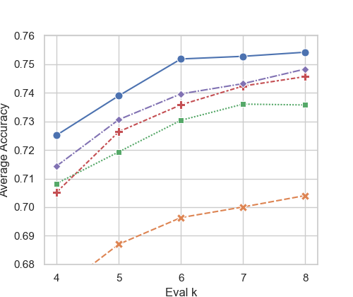
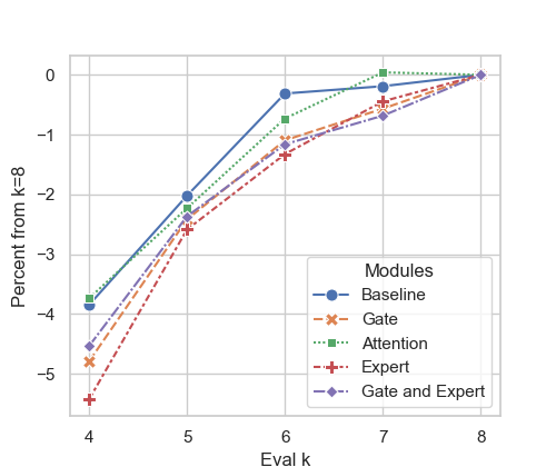
Figure 4: Average multiple choice QA accuracy vs. $k_{\mathrm{ev}}$ for parameter-subset refits for OLMoE-1B-7B-0125 on CommonSense170k with Oracle (left: average accuracy; right: relative accuracy reduction per parameter subset vs. $k_{\mathrm{ev}}=8$).

4 Related Work

Many-in-One Models.

Prior work enables a single network to run across compute budgets via global, pretraining-time sparsity or nested subnetworks. Slimmable and Once-for-All train width/subnet sets for CNNs (Yu et al., 2019; Yu & Huang, 2019; Li et al., 2021; Cai et al., 2020; Lou et al., 2021); transformer variants drop tokens or learn nested blocks (DynamicViT, ViT-Slimmable, Matryoshka, MatFormer) (Rao et al., 2021; Yin et al., 2022; Kusupati et al., 2022; Devvrit et al., 2024). For LLMs, Flextron fits routers post-training (Cai et al., 2024); pruning methods (e.g., retraining-free/Fisher) remove heads or filters (Kwon et al., 2022). These methods span multiple operating points but typically require bespoke pretraining, architecture changes, or storing multiple subnetworks.

Sparse MoEs.

Sparse MoEs are sparse models by design: a global sparsity parameter determines how many experts are active per token (Fedus et al., 2022; Riquelme et al., 2021). Subsequent work has explored richer forms of token-level sparsity. Token-aware schemes include probabilistic top-$k(P)$ gating (Huang et al., 2024), dynamic routing (Alizadeh-Vahid et al., 2024), the addition of null experts (Zeng et al., 2024; Team et al., 2025), and multiplier layers for experts in TC-Experts (Yan et al., 2025). Posttraining methods such as DynaMoE (Nishu et al., 2025) convert dense LLMs into token-sparse adaptive MoEs. Token-adaptive MoEs spend a fixed global budget more efficiently; PHDS changes the global budget at runtime. These approaches compose.

5 Discussion

In this paper, we (i) showed that pretrained sparse MoE models are more robust to runtime changes in sparsity than commonly assumed, (ii) demonstrated that sparsity can be an MoE serving primitive from a single checkpoint, and (iii) introduced MoE-PHDS, which allows practitioners to use SFT to make their existing models more robust to sparsity mis-specification. While naive SFT often works, MoE-PHDS provides added benefits for less tuned models and extends support across a slightly larger range of $k_{\mathrm{ev}}$. In practice, operators can often safely reduce $k$ by  20–30% with minimal loss, while larger reductions should be treated as best-effort. Although we evaluate moderate-scale MoEs, PHDS is most valuable where latency, energy, or memory are tight. Our experiments span models from 1B–14.3B parameters, a regime where memory and energy budgets are tightest. In these settings, multiple checkpoints are impractical and token-level adaptivity introduces variance, whereas a single global sparsity knob offers predictable accuracy–efficiency trade-offs without architectural changes. Higher cross-$k$ agreement further preserves the model’s “feel” as sparsity varies at runtime.

Limitations.

Results are from smaller models; scalability to larger ones is unknown. We study routed, equal-sized experts only; partial routing or heterogeneous expert sizes may behave differently. We also omit generation-heavy tasks (coding, summarization) and answer-style analyses, so some gains may reflect stylistic shifts rather than ability. Reported safe ranges are model and task dependent and need further study.

Reproducibility.

When possible, we used public models; we trained and evaluated on public data sets with standard harnesses. Diffs from OLMoE-1B-7B-0125 and Qwen1.5-MoE-A2.7B to support PHDS will be available in a git repo pending institutional approval, along with a .json file with experimental settings.

LLM Usage.

LLMs were used in this work for outlining, text editing, and literature search.

Appendix A Appendix

A.1 Literature Comparison

Positioning.

Literature is summarized in table 6. Prior work demonstrates that both dense and sparse models can be adapted to multiple computational settings, but with important limitations: dense models typically rely on pretraining across subnetworks or block structures, while MoEs fix a global sparsity parameter in advance. Token- or layer-level dynamic gating can be a powerful way to optimize how computational budget is spent for a fixed global sparsity level, but it injects variance (latency fluctuates with content) and adds policy complexity with additional tunable parameters. In contrast, to our knowledge, MoE-PHDS is the first method to enable global runtime sparsity control from a single checkpoint. Our approach only requires lightweight supervised fine tuning, avoids maintaining multiple subnetworks, and directly supports deployment across a set of operating points due to predictability, simplicity, and composability. Therefore this method complements, rather than competes with, finer-grained adaptivity.

Table 6: Comparison of methods enabling multiple operating points from a single model. MoE-PHDS uniquely supports global runtime sparsity control from a single checkpoint.

Method	Train	Runtime	Sparsity	Family
MoE (ours)
MoE-PHDS	SFT	Yes (1 checkpoint)	Global ($k$)	MoE
Dense Networks / FFNs
Slimmable (Yu et al., 2019)	Pre	Yes (width)	Global	CNN/FFN
US-Net (Yu & Huang, 2019)	Pre	Yes (width)	Global	CNN/FFN
OFA (Cai et al., 2020)	Pre	No	Global	FFN
Dyn-OFA (Cai et al., 2020)	Pre	Yes (stored nets)	Global	FFN
DS-Net (Lou et al., 2021)	Pre	Yes (stored filt.)	Global	FFN
MatFormer (Devvrit et al., 2024)	Pre	Yes (blocks)	Block	Trans.
Matryoshka (Kusupati et al., 2022)	Pre	Yes (nested)	Block	Trans.
Flextron (Cai et al., 2024)	Post	Yes (router)	Layer	LLM
RF-Pruning (Kwon et al., 2022)	Post	No	Head/Fil.	Trans.
Sparse MoEs
top-$k(P)$ (Huang et al., 2024)	Pre	No	Token	MoE
AdaMoE (Zeng et al., 2024)	Pre	No	Token	MoE
TC-MoE (Yan et al., 2025)	Pre	No	Token	MoE
DynaMoE (Nishu et al., 2025)	Post	No	Token	MoE/LLM
LongCat (Team et al., 2025)	Pre	No	Token	MoE

A.2 Experimental Settings

We used the settings summarized in table 7 for experiments. We run one seed for SFT (budget-constrained) and reuse that checkpoint across $k_{\mathrm{ev}}$; evaluation uses fixed harness seeds. For each we experiment, we ran a set of longer SFT trials to determine the number of tokens seen for mass ablations. Initial experiments were run for Oracle and PHDS settings, with a shortened schedule applied to all other ablations. Truncated schedule size was determined by where best checkpoints were selected in the initial run phases.

PHDS has three main tunble parameters: $\epsilon$, $\mathcal{K}_{\mathrm{train}}$, and Curriculum value. We chose $\epsilon$ by running ablations from 1E-1 to 1E-8; no material difference was seen below 1E-4, so we selected 1E-6 for all experiments. This value is large enough that there is some gradient flow and back propagation does not collapse, but small enough that changes when these values are included only have minor effects. The inclusion of a soft mask is also done for deployment ease, as methods like jax work best without changes to array sizes. In general, based on general performance across ablations, we use $\mathcal{K}_{\mathrm{train}}=\{k_{\mathrm{pre}}/2,\dots,k_{\mathrm{pre}}-1,k_{\mathrm{pre}}\}$.

Table 7: Experimental settings. LB is load balancing value.

Experiment	Initial Tokens	Ablation Tokens	GPUs	LB
Internal Baseline: CS170k	491M	246M	2xA100-40GB	0.01
Internal Baseline: Internal Data	393M	393M	8xA100-40GB	0.01
OLMoE: Tülu-3	39B	7.8B	8xA100-40GB	0.0
OLMoE: CS170k	327M	327M	8xA100-40GB	0.0
Qwen: Tülu-3	39B	7.8B	8xA100-40GB	0.0

A.3 Internal Baseline Models: CommonSense170K

Ablations on MoE-PHDS Parameters.

MoE-PHDS has two main tunable parameters: the sampling set, $\mathcal{K}_{\mathrm{train}}$, and the curriculum training values. In table 8, we train across sampling sets. In table 9, we fix a subset of sampling sets and train across curriculum values.

Table 8: Internal Baseline Models: CommonSense170k SFT, ablations across $\mathcal{K}_{\mathrm{train}}$ sets. Overall accuracy on CommonSense multiple choice. Best values are bold and second best underlined, grouped by $k_{\mathrm{pre}}$ and $k_{\mathrm{ev}}$. Untargeted $k_{\mathrm{ev}}$ are denoted by $--$.

Model	$k_{\mathrm{pre}}$	$k_{\mathrm{ev}}=2$	$k_{\mathrm{ev}}=3$	$k_{\mathrm{ev}}=4$	$k_{\mathrm{ev}}=5$	$k_{\mathrm{ev}}=6$
PHDS k=[2,3]	4	0.677000	0.708500	0.715625	–	–
PHDS k=[2,3] → 2	4	0.682875	0.713875	0.720500	–	–
PHDS k=[2,3,4]	4	0.678750	0.712000	0.718000	–	–
PHDS k=[2,3,4] → 2	4	0.695000	0.716500	0.717375	–	–
PHDS k=[2,4]	4	0.666625	0.698375	0.708750	–	–
PHDS k=[2,4] → 2	4	0.686625	0.716125	0.718875	–	–
PHDS k=[4,5]	6	–	0.683250	0.718875	0.729500	0.733250
PHDS k=[4,5] → 4	6	–	0.680750	0.720625	0.732000	0.740250
PHDS k=[4,5,6]	6	–	0.670250	0.706750	0.725000	0.730125
PHDS k=[4,5,6] → 4	6	–	0.692500	0.718250	0.731750	0.733625
PHDS k=[3,4,5,6]	6	–	0.694125	0.720250	0.728625	0.729375
PHDS k=[3,4,5,6] → 4	6	–	0.689875	0.723750	0.731375	0.734250

In experiments for table 8, we found that using all values between $k_{\mathrm{pre}}/2$ and $k_{\mathrm{pre}}$ produces consistently solid results. For higher $k_{\mathrm{pre}}$ values, non-inclusive subsets between $k_{\mathrm{pre}}/2$ and $k_{\mathrm{pre}}$ work well, and curriculum training consistently increases accuracy. In the experiments for table 9, we found that the best results are consistently from $k$ just above $k_{\mathrm{pre}}/2$, and that results are consistent across $\mathcal{K}_{\mathrm{train}}$ groups based given $k_{\mathrm{pre}}$.

Table 9: CommonSense 170k Fine-tuning: overall accuracy by $\mathcal{K}_{\mathrm{train}}$ and curriculum.

v Model	$k_{\mathrm{pre}}$	$k_{\mathrm{ev}}=2$	$k_{\mathrm{ev}}=3$	$k_{\mathrm{ev}}=4$	$k_{\mathrm{ev}}=5$	$k_{\mathrm{ev}}=6$
PHDS k=[2,3,4]	4	0.678750	0.712000	0.718000	–	–
PHDS k=[2,3,4] → 1	4	0.675125	0.700375	0.708375	–	–
PHDS k=[2,3,4] → 2	4	0.695000	0.716500	0.717375	–	–
PHDS k=[2,3,4] → 3	4	0.708500	0.714000	0.723875	–	–
PHDS k=[2,3,4] → 4	4	0.666250	0.706750	0.714625	–	–
PHDS k=[4,5]	6	–	0.683250	0.718875	0.729500	0.733250
PHDS k=[4,5] → 2	6	–	0.679500	0.713750	0.717875	0.723125
PHDS k=[4,5] → 3	6	–	0.668750	0.704250	0.713875	0.715625
PHDS k=[4,5] → 4	6	–	0.680750	0.720625	0.732000	0.740250
PHDS k=[4,5] → 5	6	–	0.676875	0.716250	0.728875	0.733375
PHDS k=[4,5] → 6	6	–	0.574500	0.622750	0.729000	0.733250
PHDS k=[3,4,5,6]	6	–	0.694125	0.720250	0.728625	0.729375
PHDS k=[3,4,5,6] → 2	6	–	0.677500	0.706750	0.718375	0.721125
PHDS k=[3,4,5,6] → 3	6	–	0.695125	0.704250	0.724625	0.722500
PHDS k=[3,4,5,6] → 4	6	–	0.689875	0.723750	0.731375	0.734250
PHDS k=[3,4,5,6] → 5	6	–	0.680750	0.711875	0.723000	0.725125
PHDS k=[3,4,5,6] → 6	6	–	0.574500	0.719875	0.728875	0.732875

A.4 OLMoE Experiments

Full results from OLMoE on Tülu-3 is given in tables 10 and 11.

Table 10: OLMoE fine-tuned on Tülu-3. Best per block in bold, second-best underlined. Well-specified methods are in blue.

OLMoE-1B-7B-0125-Instruct
Model	ARC-C	ARC-E	boolq	hella	piqa	sciq	wino	Avg	triv	wiki
$k_{\mathrm{ev}}=8$
Oracle	0.4642	0.7412	0.7563	0.5977	0.7622	0.949	0.6764	0.7067	0.3977	15.810
[4,…,8]→5	0.4701	0.7336	0.7615	0.5950	0.7590	0.956	0.6725	0.7068	0.4131	15.742
[4,5,6,7,8]	0.4642	0.7340	0.7596	0.5932	0.7644	0.948	0.6654	0.7041	0.4119	15.484
8→4	0.4701	0.7370	0.7599	0.5941	0.7617	0.949	0.6693	0.7059	0.4174	15.488
$k_{\mathrm{ev}}=7$
Oracle	0.4582	0.7391	0.7563	0.5922	0.7601	0.950	0.6598	0.7022	0.3902	16.238
[4,…,8]→5	0.4582	0.7294	0.7563	0.5945	0.7606	0.948	0.6575	0.7006	0.3928	16.280
[4,5,6,7,8]	0.4608	0.7231	0.7575	0.5928	0.7552	0.951	0.6590	0.6999	0.3973	16.014
8→4	0.4633	0.7298	0.7575	0.5909	0.7617	0.949	0.6535	0.7008	0.4003	16.042
$k_{\mathrm{ev}}=6$
Oracle	0.4471	0.7201	0.7609	0.5895	0.7590	0.947	0.6433	0.6953	0.3756	17.372
[4,…,8]→5	0.4437	0.7142	0.7667	0.5884	0.7514	0.951	0.6385	0.6934	0.3842	17.426
[4,5,6,7,8]	0.4352	0.7130	0.7590	0.5878	0.7503	0.951	0.6377	0.6906	0.3862	17.148
8→4	0.4428	0.7205	0.7606	0.5871	0.7563	0.947	0.6464	0.6943	0.3909	17.188
$k_{\mathrm{ev}}=5$
Oracle	0.4334	0.7029	0.7413	0.5774	0.7443	0.947	0.6393	0.6837	0.3686	19.687
[4,…,8]→5	0.4300	0.7054	0.7468	0.5742	0.7437	0.943	0.6385	0.6831	0.3745	19.775
[4,5,6,7,8]	0.4232	0.6944	0.7419	0.5743	0.7508	0.946	0.6243	0.6793	0.3695	19.534
8→4	0.4377	0.7050	0.7419	0.5721	0.7481	0.948	0.6401	0.6847	0.3700	19.621
$k_{\mathrm{ev}}=4$
Oracle	0.3805	0.6894	0.7287	0.5543	0.7296	0.942	0.6140	0.6627	0.3304	24.574
[4,…,8]→5	0.3899	0.6814	0.7278	0.5509	0.7394	0.939	0.6267	0.6650	0.3339	24.921
[4,5,6,7,8]	0.3823	0.6692	0.7242	0.5472	0.7329	0.937	0.6133	0.6580	0.3305	24.640
8→4	0.3874	0.6768	0.7196	0.5490	0.7301	0.938	0.6212	0.6603	0.3316	24.965

Table 11: OLMoE fine-tuned on Tülu-3. Best per block in bold, second-best underlined. Well-specified methods are in blue.

OLMoE-1B-7B-0125
Model	ARC-C	ARC-E	boolq	hella	piqa	sciq	wino	Avg	triv	wiki
$k_{\mathrm{ev}}=8$
Oracle	0.4582	0.7757	0.7040	0.5673	0.7797	0.955	0.6953	0.7050	0.4889	9.407
[4,…,8]→5	0.4471	0.7605	0.6997	0.5742	0.7856	0.932	0.6985	0.6997	0.4585	8.923
[4,5,6,7,8]	0.4659	0.7694	0.7070	0.5764	0.7856	0.937	0.6946	0.7051	0.4901	8.903
8→4	0.4573	0.7668	0.7043	0.5635	0.7862	0.943	0.6938	0.7021	0.4794	9.485
$k_{\mathrm{ev}}=7$
Oracle	0.4497	0.7723	0.7018	0.5680	0.7835	0.951	0.6859	0.7017	0.4928	9.557
[4,…,8]→5	0.4428	0.7508	0.6899	0.5747	0.7835	0.932	0.6835	0.6939	0.4578	9.075
[4,5,6,7,8]	0.4531	0.7626	0.7061	0.5757	0.7835	0.934	0.6859	0.7001	0.4815	9.056
8→4	0.4565	0.7597	0.6896	0.5666	0.7786	0.944	0.6811	0.6966	0.4793	9.639
$k_{\mathrm{ev}}=6$
Oracle	0.4403	0.7677	0.7009	0.5665	0.7780	0.952	0.6717	0.6967	0.4817	9.985
[4,…,8]→5	0.4471	0.7479	0.6865	0.5703	0.7780	0.928	0.6669	0.6893	0.4667	9.496
[4,5,6,7,8]	0.4565	0.7534	0.6994	0.5726	0.7840	0.934	0.6764	0.6966	0.4767	9.474
8→4	0.4445	0.7500	0.6884	0.5637	0.7856	0.938	0.6764	0.6924	0.4737	10.091
$k_{\mathrm{ev}}=5$
Oracle	0.4206	0.7370	0.6957	0.5559	0.7704	0.942	0.6725	0.6849	0.4487	10.975
[4,…,8]→5	0.4078	0.7151	0.6841	0.5619	0.7629	0.934	0.6535	0.6742	0.4242	10.431
[4,5,6,7,8]	0.4206	0.7311	0.7028	0.5630	0.7720	0.933	0.6527	0.6822	0.4293	10.408
8→4	0.4232	0.7323	0.6865	0.5540	0.7709	0.934	0.6630	0.6806	0.4448	11.151
$k_{\mathrm{ev}}=4$
Oracle	0.4053	0.7109	0.6706	0.5386	0.7628	0.930	0.6338	0.6646	0.3787	13.032
[4,…,8]→5	0.3984	0.6949	0.6722	0.5443	0.7584	0.920	0.6251	0.6590	0.3605	12.357
[4,5,6,7,8]	0.4138	0.7024	0.6798	0.5471	0.7661	0.927	0.6314	0.6668	0.3775	12.304
8→4	0.3993	0.7020	0.6648	0.5369	0.7633	0.909	0.6354	0.6587	0.3886	13.424

A.5 Qwen

Full results for Qwen on Tülu-3 are given in table 12.

Table 12: Qwen: fine-tuned on Tülu-3 for the untuned model. Best per block in bold, second-best underlined. Well-specified methods are in blue.

Qwen1.5-MoE-A2.7B
Model	ARC-C	ARC-E	boolq	hella	piqa	sciq	wino	Avg	triv	wiki
$k_{\mathrm{ev}}=4$
Oracle	0.4104	0.7302	0.7911	0.5806	0.7982	0.945	0.6906	0.7069	0.0287	10.223
[2,3,4]→2	0.4172	0.7273	0.7884	0.5798	0.8020	0.942	0.6946	0.7073	0.0271	10.244
[2,3,4]	0.4121	0.7290	0.7859	0.5805	0.7987	0.942	0.6930	0.7059	0.0269	10.227
4→2	0.4172	0.7298	0.7920	0.5813	0.7987	0.944	0.6875	0.7072	0.0284	10.225
$k_{\mathrm{ev}}=3$
Oracle	0.4002	0.7281	0.7872	0.5781	0.7976	0.949	0.6946	0.7050	0.0337	10.355
[2,3,4]→2	0.4044	0.7252	0.7887	0.5759	0.7965	0.948	0.6914	0.7043	0.0329	10.367
[2,3,4]	0.3985	0.7302	0.7905	0.5766	0.7976	0.947	0.6851	0.7036	0.0317	10.364
4→2	0.4019	0.7319	0.7893	0.5775	0.7992	0.949	0.6938	0.7061	0.0342	10.353
$k_{\mathrm{ev}}=2$
Oracle	0.4027	0.7146	0.7789	0.5680	0.7938	0.946	0.6622	0.6952	0.0334	10.810
[2,3,4]→2	0.4019	0.7092	0.7746	0.5658	0.7884	0.946	0.6646	0.6929	0.0342	10.832
[2,3,4]	0.3959	0.7075	0.7774	0.5673	0.7884	0.946	0.6669	0.6928	0.0317	10.821
4→2	0.4002	0.7113	0.7786	0.5680	0.7938	0.946	0.6535	0.6931	0.0341	10.811
Qwen1.5-MoE-A2.7B-Chat
Model	ARC-C	ARC-E	boolq	hella	piqa	sciq	wino	Avg	triv	wiki
$k_{\mathrm{ev}}=4$
Oracle	0.3985	0.7012	0.8089	0.5936	0.7894	0.947	0.6622	0.7001	0.0563	11.436
[2,3,4]→2	0.4002	0.7029	0.8080	0.5950	0.7861	0.946	0.6653	0.7005	0.0585	11.373
[2,3,4]	0.3985	0.7029	0.8061	0.5943	0.7927	0.949	0.6717	0.7022	0.0631	11.331
4→2	0.3951	0.7045	0.8076	0.5936	0.7900	0.948	0.6661	0.7007	0.0526	11.420
$k_{\mathrm{ev}}=3$
Oracle	0.3951	0.7003	0.8037	0.5914	0.7840	0.949	0.6567	0.6972	0.0633	11.608
[2,3,4]→2	0.3959	0.7033	0.8082	0.5928	0.7845	0.947	0.6535	0.6979	0.0642	11.549
[2,3,4]	0.3908	0.7029	0.8046	0.5921	0.7845	0.949	0.6535	0.6968	0.0664	11.502
4→2	0.4027	0.7037	0.8058	0.5908	0.7872	0.943	0.6614	0.6992	0.0661	11.605
$k_{\mathrm{ev}}=2$
Oracle	0.3831	0.6848	0.7758	0.5802	0.7726	0.945	0.6330	0.6821	0.0625	12.225
[2,3,4]→2	0.3865	0.6827	0.7728	0.5821	0.7726	0.944	0.6511	0.6845	0.0662	12.070
[2,3,4]	0.3968	0.6835	0.7729	0.5813	0.7780	0.943	0.6425	0.6854	0.0675	12.033
4→2	0.3959	0.6789	0.7716	0.5797	0.7742	0.946	0.6385	0.6835	0.0643	12.132

A.6 Mechanisms of Robustness at Reduced $k$

Setup.

On OLMoE-1B-7B-0125, we SFT on CommonSense170K with subset refits: Baseline, Gate, Expert, Attention, Expert and Gate, under Oracle and PHDS [4,5,6,7,8]→5 regimes. Curriculum scheduling is introduced to PHDS after 93.9% of epoch 1; all runs are done through two full epochs. Checkpoints are selected by best MC-QA accuracy at $k_{\mathrm{ev}}{=}8$.

Metrics.

Overall MC-QA accuracy and relative drop vs. accuracy for $k_{\mathrm{ev}}=8$ by parameter subset. Metrics are reported by parameter subset to understand which subsets have less relative degradation at low $k_{\mathrm{ev}}$, even if they have poorer fits at $k_{\mathrm{ev}}=8$.

Findings.

Our results with MoE-PHDS are similar to those for Oracle, with Expert adding the majority of fit value at $k_{\mathrm{ev}}=8$, but with Attention contributing significant value at $k_{\mathrm{ev}}=4$.

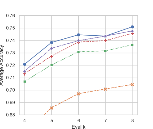
Figure 5: Average multiple choice QA accuracy vs. $k_{\mathrm{ev}}$ for parameter-subset refits for OLMoE-1B-7B-0125 on CommonSense170k with PHDS [4,5,6,7,8]→5 (left: average accuracy; right: relative drop per parameter subset vs. $k_{\mathrm{ev}}=8$).

References

- Alizadeh-Vahid et al. (2024) Keivan Alizadeh-Vahid, Seyed Iman Mirzadeh, Hooman Shahrkokhi, Dmitry Belenko, Frank Sun, Minsik Cho, Mohammad Hossein Sekhavat, Moin Nabi, and Mehrdad Farajtabar. Duo-llm: A framework for studying adaptive computation in large language models. In NeurIPS Efficient Natural Language and Speech Processing Workshop, pp. 443–455. PMLR, 2024.
- Bisk et al. (2020) Yonatan Bisk, Rowan Zellers, Jianfeng Gao, Yejin Choi, et al. Piqa: Reasoning about physical commonsense in natural language. In Proceedings of the AAAI conference on artificial intelligence, volume 34, pp. 7432–7439, 2020.
- Cai et al. (2020) Han Cai, Chuang Gan, Tianzhe Wang, Zhekai Zhang, and Song Han. Once for all: Train one network and specialize it for efficient deployment. In International Conference on Learning Representations, 2020.
- Cai et al. (2024) Ruisi Cai, Saurav Muralidharan, Greg Heinrich, Hongxu Yin, Zhangyang Wang, Jan Kautz, and Pavlo Molchanov. Flextron: Many-in-one flexible large language model. In International Conference on Machine Learning, pp. 5298–5311. PMLR, 2024.
- Clark et al. (2019) Christopher Clark, Kenton Lee, Ming-Wei Chang, Tom Kwiatkowski, Michael Collins, and Kristina Toutanova. Boolq: Exploring the surprising difficulty of natural yes/no questions. arXiv preprint arXiv:1905.10044, 2019.
- Clark et al. (2018) Peter Clark, Isaac Cowhey, Oren Etzioni, Tushar Khot, Ashish Sabharwal, Carissa Schoenick, and Oyvind Tafjord. Think you have solved question answering? Try ARC, the AI2 reasoning challenge. arXiv preprint arXiv:1803.05457, 2018.
- Devvrit et al. (2024) Fnu Devvrit, Sneha Kudugunta, Aditya Kusupati, Tim Dettmers, Kaifeng Chen, Inderjit Dhillon, Yulia Tsvetkov, Hanna Hajishirzi, Sham Kakade, Ali Farhadi, et al. Matformer: Nested transformer for elastic inference. Advances in Neural Information Processing Systems, 37:140535–140564, 2024.
- Du et al. (2022) Nan Du, Yanping Huang, Andrew M Dai, Simon Tong, Dmitry Lepikhin, Yuanzhong Xu, Maxim Krikun, Yanqi Zhou, Adams Wei Yu, Orhan Firat, Barret Zoph, Liam Fedus, Maarten P Bosma, Zongwei Zhou, Tao Wang, Emma Wang, Kellie Webster, Marie Pellat, Kevin Robinson, Kathleen Meier-Hellstern, Toju Duke, Lucas Dixon, Kun Zhang, Quoc Le, Yonghui Wu, Zhifeng Chen, and Claire Cui. GLaM: Efficient scaling of language models with mixture-of-experts. In Kamalika Chaudhuri, Stefanie Jegelka, Le Song, Csaba Szepesvari, Gang Niu, and Sivan Sabato (eds.), Proceedings of the 39th International Conference on Machine Learning, volume 162 of Proceedings of Machine Learning Research, pp. 5547–5569. PMLR, 17–23 Jul 2022. URL https://proceedings.mlr.press/v162/du22c.html.
- Fedus et al. (2022) William Fedus, Barret Zoph, and Noam Shazeer. Switch transformers: Scaling to trillion parameter models with simple and efficient sparsity. Journal of Machine Learning Research, 23(120):1–39, 2022.
- Hu et al. (2023) Zhiqiang Hu, Yihuai Lan, Lei Wang, Wanyu Xu, Ee-Peng Lim, Roy Ka-Wei Lee, Lidong Bing, and Soujanya Poria. Llm-adapters: An adapter family for parameter-efficient fine-tuning of large language models. arXiv preprint arXiv:2304.01933, 2023.
- Huang et al. (2024) Quzhe Huang, Zhenwei An, Nan Zhuang, Mingxu Tao, Chen Zhang, Yang Jin, Kun Xu, Liwei Chen, Songfang Huang, and Yansong Feng. Harder task needs more experts: Dynamic routing in moe models. In Proceedings of the 62nd Annual Meeting of the Association for Computational Linguistics (Volume 1: Long Papers), pp. 12883–12895, 2024.
- Joshi et al. (2017) Mandar Joshi, Eunsol Choi, Daniel S Weld, and Luke Zettlemoyer. Triviaqa: A large scale distantly supervised challenge dataset for reading comprehension. arXiv preprint arXiv:1705.03551, 2017.
- Kusupati et al. (2022) Aditya Kusupati, Gantavya Bhatt, Aniket Rege, Matthew Wallingford, Aditya Sinha, Vivek Ramanujan, William Howard-Snyder, Kaifeng Chen, Sham Kakade, Prateek Jain, et al. Matryoshka representation learning. Advances in Neural Information Processing Systems, 35:30233–30249, 2022.
- Kwon et al. (2022) Woosuk Kwon, Sehoon Kim, Michael W Mahoney, Joseph Hassoun, Kurt Keutzer, and Amir Gholami. A fast post-training pruning framework for transformers. Advances in Neural Information Processing Systems, 35:24101–24116, 2022.
- Lambert et al. (2024) Nathan Lambert, Jacob Morrison, Valentina Pyatkin, Shengyi Huang, Hamish Ivison, Faeze Brahman, Lester James V. Miranda, Alisa Liu, Nouha Dziri, Shane Lyu, Yuling Gu, Saumya Malik, Victoria Graf, Jena D. Hwang, Jiangjiang Yang, Ronan Le Bras, Oyvind Tafjord, Chris Wilhelm, Luca Soldaini, Noah A. Smith, Yizhong Wang, Pradeep Dasigi, and Hannaneh Hajishirzi. Tülu 3: Pushing frontiers in open language model post-training. 2024.
- Li et al. (2021) Changlin Li, Guangrun Wang, Bing Wang, Xiaodan Liang, Zhihui Li, and Xiaojun Chang. Dynamic slimmable network. In Proceedings of the IEEE/CVF Conference on Computer Vision and Pattern Recognition (CVPR), pp. 8607–8617, June 2021.
- Liu et al. (2024) Aixin Liu, Bei Feng, Bing Xue, Bingxuan Wang, Bochao Wu, Chengda Lu, Chenggang Zhao, Chengqi Deng, Chenyu Zhang, Chong Ruan, et al. Deepseek-v3 technical report. arXiv preprint arXiv:2412.19437, 2024.
- Lou et al. (2021) Wei Lou, Lei Xun, Amin Sabet, Jia Bi, Jonathon Hare, and Geoff V Merrett. Dynamic-ofa: Runtime dnn architecture switching for performance scaling on heterogeneous embedded platforms. In Proceedings of the IEEE/CVF Conference on Computer Vision and Pattern Recognition, pp. 3110–3118, 2021.
- Merity et al. (2016) Stephen Merity, Caiming Xiong, James Bradbury, and Richard Socher. Pointer sentinel mixture models. arXiv preprint arXiv:1609.07843, 2016.
- Mihaylov et al. (2018) Todor Mihaylov, Peter Clark, Tushar Khot, and Ashish Sabharwal. Can a suit of armor conduct electricity? a new dataset for open book question answering. arXiv preprint arXiv:1809.02789, 2018.
- Muennighoff et al. (2024) Niklas Muennighoff, Luca Soldaini, Dirk Groeneveld, Kyle Lo, Jacob Morrison, Sewon Min, Weijia Shi, Pete Walsh, Oyvind Tafjord, Nathan Lambert, Yuling Gu, Shane Arora, Akshita Bhagia, Dustin Schwenk, David Wadden, Alexander Wettig, Binyuan Hui, Tim Dettmers, Douwe Kiela, Ali Farhadi, Noah A. Smith, Pang Wei Koh, Amanpreet Singh, and Hannaneh Hajishirzi. Olmoe: Open mixture-of-experts language models, 2024. URL https://arxiv.org/abs/2409.02060.
- Nishu et al. (2025) Kumari Nishu, Sachin Mehta, Samira Abnar, Mehrdad Farajtabar, Maxwell Horton, Mahyar Najibi, Moin Nabi, Minsik Cho, and Devang Naik. From dense to dynamic: Token-difficulty driven moefication of pre-trained llms. arXiv preprint arXiv:2502.12325, 2025.
- Qwen Team (2024) Qwen Team. Qwen1.5-moe: Matching 7b model performance with 1/3 activated parameters”, February 2024. URL https://qwenlm.github.io/blog/qwen-moe/.
- Rao et al. (2021) Yongming Rao, Wenliang Zhao, Benlin Liu, Jiwen Lu, Jie Zhou, and Cho-Jui Hsieh. Dynamicvit: Efficient vision transformers with dynamic token sparsification. Advances in neural information processing systems, 34:13937–13949, 2021.
- Riquelme et al. (2021) Carlos Riquelme, Joan Puigcerver, Basil Mustafa, Maxim Neumann, Rodolphe Jenatton, André Susano Pinto, Daniel Keysers, and Neil Houlsby. Scaling vision with sparse mixture of experts. Advances in Neural Information Processing Systems, 34:8583–8595, 2021.
- Sakaguchi et al. (2021) Keisuke Sakaguchi, Ronan Le Bras, Chandra Bhagavatula, and Yejin Choi. Winogrande: An adversarial winograd schema challenge at scale. Communications of the ACM, 64(9):99–106, 2021.
- Sap et al. (2019) Maarten Sap, Hannah Rashkin, Derek Chen, Ronan LeBras, and Yejin Choi. Socialiqa: Commonsense reasoning about social interactions. arXiv preprint arXiv:1904.09728, 2019.
- Team et al. (2025) Meituan LongCat Team, Bayan, Bei Li, Bingye Lei, Bo Wang, Bolin Rong, Chao Wang, Chao Zhang, Chen Gao, Chen Zhang, Cheng Sun, Chengcheng Han, Chenguang Xi, Chi Zhang, Chong Peng, Chuan Qin, Chuyu Zhang, Cong Chen, Congkui Wang, Dan Ma, Daoru Pan, Defei Bu, Dengchang Zhao, Deyang Kong, Dishan Liu, Feiye Huo, Fengcun Li, Fubao Zhang, Gan Dong, Gang Liu, Gang Xu, Ge Li, Guoqiang Tan, Guoyuan Lin, Haihang Jing, Haomin Fu, Haonan Yan, Haoxing Wen, Haozhe Zhao, Hong Liu, Hongmei Shi, Hongyan Hao, Hongyin Tang, Huantian Lv, Hui Su, Jiacheng Li, Jiahao Liu, Jiahuan Li, Jiajun Yang, Jiaming Wang, Jian Yang, Jianchao Tan, Jiaqi Sun, Jiaqi Zhang, Jiawei Fu, Jiawei Yang, Jiaxi Hu, Jiayu Qin, Jingang Wang, Jiyuan He, Jun Kuang, Junhui Mei, Kai Liang, Ke He, Kefeng Zhang, Keheng Wang, Keqing He, Liang Gao, Liang Shi, Lianhui Ma, Lin Qiu, Lingbin Kong, Lingtong Si, Linkun Lyu, Linsen Guo, Liqi Yang, Lizhi Yan, Mai Xia, Man Gao, Manyuan Zhang, Meng Zhou, Mengxia Shen, Mingxiang Tuo, Mingyang Zhu, Peiguang Li, Peng Pei, Peng Zhao, Pengcheng Jia, Pingwei Sun, Qi Gu, Qianyun Li, Qingyuan Li, Qiong Huang, Qiyuan Duan, Ran Meng, Rongxiang Weng, Ruichen Shao, Rumei Li, Shizhe Wu, Shuai Liang, Shuo Wang, Suogui Dang, Tao Fang, Tao Li, Tefeng Chen, Tianhao Bai, Tianhao Zhou, Tingwen Xie, Wei He, Wei Huang, Wei Liu, Wei Shi, Wei Wang, Wei Wu, Weikang Zhao, Wen Zan, Wenjie Shi, Xi Nan, Xi Su, Xiang Li, Xiang Mei, Xiangyang Ji, Xiangyu Xi, Xiangzhou Huang, Xianpeng Li, Xiao Fu, Xiao Liu, Xiao Wei, Xiaodong Cai, Xiaolong Chen, Xiaoqing Liu, Xiaotong Li, Xiaowei Shi, Xiaoyu Li, Xili Wang, Xin Chen, Xing Hu, Xingyu Miao, Xinyan He, Xuemiao Zhang, Xueyuan Hao, Xuezhi Cao, Xunliang Cai, Xurui Yang, Yan Feng, Yang Bai, Yang Chen, Yang Yang, Yaqi Huo, Yerui Sun, Yifan Lu, Yifan Zhang, Yipeng Zang, Yitao Zhai, Yiyang Li, Yongjing Yin, Yongkang Lv, Yongwei Zhou, Yu Yang, Yuchen Xie, Yueqing Sun, Yuewen Zheng, Yuhua Wei, Yulei Qian, Yunfan Liang, Yunfang Tai, Yunke Zhao, Zeyang Yu, Zhao Zhang, Zhaohua Yang, Zhenchao Zhang, Zhikang Xia, Zhiye Zou, Zhizhao Zeng, Zhongda Su, Zhuofan Chen, Zijian Zhang, Ziwen Wang, Zixu Jiang, Zizhe Zhao, Zongyu Wang, and Zunhai Su. Longcat-flash technical report, 2025. URL https://arxiv.org/abs/2509.01322.
- Welbl et al. (2017) Johannes Welbl, Nelson F Liu, and Matt Gardner. Crowdsourcing multiple choice science questions. arXiv preprint arXiv:1707.06209, 2017.
- Yan et al. (2025) Shen Yan, Xingyan Bin, Sijun Zhang, Yisen Wang, and Zhouchen Lin. TC-MoE: Augmenting Mixture of Experts with Ternary Expert Choice. In The Thirteenth International Conference on Learning Representations, 2025.
- Yin et al. (2022) Hongxu Yin, Arash Vahdat, Jose M Alvarez, Arun Mallya, Jan Kautz, and Pavlo Molchanov. A-vit: Adaptive tokens for efficient vision transformer. In Proceedings of the IEEE/CVF conference on computer vision and pattern recognition, pp. 10809–10818, 2022.
- Yu & Huang (2019) Jiahui Yu and Thomas S. Huang. Universally slimmable networks and improved training techniques. In Proceedings of the IEEE/CVF International Conference on Computer Vision (ICCV), October 2019.
- Yu et al. (2019) Jiahui Yu, Linjie Yang, Ning Xu, Jianchao Yang, and Thomas Huang. Slimmable neural networks. In 7th International Conference on Learning Representations, ICLR 2019, 2019.
- Zellers et al. (2019) Rowan Zellers, Ari Holtzman, Yonatan Bisk, Ali Farhadi, and Yejin Choi. Hellaswag: Can a machine really finish your sentence? arXiv preprint arXiv:1905.07830, 2019.
- Zeng et al. (2024) Zihao Zeng, Yibo Miao, Hongcheng Gao, Hao Zhang, and Zhijie Deng. Adamoe: Token-adaptive routing with null experts for mixture-of-experts language models. In Findings of the Association for Computational Linguistics: EMNLP 2024, pp. 6223–6235, 2024.