Numerical solution of the unsteady Brinkman equations in the framework of $H$(div)-conforming finite element methods

Abstract

We present projection-based mixed finite element methods for the solution of the unsteady Brinkman equations for incompressible single-phase flow with fixed in space porous solid inclusions. At each time step the method requires the solution of a predictor and a projection problem. The predictor problem, which uses a stress-velocity mixed formulation, accounts for the momentum balance, while the projection problem, which is based on a velocity-pressure mixed formulation, accounts for the incompressibility. The spatial discretization is $H$(div)-conforming and the velocity computed at the end of each time step is pointwise divergence-free. Unconditional stability of the fully-discrete scheme and first order in time accuracy are established. Due to the $H$(div)-conformity of the formulation, the methods are robust in both the Stokes and the Darcy regimes. In the specific code implementation, we discretize the computational domain using the Raviart–Thomas space $RT_{1}$ in two and three dimensions, applying a second-order accurate multipoint flux mixed finite element scheme with a quadrature rule that samples the flux degrees of freedom. In the predictor problem this allows for a local elimination of the viscous stress and results in element-based symmetric and positive definite systems for each velocity component with $\left(d+1\right)$ degrees of freedom per simplex (where $d$ is the dimension of the problem). In a similar way, we locally eliminate the corrected velocity in the projection problem and solve an element-based system for the pressure. Numerical experiments are presented to verify the convergence of the proposed scheme and illustrate its performance for several challenging applications, including one-domain modeling of coupled free fluid and porous media flows and heterogeneous porous media with strong discontinuity of the porosity and permeability values.

[label1]organization=Department of Engineering, University of Palermo, addressline=viale delle Scienze, city=Palermo, postcode=90128, country=Italy

[label2]organization=Institute for Modelling Hydraulic and Environmental Systems (IWS), Department of Hydromechanics and Modelling of Hydrosystems, University of Stuttgart, addressline=Pfaffenwaldring 61, city=Stuttgart, postcode=D-70569, country=Germany

[label3]organization=Department of Mathematics, University of Pittsburgh, addressline=301 Thackeray Hall, city=Pittsburgh, postcode=PA 15260, country=USA

1 Introduction

The Brinkman equations brinkman1949calculation can be considered as a combination of the Stokes and Darcy models, with a viscous term added to Darcy’s law. The model has important industrial, biomedical, and environmental applications, when the porous medium has heterogeneous porosity/permeability values, in such a way that in some portions of the domain the flow is governed by Darcy’s law and elsewhere by the Stokes equations, e.g., flow around or within foams, fuel cells, heat exchangers, drying and filtration processes, flows in biological tissues, and groundwater flow in fractured porous media. The Brinkman equations are derived from the volume averaging of the pore-scale Stokes equations at the continuum representative elementary volume (REV) scale CHANDESRIS20062137 , LeBarsWorster2006 . Pore-scale simulations are accurate, but computationally expensive due to the high number of grid elements needed to discretize the void spaces in the porous medium. Additionally, a detailed knowledge of the solid inclusion geometry is often missing. For these reasons continuum REV scale approaches have become popular. The Brinkman model includes porosity and permeability parameters, which can vary spatially. Thus, the model allows for flow in either the Stokes or the Darcy regimes in different regions, using the so called “one-domain approach” (ODA) with a single “fictitious” medium and one set of governing equations. The Brinkman equations represent an alternative way to model the coupling of Stokes and Darcy equations through interface conditions LSY , Riv-Yot , Vas-Yot , Lipnikov2014 , KANSCHAT20105933 , CAMANO2015362 , Boon2024 , gos2011 .

One of the most challenging aspects of the numerical approximation of the Brinkman equations is the construction of stable and robust methods in both the Stokes and the Darcy regimes. Standard inf-sup stable velocity-pressure mixed finite element (MFE) methods for the Stokes equations, such as the MINI and the Taylor–Hood elements, provide suboptimal convergence orders in the Darcy regime MarTaiWin . On the other hand, stable $H$(div)-conforming mixed Darcy elements, like the Raviart–Thomas or the Brezzi–Douglas–Marini elements, do not satisfy the required $H^{1}$-conformity in the Stokes regime. Various approaches have been developed, including enhancing stable Darcy elements to enforce some tangential continuity MarTaiWin , GuzmNeil-Brinkman , XieXuXue , penalized $H$(div)-conforming methods Konno-Stenberg , Konno2012-lt , KANSCHAT20105933 , stabilized methods based on Stokes elements Burman-Brinkman , Burman-SD , Badia-Codina , Nafa , Masud , JunSten-Brinkman , CORREA20092710 , Arbogast-SD , and weak Galerkin methods Mu-Hdiv-WG , Mu-Wang-Ye .

The above mentioned methods are based on the standard velocity-pressure formulation, where the velocity is approximated in the (possibly broken) $H^{1}$-norm, which makes it difficult to obtain robustness in both the Stokes and the Darcy regimes. An alternative approach is to consider dual mixed formulations, where the stress or the pseudostress is introduced as a primary variable and the velocity is approximated in the $L^{2}$-norm Qian , Gatica-pseudostress-Brinkman , BustGatGonz , Howel-dual-mixed-Brinkman , Zhao-Brinkman , Caucao-Yotov , BF-three-field . In these schemes, the mass conservation is only weakly imposed and the approximation of the velocity is discontinuous. Vorticity-based mixed formulations with $H$(div)-conforming velocity are developed in Vassilevski , Anaya , while an augmented vorticity-based mixed method with $H^{1}$-conforming velocity is proposed in BF-vorticity .

In this paper we develop a family of new $H$(div)-conforming projection-based MFE methods for the unsteady Brinkman equations, which provide pointwise divergence-free velocity. Moreover, due to the $H$(div)-conformity of the formulation, the methods are robust in both the Stokes and the Darcy regimes. Extending the methodology proposed in ARICO2025117616 for the unsteady Stokes equations (see also Arico-NS-RT0 , Arico-ODA ), we apply an incremental pressure correction method in the framework of projection schemes BROWN2001464 , GUERMOND2006 . At each time step we solve a predictor problem for the viscous term, followed by a projection problem to incorporate the incompressibility constraint. The predictor problem uses a mixed stress-velocity formulation Cai-MFE-NS , gos2011 , whereas the projection problem is based on a mixed velocity-pressure formulation. The stable MFE spaces Brezzi–Douglas–Marini ($BDM_{k}$), $k\geq 1$, or Raviart–Thomas ($RT_{k}$), $k\geq 0$, on simplicial grids BBF are considered for the components of the viscous stress in the predictor problem and the velocity in the projection problem. The velocity at the end of each time iteration is $H$(div)-conforming and divergence-free polynomial of degree $\leq k$. We establish unconditional stability of the fully discrete method, obtaining bounds on the viscous stress and the velocity that are robust in both the Stokes and Darcy limits. We then derive a first-order in time error bound for the semi-discrete continuous-in-space scheme.

A specific second-order in space method based on the $RT_{1}$ space and discontinuous piecewise linear polynomials on unstructured triangular or tetrahedral grids is developed in the second part of the paper. We avoid the solution of saddle point problems by employing the multipoint flux mixed finite element (MFMFE) method, which was originally proposed for Darcy flow as a first-order method in W-Y using the $BDM_{1}$ space and extended to a second-order method based on the $RT_{1}$ space in Radu , see also Caucao2020AMS for the multipoint stress mixed finite element for the Stokes equations. A quadrature rule that samples the flux degrees of freedom allows for mass lumping and local elimination of the stress in the predictor problem and the velocity in the projection problem. As a result, at each time step only symmetric and positive definite algebraic systems need to be solved for the velocity components and the pressure in the predictor and projection problems, respectively. This makes the numerical algorithm very efficient in terms of computational effort.

The structure of the paper is as follows. The governing equations are presented in Section˜2. The numerical algorithms with discretization in space and time and the MFE projection methods are presented in Section˜3. In Section˜4 we develop the stability and the time discretization error analysis. In Section˜5 we present the implementation of a second order MFMFE scheme on unstructured triangular or tetrahedral grids and in Section˜6 we show four numerical applications of the MFMFE scheme. In the first test we verify the second and first order convergence in space and time, respectively. In tests two and three we model coupled free fluid and porous media flows and compare our results to numerical solutions available in the literature. We also consider heterogeneous porous media with strong contrasts of porosity and permeability values The last test is a challenging biomedical application for a very irregular geometry domain. Finally, we come to the conclusions in Section˜7.

2 Governing equations

We consider a single-phase, incompressible and Newtonian fluid within and around a porous medium with rigid and fixed in space solid inclusions. Let $\Omega\subset\mathbf{R}^{d}$, $d=2,3$, and $\mathcal{T}$ be the computational domain and the final simulation time, respectively. The Brinkman equations are

$$\nabla\ \cdot\mathbf{u}=0\quad\textnormal{in}\quad\Omega\times\left(0,\mathcal{T}\right],$$ (2.1a)

$$\frac{1}{\phi}\frac{\partial\mathbf{u}}{\partial t}+\nabla\Psi-\nabla\cdot\left(\frac{\nu}{\phi}\nabla\mathbf{u}\right)+\nu\mathfrak{K}\mathbf{u}=0\quad\textnormal{in}\quad\Omega\times\left(0,\mathcal{T}\right],$$ (2.1b)

where $\mathbf{u}$ is the surface average fluid velocity vector (or Darcy velocity), $\Psi=\frac{p}{\rho}$ is the intrinsic average kinematic pressure (with $p$ the intrinsic average fluid pressure), $\nu=\frac{\mu}{\rho}>0$ is the kinematic fluid viscosity (with $\rho$ and $\mu$ the fluid density and the dynamic fluid viscosity), $\phi$ is the porosity of the fictitious medium and $\mathfrak{K}$ is the inverse of the symmetric and positive definite (spd) permeability tensor $\mathbf{K}$. We assume that $\phi$ and $\mathbf{K}$ vary in space. For simplicity we assume in the analysis that $\phi$ is constant on each element of the mesh. The last term on the l.h.s. of Eq.˜2.1b represents the drag force due to the pore scale momentum transfer of the fluid and solid phases in the porous domain CHANDESRIS20062137 , OCHOATAPIA19952635 , osti_6416113 . Some basic concepts of the volume averaging techniques that can be used to derive (2.1b) can be found in GRAY1975229 , osti_6416113 .

We note that it is possible to insert or not the ratio $\frac{\nu}{\phi}$ within the divergence operator in (2.1b). Both versions have been proposed in the literature CHANDESRIS20062137 , OCHOATAPIA19952635 , GOYEAU20034071 . As discussed after Eq. (65) in CHANDESRIS20062137 , this is a modeling choice that leads to different stress continuity conditions in the case of a sharp interface, either in terms of the “effective” viscous stress $-\frac{\nu}{\phi}\nabla\mathbf{u}$ or the “standard” viscous stress $-\nu\nabla\mathbf{u}$. With our choice we obtain a symmetric algebraic system, while keeping $\frac{\nu}{\phi}$ outside the divergence operator results in a non-symmetric system, see Remarks 3.3 and 5.1.

For the problem in (2.1) be well posed, Boundary Conditions (BCs) and Initial Conditions (ICs) need to be properly assigned. $\Gamma=\Gamma_{d}\cup\Gamma_{n}$ is the boundary of $\Omega$ and $\mathbf{n}$ its unitary orthogonal vector, outward oriented. We assign Dirichlet BCs for the velocity and the normal stress component on $\Gamma_{d}$ and $\Gamma_{n}$, respectively. The ICs and BCs needed for the solution of system (2.1) are

$$\mathbf{u}=\mathbf{u}_{b},\qquad\textnormal{on}\quad\Gamma_{d},\quad t\in\left[0,\mathcal{T}\right],$$ (2.2a)

$$\bm{\Sigma}_{b}=(\Psi\mathbf{I}-\frac{\nu}{\phi}\nabla\mathbf{u})\mathbf{n},\qquad\textnormal{on}\quad\Gamma_{n},\quad t\in\left[0,\mathcal{T}\right],$$ (2.2b)

$$\mathbf{u}=\mathbf{u}_{0}\quad\textrm{with}\quad\nabla\cdot\mathbf{u}_{0}=0,\qquad\Psi=\Psi_{0},\quad\textnormal{in}\quad\Omega,\quad t=0,$$ (2.2c)

where $\mathbf{u}_{b}$ is the velocity vector imposed at the boundary and $\bm{\Sigma}_{b}$ is the total stress imposed at the boundary along the direction orthogonal to $\Gamma_{n}$, $\mathbf{I}$ is the identity matrix and $\mathbf{u}_{0}$ and $\Psi_{0}$ are the initial value of $\mathbf{u}$ and $\Psi$ in $\Omega$, respectively.

We will use the following standard notation. For a domain $D\subset\mathbf{R}^{d}$, the $L^{2}(D)$-inner product and the $L^{2}(D)$-norm for scalar, vector, and tensor valued functions are denoted by $\left(\cdot,\cdot\right)_{D}$ and $\|\cdot\|_{D}$, respectively. The subscript D will be omitted if $D=\Omega$. For a section of the boundary $S\in\mathbf{R}^{d-1}$, $\langle\cdot,\cdot\rangle_{S}$ marks the $L^{2}(S)$ inner product (or duality pairing). We will also use the space

$$H(\textnormal{div},\Omega)=\left\{\mathbf{v}\in(L_{2}\left(\Omega\right))^{d}:\ \nabla\cdot\mathbf{v}\in L_{2}\left(\Omega\right)\right\},$$

and we define

$$\mathbf{V}=H(\textnormal{div},\Omega),\quad\mathbf{V}_{0,\Gamma_{s}}=\left\{\mathbf{v}\in\mathbf{V}:\mathbf{v}\cdot\mathbf{n}=0\ \textnormal{on}\ \Gamma_{s}\right\},\ s\ \textnormal{is }d\ \textnormal{or }n,\quad W=L_{2}(\Omega).$$

3 Numerical algorithm

We apply the numerical procedure proposed in ARICO2025117616 for the unsteady Stokes equations, here specifically modified for the solution of the Brinkman equations.

3.1 Discretization in time and space

The simulation time $\mathcal{T}$ is subdivided into $N$ intervals with uniform size $\Delta t=\frac{\mathcal{T}}{N}$ and vertices $t^{n}=n\Delta t$, $n=0,\ldots,N$. Let $\varphi^{n}$ denote the value a variable $\varphi$ at time $t^{n}$. System (2.1) is solved by an incremental pressure correction scheme (e.g., GUERMOND2006 ), by solving sequentially a predictor and a projection problem at each time step. Introducing the notation

$$\mathbf{L}=\nu\mathfrak{K},$$ (3.1)

the discretized-in-time form of (2.1b) is

$$\frac{1}{\phi}\frac{\tilde{\mathbf{u}}^{n+1}-\mathbf{u}^{n}}{\Delta t}+\nabla\Psi^{n}-\nabla\cdot\left(\frac{\nu}{\phi}\nabla\tilde{\mathbf{u}}^{n+1}\right)+\mathbf{L}\tilde{\mathbf{u}}^{n+1}=0,$$ (3.2a)

$$\frac{1}{\phi}\frac{\mathbf{u}^{n+1}-\tilde{\mathbf{u}}^{n+1}}{\Delta t}+\nabla\left(\Psi^{n+1}-\Psi^{n}\right)+\mathbf{L}\left(\mathbf{u}^{n+1}-\tilde{\mathbf{u}}^{n+1}\right)=0,$$ (3.2b)

where (3.2a) is the predictor problem (PP) and (3.2b) is the projection problem (PjP). For the mixed formulation of the problem, we introduce the variables

$$\bm{\sigma}=-\frac{\nu}{\phi}\nabla\mathbf{u},\quad\qquad\mathbf{q}=\nabla\Psi,$$ (3.3)

where $\bm{\sigma}$ is the $\left(d\times d\right)$ viscous pseudostress tensor. Thanks to (3.3), (3.2a) becomes

$$\frac{1}{\phi}\frac{\tilde{\mathbf{u}}^{n+1}-\mathbf{u}^{n}}{\Delta t}+\mathbf{q}^{n}+\nabla\cdot\bm{\sigma}^{n+1}+\mathbf{L}\tilde{\mathbf{u}}^{n+1}=0.$$ (3.4)

The spatial discretization of $\Omega$ is based on a geometrically conforming grid $T_{h}$ made of $N_{T}$ non-overlapping simplices $E$ (triangles if $d=2$ or tetrahedra if $d=3$). Two neighboring simplices share a common face $e$. We denote by $\mathfrak{S}_{T}$ the total number of faces in $T_{h}$. We will use either the Brezzi–Douglas–Marini (BDM) or the Raviart–Thomas (RT) pairs of MFE spaces on $T_{h}$, $\mathbf{V}_{h}\times W_{h}\subset\mathbf{V}\times W$ BBF , which satisfy

$$\nabla\cdot\mathbf{V}_{h}=W_{h}.$$ (3.5)

We will also utilize the tensor-valued space $(\mathbf{V}_{h})^{d}$ with each row in $\mathbf{V}_{h}$. Let $Q_{h}:L^{2}(\Omega)\to W_{h}$ be the $L^{2}$-orthogonal projection operator onto $W_{h}$, such that for any $w\in L^{2}(\Omega)$,

$$(Q_{h}w-w,w_{h})=0\ \ \forall w_{h}\in W_{h}.$$ (3.6)

By $Q_{h}^{\Gamma}:L^{2}(\Gamma)\to\mathbf{V}_{h}\cdot\mathbf{n}$ and $\bm{Q}_{h}^{\Gamma}:(L^{2}(\Gamma))^{d}\to(\mathbf{V}_{h})^{d}\,\mathbf{n}$ we denote the $L^{2}$-orthogonal projection operators onto $\mathbf{V}_{h}\cdot\mathbf{n}$ and $(\mathbf{V}_{h})^{d}\,\mathbf{n}$, respectively, such that for any $\varphi\in L^{2}(\Gamma)$ and any $\mathbf{v}\in(L^{2}(\Gamma))^{d}$,

$$\langle\varphi-Q_{h}^{\Gamma}\varphi,\mathbf{v}_{h}\cdot\mathbf{n}\rangle_{\Gamma}=0\ \ \forall\mathbf{v}_{h}\in\mathbf{V}_{h},\quad\langle\mathbf{v}-\bm{Q}_{h}^{\Gamma}\mathbf{v},\bm{\tau}_{h}\,\mathbf{n}\rangle_{\Gamma}=0\ \ \forall\bm{\tau}_{h}\in(\mathbf{V}_{h})^{d}.$$

The mixed interpolant $\bm{\Pi}_{h}:(H^{1}(\Omega))^{d}\to\mathbf{V}_{h}$ BBF is also used, which satisfies for any $\mathbf{v}\in(H^{1}(\Omega))^{d}$,

$$(\nabla\cdot(\bm{\Pi}_{h}\mathbf{v}-\mathbf{v}),w_{h})=0\ \ \forall w_{h}\in W_{h},$$ (3.7)

$$\langle(\bm{\Pi}_{h}\mathbf{v}-\mathbf{v})\cdot\mathbf{n},\mathbf{v}_{h}\cdot\mathbf{n}\rangle_{\Gamma}=0\ \ \forall\mathbf{v}_{h}\in\mathbf{V}_{h}.$$ (3.8)

The vector variant of $Q_{h}$, $Q_{h}^{d}:(L^{2}(\Omega))^{d}\to(W_{h})^{d}$ will also be used.

3.2 The mixed finite element projection method

We initialize the solution at $t=0$ as: $\mathbf{u}_{h}^{0}=\bm{\Pi}_{h}\mathbf{u}_{0}$, $\Psi_{h}^{0}=Q_{h}\Psi_{0}$, $\mathbf{q}_{h}^{0}=Q_{h}^{d}\,\nabla\Psi_{0}$, $\Psi^{0}_{b}=\Psi^{0}|_{\Gamma}$. The numerical method is as follows.

Time loop : do $n=0,\ldots,N-1$:

• MFE discretization of the PP (3.4):
  Find $\bm{\sigma}_{h}^{n+1}\in(\mathbf{V}_{h})^{d}:\bm{\sigma}_{h}^{n+1}\mathbf{n}=\bm{Q}_{h}^{\Gamma}(\mathbf{\Sigma}_{b}^{n+1}-\Psi_{b}^{n}\mathbf{n})$ on $\Gamma_{n}$ and $\tilde{\mathbf{u}}_{h}^{n+1}\in(W_{h})^{d}$, s.t.

  $$\thinspace\left(\frac{\phi}{\nu}\bm{\sigma}_{h}^{n+1},\bm{\tau}_{h}\right)-\left(\tilde{\mathbf{u}}_{h}^{n+1},\nabla\cdot\bm{\tau}_{h}\right)=-\langle\mathbf{u}_{b}^{n+1},\bm{\tau}_{h}\,\mathbf{n}\rangle_{\Gamma_{d}}\quad\forall\bm{\tau}_{h}\in(\mathbf{V}_{h,0,\Gamma_{n}})^{d},$$ (3.9a)

  $$\thinspace\left(\frac{1}{\phi}\frac{\tilde{\mathbf{u}}_{h}^{n+1}-\mathbf{u}_{h}^{n}}{\Delta t},\bm{\xi_{h}}\right)+\left(\nabla\cdot\bm{\sigma}_{h}^{n+1},\bm{\xi_{h}}\right)+\left(\mathbf{q}_{h}^{n},\bm{\xi_{h}}\right)+\left(\mathbf{L}\,\tilde{\mathbf{u}}_{h}^{n+1},\bm{\xi_{h}}\right)=0\quad\forall\bm{\xi_{h}}\in(W_{h})^{d}.$$ (3.9b)

• Compute $\Psi_{b}^{n+1}$ on $\Gamma_{n}$:

  $$\Psi_{b}^{n+1}=\left(\mathbf{\Sigma}_{b}^{n+1}+\nu\phi^{-1}\nabla\tilde{\mathbf{u}}_{h}^{n+1}\mathbf{n}\right)\cdot\mathbf{n}\quad\textnormal{on}\quad\Gamma_{n}.$$ (3.10)

• MFE discretization of the PjP (3.2b):

  Find $\mathbf{u}_{h}^{n+1}\in\mathbf{V}_{h}:\mathbf{u}_{h}^{n+1}\cdot\mathbf{n}=Q_{h}^{\Gamma}\left(\mathbf{u}_{b}\cdot\mathbf{n}\right)$ on $\Gamma_{d}$ and $\Psi_{h}^{n+1}\in W_{h}$ s.t.

  $$\bigg(\frac{1}{\phi}\frac{\mathbf{u}_{h}^{n+1}-\tilde{\mathbf{u}}_{h}^{n+1}}{\Delta t},\mathbf{v}_{h}\bigg)+\left(\mathbf{L}\left(\mathbf{u}_{h}^{n+1}-\tilde{\mathbf{u}}_{h}^{n+1}\right),\mathbf{v}_{h}\right)-(\Psi_{h}^{n+1}-\Psi_{h}^{n},\nabla\cdot\mathbf{v}_{h})$$

  $$\qquad=-\langle\Psi_{b}^{n+1}-\Psi_{b}^{n},\mathbf{v}_{h}\cdot\mathbf{n}\rangle_{\Gamma_{n}}\quad\forall\mathbf{v}_{h}\in\mathbf{V}_{h,0,\Gamma_{d}},$$ (3.11a)

  $$\left(\nabla\cdot\mathbf{u}_{h}^{n+1},w_{h}\right)=0\quad\forall w_{h}\in W_{h}.$$ (3.11b)

• Pressure gradient update. Find $\mathbf{q}_{h}^{n+1}\in(W_{h})^{d}$ s.t.

  $$\left(\mathbf{q}_{h}^{n+1},\bm{\xi}_{h}\right)=\left(\mathbf{q}_{h}^{n},\bm{\xi}_{h}\right)-\left(\frac{1}{\phi}\frac{\mathbf{u}_{h}^{n+1}-\tilde{\mathbf{u}}_{h}^{n+1}}{\Delta t},\bm{\xi}_{h}\right)-\left(\mathbf{L}\left(\mathbf{u}_{h}^{n+1}-\tilde{\mathbf{u}}_{h}^{n+1}\right),\bm{\xi}_{h}\right)\quad\forall\bm{\xi}_{h}\in(W_{h})^{d}.$$ (3.12)

• Go to the next time step.

End do time loop

Remark 3.1.

The intermediate velocity $\tilde{\mathbf{u}}_{h}^{n+1}\in(W_{h})^{d}$ computed in the PP (3.9) is discontinuous and the pseudostress $\bm{\sigma}_{h}^{n+1}\in(\mathbf{V}_{h})^{d}$ is $H(\textnormal{div})$-conforming. The new pressure $\Psi_{h}^{n+1}\in W_{h}$ is computed in the projection step (3.11) and the new velocity $\mathbf{u}_{h}^{n+1}\in\mathbf{V}_{h}$ is $H(\textnormal{div})$-conforming and pointwise divergence-free. In particular, (3.5) and (3.11b) imply that

$$\nabla\cdot\mathbf{u}_{h}^{n+1}=0.$$ (3.13)

In addition,

$$\mathbf{u}_{h}^{n+1}\in(W_{h})^{d}.$$ (3.14)

This holds trivially for the BDM spaces, since $\mathbf{V}_{h}$ and $W_{h}$ contain polynomials of the same degree, while for the RT spaces it follows from (3.13) and [BBF, , Corollary 2.3.1]. We further note that (3.12) gives an approximation of $\nabla\Psi(t_{n+1})$, since, using (3.14) and (3.11a), it gives

$$\mathbf{q}_{h}^{n+1}\simeq\mathbf{q}_{h}^{n}-\frac{1}{\phi}\frac{\mathbf{u}_{h}^{n+1}-\tilde{\mathbf{u}}_{h}^{n+1}}{\Delta t}-\mathbf{L}\left(\mathbf{u}_{h}^{n+1}-\tilde{\mathbf{u}}_{h}^{n+1}\right)\simeq\nabla\Psi(t_{n})+\nabla\big(\Psi(t_{n+1})-\Psi(t_{n})\big)=\nabla\Psi(t_{n+1}).$$

Finally, adding (3.9b) and (3.12) gives

$$\left(\frac{1}{\phi}\frac{\mathbf{u}_{h}^{n+1}-\mathbf{u}_{h}^{n}}{\Delta t},\bm{\xi_{h}}\right)+\left(\nabla\cdot\bm{\sigma}_{h}^{n+1},\bm{\xi_{h}}\right)+\left(\mathbf{q}_{h}^{n+1},\bm{\xi_{h}}\right)+\left(\mathbf{L}\,\mathbf{u}_{h}^{n+1},\bm{\xi_{h}}\right)=0\quad\forall\bm{\xi_{h}}\in(W_{h})^{d},$$

which is the backward Euler approximation of the momentum conservation equation (2.1b) at $t^{n+1}$.

Remark 3.2.

It is possible to consider a simplified version of the numerical method, where the “permeability correction term” $\mathbf{L}\left(\mathbf{u}_{h}^{n+1}-\tilde{\mathbf{u}}_{h}^{n+1}\right)$ is not included in (3.11) and (3.12). This also results in a stable and convergent method. However, we illustrate in Section˜6 that this method produces less accurate results and may result in non-physical solution features with coarse spatial and/or temporal discretizations.

Remark 3.3.

With the choice of keeping $\frac{\nu}{\phi}$ inside the divergence operator in (2.1b), our formulation is based on the effective viscous stress $\bm{\sigma}=-\frac{\nu}{\phi}\nabla\mathbf{u}$. Since we approximate $\bm{\sigma}$ in $H(\textnormal{div},\Omega)$, we enforce numerically the continuity of $\bm{\sigma}\mathbf{n}$ on every finite element face, including on sharp interfaces with discontinuity in $\phi$. This is consistent with the discussion after Eq. (65) in CHANDESRIS20062137 . Also, our choice leads to a symmetric algebraic system, see Remark 5.1.

4 Stability and error analysis

In the analysis we consider the case of zero velocity boundary condition on the entire boundary. In addition, to simplify the presentation, we assume that the porosity $\phi$ is a piecewise constant function on the finite element partition. Let

$$\mathbf{V}_{0}=\left\{\mathbf{v}\in\mathbf{V}:\mathbf{v}\cdot\mathbf{n}=0\ \textnormal{on}\ \partial\Omega\right\},\quad W_{0}=\left\{w\in W:\int_{\Omega}w=0\right\}.$$

The restriction of the pressure space is needed to guarantee uniqueness of the pressure $\Psi$. The corresponding MFE spaces are denoted by $\mathbf{V}_{h,0}$ and $W_{h,0}$. It holds that

$$\nabla\cdot\mathbf{V}_{h,0}=W_{h,0}.$$ (4.1)

Algorithm (3.9)–(3.12) takes the following form.

• Predictor Problem: Find $\bm{\sigma}_{h}^{n+1}\in(\mathbf{V}_{h})^{d}$ and $\tilde{\mathbf{u}}_{h}^{n+1}\in(W_{h})^{d}$ s.t.

  $$\left(\frac{\phi}{\nu}\bm{\sigma}_{h}^{n+1},\bm{\tau}_{h}\right)-\left(\tilde{\mathbf{u}}_{h}^{n+1},\nabla\cdot\bm{\tau}_{h}\right)=0\quad\forall\bm{\tau}_{h}\in(\mathbf{V}_{h})^{d},$$ (4.2a)

  $$\left(\frac{1}{\phi}\frac{\tilde{\mathbf{u}}_{h}^{n+1}-\mathbf{u}_{h}^{n}}{\Delta t},\bm{\xi_{h}}\right)+\left(\nabla\cdot\bm{\sigma}_{h}^{n+1},\bm{\xi_{h}}\right)+\left(\mathbf{q}_{h}^{n},\bm{\xi_{h}}\right)+\left(\mathbf{L}\,\tilde{\mathbf{u}}_{h}^{n+1},\bm{\xi_{h}}\right)=0\quad\forall\bm{\xi_{h}}\in(W_{h})^{d}.$$ (4.2b)

• Projection problem: Find $\mathbf{u}_{h}^{n+1}\in\mathbf{V}_{h,0}$ and $\Psi_{h}^{n+1}\in W_{h,0}$ s.t.

  $$\bigg(\frac{1}{\phi}\frac{\mathbf{u}_{h}^{n+1}-\tilde{\mathbf{u}}_{h}^{n+1}}{\Delta t},\mathbf{v}_{h}\bigg)+\left(\mathbf{L}\left(\mathbf{u}_{h}^{n+1}-\tilde{\mathbf{u}}_{h}^{n+1}\right),\mathbf{v}_{h}\right)-(\Psi_{h}^{n+1}-\Psi_{h}^{n},\nabla\cdot\mathbf{v}_{h})=0\quad\forall\mathbf{v}_{h}\in\mathbf{V}_{h,0},$$ (4.3a)

  $$\left(\nabla\cdot\mathbf{u}_{h}^{n+1},w_{h}\right)=0\quad\forall w_{h}\in W_{h,0}.$$ (4.3b)

• Pressure gradient update. Find $\mathbf{q}_{h}^{n+1}\in(W_{h})^{d}$ s.t.

  $$\left(\mathbf{q}_{h}^{n+1},\bm{\xi}_{h}\right)=\left(\mathbf{q}_{h}^{n},\bm{\xi}_{h}\right)-\left(\frac{1}{\phi}\frac{\mathbf{u}_{h}^{n+1}-\tilde{\mathbf{u}}_{h}^{n+1}}{\Delta t},\bm{\xi}_{h}\right)-\left(\mathbf{L}\left(\mathbf{u}_{h}^{n+1}-\tilde{\mathbf{u}}_{h}^{n+1}\right),\bm{\xi}_{h}\right)\quad\forall\bm{\xi}_{h}\in(W_{h})^{d}.$$ (4.4)

4.1 Stability analysis

Let $\mathbf{V}^{0}=\{\mathbf{v}\in\mathbf{V}:\nabla\cdot\mathbf{v}=0\}$ mark the divergence-free subspace of $\mathbf{V}$, using a similar notation for $\mathbf{V}_{h}^{0}$ and $\mathbf{V}_{h,0}^{0}$. The following orthogonality property will be used in the analysis.

Lemma 4.1.

For $\mathbf{q}_{h}^{n+1}$ computed in (4.4), it holds that

$$(\mathbf{q}_{h}^{n+1},\mathbf{v}_{h})=0\quad\forall\mathbf{v}_{h}\in\mathbf{V}_{h,0}^{0}.$$ (4.5)

Proof.

Using the argument for (3.14), we have that $\mathbf{V}_{h}^{0}\subset(W_{h})^{d}$, so we can test (4.4) with $\bm{\xi}_{h}=\mathbf{v}_{h}\in\mathbf{V}_{h,0}^{0}$, which, together with (4.3a), implies

$$(\mathbf{q}_{h}^{n+1},\mathbf{v}_{h}) =(\mathbf{q}_{h}^{n},\mathbf{v}_{h})=\ldots=(\mathbf{q}_{h}^{0},\mathbf{v}_{h})=(Q_{h}^{d}\,\nabla\Psi_{0},\mathbf{v}_{h})$$

$$=(\nabla\Psi_{0},\mathbf{v}_{h})=-(\Psi_{0},\nabla\cdot\mathbf{v}_{h})+\langle\Psi_{0},\mathbf{v}_{h}\cdot\mathbf{n}\rangle_{\Gamma}=0.$$

∎

The following algebraic identity will be used in the analysis,

$$a(a-b)=\frac{1}{2}\left(a^{2}-b^{2}+(a-b)^{2}\right)$$ (4.6)

and Young’s inequality, for any $\epsilon>0$,

$$ab\leq\frac{\epsilon}{2}a^{2}+\frac{1}{2\epsilon}b^{2}.$$ (4.7)

Theorem 4.1.

For the method (4.2)–(4.4), there exists a constant $C$ independent of $\Delta t$ and $h$ such that

$$\Delta t\sum_{n=0}^{N-1}\nu^{-1}\|\phi^{1/2}\bm{\sigma}_{h}^{n+1}\|^{2}+\|\phi^{-1/2}\mathbf{u}_{h}^{N}\|^{2}+\Delta t\sum_{n=0}^{N-1}\|\mathbf{L}^{1/2}\mathbf{u}_{h}^{n+1}\|^{2}+\Delta t\sum_{n=0}^{N-1}\|\mathbf{L}^{1/2}\tilde{\mathbf{u}}_{h}^{n+1}\|^{2}$$

$$\qquad+\sum_{n=0}^{N-1}\|\phi^{-1/2}(\mathbf{u}_{h}^{n+1}-\tilde{\mathbf{u}}_{h}^{n+1})\|^{2}+\Delta t^{2}\|\phi^{1/2}\mathbf{q}_{h}^{N}\|^{2}\leq C\left(\|\phi^{-1/2}\mathbf{u}_{h}^{0}\|^{2}+\Delta t^{2}\|\phi^{1/2}\mathbf{q}_{h}^{0}\|^{2}\right).$$ (4.8)

Proof.

We take test functions $(\bm{\tau}_{h},\bm{\xi}_{h})=(\bm{\sigma}_{h}^{n+1},\tilde{\mathbf{u}}_{h}^{n+1})$ in (4.2), combine the equations, use (4.6), and multiply by $\Delta t$, to obtain

$$\Delta t\,\nu^{-1}\|\phi^{1/2}\bm{\sigma}_{h}^{n+1}\|^{2}+\frac{1}{2}\|\phi^{-1/2}\tilde{\mathbf{u}}_{h}^{n+1}\|^{2}-\frac{1}{2}\|\phi^{-1/2}\mathbf{u}_{h}^{n}\|^{2}+\frac{1}{2}\|\phi^{-1/2}(\tilde{\mathbf{u}}_{h}^{n+1}-\mathbf{u}_{h}^{n})\|^{2}$$

$$\qquad+\Delta t\|\mathbf{L}^{1/2}\tilde{\mathbf{u}}_{h}^{n+1}\|^{2}+\Delta t\,(\mathbf{q}_{h}^{n},\tilde{\mathbf{u}}_{h}^{n+1})=0.$$ (4.9)

Next, we take $\mathbf{v}_{h}=\mathbf{u}_{h}^{n+1}$ in (4.3a) and use (4.6) and (3.13), obtaining

$$\frac{1}{2}\|\phi^{-1/2}\mathbf{u}_{h}^{n+1}\|^{2}-\frac{1}{2}\|\phi^{-1/2}\tilde{\mathbf{u}}_{h}^{n+1}\|^{2}+\frac{1}{2}\|\phi^{-1/2}(\mathbf{u}_{h}^{n+1}-\tilde{\mathbf{u}}_{h}^{n+1})\|^{2}$$

$$\quad+\frac{\Delta t}{2}\|\mathbf{L}^{1/2}\mathbf{u}_{h}^{n+1}\|^{2}-\frac{\Delta t}{2}\|\mathbf{L}^{1/2}\tilde{\mathbf{u}}_{h}^{n+1}\|^{2}+\frac{\Delta t}{2}\|\mathbf{L}^{1/2}(\mathbf{u}_{h}^{n+1}-\tilde{\mathbf{u}}_{h}^{n+1})\|^{2}=0.$$ (4.10)

Taking $\bm{\xi}_{h}=\phi\mathbf{q}_{h}^{n+1}$ in (4.4), which is a valid choice, since $\phi$ is assumed to be piecewise constant on the mesh, using (4.6) and multiplying by $\Delta t^{2}$ results in

$$\frac{\Delta t^{2}}{2}\left(\|\phi^{1/2}\mathbf{q}_{h}^{n+1}\|^{2}-\|\phi^{1/2}\mathbf{q}_{h}^{n}\|^{2}+\|\phi^{1/2}(\mathbf{q}_{h}^{n+1}-\mathbf{q}_{h}^{n})\|^{2}\right)$$

$$\qquad=\Delta t(\tilde{\mathbf{u}}_{h}^{n+1},\mathbf{q}_{h}^{n+1})-\Delta t^{2}\left(\mathbf{L}(\mathbf{u}_{h}^{n+1}-\tilde{\mathbf{u}}_{h}^{n+1}),\phi\mathbf{q}_{h}^{n+1}\right),$$ (4.11)

where we used (4.5) for the first term on the r.h.s.. Summing (4.9)–(4.11), we obtain

$$\Delta t\,\nu^{-1}\|\phi^{1/2}\bm{\sigma}_{h}^{n+1}\|^{2}+\frac{1}{2}\left(\|\phi^{-1/2}\mathbf{u}_{h}^{n+1}\|^{2}-\|\phi^{-1/2}\mathbf{u}_{h}^{n}\|^{2}\right)$$

$$\qquad+\frac{1}{2}\left(\|\phi^{-1/2}(\tilde{\mathbf{u}}_{h}^{n+1}-\mathbf{u}_{h}^{n})\|^{2}+\|\phi^{-1/2}(\mathbf{u}_{h}^{n+1}-\tilde{\mathbf{u}}_{h}^{n+1})\|^{2}\right)$$

$$\qquad+\frac{\Delta t}{2}\|\mathbf{L}^{1/2}\mathbf{u}_{h}^{n+1}\|^{2}+\frac{\Delta t}{2}\|\mathbf{L}^{1/2}\tilde{\mathbf{u}}_{h}^{n+1}\|^{2}+\frac{\Delta t}{2}\|\mathbf{L}^{1/2}(\mathbf{u}_{h}^{n+1}-\tilde{\mathbf{u}}_{h}^{n+1})\|^{2}$$

$$\qquad+\frac{\Delta t^{2}}{2}\left(\|\phi^{1/2}\mathbf{q}_{h}^{n+1}\|^{2}-\|\phi^{1/2}\mathbf{q}_{h}^{n}\|^{2}+\|\phi^{1/2}(\mathbf{q}_{h}^{n+1}-\mathbf{q}_{h}^{n})\|^{2}\right)$$

$$\quad=\Delta t\,(\mathbf{q}_{h}^{n+1}-\mathbf{q}_{h}^{n},\tilde{\mathbf{u}}_{h}^{n+1})-\Delta t^{2}\left(\mathbf{L}(\mathbf{u}_{h}^{n+1}-\tilde{\mathbf{u}}_{h}^{n+1}),\phi\mathbf{q}_{h}^{n+1}\right).$$ (4.12)

For the first term on the r.h.s. above, using (4.5) and (4.7), we write

$$\Delta t\,(\mathbf{q}_{h}^{n+1}-\mathbf{q}_{h}^{n},\tilde{\mathbf{u}}_{h}^{n+1}) =\Delta t\,(\mathbf{q}_{h}^{n+1}-\mathbf{q}_{h}^{n},\tilde{\mathbf{u}}_{h}^{n+1}-\mathbf{u}_{h}^{n})$$

$$\leq\frac{\Delta t^{2}}{2}\|\phi^{1/2}(\mathbf{q}_{h}^{n+1}-\mathbf{q}_{h}^{n})\|^{2}+\frac{1}{2}\|\phi^{-1/2}(\tilde{\mathbf{u}}_{h}^{n+1}-\mathbf{u}_{h}^{n})\|^{2}.$$ (4.13)

For the second term on the r.h.s. of (4.12), using (4.7), we obtain

$$-\Delta t^{2}\left(\mathbf{L}(\mathbf{u}_{h}^{n+1}-\tilde{\mathbf{u}}_{h}^{n+1}),\phi\mathbf{q}_{h}^{n+1}\right)\leq\frac{\Delta t}{2}\|\mathbf{L}^{1/2}(\mathbf{u}_{h}^{n+1}-\tilde{\mathbf{u}}_{h}^{n+1})\|^{2}+\frac{\Delta t^{3}(\phi\mathbf{L})_{\max}}{2}\|\phi^{1/2}\mathbf{q}_{h}^{n+1}\|^{2},$$ (4.14)

where $(\phi\mathbf{L})_{\max}$ is the spatial supremum of the largest eigenvalue of $\phi\mathbf{L}$, Bound (4.8) follows by combining (4.12)–(4.14), summing over $0\leq n\leq N-1$, and applying the discrete Gronwall inequality [QV-book, , Lemma 1.4.2] for the last term in (4.14), under the assumption that $\Delta t\leq 1/(2(\phi\mathbf{L})_{\max})$. ∎

4.2 Stability of the simplified method

We next give a stability bound for the simplified method without the permeability correction term. In this case equations (4.3a) and (4.4) are replaced by, respectively,

$$\bigg(\frac{1}{\phi}\frac{\mathbf{u}_{h}^{n+1}-\tilde{\mathbf{u}}_{h}^{n+1}}{\Delta t},\mathbf{v}_{h}\bigg)-(\Psi_{h}^{n+1}-\Psi_{h}^{n},\nabla\cdot\mathbf{v}_{h})=0\quad\forall\mathbf{v}_{h}\in\mathbf{V}_{h},$$ (4.15)

$$\left(\mathbf{q}_{h}^{n+1},\bm{\xi}_{h}\right)=\left(\mathbf{q}_{h}^{n},\bm{\xi}_{h}\right)-\left(\frac{1}{\phi}\frac{\mathbf{u}_{h}^{n+1}-\tilde{\mathbf{u}}_{h}^{n+1}}{\Delta t},\bm{\xi}_{h}\right)\quad\forall\bm{\xi}_{h}\in(W_{h})^{d}.$$ (4.16)

The proof of the following theorem is similar to the proof of Theorem 4.1, with a simplified treatment of the Brinkman terms, and it is omitted for sake of space.

Theorem 4.2.

For the simplified method (4.2), (4.15)–(4.3b), (4.16), it holds that

$$2\Delta t\sum_{n=0}^{N-1}\nu^{-1}\|\phi^{1/2}\bm{\sigma}_{h}^{n+1}\|^{2}+\|\phi^{-1/2}\mathbf{u}_{h}^{N}\|^{2}+2\Delta t\sum_{n=0}^{N-1}\|\mathbf{L}^{1/2}\tilde{\mathbf{u}}_{h}^{n+1}\|^{2}$$

$$\qquad+\sum_{n=0}^{N-1}\|\phi^{-1/2}(\mathbf{u}_{h}^{n+1}-\tilde{\mathbf{u}}_{h}^{n+1})\|^{2}+\Delta t^{2}\|\phi^{1/2}\mathbf{q}_{h}^{N}\|^{2}\leq\|\phi^{-1/2}\mathbf{u}_{h}^{0}\|^{2}+\Delta t^{2}\|\phi^{1/2}\mathbf{q}_{h}^{0}\|^{2}.$$ (4.17)

4.3 Analysis of the time discretization error

We proceed with deriving a bound on the time discretization error. To this end, the semi-discrete continuous-in-space formulation of the method (4.2)–(4.4) is considered, which is stated below.

• Initialization step: Let $\mathbf{u}^{0}=\mathbf{u}_{0}$, $\Psi^{0}=\Psi_{0}$, $\mathbf{q}^{0}=\nabla\Psi_{0}$.

  For $0\leq n\leq N-1$:

• Predictor problem: Find $\bm{\sigma}^{n+1}\in(\mathbf{V})^{d}$ and $\tilde{\mathbf{u}}^{n+1}\in(W)^{d}$ s.t.

  $$\left(\frac{\phi}{\nu}\bm{\sigma}^{n+1},\bm{\tau}\right)-\left(\tilde{\mathbf{u}}^{n+1},\nabla\cdot\bm{\tau}\right)=0\quad\forall\bm{\tau}\in(\mathbf{V})^{d},$$ (4.18a)

  $$\left(\frac{1}{\phi}\frac{\tilde{\mathbf{u}}^{n+1}-\mathbf{u}^{n}}{\Delta t},\bm{\xi}\right)+\left(\nabla\cdot\bm{\sigma}^{n+1},\bm{\xi}\right)+\left(\mathbf{q}^{n},\bm{\xi}\right)+\left(\mathbf{L}\tilde{\mathbf{u}}^{n+1},\bm{\xi}\right)=0\quad\forall\bm{\xi}\in(W)^{d}.$$ (4.18b)

• Projection problem: Find $\mathbf{u}^{n+1}\in\mathbf{V}_{0}$ and $\Psi^{n+1}\in W_{0}$ s.t.

  $$\bigg(\frac{1}{\phi}\frac{\mathbf{u}^{n+1}-\tilde{\mathbf{u}}^{n+1}}{\Delta t},\mathbf{v}\bigg)+\left(\mathbf{L}\left(\mathbf{u}^{n+1}-\tilde{\mathbf{u}}^{n+1}\right),\mathbf{v}\right)-(\Psi^{n+1}-\Psi^{n},\nabla\cdot\mathbf{v})=0\quad\forall\mathbf{v}\in\mathbf{V}_{0},$$ (4.19a)

  $$\left(\nabla\cdot\mathbf{u}^{n+1},w\right)=0\quad\forall w\in W_{0}.$$ (4.19b)

• Update the pressure gradient: Find $\mathbf{q}^{n+1}\in(W)^{d}$ s.t.

  $$\left(\mathbf{q}^{n+1},\bm{\xi}\right)=\left(\mathbf{q}^{n},\bm{\xi}\right)-\left(\frac{1}{\phi}\frac{\mathbf{u}^{n+1}-\tilde{\mathbf{u}}^{n+1}}{\Delta t},\bm{\xi}\right)-\left(\mathbf{L}\left(\mathbf{u}^{n+1}-\tilde{\mathbf{u}}^{n+1}\right),\bm{\xi}\right)\quad\forall\bm{\xi}\in(W)^{d}.$$ (4.20)

As noted in Remark 3.1, (4.19b) implies that

$$\nabla\cdot\mathbf{u}^{n+1}=0.$$ (4.21)

On the other hand, the solution to the model problem (2.1) with boundary condition $\mathbf{u}=0$ on $\Gamma$ satisfies, for $0\leq n\leq N-1$,

$$\left(\frac{\phi}{\nu}\bm{\sigma}(t_{n+1}),\bm{\tau}\right)-\left(\mathbf{u}(t_{n+1}),\nabla\cdot\bm{\tau}\right)=0\quad\forall\bm{\tau}\in(\mathbf{V})^{d},$$ (4.22)

$$\left(\frac{1}{\phi}\frac{\mathbf{u}(t_{n+1})-\mathbf{u}(t_{n})}{\Delta t},\bm{\xi}\right)+\left(\nabla\cdot\bm{\sigma}(t_{n+1}),\bm{\xi}\right)+\left(\nabla\Psi(t_{n+1}),\bm{\xi}\right)+(\mathbf{L}\mathbf{u}(t_{n+1}),\bm{\xi})$$

$$\qquad=(T_{n+1}(\mathbf{u}),\bm{\xi})\quad\forall\bm{\xi}\in(W)^{d},$$ (4.23)

$$\nabla\cdot\mathbf{u}(t_{n+1})=0,$$ (4.24)

where

$$T_{n+1}(\mathbf{u})=\frac{\mathbf{u}(t_{n+1})-\mathbf{u}(t_{n})}{\Delta t}-\frac{\partial\mathbf{u}}{\partial t}(t_{n+1}).$$

Theorem 4.3.

Assuming that the true solution is sufficiently smooth in time, there exists a constant $C$ independent of $\Delta t$ such that the solution to the semi-discrete method (4.18)–(4.20) satisfies

$$\Delta t\sum_{n=0}^{N-1}\nu^{-1}\|\phi^{1/2}(\bm{\sigma}(t_{n+1})-\bm{\sigma}^{n+1})\|^{2}+\|\phi^{-1/2}(\mathbf{u}(t_{N})-\mathbf{u}^{N})\|^{2}+\Delta t^{2}\|\phi^{1/2}(\nabla\Psi(t_{N})-\mathbf{q}^{N})\|^{2}$$

$$\qquad+\Delta t\sum_{n=0}^{N-1}\left(\|\mathbf{L}^{1/2}(\mathbf{u}(t_{n+1})-\mathbf{u}^{n+1})\|+\|\mathbf{L}^{1/2}(\mathbf{u}(t_{n+1})-\tilde{\mathbf{u}}^{n+1})\|\right)\leq C\Delta t^{2}.$$ (4.25)

Proof.

Let $e_{\bm{\sigma}}^{n}=\bm{\sigma}(t_{n})-\bm{\sigma}^{n}$, $e_{\tilde{\mathbf{u}}}^{n}=\mathbf{u}(t_{n})-\tilde{\mathbf{u}}^{n}$, $e_{\mathbf{u}}^{n}=\mathbf{u}(t_{n})-\mathbf{u}^{n}$, and $e_{\mathbf{q}}^{n}=\nabla\Psi(t_{n})-\mathbf{q}^{n}$. Subtracting (4.18a)–(4.18b), (4.21) from (4.22)–(4.24) results in the error equations

$$\left(\frac{\phi}{\nu}e_{\bm{\sigma}}^{n+1},\bm{\tau}\right)-\left(e_{\tilde{\mathbf{u}}}^{n+1},\nabla\cdot\bm{\tau}\right)=0\quad\forall\bm{\tau}\in(\mathbf{V})^{d},$$ (4.26)

$$\left(\frac{1}{\phi}\frac{e_{\tilde{\mathbf{u}}}^{n+1}-e_{\mathbf{u}}^{n}}{\Delta t},\bm{\xi}\right)+\left(\nabla\cdot e_{\bm{\sigma}}^{n+1},\bm{\xi}\right)+\left(e_{\mathbf{q}}^{n},\bm{\xi}\right)+(\mathbf{L}e_{\tilde{\mathbf{u}}}^{n+1},\bm{\xi})$$

$$\qquad=(T_{n+1}(\mathbf{u}),\bm{\xi})-(S_{n+1}(\nabla\Psi),\bm{\xi})\quad\forall\bm{\xi}\in(W)^{d},$$ (4.27)

$$\nabla\cdot e_{\mathbf{u}}^{n+1}=0,$$ (4.28)

where

$$S_{n+1}(\nabla\Psi)=\nabla\Psi(t_{n+1})-\nabla\Psi(t_{n}).$$

Taking $(\bm{\tau},\bm{\xi})=(e_{\bm{\sigma}}^{n+1},e_{\tilde{\mathbf{u}}}^{n+1})$ in (4.26)–(4.27), combining the equations, using (4.6), and multiplying by $\Delta t$, we get

$$\Delta t\,\nu^{-1}\|\phi^{1/2}e_{\bm{\sigma}}^{n+1}\|^{2}+\frac{1}{2}\|\phi^{-1/2}e_{\tilde{\mathbf{u}}}^{n+1}\|^{2}-\frac{1}{2}\|\phi^{-1/2}e_{\mathbf{u}}^{n}\|^{2}+\frac{1}{2}\|\phi^{-1/2}(e_{\tilde{\mathbf{u}}}^{n+1}-e_{\mathbf{u}}^{n})\|^{2}$$

$$\qquad+\Delta t\,(e_{\mathbf{q}}^{n},e_{\tilde{\mathbf{u}}}^{n+1})+\|\mathbf{L}^{1/2}e_{\tilde{\mathbf{u}}}^{n+1}\|^{2}=\Delta t(T_{n+1}(\mathbf{u}),e_{\tilde{\mathbf{u}}}^{n+1})-\Delta t(S_{n+1}(\nabla\Psi),e_{\tilde{\mathbf{u}}}^{n+1}).$$ (4.29)

Subtracting and adding $\mathbf{u}(t_{n+1})$ in (4.19a) and taking $\mathbf{v}=e_{\mathbf{u}}^{n+1}$, we obtain

$$(\phi^{-1}(e_{\mathbf{u}}^{n+1}-e_{\tilde{\mathbf{u}}}^{n+1}),e_{\mathbf{u}}^{n+1})+\Delta t\left(\mathbf{L}(e_{\mathbf{u}}^{n+1}-e_{\tilde{\mathbf{u}}}^{n+1}),e_{\mathbf{u}}^{n+1}\right)=\Delta t(\Psi^{n+1}-\Psi^{n},\nabla\cdot e_{\mathbf{u}}^{n+1}),$$

which implies, using (4.28) and (4.6),

$$\frac{1}{2}\|\phi^{-1/2}e_{\mathbf{u}}^{n+1}\|^{2}-\frac{1}{2}\|\phi^{-1/2}e_{\tilde{\mathbf{u}}}^{n+1}\|^{2}+\frac{1}{2}\|\phi^{-1/2}(e_{\mathbf{u}}^{n+1}-e_{\tilde{\mathbf{u}}}^{n+1})\|^{2}$$

$$\qquad+\frac{\Delta t}{2}\|\mathbf{L}^{1/2}e_{\mathbf{u}}^{n+1}\|^{2}-\frac{\Delta t}{2}\|\mathbf{L}^{1/2}e_{\tilde{\mathbf{u}}}^{n+1}\|^{2}+\frac{\Delta t}{2}\|\mathbf{L}^{1/2}(e_{\mathbf{u}}^{n+1}-e_{\tilde{\mathbf{u}}}^{n+1})\|^{2}=0.$$ (4.30)

We subtract and add $\nabla\Psi(t_{n+1})$, $\nabla\Psi(t_{n})$, and $\mathbf{u}(t_{n+1})$ in (4.20), multiply by $\Delta t^{2}$, and take $\bm{\xi}=\phi e_{\mathbf{q}}^{n+1}$, obtaining

$$\Delta t^{2}(e_{\mathbf{q}}^{n+1}-e_{\mathbf{q}}^{n},\phi e_{\mathbf{q}}^{n+1})+\Delta t\left(e_{\mathbf{u}}^{n+1}-e_{\tilde{\mathbf{u}}}^{n+1},e_{\mathbf{q}}^{n+1}\right)+\Delta t^{2}\left(\mathbf{L}(e_{\mathbf{u}}^{n+1}-e_{\tilde{\mathbf{u}}}^{n+1}),\phi e_{\mathbf{q}}^{n+1}\right)$$

$$\qquad=\Delta t^{2}(S_{n+1}(\nabla\Psi),\phi e_{\mathbf{q}}^{n+1}).$$ (4.31)

We note that the argument for (4.5) implies

$$(\mathbf{q}^{n},\mathbf{v})=0\quad\forall\mathbf{v}\in\mathbf{V}_{0}^{0}.$$

Combining the above equation with

$$(\nabla\Psi,\mathbf{v})=-(\Psi,\nabla\cdot\mathbf{v})+\langle\Psi,\mathbf{v}\cdot\mathbf{n}\rangle_{\Gamma}=0\quad\forall\mathbf{v}\in\mathbf{V}_{0}^{0},$$ (4.32)

implies

$$(e_{\mathbf{q}}^{n},\mathbf{v})=0\quad\forall\mathbf{v}\in\mathbf{V}_{0}^{0}.$$ (4.33)

Therefore, using that $e_{\mathbf{u}}^{n+1}\in\mathbf{V}_{0}^{0}$, cf. (4.28), as well as (4.6), (4.31) results in

$$\frac{\Delta t^{2}}{2}\left(\|\phi^{1/2}e_{\mathbf{q}}^{n+1}\|^{2}-\|\phi^{1/2}e_{\mathbf{q}}^{n}\|^{2}+\|\phi^{1/2}(e_{\mathbf{q}}^{n+1}-e_{\mathbf{q}}^{n})\|^{2}\right)-\Delta t(e_{\tilde{\mathbf{u}}}^{n+1},e_{\mathbf{q}}^{n+1})$$

$$\qquad+\Delta t^{2}\left(\mathbf{L}(e_{\mathbf{u}}^{n+1}-e_{\tilde{\mathbf{u}}}^{n+1}),\phi e_{\mathbf{q}}^{n+1}\right)=\Delta t^{2}(S_{n+1}(\nabla\Psi),\phi e_{\mathbf{q}}^{n+1}).$$ (4.34)

The next step is to sum (4.29), (4.30), and (4.34). For the sum of the next-to-last terms on l.h.s. of (4.29) and (4.34), using (4.33), we write

$$-(e_{\tilde{\mathbf{u}}}^{n+1},e_{\mathbf{q}}^{n+1}-e_{\mathbf{q}}^{n})=(e_{\mathbf{u}}^{n}-e_{\tilde{\mathbf{u}}}^{n+1},e_{\mathbf{q}}^{n+1}-e_{\mathbf{q}}^{n}).$$ (4.35)

Summing (4.29), (4.30), and (4.34) and using (4.35), we obtain

$$\Delta t\,\nu^{-1}\|\phi^{1/2}e_{\bm{\sigma}}^{n+1}\|^{2}+\frac{1}{2}\Big(\|\phi^{-1/2}e_{\mathbf{u}}^{n+1}\|^{2}-\|\phi^{-1/2}e_{\mathbf{u}}^{n}\|^{2}+\|\phi^{-1/2}(e_{\tilde{\mathbf{u}}}^{n+1}-e_{\mathbf{u}}^{n})\|^{2}$$

$$\qquad+\|\phi^{-1/2}(e_{\mathbf{u}}^{n+1}-e_{\tilde{\mathbf{u}}}^{n+1})\|^{2}\Big)+\frac{\Delta t}{2}\|\mathbf{L}^{1/2}e_{\mathbf{u}}^{n+1}\|^{2}+\frac{\Delta t}{2}\|\mathbf{L}^{1/2}e_{\tilde{\mathbf{u}}}^{n+1}\|^{2}+\frac{\Delta t}{2}\|\mathbf{L}^{1/2}(e_{\mathbf{u}}^{n+1}-e_{\tilde{\mathbf{u}}}^{n+1})\|^{2}$$

$$\qquad+\frac{\Delta t^{2}}{2}\left(\|\phi^{1/2}e_{\mathbf{q}}^{n+1}\|^{2}-\|\phi^{1/2}e_{\mathbf{q}}^{n}\|^{2}+\|\phi^{1/2}(e_{\mathbf{q}}^{n+1}-e_{\mathbf{q}}^{n})\|^{2}\right)$$

$$\quad=-\Delta t(e_{\mathbf{u}}^{n}-e_{\tilde{\mathbf{u}}}^{n+1},e_{\mathbf{q}}^{n+1}-e_{\mathbf{q}}^{n})-\Delta t^{2}\left(\mathbf{L}(e_{\mathbf{u}}^{n+1}-e_{\tilde{\mathbf{u}}}^{n+1}),\phi e_{\mathbf{q}}^{n+1}\right)+\Delta t(T_{n+1}(\mathbf{u}),e_{\tilde{\mathbf{u}}}^{n+1})$$

$$\qquad\,-\Delta t(S_{n+1}(\nabla\Psi),e_{\tilde{\mathbf{u}}}^{n+1})+\Delta t^{2}(S_{n+1}(\nabla\Psi),\phi e_{\mathbf{q}}^{n+1})=:I_{1}+I_{2}+I_{3}+I_{4}+I_{5}.$$ (4.36)

We next bound the four terms on the r.h.s.. For $I_{1}$, using (4.7), we have

$$|I_{1}|\leq\frac{1}{2}\|\phi^{-1/2}(e_{\mathbf{u}}^{n}-e_{\tilde{\mathbf{u}}}^{n+1})\|^{2}+\frac{\Delta t^{2}}{2}\|\phi^{1/2}(e_{\mathbf{q}}^{n+1}-e_{\mathbf{q}}^{n})\|^{2}.$$ (4.37)

Using (4.7) for $I_{2}$ gives

$$|I_{2}|\leq\frac{\Delta t}{2}\|\mathbf{L}^{1/2}(e_{\mathbf{u}}^{n+1}-e_{\tilde{\mathbf{u}}}^{n+1})\|^{2}+\frac{\Delta t^{3}(\phi\mathbf{L})_{\max}}{2}\|\phi^{1/2}e_{\mathbf{q}}^{n+1}\|^{2}.$$ (4.38)

For $I_{3}$, using (4.7), we write

$$|I_{3}| =|\Delta t(T_{n+1}(\mathbf{u}),e_{\tilde{\mathbf{u}}}^{n+1}-e_{\mathbf{u}}^{n+1})+\Delta t(T_{n+1}(\mathbf{u}),e_{\mathbf{u}}^{n+1})|$$

$$\leq\Delta t^{2}\|\phi^{1/2}T_{n+1}(\mathbf{u})\|^{2}+\frac{1}{4}\|\phi^{-1/2}(e_{\tilde{\mathbf{u}}}^{n+1}-e_{\mathbf{u}}^{n+1})\|^{2}+\Delta t\|\phi^{1/2}T_{n+1}(\mathbf{u})\|^{2}+\frac{\Delta t}{4}\|\phi^{-1/2}e_{\mathbf{u}}^{n+1}\|^{2}.$$ (4.39)

For $I_{4}$, using (4.32) and (4.28), we have that $(S_{n+1}(\nabla\Psi),e_{\mathbf{u}}^{n+1})=0$. Then, using (4.7), we obtain

$$|I_{4}|=|\Delta t(S_{n+1}(\nabla\Psi),e_{\tilde{\mathbf{u}}}^{n+1}-e_{\mathbf{u}}^{n+1})|\leq\Delta t^{2}\|\phi^{1/2}S_{n+1}(\nabla\Psi)\|^{2}+\frac{1}{4}\|\phi^{-1/2}(e_{\tilde{\mathbf{u}}}^{n+1}-e_{\mathbf{u}}^{n+1})\|^{2}.$$ (4.40)

For $I_{5}$, the use of (4.7) gives

$$|I_{5}|\leq\Delta t\|\phi^{1/2}S_{n+1}(\nabla\Psi)\|^{2}+\frac{\Delta t^{3}}{4}\|\phi^{1/2}e_{\mathbf{q}}^{n+1}\|^{2}.$$ (4.41)

Combining (4.36)–(4.40) gives

$$\Delta t\,\nu^{-1}\|\phi^{1/2}e_{\bm{\sigma}}^{n+1}\|^{2}+\frac{1}{2}\left(\|\phi^{-1/2}e_{\mathbf{u}}^{n+1}\|^{2}-\|\phi^{-1/2}e_{\mathbf{u}}^{n}\|^{2}\right)+\frac{\Delta t}{2}\|\mathbf{L}^{1/2}e_{\mathbf{u}}^{n+1}\|^{2}+\frac{\Delta t}{2}\|\mathbf{L}^{1/2}e_{\tilde{\mathbf{u}}}^{n+1}\|^{2}$$

$$\qquad+\frac{\Delta t^{2}}{2}\left(\|\phi^{1/2}e_{\mathbf{q}}^{n+1}\|^{2}-\|\phi^{1/2}e_{\mathbf{q}}^{n}\|^{2}\right)$$

$$\quad\leq\left(\Delta t^{2}+\Delta t\right)\|\phi^{1/2}T_{n+1}(\mathbf{u})\|^{2}+\left(\Delta t^{2}+\Delta t\right)\|\phi^{1/2}S_{n+1}(\nabla\Psi)\|^{2}$$

$$\qquad+\frac{\Delta t}{4}\|\phi^{-1/2}e_{\mathbf{u}}^{n+1}\|^{2}+\frac{\Delta t^{3}(\phi\mathbf{L})_{\max}}{2}\|\phi^{1/2}e_{\mathbf{q}}^{n+1}\|^{2}+\frac{\Delta t^{3}}{4}\|\phi^{1/2}e_{\mathbf{q}}^{n+1}\|^{2}.$$ (4.42)

Under the assumption that the solution is sufficiently smooth in time, one can easily prove for the time discretization and splitting errors, that $\|T_{n+1}(\mathbf{u})\|\leq C\Delta t$ and $\|S_{n+1}(\nabla\Psi)\|\leq C\Delta t$. Then, summing (4.42) over $n$ from 0 to $N-1$, using that $e_{\mathbf{u}}^{0}=0$ and $e_{\mathbf{q}}^{0}=0$, and, under the assumption $\Delta t\leq\min\{1,1/(4(\phi\mathbf{L})_{\max})\}$, applying the discrete Gronwall inequality for the last three terms in (4.42), we obtain (4.25). ∎

5 Implementation of a second order multipoint flux MFE method

In this section we present the details of the implementation of a second order version of the MFE projection method introduced in Sections˜2 and 3. We consider $\mathbf{V}_{h}\times W_{h}$ on $T_{h}$ (see Section˜3.1) to be the Raviart–Thomas pair of spaces $RT_{1}$ R-T on triangular or tetrahedral grids. We apply the MFMFE methodology originally proposed in W-Y as a first order scheme, and further extended in Radu to the second order by using the $RT_{1}$ spaces. Using a quadrature rule whose nodes are associated with the degrees of freedom (DOFs) of the $RT_{1}$ space $\mathbf{V}_{h}$, we get mass lumping in both the PP and PjP. In the PP, the viscous stress $\bm{\sigma}_{h}^{n+1}$ is locally eliminated and a spd system is solved for each component of the velocity $\tilde{\mathbf{u}}_{h}^{n+1}$. In the PjP, the corrected velocity $\mathbf{u}_{h}^{n+1}$ is locally eliminated and a spd system is solved for the pressure $\Psi_{h}^{n+1}$. A local post-processing easily allows to recover the viscous stress and corrected velocity.

The proposed method results in a very efficient computational algorithm. As we show in this section, the solution of $\left(d+1\right)$ spd linear systems is required at each time step: $d$ systems for the calculation of the predicted velocity components in the PP and one system for the pressure in the PjP. Each system involves $\left(d+1\right)$ unknowns per simplex, with a significant reduction in the number of unknowns compared to the original saddle point systems. The velocity obtained at the end of each time iteration is second order accurate, $H(\mbox{div})$-conforming, pointwise divergence-free, and linear on each simplex of the grid.

5.1 The $RT_{1}$ mixed finite element spaces

Let $\hat{E}$ be the reference simplex with vertices $\hat{\mathbf{r}}_{1}=(0,0)^{T}$, $\hat{\mathbf{r}}_{2}=(1,0)^{T}$, $\hat{\mathbf{r}}_{3}=(0,1)^{T}$ if $d=2$ and $\hat{\mathbf{r}}_{1}=(0,0,0)^{T}$, $\hat{\mathbf{r}}_{2}=(1,0,0)^{T}$, $\hat{\mathbf{r}}_{3}=(0,1,0)^{T}$, $\hat{\mathbf{r}}_{4}=(0,0,1)^{T}$ if $d=3$. For any physical simplex $E\in T_{h}$ with vertices $\mathbf{r}_{i}$, $i=1,\ldots,d+1$, such that if $d=2$, $\mathbf{r}_{i}$ are anti-clockwise oriented, or if $d=3$, $\mathbf{r}_{i}$, $i=1,2,3$ are anti-clockwise oriented with respect to $\mathbf{r}_{4}$, see Fig.˜1. A multilinear mapping $F_{E}:\hat{E}\rightarrow E$ exists such that

$$F_{E}=\mathbf{r}_{1}\left(1-\hat{x}-\hat{y}\right)+\mathbf{r}_{2}\hat{x}+\mathbf{r}_{3}\hat{y}\textnormal{ if }d=2,\quad F_{E}=\mathbf{r}_{1}\left(1-\hat{x}-\hat{y}-\hat{z}\right)+\mathbf{r}_{2}\hat{x}+\mathbf{r}_{3}\hat{y}+\mathbf{r}_{4}\hat{z}\textnormal{ if }d=3.$$ (5.1)

The $RT_{1}$ spaces are defined on the reference simplex $\hat{E}$ as

$$\mathbf{V}(\hat{E})=\big(P_{1}(\hat{E})\big)^{d}+\mathbf{x}P_{1}(\hat{E}),\quad W(\hat{E})=P_{1}(\hat{E}),$$

where $P_{k}(\hat{E})$ is the space of multivariate polynomials of degree $\leq k$ on $\hat{E}$. The dimension of $\mathbf{V}(\hat{E})$ is 8 if $d=2$ and 15 if $d=3$. Let $\hat{\mathbf{r}}_{d+2}$ be the center of mass of $\hat{E}$. We consider $d$ degrees of freedom (DOFs) associated with each face $\hat{e}$, which are the normal components at the vertices of $\hat{e}$, and $d$ DOFs associated with the center of mass. Let $\hat{\mathbf{n}}_{k,l}$, with $k=1,\dots,\left(d+1\right)$ and $l=1,\dots,d$, be the unit outward normal vectors to the $d$ faces sharing vertex $\hat{\mathbf{r}}_{k}$. The $d$ vectors $\hat{\mathbf{n}}_{d+2,l}$ associated with the midpoint of $\hat{E}$ are $\hat{\mathbf{n}}_{d+2,1}=\left(1\ 0\right)^{T}$ and $\hat{\mathbf{n}}_{d+2,2}=\left(0\ 1\right)^{T}$, if $d=2$, or $\hat{\mathbf{n}}_{d+2,1}=\left(1\ 0\ 0\right)^{T}$, $\hat{\mathbf{n}}_{d+2,2}=\left(0\ 1\ 0\right)^{T}$ and $\hat{\mathbf{n}}_{d+2,3}=\left(0\ 0\ 1\right)^{T}$, if $d=3$. For each point $\hat{\mathbf{r}}_{i}$, $i=1,\dots,\left(d+2\right)$, the $d$ associated $RT_{1}$ basis functions $\hat{\mathbf{v}}_{i,j}$, $j=1,\dots,d$, are defined as

$$\hat{\mathbf{v}}_{i,j}(\hat{\mathbf{r}}_{k})\cdot\hat{\mathbf{n}}_{k,l}=\delta_{ik}\delta_{jl},\qquad i,k=1,\dots,d+2,\ \ j,l=1,\dots,d,$$

where $\delta_{rs}=1$ if $r=s$, $\delta_{rs}=0$ if $r\neq s$. See [ARICO2025117616, , Fig. 1] for the DOFs of $\mathbf{V}(\hat{E})$ and the the basis functions in the case $d=2$. For $d=3$, the DOFs of $\mathbf{V}(\hat{E})$ are shown in Fig.˜1 and the $x$, $y$ and $z$ components of the basis functions are listed in Table˜1 (see also Radu ). The DOFs of the pressure space $W(\hat{E})$ are the values at any $d+1$ points within $\hat{E}$, see Fig.˜1 for the case $d=3$.

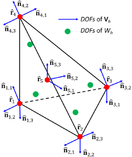
Figure 1: DOFs of $\mathbf{V}(\hat{E})$ and $W(\hat{E}$ for the case $d=3$.

We use the Piola transformation BBF to define the $RT_{1}$ velocity space in each simplex (e.g., W-Y ), as well as the standard change of variables for the pressure space:

$$\mathbf{v}\longleftrightarrow\mathbf{\hat{v}}:\mathbf{v}=\frac{1}{\left|\mathbf{J}_{E}\right|}\mathbf{J}_{E}\mathbf{\hat{v}},\quad\mathbf{J}_{E}=\left[\mathbf{r}_{21},\mathbf{r}_{31}\right]\ \textnormal{if}\ d=2,\quad\mathbf{J}_{E}=\left[\mathbf{r}_{21},\mathbf{r}_{31},\mathbf{r}_{41}\right]\ \textnormal{if}\ d=3,$$ (5.2a)

$$w\longleftrightarrow\hat{w}:w=\hat{w},$$ (5.2b)

where $\mathbf{J}_{E}$ is the Jacobian matrix associated with the mapping (5.1), and $\mathbf{r}_{ij}=\mathbf{r}_{i}-\mathbf{r}_{j}$. The determinant of $\mathbf{J}_{E}$ is $\left|\mathbf{J}_{E}\right|=2\left|E\right|$ with $\left|E\right|$ the area of simplex $E$, if $d=2$, or $\left|\mathbf{J}_{E}\right|=6\left|E\right|$ with $\left|E\right|$ the the volume of $E$, if $d=3$. Two important properties of the Piola transformation are BBF

$$\nabla\cdot\mathbf{v}=\frac{1}{\left|\mathbf{J}_{E}\right|}\nabla_{\hat{\mathbf{x}}}\cdot\mathbf{\hat{v}},\quad\mathbf{v}\cdot\mathbf{n}_{e}=\frac{\left|\hat{e}\right|}{\left|e\right|}\hat{\mathbf{v}}\cdot\hat{\mathbf{n}}_{e},$$

where $F_{E}:\hat{e}\to e$, $\mathbf{n}_{e}$ and $\hat{\mathbf{n}}_{e}$ are the unit normal vectors on the faces $e$ and $\hat{e}$, respectively, and $|e|$ is the length (if $d=2$) or area (if $d=3$) of $e$. Thanks to the property of the Piola transformation to preserve the vectors normal components, we get the continuity of $\mathbf{v}\cdot\mathbf{n}$ across any face $e$ BBF .

The $RT_{1}$ spaces on $T_{h}$ are defined as

$$\mathbf{V}_{h}=\left\{\mathbf{v}\in\mathbf{V}:\mathbf{v}|_{E}\longleftrightarrow\hat{\mathbf{v}},\ \hat{\mathbf{v}}\in\hat{\mathbf{V}}(\hat{E})\ \forall E\in T_{h}\right\},$$

$$W_{h}=\left\{w\in W:w|_{E}\longleftrightarrow\hat{w},\ \hat{w}\in\hat{W}(\hat{E})\ \forall E\in T_{h}\right\},$$

where (5.2) defines the the transformations $\mathbf{v}\longleftrightarrow\hat{\mathbf{v}}$ and $w\longleftrightarrow\hat{w}$.

Table 1: The $RT_{1}$ basis functions for the reference tetrahedron ($d=3$.) (see Radu )

$\hat{\mathbf{v}}_{1,1}$	$3\hat{x}+\hat{y}+\hat{z}-1-2\hat{x}^{2}-\hat{y}\hat{x}-\hat{z}\hat{x}$	$-2\hat{x}\hat{y}-\hat{y}^{2}+\hat{y}-\hat{z}\hat{y}$	$-2\hat{x}\hat{z}-\hat{z}\hat{y}-\hat{z}^{2}+\hat{z}$
$\hat{\mathbf{v}}_{1,2}$	$-\hat{x}^{2}+\hat{x}-2\hat{y}\hat{x}-\hat{z}\hat{x}$	$\hat{x}+3\hat{y}+\hat{z}-1-\hat{x}\hat{y}-2\hat{y}^{2}-\hat{z}\hat{y}$	$-\hat{x}\hat{z}-2\hat{z}\hat{y}-\hat{z}^{2}+\hat{z}$
$\hat{\mathbf{v}}_{1,3}$	$-\hat{x}^{2}+\hat{x}-\hat{y}\hat{x}-2\hat{z}\hat{x}$	$-\hat{x}\hat{y}-\hat{y}^{2}+\hat{y}-2\hat{z}\hat{y}$	$\hat{x}+\hat{y}+3\hat{z}-1-\hat{x}\hat{z}-\hat{z}\hat{y}-2\hat{z}^{2}$
$\hat{\mathbf{v}}_{2,1}$	$\hat{x}^{2}-\hat{y}\hat{x}$	$-\hat{x}+\hat{y}\hat{x}-\hat{y}^{2}+\hat{y}$	$\hat{z}\hat{x}-\hat{y}\hat{z}$
$\hat{\mathbf{v}}_{2,2}$	$\hat{x}^{2}-\hat{z}\hat{x}$	$\hat{y}\hat{x}-\hat{z}\hat{y}$	$-\hat{x}+\hat{z}\hat{x}-\hat{z}^{2}+\hat{z}$
$\hat{\mathbf{v}}_{2,3}$	$\sqrt{3}\left(2\hat{x}^{2}-\hat{x}+\hat{y}\hat{x}+\hat{z}\hat{x}\right)$	$\sqrt{3}\left(2\hat{x}\hat{y}+\hat{y}^{2}-\hat{y}+\hat{z}\hat{y}\right)$	$\sqrt{3}\left(2\hat{x}\hat{z}+\hat{z}\hat{y}+\hat{z}^{2}-\hat{z}\right)$
$\hat{\mathbf{v}}_{3,1}$	$\hat{x}\hat{y}-\hat{x}\hat{z}$	$\hat{y}^{2}-\hat{z}\hat{y}$	$-\hat{y}+\hat{y}\hat{z}-\hat{z}^{2}+\hat{z}$
$\hat{\mathbf{v}}_{3,2}$	$\sqrt{3}\left(\hat{x}^{2}-\hat{x}+2\hat{x}\hat{y}+\hat{x}\hat{z}\right)$	$\sqrt{3}\left(\hat{x}\hat{y}+2\hat{y}^{2}-\hat{y}+\hat{y}\hat{z}\right)$	$\sqrt{3}\left(\hat{x}\hat{z}+\hat{y}\hat{z}+\hat{z}^{2}-\hat{z}\right)$
$\hat{\mathbf{v}}_{3,3}$	$-\hat{y}-\hat{x}^{2}+\hat{x}+\hat{y}\hat{x}$	$\hat{y}-\hat{y}\hat{x}+\hat{y}^{2}-\hat{y}$	$-\hat{x}\hat{z}+\hat{y}\hat{z}$
$\hat{\mathbf{v}}_{4,1}$	$\sqrt{3}\left(\hat{x}^{2}-\hat{x}+\hat{y}\hat{x}+2\hat{z}\hat{x}\right)$	$\sqrt{3}\left(\hat{y}\hat{x}+\hat{y}^{2}-\hat{y}+2\hat{z}\hat{y}\right)$	$\sqrt{3}\left(\hat{z}\hat{x}+\hat{z}\hat{y}+2\hat{z}^{2}-\hat{z}\right)$
$\hat{\mathbf{v}}_{4,2}$	$-\hat{z}-\hat{x}^{2}+\hat{x}+\hat{z}\hat{x}$	$-\hat{y}\hat{x}+\hat{z}\hat{y}$	$-\hat{z}\hat{x}+\hat{z}^{2}$
$\hat{\mathbf{v}}_{4,3}$	$-\hat{y}\hat{z}+\hat{z}\hat{x}$	$-\hat{z}-\hat{y}^{2}+\hat{y}+\hat{y}\hat{z}$	$-\hat{z}\hat{y}+\hat{z}^{2}$
$\hat{\mathbf{v}}_{5,1}$	$-8\left(\hat{x}^{2}-\hat{x}\right)-4\left(\hat{x}\hat{y}\right)-4\left(\hat{x}\hat{z}\right)$	$-8\left(\hat{x}\hat{y}\right)-4\left(\hat{y}^{2}-\hat{y}\right)-4\left(\hat{y}\hat{z}\right)$	$-8\left(\hat{x}\hat{z}\right)-4\left(\hat{z}\hat{y}\right)-4\left(\hat{z}^{2}-\hat{z}\right)$
$\hat{\mathbf{v}}_{5,2}$	$-4\left(\hat{x}^{2}-\hat{x}\right)-8\left(\hat{x}\hat{y}\right)-4\left(\hat{x}\hat{z}\right)$	$-4\left(\hat{x}\hat{y}\right)-8\left(\hat{y}^{2}-\hat{y}\right)-4\left(\hat{y}\hat{z}\right)$	$-4\left(\hat{x}\hat{z}\right)-8\left(\hat{z}\hat{y}\right)-4\left(\hat{z}^{2}-\hat{z}\right)$
$\hat{\mathbf{v}}_{5,3}$	$-4\left(\hat{x}^{2}-\hat{x}\right)-4\left(\hat{x}\hat{y}\right)-8\left(\hat{x}\hat{z}\right)$	$-4\left(\hat{x}\hat{y}\right)-4\left(\hat{y}^{2}-\hat{y}\right)-8\left(\hat{y}\hat{z}\right)$	$-4\left(\hat{x}\hat{z}\right)-4\left(\hat{z}\hat{y}\right)-8\left(\hat{z}^{2}-\hat{z}\right)$

5.2 The quadrature rule

Let $\mathbf{s},\mathbf{v}$ be any pair of continuous vector functions. The following second order accurate quadrature rule is defined in Radu :

$$\left(\mathbf{s},\mathbf{v}\right)_{Q}=\sum_{E\in T_{h}}\left(\mathbf{s},\mathbf{v}\right)_{Q,E}=\sum_{E\in T_{h}}|E|\sum_{i=1}^{d+2}\omega_{i}\,\mathbf{s}\left(\mathbf{r}_{i}\right)\cdot\mathbf{v}\left(\mathbf{r}_{i}\right),$$ (5.3)

where the weights are $\omega_{i}=\frac{1}{\left(k+1\right)\times\left(k+2\right)}$, $i=1,\dots,d+1$, $\omega_{d+2}=\frac{d+1}{d+2}$. If $\mathbf{v}\in\mathbf{V}_{h}$, the vertex vector $\mathbf{v}(\mathbf{r}_{i})$, $i=1,\dots,d+1$, can be uniquely obtained from the DOFs $\mathbf{v}(\mathbf{r}_{i})\cdot\mathbf{n}_{i,1},\dots,\mathbf{v}(\mathbf{r}_{i})\cdot\mathbf{n}_{i,d}$, i.e., its normal components to the $d$ faces sharing vertex $\mathbf{r}_{i}$. In a similar way, the vector at the center of mass $\mathbf{r}_{d+2}$ can be constructed from the DOFs $\mathbf{v}(\mathbf{r}_{d+2})\cdot\mathbf{n}_{d+2,1},\dots,\mathbf{v}(\mathbf{r}_{d+2})\cdot\mathbf{n}_{d+2,d}$.

The quadrature rule (5.3) is applied to the bilinear forms $(\frac{\phi}{\nu}\bm{\sigma}_{h}^{n+1},\bm{\tau}_{h})$ in (3.9a) in the PP and $\left(\frac{\mathbf{u}_{h}^{n+1}-\tilde{\mathbf{u}}_{h}^{n+1}}{\Delta t},\mathbf{v}_{h}\right)+\Bigl(\mathbf{L}\left(\mathbf{u}_{h}^{n+1}-\tilde{\mathbf{u}}_{h}^{n+1}\right),\mathbf{v}_{h}\Bigr)$ in (3.11a) in the PjP. The quadrature rule couples only the $d$ basis functions associated with the quadrature vertex $\mathbf{r}_{i}$ W-Y , Radu . This implies that the viscous stress $\bm{\sigma}^{n+1}_{x\left(y,z\right),h}$ and the velocity $\mathbf{u}_{h}^{n+1}$ can be locally eliminated, resulting in spd systems for $\tilde{\mathbf{u}}_{x\left(y,z\right),h}^{n+1}$ in (3.9) and $\Psi_{h}^{n+1}$ in (3.11), respectively.

In the following sections, we describe our numerical methodology for a three dimensional computational domain $\Omega\subset\mathbf{R}^{d}$ with $d=3$.

5.3 Predictor Problem

The PP (3.9) is solved separately for the $x$, $y$ and $z$ stress and velocity components. We denote by $\bm{\sigma}_{x,h}^{n+1}$, $\bm{\sigma}_{y,h}^{n+1}$ and $\bm{\sigma}_{z,h}^{n+1}$ the first, second and third rows of tensor $\bm{\sigma}_{h}^{n+1}$, respectively, and by $\tilde{u}_{x,h}^{n+1}$, $\tilde{u}_{y,h}^{n+1}$ and $\tilde{u}_{z,h}^{n+1}$ the three components of $\tilde{\mathbf{u}}_{h}^{n+1}$. Similarly, $q_{x,h}^{n}$, $q_{y,h}^{n}$ and $q_{z,h}^{n}$ are the components of $\mathbf{q}_{h}^{n}$, while for the BCs we set $\bm{\Sigma}_{b}=(\Sigma_{x,b},\Sigma_{y,b},\Sigma_{z,b})^{T}$ and $\mathbf{u}_{b}=(u_{x,b},u_{y,b},u_{z,b})^{T}$. In the following, our method is presented only for the $x$-component, with similar formulations along the other directions.

Applying the quadrature rule (5.3), the $x$-component of the PP (3.9) becomes: find $\bm{\sigma}_{x,h}^{n+1}\in\mathbf{V}_{h}:\bm{\sigma}_{x,h}^{n+1}\cdot\mathbf{n}=Q_{h}^{\Gamma}(\Sigma_{x,b}^{n+1}-\Psi_{b}^{n}\ n_{x})$ on $\Gamma_{n}$ and $\tilde{u}_{x,h}^{n+1}\in W_{h}$, such that

$$\left(\frac{\phi}{\nu}\bm{\sigma}_{x,h}^{n+1},\bm{\tau}_{h}\right)_{Q}-\left(\tilde{u}_{x,h}^{n+1},\nabla\cdot\bm{\tau}_{h}\right)=-\langle u_{x,b}^{n+1},\bm{\tau}_{h}\cdot\mathbf{n}\rangle_{\Gamma_{d}}\quad\forall\bm{\tau}_{h}\in\mathbf{V}_{h,0,\Gamma_{n}},$$ (5.4a)

$$\left(\frac{1}{\phi}\frac{\tilde{u}_{x,h}^{n+1}-u_{x,h}^{n}}{\Delta t},\xi_{h}\right)+\left(\nabla\cdot\bm{\sigma}_{x,h}^{n+1},\xi_{h}\right)+\left(q_{x,h}^{n},\xi_{h}\right)$$

$$\quad+\left(\left(L_{11}\tilde{u}_{x,h}^{n+1}+L_{12}\tilde{u}_{y,h}^{n}+L_{13}\tilde{u}_{z,h}^{n}\right),\xi_{h}\right)=0\quad\forall\xi_{h}\in W_{h}.$$ (5.4b)

where $L_{ij}$, $i,j=1,2,3$, are the coefficients of tensor $\mathbf{L}$ defined in (3.1). We note that the $y$- and $z$-components $\tilde{u}_{y,h}$ and $\tilde{u}_{z,h}$ in the last term are evaluated at the previous time $t^{n}$, which allows for complete decoupling of the problems for each component. Next, the local elimination of the viscous stress $\bm{\sigma}_{x,h}^{n+1}$ is described both for the case of any internal or boundary vertex and the center of mass midpoint of any simplex.

The case of any vertex. Let $\mathbf{r}$ be any internal vertex of $T_{h}$ shared by $\mathcal{I}$ interfaces and $\mathcal{I}$ simplices, denoted by $e_{i}$ and $E_{i}$, respectively. Let $\bm{\tau}_{i}\in\mathbf{V}_{h}$ be the basis functions on the faces $e_{i}$, and $\sigma_{x,i}^{n+1}$ be the associated DOFs of $\bm{\sigma}^{n+1}_{x,h}$. Thanks to the property of the quadrature rule to localize the interaction of the face DOFs, setting $\bm{\tau}_{h}=\bm{\tau}_{1},\ldots,\bm{\tau}_{\mathcal{I}}$ in (5.4a) results in a $\left(\mathcal{I}\times\mathcal{I}\right)$ local linear system for the $\sigma^{n+1}_{{x,i}}$ unknowns, $i=1,\dots,\mathcal{I}$:

$$\sum_{j}\sigma^{n+1}_{x,j}\left(\left(\frac{\phi}{\nu}\bm{\tau}_{j},\bm{\tau}_{i}\right)_{Q,E_{a}}+\left(\frac{\phi}{\nu}\bm{\tau}_{j},\bm{\tau}_{i}\right)_{Q,E_{b}}\right)=(\tilde{u}^{n+1}_{x,h},\nabla\cdot\bm{\tau}_{i})_{E_{a}}+(\tilde{u}^{n+1}_{x,h},\nabla\cdot\bm{\tau}_{i})_{E_{b}},\ i=1,\dots,\mathcal{I},$$ (5.5)

where $E_{a}$ and $E_{b}$ are the two simplices sharing face $e_{i}$ and the summation on $j$ on the l.h.s. is over the faces $e_{j}\left(\in E_{a}\cup E_{b}\right)$ sharing with $e_{i}$ the vertex associated with $\bm{\tau}_{i}$. The integrals $(\tilde{u}^{n+1}_{x,h},\nabla\cdot\bm{\tau}_{h})_{E_{a(b)}}$ on the r.h.s. by computed by a $\left(d+1\right)$-point Gaussian integration rule. This quadrature rule is exact for quadratic functions, and since both $\tilde{u}^{n+1}_{x,h}\in P_{1}\left(E\right)$ and $\nabla\cdot\bm{\tau}_{h}\in P_{1}\left(E\right)$, it is exact for $(\tilde{u}^{n+1}_{x,h},\nabla\cdot\bm{\tau}_{h})_{E_{a(b)}}$.

The matrix-vector form of the local linear system (5.5) is

$$\mathbf{A}\mathbf{\Sigma}_{x}=\mathbf{B}^{T}\mathbf{U}_{x},$$ (5.6)

where

• $\mathbf{A}$ is a $\left(\mathcal{I}\times\mathcal{I}\right)$ matrix with coefficients $A_{ij}=\left(\frac{\phi}{\nu}\bm{\tau}_{j},\bm{\tau}_{i}\right)_{Q}$, $i,j=1,\ldots,\mathcal{I}$,

• $\mathbf{\Sigma}_{x}$ is a $\left(\mathcal{I}\times 1\right)$ vector whose coefficients are the DOFs $\sigma^{n+1}_{x,i}$, $i=1,\dots,\mathcal{I}$,

• $\mathbf{B}^{T}$ is a $\left(\mathcal{I}\times\left(\left(d+1\right)\times\mathcal{I}\right)\right)$ matrix with coefficients coming from $(\tilde{u}^{n+1}_{x,h},\nabla\cdot\bm{\tau}_{i})_{E_{a}}$ + $(\tilde{u}^{n+1}_{x,h},\nabla\cdot\bm{\tau}_{i})_{E_{b}}$, $i=1,\ldots,\mathcal{I}$,

• $\mathbf{U}_{x}$ is a $\left(\left(\left(d+1\right)\times\mathcal{I}\right)\times 1\right)$ vector, whose coefficients are the $\left(d+1\right)$ DOFs of $\tilde{u}^{n+1}_{x,h}$ within each simplex $E_{i}$, $i=1,\ldots,\mathcal{I}$.

The matrix $\mathbf{A}$ is spd  as proved in W-Y , which implies that the local system (5.6) is solvable and one can express the $\mathcal{I}$ DOFs $\sigma^{n+1}_{x,i}$, $i=1,\dots,\mathcal{I}$, sharing vertex $\mathbf{r}$ in terms of the $\left(\left(d+1\right)\times\mathcal{I}\right)$ DOFs of $\tilde{u}^{n+1}_{x,h}$ on the $\mathcal{I}$ simplices sharing $\mathbf{r}$.

Let $\mathbf{r}$ be a boundary vertex and denote by $\mathcal{I}$ and $\mathcal{H}$ the number of interfaces and simplices sharing $\mathbf{r}$, respectively, where generally $\mathcal{I}\neq\mathcal{H}$. In this case the size of matrix $\mathbf{B}^{T}$ is $\left(\mathcal{I}\times\left(\left(d+1\right)\times(\mathcal{H}\right))\right)$ and the size of vector $\breve{\mathbf{U}}_{x}$ is $\left(\left(d+1\right)\times(\mathcal{H})\times 1\right)$. If $\mathbf{r}\in\overline{\Gamma}_{d}$, thanks to (5.4a), we also account for the contribution $-\langle u^{n+1}_{x,b},\bm{\tau}_{h}\cdot\mathbf{n}\rangle_{\Gamma_{d}}$ in the local system (5.6), computed by numerical integration over the face(s) $e_{i}\in\Gamma_{d}$ sharing $\mathbf{r}$. The system (5.4) changes as

$$\mathbf{A}\mathbf{\Sigma}_{x}=\mathbf{B}^{T}\mathbf{U}_{x}+\mathbf{G}_{d,x},$$ (5.7)

where the size of vector $\mathbf{G}_{d,x}$ is $\left(\mathcal{I}\times 1\right)$ and its nonzero coefficients appear only in the rows associated with the boundary faces $e_{i}\in\Gamma_{d}$ sharing $\mathbf{r}$. If $\mathbf{r}\in\overline{\Gamma}_{n}$, the local system (5.4) incorporates the essential stress boundary condition:

$$\tilde{\mathbf{A}}\mathbf{\Sigma}_{x}=\tilde{\mathbf{B}}^{T}\mathbf{U}_{x}+\mathbf{G}_{n,x},$$ (5.8)

where $\mathbf{G}_{n,x}$ is a $\left(\mathcal{I}\times 1\right)$ vector.

The case of any center of mass. Let $\mathbf{r}$ be the center of mass of any simplex $E$ and let $\bm{\tau}_{i}\in\mathbf{V}_{h}$, $i=1,\dots,d$, be the associated stress basis functions. Let $\sigma^{n+1}_{x,i}$ be the $d$ DOFs of $\bm{\sigma}^{n+1}_{x,h}$ associated with $\mathbf{r}$. Since the quadrature rule localizes the interaction of DOFs, $\sigma^{n+1}_{x,i}$, $i=1,\dots,d$ are coupled only with each other, resulting in a $d\times d$ linear system with spd matrix written in the same form as in (5.6) for $\sigma^{n+1}_{x,i}$, $i=1,\dots,d$.

The PP solved for $\tilde{\mathbf{u}}^{n+1}$ velocity component. With the local elimination of the viscous stress, as previously described, the MFMFE scheme of the PP becomes a system for the $\tilde{u}_{x,h}^{n+1}$ with $\left(d+1\right)$ DOFs per simplex, and the associated algebraic system arising from (5.4) becomes

$$\begin{pmatrix}\mathrm{A}\quad-\mathrm{B}^{T}\\ \mathrm{B}\ \qquad\mathrm{D}\end{pmatrix}\begin{pmatrix}\mathrm{\Sigma}_{x}\\ \mathrm{U}_{x}\end{pmatrix}=\begin{pmatrix}\mathrm{G}_{x}\\ \mathrm{Q}_{x}+\mathrm{F}_{x}+\mathrm{L}_{y}+\mathrm{L}_{z}\end{pmatrix},$$ (5.9)

where

• $\mathrm{A}$ is a $\left(\mathfrak{I}\times\mathfrak{I}\right)$ block diagonal matrix, with $\mathfrak{I}=d\times\mathfrak{S}_{T}+d\times N_{T}$, (with $\mathfrak{S}_{T}$ and $N_{T}$ the total number of the faces and simplices, respectively, as specified in Section˜3.1). Matrix $\mathrm{A}$ is given by assembling the (local) block matrices $\mathbf{A}$, cf. (5.6),

• $\mathrm{\Sigma}_{x}$ is a $\left(\mathfrak{I}\times 1\right)$ vector whose coefficients are the DOFs of $\bm{\sigma}_{x,h}^{n+1}$, obtained by assembling the (local) vectors $\mathbf{\Sigma}_{x}$, cf. (5.6),

• $\mathrm{B}^{T}$ is a $\left(\mathfrak{I}\times\left(d\times N_{T}\right)\right)$ matrix, obtained by assembling the block (local) matrices $\mathbf{B}^{T}$, cf. Eq.˜5.6,

• $\mathrm{D}$ is a $\left(\left(d\times N_{T}\right)\times\left(d\times N_{T}\right)\right)$ block diagonal matrix, whose blocks are associated with $\left(\left(\frac{1}{\phi}\frac{1}{\Delta t}+L_{{11}}\right)\tilde{u}_{x,h}^{n+1},\xi_{h}\right)$ in (5.4),

• $\mathrm{U}_{x}$ is a $\left(\left(d\times N_{T}\right)\times 1\right)$ vector, with coefficients the DOFs of $\tilde{u}_{x,h}^{n+1}$,

• $\mathrm{G}_{x}$ is a $\left(\mathfrak{I}\times 1\right)$ vector obtained by the assembly of the local vectors $\mathbf{G}_{d,x}$ and $\mathbf{G}_{n,x}$,

• $\mathrm{Q}_{x}$, $\mathrm{F}_{x}$, $\mathrm{L}_{y}$ and $\mathrm{L}_{z}$ are $\left(\left(d\times N_{T}\right)\times 1\right)$ vectors corresponding to $-\left(q_{x,h}^{n},\xi_{h}\right)$, $\left(\frac{1}{\phi}\frac{1}{\Delta t}u_{x,h}^{n},\xi_{h}\right)$, $\left(L_{{12}}u_{y,h}^{n},\xi_{h}\right)$ and $\left(L_{{13}}u_{z,h}^{n},\xi_{h}\right)$ in (5.4), respectively.

Similar to $\mathrm{B}$, the integrals in $\mathrm{D}$, $\mathrm{Q}_{x}$, $\mathrm{F}_{x}$, $\mathrm{L}_{y}$ and $\mathrm{L}_{z}$ are computed by a $\left(d+1\right)$-point Gaussian quadrature rule

By inverting the matrix $\mathrm{A}$, the unknown stress vector $\mathrm{\Sigma}_{x}$ can be eliminated in Eq.˜5.9, resulting in a $\left(\left(\left(d+1\right)\times N_{T}\right)\times\left(\left(d+1\right)\times N_{T}\right)\right)$ system for $\mathrm{U}_{x}$:

$$\left(\mathrm{D}+\mathrm{B}\ \mathrm{A}^{-1}\ \mathrm{B}^{T}\right)\mathrm{U}_{x}=\mathrm{Q}_{x}+\mathrm{F}_{x}+\mathrm{L}_{y}+\mathrm{L}_{z}+\mathrm{B}\mathrm{A}^{-1}\mathrm{G}_{x},$$ (5.10)

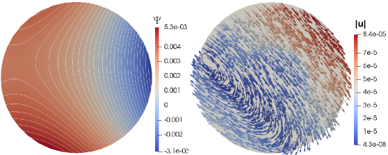
Figure 3: Test 1. Computed solution 1st refinement grid level, case 1. $\Psi$ (left), $\mathbf{u}$ (right)

where the $\left(d+1\right)$ DOFs of $\tilde{u}^{n+1}_{x,h}$ within each simplex $E$ are coupled with the $\left(d+1\right)$ DOFs of all simplices sharing a vertex with $E$, see [ARICO2025117616, , Figure 3] for a 2D view.

The matrix in (5.10) is spd W-Y and the system is solved by a preconditioned conjugate gradient method with incomplete Cholesky factorization Dongarra , which results in a very fast and efficient procedure. A lot of computational effort is saved because the factorization of the matrix of system in (5.10) occurs only once, before the the time loop, since the matrix coefficients depend only on geometric quantities, the kinematic viscosity $\nu$, the time step size $\Delta t$, as well as the physical properties of the porous medium, like the porosity $\phi$ and the coefficients of the permeability tensor.

Remark 5.1.

With the ratio $\frac{\nu}{\phi}$ inside the divergence operator in (2.1b), we obtain a symmetric matrix in (5.10). It can be easily seen that this matrix would be non-symmetric if $\frac{\nu}{\phi}$ was outside the divergence operator.

We apply the same procedure along the $y$ and $z$ directions, with the system having the same matrix as in (5.10). At the end of the PP we obtain an intermediate velocity $\tilde{\mathbf{u}}^{n+1}_{h}|_{E}\in(P_{1}(E))^{2}$ and discontinuous, i.e., the continuity of normal flux at the simplex interfaces is not imposed in this step.

5.4 Projection problem and pressure gradient update

Applying the quadrature rule in (5.3), the PjP in (3.11) is: find $\mathbf{u}_{h}^{n+1}\in\mathbf{V}_{h}:\mathbf{u}_{h}^{n+1}\cdot\mathbf{n}=Q_{h}^{\Gamma}\left(\mathbf{u}_{b}\cdot\mathbf{n}\right)$ on $\Gamma_{d}$ and $\Psi_{h}^{n+1}\in W_{h}$ such that

$$\thinspace\bigg(\frac{1}{\phi}\frac{\mathbf{u}_{h}^{n+1}-\tilde{\mathbf{u}}_{h}^{n+1}}{\Delta t}+\mathbf{L}\left(\mathbf{u}_{h}^{n+1}-\tilde{\mathbf{u}}_{h}^{n+1}\right),\mathbf{v}_{h}\bigg)_{Q}-(\Psi_{h}^{n+1}-\Psi_{h}^{n},\nabla\cdot\mathbf{v}_{h})=$$

$$\quad-\langle\Psi_{b}^{n+1}-\Psi_{b}^{n},\mathbf{v}_{h}\cdot\mathbf{n}\rangle_{\Gamma_{n}}\ \forall\mathbf{v}_{h}\in\mathbf{V}_{h,0,\Gamma_{d}},$$ (5.11a)

$$\thinspace\left(\nabla\cdot\mathbf{u}_{h}^{n+1},w_{h}\right)=0\quad\forall w_{h}\in W_{h}.$$ (5.11b)

The method is the same as the one applied for the solution of the PP for $\bm{\sigma}_{x,h}^{n+1}\in\mathbf{V}_{h}$ and $\tilde{u}_{x,h}^{n+1}\in W_{h}$ in (5.4). The corrected velocity $\mathbf{u}_{h}^{n+1}$ is locally eliminated according to the same procedure as described in Section˜5.3, and we solve a spd system for $\Psi_{h}^{n+1}$ of type (5.10), where the $\left(d+1\right)$ DOFs of $\Psi_{h}^{n+1}$ within each simplex $E$ are coupled with the $\left(d+1\right)$ DOFs of those simplices sharing a vertex with $E$. The corrected velocity $\mathbf{u}_{h}^{n+1}$ can be easily recovered after the solution of the system by a local post-processing.

The term $\langle\Psi_{b}^{n+1}-\Psi_{b}^{n},\mathbf{v}_{h}\cdot\mathbf{n}\rangle_{\Gamma_{n}}$ in (5.11a) is computed via numerical integration using the boundary values of $\Psi_{b}^{n+1}$ on $\Gamma_{n}$ given by

$$\Psi_{b}^{n+1}|_{e}=\left(\bm{\Sigma}_{b}^{n+1}|_{e}+\left.\left(\frac{\nu}{\phi}\nabla\tilde{\mathbf{u}}_{h}^{n+1}\right)\right|_{e}\,\mathbf{n}\right)\cdot\mathbf{n},$$

where the tensor $\nabla\tilde{\mathbf{u}}_{h}^{n+1}$ is computed on the simplex $E$ with face $e$ and it has a constant value, since $\tilde{\mathbf{u}}_{h}^{n+1}\in(P_{1}(E))^{2}$.

Before the next time iteration, we update the pressure gradient according to (3.12). This is performed by updating the DOFs of $\mathbf{q}_{h}^{n+1}$, since both $\mathbf{q}_{h}^{n+1}$ and the test function $\bm{\xi}_{h}$ live in the same discretized space $(W_{h})^{d}$. For any degree of freedom point $\mathbf{r}$, we have

$$\mathbf{q}_{h}^{n+1}(\mathbf{r})=\mathbf{q}_{h}^{n}(\mathbf{r})-\left(\frac{1}{\Delta t}\frac{1}{\phi(\mathbf{r})}\mathbf{I}+\mathbf{L}(\mathbf{r})\right)\left(\mathbf{u}_{h}^{n+1}(\mathbf{r})-\tilde{\mathbf{u}}_{h}^{n+1}(\mathbf{r})\right).$$

6 Numerical Tests

In this section we present several numerical tests to illustrate the performance of the numerical method. We call “method 1” and “method 2” the standard method in (3.9)–(3.12) and the simplified method without the permeability correction term described in (4.15)–(4.16), respectively.

We present four numerical tests. Test 1 is devoted to the numerical investigation of the convergence order in space and time, both for $d=2$ and $d=3$. In Test 2 we study the flow of a free fluid around a porous obstacle under different working conditions and we also compare the results from methods 1 and 2. In Test 3 we consider the interaction of a free fluid with a porous region with a steps-like interface. For Tests 2 and 3, we compare the results of our method to numerical solutions available in the literature. Finally, Test 4 is a show-case application where we investigate the effect of a porous medium filling the aneurysmatic sac of a real-case intracranial aneurysm (ICA). We emphasize that tests 2-4 involve two regions with parameters in either the Stokes or Darcy regimes. The results illustrate the robustness of the proposed method in both regimes.

The computational grids of the applications proposed in this Section have been generated by the open-source software Netgen Schberl1997NETGENAA , the numerical scheme has been implemented in an in-house Fortran 90-95 code, and the the open-source software Paraview Paraview has been used for the post-processing and visualization of the results.

6.1 Test 1: study of the convergence order in space and time

The strategy we adopt to investigate the convergence order in space and time is

• consider a computational heterogeneous porous domain $\Omega\subset\mathbf{R}^{d}$, $d=2,3$, with assigned spatial distribution of porosity and permeability tensor coefficients,

• assign an analytical time-dependent solution for the velocity components $u_{x},u_{y},u_{z}$ and kinematic pressure $\Psi$, and the corresponding ICs and BCs,

• discretize $\Omega$ by a coarse simplicial grid $T_{h}$ and progressively operate some refinements of $T_{h}$,

To study the convergence order in space, we adopt a small enough time step size $\Delta t$ and compute the $L_{2}$-norms of the errors of $u_{x},u_{y},u_{z}$ and $\Psi$ as

$$L_{2}^{q}=\max_{1\leq n\leq N}\|q(t_{n})-q_{h}^{n}\|,\textnormal{ with }q=u_{x},\,u_{y},\,u_{z},\,\Psi,$$ (6.1)

where $N$ is the number of intervals in the time discretization, as specified in Section˜3.1.

If $h_{l}$ marks the grid size associated with the $l$-th refinement level and $e_{l}^{q}\sim h_{l}^{r_{h}^{q}}$ is the error of the variable $q$ in this level, we compute the the associated convergence rate $r_{h}^{q}$ by comparing the errors associated with two consecutive grid refinement levels with size $h_{l-1}$ and $h_{l}$:

$$r_{h}^{q}=\frac{\log\left(\frac{e_{l-1}^{q}}{e_{l}^{q}}\right)}{\log\left(\frac{h_{l-1}}{h_{l}}\right)}.$$ (6.2)

To investigate the convergence order in time, we run simulations over a refined enough grid, changing the time step size in a given range, and compute the $L_{2}$-norms of the errors as in (6.1). The rate of convergence in time is obtained as

$$r_{\Delta t}^{q}=\frac{\log\left(\frac{e_{l-1}^{q}}{e_{l}^{q}}\right)}{\log\left(\frac{\Delta t_{l-1}}{\Delta t_{l}}\right)},$$ (6.3)

where $\Delta t_{l-1}$ and $\Delta t_{l}$ are two consecutive time step sizes in the given range.

In the following 2D and 3D applications, we assume that the kinematic fluid viscosity is $\nu=1$.

6.1.1 2D study

We consider the circular domain $\Omega\subset\mathbf{R}^{2}$ shown in Fig.˜2(a) (top), where we have three layers (zones) with outer (dimensionless) radii 0.3, 0.5 and 1, respectively. Zones 1 and 2 are the inner and outer bulk porous regions, with constant in space values of the porosity $\phi$ and the permeability tensor $\mathbf{K}$ given as

$$\mathbf{K}=\mathbf{M}\mathbf{C}\mathbf{M}^{-1},\qquad\mathbf{M}=\begin{pmatrix}\cos\alpha&-\sin\alpha\\ \sin\alpha&\cos\alpha\end{pmatrix},\qquad\mathbf{C}=\begin{pmatrix}\frac{k}{\beta}&0\\ 0&k\end{pmatrix},$$ (6.4)

where $k$ and $\beta$ are positive scalar parameters and $\alpha$ is the anisotropy angle. The porosity and permeability parameters are listed in Table˜2. A transition layer (or zone), is located in between the two bulk regions (zone 3 in Fig.˜2(a) (top)). Here the values of $\phi$ and $\mathfrak{K}_{i,j}$ undergo continuous changes, from the values in zone 1 to the values in zone 2, according to

$$\phi\left(d\right)=\frac{1}{2}\left(\phi_{max}-\phi_{min}\right)\mbox{tanh}\left(d\,\theta_{\psi}\right)+\frac{1}{2}\left(\phi_{max}+\phi_{min}\right),$$ (6.5a)

$$\mathfrak{K}_{i,j}\left(d\right)=\mathfrak{K}^{0}_{i,j}\frac{1}{2}\left(1-\mbox{tanh}\left(d\,\theta_{\mathfrak{K}}\right)\right),$$ (6.5b)

which are similar to [Arico-ODA, , Eq. (39)]. In (6.5), $d$ is the distance from any point to the mid-line of the transition zone, assumed to be positive or negative depending on whether the point is in the side of zone 1 or 2, respectively. In addition, $\phi_{max}$ and $\phi_{min}$, as well as $\mathfrak{K}^{0}_{i,j}$, $i,j=1,\dots,d$, are positive real scalar parameters such that the porosity and permeability values in the transition layer and in the bulk porous regions match at the interfaces. The parameters $\theta_{\psi}$ and $\theta_{\mathfrak{K}}$ adjust the slope of the profiles. The values of all parameters are listed in Table˜3.

We assign the time-dependent (dimensionless) analytical solution

$$\Psi=\left(a_{1}+b_{1}x+c_{1}x^{2}+a_{2}+b_{2}y+c_{2}y^{2}\right)\cos\omega t,\quad\mathbf{u}=-\mathbf{K}\nabla\Psi,$$ (6.6)

where $a_{i},\ b_{i},\ c_{i}$ and $\omega$ are scalar real variables listed in Table˜4. We add source terms in the model equations (2.1) according to the assigned analytical solution. The maximum value of the Reynolds number is $Re=\frac{\|\mathbf{u}\|_{max}\ 2\ R_{out}}{\nu}\simeq 1.4\cdot 10^{-04}$, where $\|\mathbf{u}\|_{max}$ is the maximum value of the velocity magnitude and $R_{out}$ is the outer radius of the domain.

We discretize the domain by either a coarse regular grid or a distorted grid shown in Fig.˜2(a) (top) and denoted as $T_{h,R}$ and $T_{h,D}$, respectively. The number of triangles and vertices of $T_{h,R}$ and $T_{h,D}$ is 638 and 292, and 340 and 163, respectively. For any triangle $E\in T_{h,R}\textnormal{ or }E\in T_{h,D}$, we compute the dimensionless aspect ratio $A_{r}$,

$$A_{r}=\frac{2\ h_{n}}{\sqrt{3}\ L_{x}},$$ (6.7)

which represents the ratio between the aspect ratio of $E$, where $h_{n}$ and $L_{x}$ are the minimum and the maximum values of the heights and length sides of $E$, respectively, and the ideal aspect ratio of the equilateral triangle, $\frac{\sqrt{3}}{2}$. The minimum values of $A_{r}$ are approximately 0.53 and 0.33 for $T_{h,R}$ and $T_{h,D}$, respectively.

We perform five refinements of both $T_{h,R}$ and $T_{h,D}$, by halving each side. We consider two scenarios of the assigned BCs, depending on the distribution of the boundary portions $\Gamma_{d}$ and $\Gamma_{n}$, as in Fig.˜2(a) (bottom), denoted as “case 1” and “case 2”, respectively. The BCs in case 2 is a way we implement full Dirichlet boundary condition for the velocity, assigning $\Psi$ only at one edge in $\Gamma_{n}$ for the solution to be unique.

The ICs are obtained by Eq.˜6.6 by setting $t=0$. In Fig.˜3 we plot the computed solution over the 2nd refinement grid level and case 1 at the (dimensionless) simulation time $\mathcal{T}=2$.

To investigate the convergence order in space, we use a (dimensionless) time step size $\Delta t=1\cdot 10^{-04}$. The final (dimensionless) simulation time is $\mathcal{T}=6$. Tables 5–8 list the $L_{2}$-norms of the errors for the velocity components and pressure, as specified in (6.1), as well as the associated convergence order $r_{h}^{q}$, given by (6.2), for the two BCs cases and two grid choices. The convergence rate $r_{h}$ is approximately 2 in all tables. The values of $L_{2}^{u_{x(y)}}$ computed for the second BCs case are generally smaller than in the first BCs scenario, while the opposite occurs for $L_{2}^{\Psi}$. The errors computed over the sets of the regular grids are approximately a magnitude order smaller than the errors obtained over the sets of the distorted grids.

We investigate the convergence order in time running our simulations over the $3^{rd}$ refined grid level and using a (dimensionless) time step size $\Delta t$ in the range $\left[1\cdot 10^{-04},1\cdot 10^{-01}\right]$. Tables 9–12 list the computed $L_{2}$-norms of the errors and the associated convergence order $r_{\Delta t}^{q}$. The rate $r_{\Delta t}^{q}$ is approximately 1, in line with the theoretically proved first order in Theorem˜4.3.

We have also studied the convergence order in space and time for method 2. For sake of space, we present only the errors and rates over the set of distorted grids for the second BCs case in Tables˜13 and 14, observing again second order in space and first order in time. We note that the errors for the two methods are similar in this test with smooth analytical solution. However, in Test 2 we illustrate that method 2 may produce less accurate results that method 1 for more challenging problems.

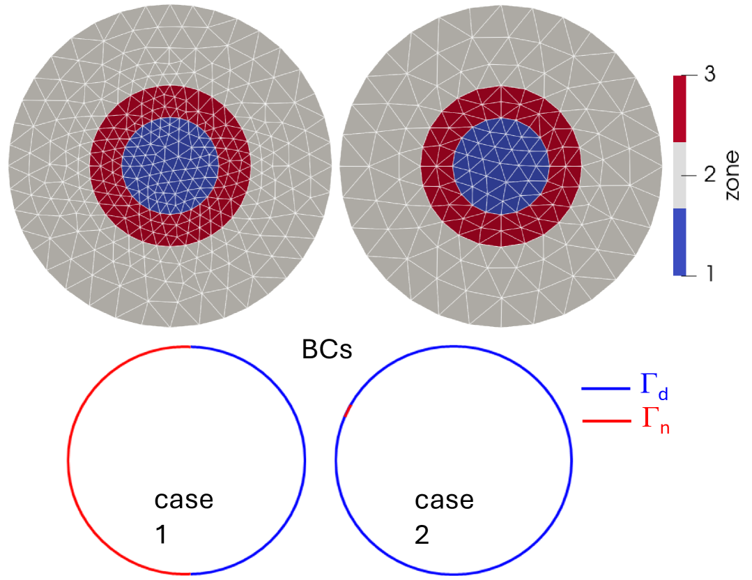
(a) Test 1, 2D case. Top: coarse grids $T_{h,R}$ (left) and $T_{h,D}$ (right) and porous medium zones (the color bar indicates the zone number). Bottom: assigned BCs.

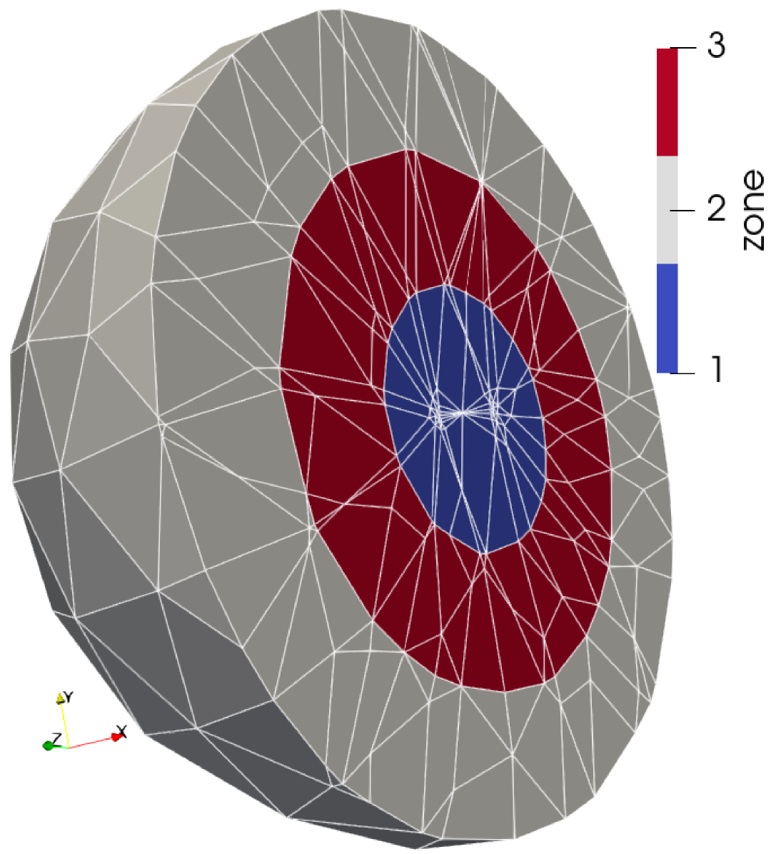
(b) Test 1, 3D case. Porous medium zones (the color bar indicates the zone number).

Figure 2: Test 1, 2D and 3D cases.

Table 2: Test 1, 2D case. (Dimensionless) parameters of the bulk porous regions.

zone	$\phi$	$\alpha$	$\beta$	$k$	$\mathfrak{K}_{1,1}$	$\mathfrak{K}_{2,2}$	$\mathfrak{K}_{1,2}=\mathfrak{K}_{2,1}$
1	0.597	$-\pi/4$	10	$1.37\cdot 10^{02}$	403	403	-329
2	0.7037	$-\pi/4$	10	$3.72\cdot 10^{02}$	147.9	147.9	-121

Table 3: Test 1, 2D case. (Dimensionless) parameters of the transition porous zone.

zone	$\phi_{max}$	$\phi_{min}$	$\theta_{\psi}$	$\theta_{\mathfrak{K}_{i,j}}$	$\mathfrak{K}^{0}_{1,1}$	$\mathfrak{K}^{0}_{2,2}$	$\mathfrak{K}^{0}_{1,2}=\mathfrak{K}^{0}_{2,1}$
3	0.766	0.5344	5	5	550	550	-450

Table 4: Test 1, 2D case. (Dimensionless) parameters of the assigned analytical solution in (6.5).

$a_{1}$	$b_{1}$	$c_{1}$	$a_{2}$	$b_{2}$	$c_{2}$	$\omega$
$5\cdot 10^{-04}$	$1.5\cdot 10^{-03}$	$-3.2\cdot 10^{-03}$	$-8\cdot 10^{-04}$	$-1.95\cdot 10^{-03}$	$1.95\cdot 10^{-03}$	$\pi$

Table 5: Test 1, 2D case, method 1. $L_{2}$-norms of errors and rates in space: $T_{h,R}$, BCs case 1.

ref. level $l$	$L_{2}^{u_{x}}$	$L_{2}^{u_{y}}$	$L_{2}^{\Psi}$	$r_{h}^{u_{x}}$	$r_{h}^{u_{y}}$	$r_{h}^{\Psi}$
0	$5.51\cdot 10^{-04}$	$5.51\cdot 10^{-04}$	$9.24\cdot 10^{-02}$
1	$1.33\cdot 10^{-04}$	$1.47\cdot 10^{-04}$	$1.72\cdot 10^{-02}$	2.05	1.9	2.42
2	$3.3\cdot 10^{-05}$	$3.45\cdot 10^{-05}$	$4.15\cdot 10^{-03}$	2.01	2.1	2.05
3	$7.9\cdot 10^{-06}$	$8.16\cdot 10^{-06}$	$1.4\cdot 10^{-03}$	2.06	2.08	2
4	$1.88\cdot 10^{-06}$	$1.98\cdot 10^{-06}$	$2.57\cdot 10^{-04}$	2.07	2.05	2.01
5	$4.69\cdot 10^{-07}$	$4.81\cdot 10^{-07}$	$6.4\cdot 10^{-05}$	2	2.04	2.01

Table 6: Test 1, 2D case, method 1. $L_{2}$-norms of errors and rates in space: $T_{h,R}$, BCs case 2.

ref. level $l$	$L_{2}^{u_{x}}$	$L_{2}^{u_{y}}$	$L_{2}^{\Psi}$	$r_{h}^{u_{x}}$	$r_{h}^{u_{y}}$	$r_{h}^{\Psi}$
0	$8.39\cdot 10^{-04}$	$8.05\cdot 10^{-04}$	$1.38\cdot 10^{-02}$
1	$1.18\cdot 10^{-04}$	$1.16\cdot 10^{-04}$	$3.11\cdot 10^{-02}$	2.83	2.79	2.15
2	$2.02\cdot 10^{-05}$	$2.13\cdot 10^{-05}$	$7.7\cdot 10^{-03}$	2.55	2.45	2.01
3	$4.32\cdot 10^{-06}$	$4.76\cdot 10^{-06}$	$1.91\cdot 10^{-03}$	2.22	2.16	2.01
4	$1\cdot 10^{-06}$	$1.1\cdot 10^{-06}$	$4.78\cdot 10^{-04}$	2.11	2.11	2
5	$2.43\cdot 10^{-07}$	$2.59\cdot 10^{-07}$	$1.21\cdot 10^{-04}$	2.04	2.09	1.99

Table 7: Test 1, 2D case, method 1. $L_{2}$-norms of errors and rates in space: $T_{h,D}$, BCs case 1.

ref. level $l$	$L_{2}^{u_{x}}$	$L_{2}^{u_{y}}$	$L_{2}^{\Psi}$	$r_{h}^{u_{x}}$	$r_{h}^{u_{y}}$	$r_{h}^{\Psi}$
0	$3.06\cdot 10^{-03}$	$2.64\cdot 10^{-03}$	$3.4\cdot 10^{-01}$
1	$4.39\cdot 10^{-04}$	$3.81\cdot 10^{-04}$	$7.7\cdot 10^{-02}$	2.8	2.8	2.14
2	$1.02\cdot 10^{-04}$	$8.79\cdot 10^{-05}$	$1.88\cdot 10^{-02}$	2.1	2.12	2.04
3	$2.4\cdot 10^{-05}$	$2.04\cdot 10^{-05}$	$4.5\cdot 10^{-03}$	2.09	2.11	2.06
4	$5.6\cdot 10^{-06}$	$4.99\cdot 10^{-06}$	$1.12\cdot 10^{-03}$	2.1	2.03	2.01
5	$1.35\cdot 10^{-06}$	$1.24\cdot 10^{-06}$	$2.8\cdot 10^{-04}$	2.05	2.01	2

Table 8: Test 1, 2D case, method 1. $L_{2}$-norms of errors and rates in space: $T_{h,D}$, BCs case 2.

ref. level $l$	$L_{2}^{u_{x}}$	$L_{2}^{u_{y}}$	$L_{2}^{\Psi}$	$r_{h}^{u_{x}}$	$r_{h}^{u_{y}}$	$r_{h}^{\Psi}$
0	$6.07\cdot 10^{-03}$	$7\cdot 10^{-03}$	$7.1\cdot 10^{-01}$
1	$8.01\cdot 10^{-04}$	$9.09\cdot 10^{-04}$	$1.6\cdot 10^{-01}$	2.92	2.95	2.15
2	$1.08\cdot 10^{-04}$	$1.2\cdot 10^{-04}$	$4\cdot 10^{-02}$	2.89	2.92	2
3	$2.06\cdot 10^{-05}$	$2.08\cdot 10^{-05}$	$9.98\cdot 10^{-03}$	2.39	2.53	2
4	$4.79\cdot 10^{-06}$	$4.9\cdot 10^{-06}$	$2.48\cdot 10^{-03}$	2.1	2.09	2.01
5	$1.19\cdot 10^{-06}$	$1.17\cdot 10^{-06}$	$6.24\cdot 10^{-04}$	2.01	2.06	1.99

Table 9: Test 1, 2D case, method 1. $L_{2}$-norms of errors and rates in time: $T_{h,R}$, BCs case 1.

$\Delta t$	$L_{2}^{u_{x}}$	$L_{2}^{u_{y}}$	$L_{2}^{\Psi}$	$r_{\Delta t}^{u_{x}}$	$r_{\Delta t}^{u_{y}}$	$r_{\Delta t}^{\Psi}$
$1\cdot 10^{01}$	$8.2\cdot 10^{-03}$	$8.4\cdot 10^{-03}$	$1.1\cdot 10^{00}$
$1\cdot 10^{02}$	$8.1\cdot 10^{-04}$	$8.3\cdot 10^{-04}$	$1.4\cdot 10^{-01}$	1.01	1.01	1.02
$1\cdot 10^{03}$	$7.99\cdot 10^{-05}$	$8.2\cdot 10^{-05}$	$1.04\cdot 10^{-02}$	1.01	1.01	1
$1\cdot 10^{04}$	$7.9\cdot 10^{-06}$	$8.16\cdot 10^{-06}$	$1.04\cdot 10^{-03}$	1	1	1

Table 10: Test 1, 2D case, method 1. $L_{2}$-norms of errors and rates in time: $T_{h,R}$, BCs case 2.

$\Delta t$	$L_{2}^{u_{x}}$	$L_{2}^{u_{y}}$	$L_{2}^{\Psi}$	$r_{\Delta t}^{u_{x}}$	$r_{\Delta t}^{u_{y}}$	$r_{\Delta t}^{\Psi}$
$1\cdot 10^{01}$	$4.41\cdot 10^{-03}$	$4.93\cdot 10^{-03}$	$1.93\cdot 10^{00}$
$1\cdot 10^{02}$	$4.35\cdot 10^{-04}$	$4.87\cdot 10^{-04}$	$1.9\cdot 10^{-01}$	1.01	1.01	1.01
$1\cdot 10^{03}$	$4.31\cdot 10^{-05}$	$4.87\cdot 10^{-05}$	$1.89\cdot 10^{-02}$	1	1	1
$1\cdot 10^{04}$	$4.32\cdot 10^{-06}$	$4.76\cdot 10^{-06}$	$1.91\cdot 10^{-03}$	0.99	1.01	0.996

Table 11: Test 1, 2D case, method 1. $L_{2}$-norms of errors and rates in time: $T_{h,D}$, BCs case 1.

$\Delta t$	$L_{2}^{u_{x}}$	$L_{2}^{u_{y}}$	$L_{2}^{\Psi}$	$r_{\Delta t}^{u_{x}}$	$r_{\Delta t}^{u_{y}}$	$r_{\Delta t}^{\Psi}$
$1\cdot 10^{01}$	$2.4\cdot 10^{-02}$	$2.1\cdot 10^{-02}$	$4.71\cdot 10^{00}$
$1\cdot 10^{02}$	$2.39\cdot 10^{-03}$	$2.04\cdot 10^{-03}$	$4.58\cdot 10^{-01}$	1	1.01	1.01
$1\cdot 10^{03}$	$2.43\cdot 10^{-04}$	$2.07\cdot 10^{-04}$	$4.6\cdot 10^{-02}$	0.994	0.994	0.998
$1\cdot 10^{04}$	$2.4\cdot 10^{-05}$	$2.04\cdot 10^{-05}$	$4.5\cdot 10^{-03}$	1.01	1.01	1.01

Table 12: Test 1, 2D case, method 1. $L_{2}$-norms of errors and rates in time: $T_{h,D}$, BCs case 2.

$\Delta t$	$L_{2}^{u_{x}}$	$L_{2}^{u_{y}}$	$L_{2}^{\Psi}$	$r_{\Delta t}^{u_{x}}$	$r_{\Delta t}^{u_{y}}$	$r_{\Delta t}^{\Psi}$
$1\cdot 10^{01}$	$2.23\cdot 10^{-02}$	$2.21\cdot 10^{-02}$	$9.97\cdot 10^{00}$
$1\cdot 10^{02}$	$2.14\cdot 10^{-03}$	$2.13\cdot 10^{-03}$	$1\cdot 10^{00}$	1.02	1.03	0.998
$1\cdot 10^{03}$	$2.15\cdot 10^{-04}$	$2.15\cdot 10^{-04}$	$1.01\cdot 10^{-01}$	0.998	0.997	0.997
$1\cdot 10^{04}$	$2.06\cdot 10^{-05}$	$2.08\cdot 10^{-05}$	$9.98\cdot 10^{-03}$	1.02	1.01	1.01

Table 13: Test 1, 2D case, method 2. $L_{2}$-norms of errors and rates in space: $T_{h,D}$, BCs case 2.

ref. level $l$	$L_{2}^{u_{x}}$	$L_{2}^{u_{y}}$	$L_{2}^{\Psi}$	$r_{h}^{u_{x}}$	$r_{h}^{u_{y}}$	$r_{h}^{\Psi}$
0	$6.27\cdot 10^{-03}$	$7.9\cdot 10^{-03}$	$8\cdot 10^{-01}$
1	$8.32\cdot 10^{-04}$	$1.1\cdot 10^{-03}$	$1.82\cdot 10^{-01}$	2.91	2.84	2.14
2	$1.35\cdot 10^{-04}$	$1.5\cdot 10^{-04}$	$4.53\cdot 10^{-02}$	2.62	2.87	2.01
3	$2.48\cdot 10^{-05}$	$2.6\cdot 10^{-05}$	$1.1\cdot 10^{-02}$	2.44	2.53	2.04
4	$5.02\cdot 10^{-06}$	$5.78\cdot 10^{-06}$	$2.63\cdot 10^{-03}$	2.3	2.17	2.06
5	$1.23\cdot 10^{-06}$	$1.39\cdot 10^{-06}$	$6.45\cdot 10^{-04}$	2.03	2.06	2.03

Table 14: Test 1, 2D case, method 2. $L_{2}$-norms of errors and rates in time: $T_{h,D}$, BCs case 2.

$\Delta t$	$L_{2}^{u_{x}}$	$L_{2}^{u_{y}}$	$L_{2}^{\Psi}$	$r_{\Delta t}^{u_{x}}$	$r_{\Delta t}^{u_{y}}$	$r_{\Delta t}^{\Psi}$
$1\cdot 10^{01}$	$2.57\cdot 10^{-02}$	$2.615\cdot 10^{-02}$	$11.9\cdot 10^{00}$
$1\cdot 10^{02}$	$2.505\cdot 10^{-03}$	$2.59\cdot 10^{-03}$	$1.1\cdot 10^{00}$	1.01	1	1.03
$1\cdot 10^{03}$	$2.49\cdot 10^{-04}$	$2.589\cdot 10^{-04}$	$1.107\cdot 10^{-01}$	1	1	1
$1\cdot 10^{04}$	$2.48\cdot 10^{-05}$	$2.6\cdot 10^{-05}$	$1.1\cdot 10^{-02}$	1	0.998	1

6.1.2 3D study

We present a 3D version of the study presented in Section˜6.1.1, where $\Omega$ is a spherical heterogeneous porous medium, and a generic section is shown in Fig.˜2(b), with the two bulk porous regions 1 and 2, whose physical properties have the values listed in Table˜15, and a transition layer in between (zone 3) where the physical properties of the porous medium change as in (6.5), according to the values listed in Table˜16. The (dimensionless) radii of zones 1, 3, and 2 are 0.2, 0.4, and 0.6, respectively.

The assigned analytical solution is

$$\Psi=\left(a_{1}+b_{1}x+c_{1}x^{2}+a_{2}+b_{2}y+c_{2}y^{2}+a_{3}+b_{3}z+c_{3}z^{2}\right)\cos\omega t,\quad\mathbf{u}=-\mathbf{K}\nabla\Psi,$$ (6.8)

with coefficients $a_{i},b_{i},c_{i}$ listed in Table˜17. The maximum value of the Reynolds number is $Re=\frac{\|\mathbf{u}\|_{max}\ 2\ R_{out}}{\nu}\simeq 3.75\cdot 10^{-04}$.

The domain $\Omega$ is discretized by a coarse unstructured tetrahedral grid with 1181 simplices and 278 vertices. The maximum aspect ratio, given for each simplex $E\in T_{h}$ by the ratio between the maximum edge length and the minimum height, is 5.35, where the ideal value of a regular tetrahedron is $\simeq 1.225$. Again, two scenarios of BCs have been considered: the first where the boundary faces on $\Gamma_{n}$ and $\Gamma_{d}$ lie to the left and right sides of the plane $x=0$, respectively, and the second, where only one face is on $\Gamma_{n}$. Due to computational limitations, we perform only two grid refinements.

As in the 2D case, we study the convergence order in space for both BCs cases running simulations using a (dimensionless) time step size $\Delta t=1\cdot 10^{-04}$. The ICs are obtained as in Section˜6.1.1. In Tables˜18 and 19 we list the $L_{2}$-norms of the errors of the velocity components and the pressure as well as the associated convergence order $r_{h}^{q}$. The convergence order is higher than 2, but we expect that it will approach 2 if more refinements were considered. For the convergence order in time, we run simulations over the $2^{nd}$ refined grid level, using a (dimensionless) time step size $\Delta t$ in the range $\left[1\cdot 10^{-04},1\cdot 10^{-01}\right]$. In Tables˜20 and 21 we list the computed $L_{2}$-norms of the errors and the associated rates $r_{\Delta t}^{q}$. As in the 2D case, the convergence order in time is approximately equal to 1.

Generally, all results listed in Tables 5–14 and Tables 18–21 illustrate the unconditional stability of the method in time and space, in line with Theorems˜4.1 and 4.2.

Table 15: Test 1, 3D case. (Dimensionless) parameters of the bulk porous regions

. zone $\phi$ $\mathfrak{K}_{1,1}$ $\mathfrak{K}_{2,2}$ $\mathfrak{K}_{3,3}$ $\mathfrak{K}_{1,2}=\mathfrak{K}_{2,1}$ $\mathfrak{K}_{1,3}=\mathfrak{K}_{3,1}$ $\mathfrak{K}_{2,3}=\mathfrak{K}_{3,2}$ 1 0.597 716.94 251.70 566.57 82.24 -48.177 280.8 2 0.7037 263.75 92.6 208.43 30.25 -17.72 103.3

Table 16: Test 1, 3D case. (Dimensionless) parameters of the transition porous zone.

zone	$\phi_{max}$	$\phi_{min}$	$\theta_{\psi}$	$\theta_{\mathfrak{K}_{i,j}}$	$\mathfrak{K}^{0}_{1,1}$	$\mathfrak{K}^{0}_{2,2}$	$\mathfrak{K}^{0}_{3,3}$	$\mathfrak{K}^{0}_{1,2}=\mathfrak{K}^{0}_{2,1}$	$\mathfrak{K}^{0}_{1,3}=\mathfrak{K}^{0}_{3,1}$	$\mathfrak{K}^{0}_{2,3}=\mathfrak{K}^{0}_{3,2}$
3	0.766	0.5344	5	5	980.7	344.3	775	112.5	-65.9	384.1

Table 17: Test 1, 3D case. (Dimensionless) parameters of the assigned analytical solution in (6.5).

$a_{1}$	$b_{1}$	$c_{1}$	$a_{2}$	$b_{2}$	$c_{2}$	$a_{3}$	$b_{3}$	$c_{3}$	$\omega$
$5\cdot 10^{-04}$	$1.5\cdot 10^{-03}$	$1.3\cdot 10^{-03}$	$-3.2\cdot 10^{-03}$	$-8\cdot 10^{-04}$	$1.5\cdot 10^{-04}$	$-1.95\cdot 10^{-03}$	$1.95\cdot 10^{-03}$	$2.45\cdot 10^{-03}$	$\pi$

Table 18: Test 1, 3D case, method 1. $L_{2}$-norms of errors and rates in space for BCs case 1.

ref. level $l$	$L_{2}^{u_{x}}$	$L_{2}^{u_{y}}$	$L_{2}^{u_{z}}$	$L_{2}^{\Psi}$	$r_{h}^{u_{x}}$	$r_{h}^{u_{y}}$	$r_{h}^{u_{z}}$	$r_{h}^{\Psi}$
0	$6.48\cdot 10^{-03}$	$1.68\cdot 10^{-02}$	$1.44\cdot 10^{-02}$	$2.42\cdot 10^{00}$
1	$7.4\cdot 10^{-04}$	$7.9\cdot 10^{-04}$	$8.4\cdot 10^{-04}$	$4.97\cdot 10^{-01}$	3.13	4.41	4.1	2.29
2	$9.19\cdot 10^{-05}$	$1.15\cdot 10^{-04}$	$1.7\cdot 10^{-04}$	$8.29\cdot 10^{-02}$	3.01	2.78	2.3	2.58

Table 19: Test 1, 3D case, method 1. $L_{2}$-norms of errors and rates in space for BCs case 2.

ref. level $l$	$L_{2}^{u_{x}}$	$L_{2}^{u_{y}}$	$L_{2}^{u_{z}}$	$L_{2}^{\Psi}$	$r_{h}^{u_{x}}$	$r_{h}^{u_{y}}$	$r_{h}^{u_{z}}$	$r_{h}^{\Psi}$
0	$6.85\cdot 10^{-03}$	$1.41\cdot 10^{-02}$	$1.31\cdot 10^{-02}$	$2.45\cdot 10^{00}$
1	$7.4\cdot 10^{-04}$	$7.9\cdot 10^{-04}$	$8.4\cdot 10^{-04}$	$4.97\cdot 10^{-01}$	3.21	4.15	3.97	2.3
2	$9.28\cdot 10^{-05}$	$1.1\cdot 10^{-04}$	$1.7\cdot 10^{-04}$	$8.29\cdot 10^{-02}$	3	2.84	2.3	2.58

Table 20: Test 1, 3D case, method 1. $L_{2}$-norms of errors and rates in time for BCs case 1.

$\Delta t$	$L_{2}^{u_{x}}$	$L_{2}^{u_{y}}$	$L_{2}^{u_{z}}$	$L_{2}^{\Psi}$	$r_{\Delta t}^{u_{x}}$	$r_{\Delta t}^{u_{y}}$	$r_{\Delta t}^{u_{z}}$	$r_{\Delta t}^{\Psi}$
$1\cdot 10^{01}$	$1.1\cdot 10^{-01}$	$1.18\cdot 10^{-01}$	$1.78\cdot 10^{-01}$	$7.8\cdot 10^{01}$
$1\cdot 10^{02}$	$9.96\cdot 10^{-03}$	$1.18\cdot 10^{-02}$	$1.74\cdot 10^{-02}$	$7.97\cdot 10^{00}$	1.04	1	1.01	0.991
$1\cdot 10^{03}$	$9.4\cdot 10^{-04}$	$1.16\cdot 10^{-03}$	$1.72\cdot 10^{-03}$	$8.15\cdot 10^{-01}$	1.03	1.01	1.01	0.99
$1\cdot 10^{04}$	$9.19\cdot 10^{-05}$	$1.15\cdot 10^{-04}$	$1.7\cdot 10^{-04}$	$8.29\cdot 10^{-02}$	1.01	1	1.01	0.993

Table 21: Test 1, 3D case, method 1. $L_{2}$-norms of errors and rates in time for BCs case 2.

$\Delta t$	$L_{2}^{u_{x}}$	$L_{2}^{u_{y}}$	$L_{2}^{u_{z}}$	$L_{2}^{\Psi}$	$r_{\Delta t}^{u_{x}}$	$r_{\Delta t}^{u_{y}}$	$r_{\Delta t}^{u_{z}}$	$r_{\Delta t}^{\Psi}$
$1\cdot 10^{01}$	$9.64\cdot 10^{-02}$	$1.2\cdot 10^{-01}$	$1.69\cdot 10^{-01}$	$8.27\cdot 10^{01}$
$1\cdot 10^{02}$	$9.61\cdot 10^{-03}$	$1.17\cdot 10^{-02}$	$1.68\cdot 10^{-02}$	$8.3\cdot 10^{00}$	1	1.01	1	0.998
$1\cdot 10^{03}$	$9.35\cdot 10^{-04}$	$1.15\cdot 10^{-03}$	$1.69\cdot 10^{-03}$	$8.3\cdot 10^{-01}$	1.01	1.01	0.996	1
$1\cdot 10^{04}$	$9.28\cdot 10^{-05}$	$1.1\cdot 10^{-04}$	$1.7\cdot 10^{-04}$	$8.29\cdot 10^{-02}$	1	1.02	0.999	1

6.2 Test 2: free fluid flow around a porous obstacle under different working conditions

The setting of this numerical experiment is shown in Fig.˜4, where a fluid hits a porous obstacle acting as a filter. This test has been proposed in Iliev2004 and further studied in SCHNEIDER2020109012 , Arico-ODA . The flow is driven by a left-to-right pressure drop $\left(\Psi_{1}-\Psi_{2}\right)=1\cdot 10^{-06}\textnormal{m}^{2}/\textnormal{s}^{2}$. The kinematic fluid viscosity is $\nu=1.5\cdot 10^{-05}$ $\frac{\textnormal{m}^{2}}{s}$. In the free fluid region we set $\phi=1$ and $\mathbf{K}=\infty$, i.e. $\mathfrak{K}=0$, and test different values of $\phi$ and $\mathbf{K}$ in the porous region, with $\mathbf{K}$ computed as in (6.4). There is no transition region between the free fluid and porous regions.

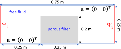
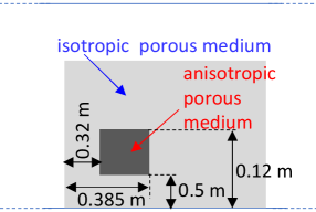
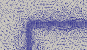
Figure 4: Test 2, settings of the numerical experiment. Homogeneous porous medium (left), heterogeneous porous medium (center), and zoom of the computational grid near the interface (right).

A channelized flow is established above the porous filter and the maximum value of the Reynolds number $Re$, computed according the to maximum flow velocity in the fluid region, the depth of the fluid channel above the obstacle, and the kinematic fluid viscosity, is $Re\in\left[0.2,0.22\right]$ and 2, 3 magnitude orders smaller in the porous block. Generally, in all the scenarios presented for this test case, the fluid flows primarily around the porous obstacle, being upward oriented before entering the obstacle and downward oriented after exiting it.

The computational grid $T_{h}$ has 161105 triangles and 80991 vertices, and the grid size ranges from $\simeq 2.25\cdot 10^{-03}$ m, in the bulk fluid and porous regions, to $\simeq 2.82\cdot 10^{-04}$ m, close to the interface. The time step size $\Delta t$ is 4 s. The ICs are zero velocity and pressure in the domain. In the following we show the results at the simulation time $\mathcal{T}=80$ s, when the steady state conditions are established.

In Section˜6.2.1 we consider homogeneous porous filter (see Fig.˜4, left) and different porous medium anisotropy conditions, while in Section˜6.2.2 we investigate how the method simulates a heterogeneous filter (see Fig.˜4, right) with strong contrast of porosity and permeability values.

6.2.1 Homogeneous porous medium

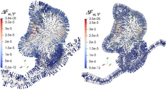
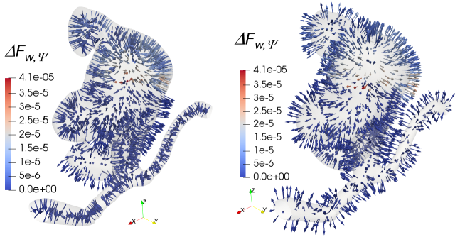
Figure 18: Test 4, computed difference in $\mathbf{F}_{w,\Psi}$ between the cases $F_{r}\simeq 1$ and $F_{r}\simeq 0.61$ (left) and between the cases $F_{r}\simeq 1$ and $F_{r}=0$ (right). Top row: $t=T_{0}/4$, bottom row: $t=3T_{0}/4$ (results in $\textnormal{m}^{4}/\textnormal{s}^{2}$).

The porosity in the porous filter is $\phi=0.4$, while the permeability $\mathbf{K}$ is computed as in (6.4). Fig.˜5 shows the velocity and pressure fields computed for method 1, setting $k=1\cdot 10^{-06}$ $\textnormal{m}^{2}$, $\beta=100$, and $\alpha=\pm\pi/4$. Due to the anisotropy effects in the porous filter, the flow, oriented according to the principal direction of the permeability tensor, exits or enters at the top horizontal side, if $\alpha=-\pi/4$ or $\alpha=\pi/4$, respectively. The pressure profiles are also aligned with the principal direction of the permeability tensor. The pressure exhibits very slight discontinuity across the top horizontal interface. In the case of $\alpha=-\pi/4$, the flow inside the filter is upward oriented. The opposite flow directions inside and outside the filter along the right interface create small vortices at the bottom of that interface. In the case of $\alpha=\pi/4$, the flow inside the filter is downward oriented. The opposite flow directions outside and intside the filter along the left interface create small vortices at the bottom of that interface. We obtained very similar results using smaller time step sizes $\Delta t$, not shown here for brevity. A very good agreement is observed with the results provided in [SCHNEIDER2020109012, , Fig. 5] and [Arico-ODA, , Fig. 18]. In SCHNEIDER2020109012 the authors apply a two-domain approach (TDA), coupling the Navier–Stokes equations (for compressible fluid) in the fluid region with the Darcy equation in the porous domain via the Beavers–Joseph–Saffman slip condition Beavers_Joseph_1967 , as well as conservation of mass and momentum, at the interface. They adopt a staggered-grid finite volume method for the Navier–Stokes equations and MPFA for Darcy flow, using uniform square grids grid with size $5\cdot 10^{-04}$ m. In Arico-ODA , a one-domain approach (ODA) with a transition layer is used to solve the Navier–Stokes–Brinkman equations for an incompressible fluid using a three-step predictor-corrector method. A finite volume method is applied for the predictor step, accounting for the inertial terms of the momentum equation, and two corrections are then performed to update the viscous and gradient pressure terms using a mass-lumped mixed hybrid finite element scheme with $RT_{0}$ basis functions. An unstructured triangular grid is used with mesh size ranging from $5\cdot 10^{-03}$ m in the bulk fluid and porous regions to $1\cdot 10^{-04}$ m in the transition layer. More details can be found in SCHNEIDER2020109012 , Arico-ODA .

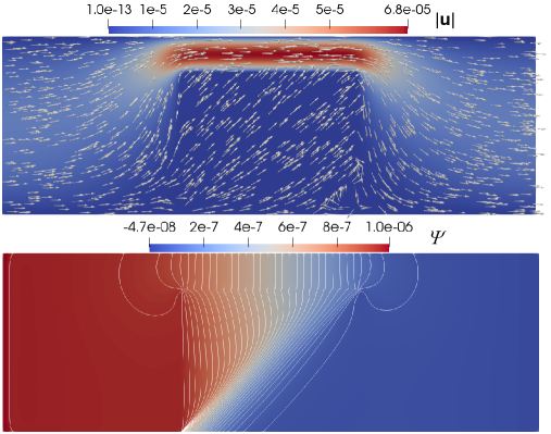
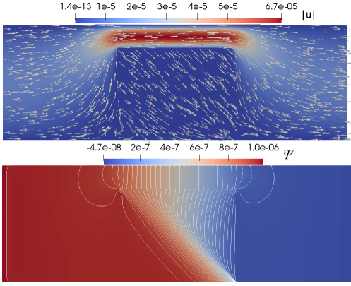
Figure 5: Test 2, homogeneous porous medium, $k=1\cdot 10^{-06}$, $\beta=100$. Computed velocity (top) and pressure (bottom) with method 1. Left: $\alpha=-\pi/4$, right: $\alpha=\pi/4$.

In Fig.˜6 we compare the velocity fields computed with method 1 (top) and method 2 (bottom). We observe irregular and non-physical vortical structures with method 2. We also ran a simulation using method 2 with $\Delta t=0.2$ s, obtaining results very similar to these on the top row of Fig.˜6 produced with method 1 and $\Delta t=4$ s. These results illustrate that, while method 2 is convergent, it may exhibit non-physical behavior for large time steps and requires smaller time steps than method 1 to produce an accurate solution. This is consistent with the fact that method 2 does not include the permeability correction term in the PjP and the pressure gradient update, cf. (4.15)–(4.16), which results in additional time-splitting error.

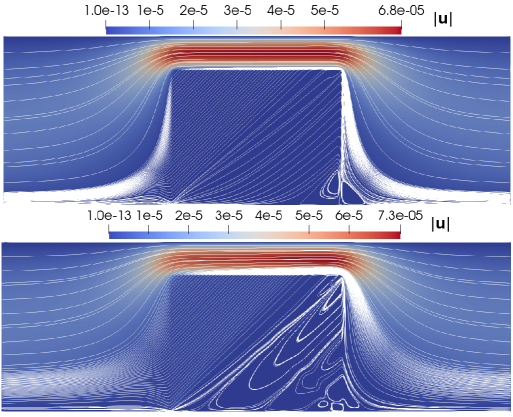
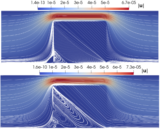
Figure 6: Test 2, homogeneous porous medium, $k=1\cdot 10^{-06}$, $\beta=100$. Computed velocity with method 1 (top) and method 2 (bottom). Left: $\alpha=-\pi/4$, right: $\alpha=\pi/4$.

In Fig.˜7 we show the results obtained by method 1 in the case of a strong vertical anisotropy, with $\alpha=0$, $k=1\cdot 10^{-06}$ $\textnormal{m}^{2}$ and $\beta=1000$, in which case the horizontal permeability is three orders of magnitude smaller than the vertical permeability. The fluid enters the filter primarily from the left side, mostly vertically upward oriented, concentrated in very thin stripe along the porous block boundary, see Fig.˜7 (top-left, top-right, and bottom-tight). This generates there a pressure gradient downward oriented, which explains the local minimum in the pressure field close to the left upper corner, see Fig.˜7 (bottom-left and top-right). Due to the high vertical permeability and the local pressure minimum, part of the channelized flow enters the porous medium from the top, downward oriented, close to the left upper corner, with velocity magnitude 2-3 magnitude orders smaller than in the region along to the left boundary, see Fig.˜7 (bottom-right). The opposite occurs close to the right boundary of the filter. A small amount of the flow exits at the top near the upper right corner, upward oriented, while most of the flow exits on the right side, downward oriented, concentrated in a thin stripe along the right boundary. The flow generates a strong pressure gradient upward oriented, which explains the local maximum in the pressure field close to the right upper corner. In the interior of the filter the flow is mostly horizontal, but its magnitude is much smaller compared to the flow along the vertical boundaries. The sharp change of the velocity field in the horizontal direction results in a pressure jump across the vertical boundaries, which is clearly evident in Fig.˜7 (top-right). This behavior is consistent with the balance of force interface condition in the two-domain Stokes–Darcy model. The pressure contour lines are vertically oriented and aligned with the anisotropy direction. We obtained very similar results using smaller time step sizes $\Delta t$, not shown here for brevity. This example illustrates the ability of the method to produce a physically accurate solution in a challenging setting with strong permeability anisotropy and complex flow behavior.

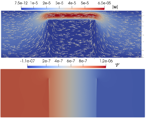
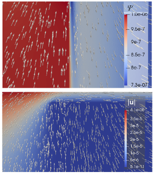
Figure 7: Test 2, homogeneous porous medium, $k=1\cdot 10^{-06}$, $\alpha=0$, $\beta=1000$. Computed velocity (top-left) and pressure (bottom-left) with method 1. Zooms of the velocity vectors and pressure field close to the left side of the filter (top-right) and close to the upper left corner of the filter (bottom-right).

In Fig.˜8 we compare the velocity fields in the case of the strong vertical anisotropy, ($k=1\cdot 10^{-06}$ $\textnormal{m}^{2}$, $\alpha=0$, $\beta=1000$), computed by method 1 (top, left) and method 2 (bottom, left), using $\Delta t$ = 2 s in method 2. While the general flow behavior is similar with both methods, we observe non-physical circular patterns in the velocity field computed with method 2. The zoom in of the pressure gradient and velocity vectors in Fig.˜8 (right) show that, while the pressure gradients in method 2 are aligned with the permeability anisotropy, the velocity vectors are not. We note that the solution obtained with method 2 using smaller time step of size $\Delta t=0.01$ s resembles the one obtained with method 1 using $\Delta t=4$ s.

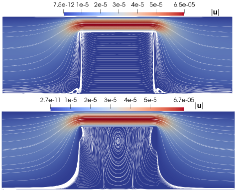
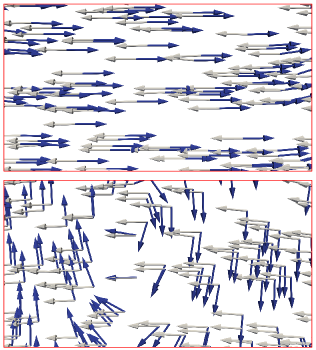
Figure 8: Test 2, homogeneous porous medium, $k=1\cdot 10^{-06}$, $\alpha=0$, $\beta=1000$. Left: computed velocity field with method 1 (top) and method 2 (bottom). Right: zoom in of the pressure gradient (gray) and velocity (blue) vectors computed with method 1 (top) and method 2 (bottom).

6.2.2 Heterogeneous porous medium

We investigate the capabilities of the proposed scheme to simulate flows in porous medium with strong contrast of the porosity and permeability tensor coefficients. We consider a porous filter composed by an outer isotropic region ($\phi=0.7$, $\alpha=0$, $\beta=1$, $k=1\cdot 10^{-06}$), with an inner anisotropic area $\Omega_{in}=\left(0.32,0.385\right)\times\left(0.5,0.12\right)$, see Fig.˜4 (right). In $\Omega_{in}$ we set $\phi=0.4$, $\alpha=\pi/4$, $\beta=100$ and $k=1\cdot 10^{-08}$ $\textnormal{m}^{2}$, resulting in a jump in the values of the porosity and permeability tensor coefficients across its boundary. In Fig.˜9 we show the velocity and pressure fields computed by method 1. The solver properly simulates the physical process: the velocity streamlines and the pressure contour lines deviate where the flow encounters the inner anisotropic region. We also compare in Fig.˜10 the velocity fields computed with method 1 (top) and method 2 (bottom). While method 2 produces a similar velocity field in the isotropic porous region, in the anisotropic region we observe some non-physical streamlines deviations and vorticities.

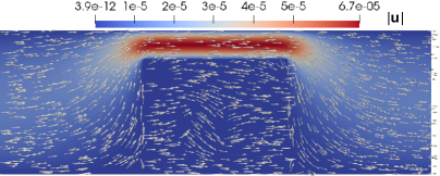
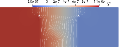
Figure 9: Test 2, heterogeneous porous medium. Computed velocity (left) and pressure (right) with method 1.

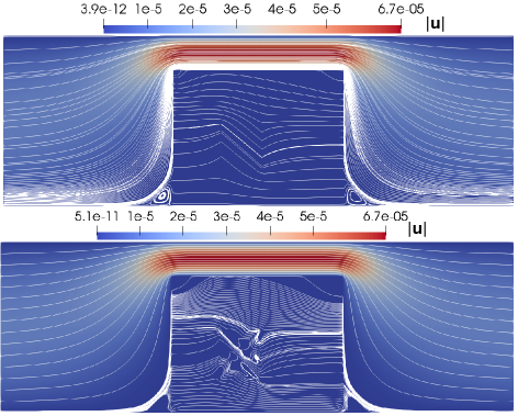
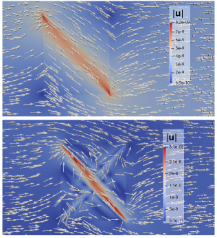
Figure 10: Test 2, heterogeneous porous medium. Velocity field computed with method 1 (top) and method 2 (bottom).

6.3 Test 3: interaction of a free fluid with a porous region with a steps-like interface

The setting of this test, presented in CHEN2014650 , is shown in Fig.˜11 (left). A polygonal interface with three steps divides the (dimensionless) computational domain $\Omega=(0,2)\times(0,2)$ in a fluid and a porous region. The Dirichlet boundary $\Gamma_{d}$ consists of the top and right sides of $\Omega$, with no-slip BCs on the top side and (dimensionless) Poiseuille velocity profile $\mathbf{u}=\left(\frac{y}{2}\left(y-2\right),0\right)^{T}$ on the right side. On the rest of the boundary we set $\bm{\Sigma}_{b}=0$. The ICs are zero velocity and pressure. The (dimensionless) kinematic viscosity is $\nu=1$. The medium is assumed to be isotropic with porosity and inverse permeability defined in (6.5). The porosity parameters are $\phi_{max}=1$ and $\phi_{min}=0.4$. Two (dimensionless) values of the inverse of the permeability coefficient are considered, $\mathfrak{K}^{0}_{i,i}=100$ and $\mathfrak{K}^{0}_{i,i}=10000$, $i=1,2$. According to CHEN2014650 , we set $\theta_{\psi}=\theta_{\mathfrak{K}_{i,j}}=100$ in the transition zone between the fluid and porous region. The Reynolds number in the fluid region, based on the maximum incoming velocity from the right side and the domain length side, is $Re=1$. In the porous region the maximum value of the Reynolds number is $Re\simeq 0.24$ if $\mathfrak{K}_{i,i}=100$ and $Re\simeq 0.0132$ if $\mathfrak{K}_{i,i}=10000$. We adopt a relatively coarse grid with (dimensionless) size ranging from 0.065 in the bulk fluid and porous regions to 0.02 in the transition region. The grid has 6421 triangles and 3281 vertices, see Fig.˜11 (right), similar to the one used in CHEN2014650 .

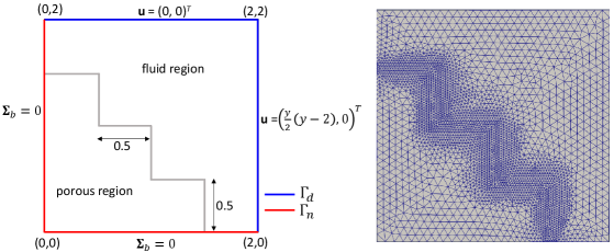
Figure 11: Test 3, settings of the numerical experiments (left) and computational grid (right).

In Figs.˜12 and 13 we plot the computed (dimensionless) velocity components and the (dimensionless) kinematic pressure fields with the velocity vectors. The flow enters the domain from the right vertical side. Due to the polygonal porous medium, the flow is partly channelized in the upper fluid region and partly leaves from the bottom side near the right corner, oriented downward. The velocity components are in very good agreement with the results in CHEN2014650 (see Figures 7 and 9 of the referred paper), where the authors solve the Brinkman equations in the framework of a ODA using Taylor–Hood finite elements. In the case of smaller permeability of the porous medium ($\mathfrak{K}_{i,i}=10000$), the flux leaving the domain downward oriented close to the right bottom step increases, see Fig.˜13 (center), which explains the local increment of the pressure seen in Fig.˜13 (right). We also observe higher deviations of the velocity vectors close to the interface with some vorticities. In Fig.˜14 we compare the profiles of $u_{x}$ at $x=0.5$ in the case of $\mathfrak{K}_{i,i}=10000$ computed by the present solver over the coarse grid (as detailed before), a much finer one (size ranging from 0.03 to 0.0075, with 30126 triangles and 15227 vertices) and the output obtained in CHEN2014650 (see Figure 11 in the referred paper). No evidence of any significant grid size effect is detected in the outputs of the present solver. The $u_{x}$ profile provided in CHEN2014650 is slightly shifted down, with a small underestimation of the peak value.

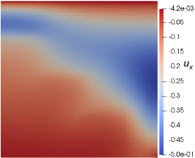
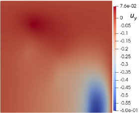
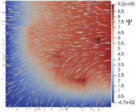
Figure 12: Test 3, computed $u_{x}$ (left), $u_{y}$ (middle), and $\Psi$ and velocity vectors (right) with $\mathfrak{K}_{i,i}=100$.

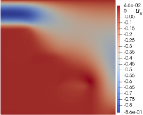
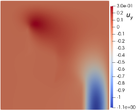
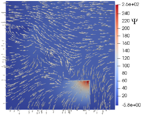
Figure 13: Test 3, computed $u_{x}$ (left), $u_{y}$ (middle), and $\Psi$ and velocity vectors (right) with $\mathfrak{K}_{i,i}=10000$.

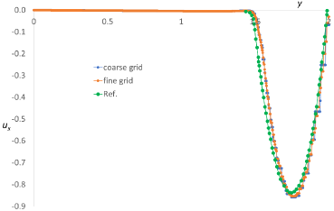
Figure 14: Test 3, profiles of $u_{x}$, $\mathfrak{K}_{i,i}=10000$. Nomenclature. “coarse grid” and “fine grid”: results of the present numerical method; “Ref.”: results provided in CHEN2014650 .

6.4 Test 4: Study of an intracranial aneurysm (ICA) with an aneurysmatic sac filled by a porous medium

The last test is a “show-case” application, where a porous medium fills the sac of an intracranial aneurysm (ICA). ICAs are dilatation of the arterial walls, generally formed in the circle of Willis, which may easily rupture, with consequent serious brain damages, hemorrhages, and high risk of mortality. During the last decade, a technology based on the use of porous media like shape memory polymer foams has been proposed as a novel endovascular ICA treatment, see, e.g., Cabaniss2025 and references therein. The shape memory property allows the polymers to be compressed into a catheter embedded into the ICA’s cavity, so that they expand via recovery activation, occupying the initial programmed ICA geometry, occluding the aneurysm cavity, and recovering the original cerebral parent vessel shape. This leads to a strong reduction of the blood circulation in the aneurysm cavity and stress on the internal walls of the sac. Clinical advantages have emerged over surgical treatments and the more traditional coiling techniques, the latter often involving a partial filling of the sac by the porous foam Cabaniss2025 .

We consider a real patient-specific geometry case-id “C0075” (patient-id “P0235”) of the open-source web repository “Aneurisk” AneuriskWeb , see the computational domain in Fig.˜15, left. The volume of the aneurysmatic sac is approximately 1180 $\textnormal{mm}^{3}$, one of the largest values in the web repository, and the diameter of the parent vessels is in the range $\left[1.7\cdot 10^{-03},3.4\cdot 10^{-03}\right]$ m. The computational grid has been created by the open-source VMTK toolkit Antiga2008 and Netgen Schberl1997NETGENAA , with 42915 vertices and 176102 tetrahedra with maximum aspect ratio 6.5. This application is presented to show the capability of the method to handle unsteady flows in very irregular domains.

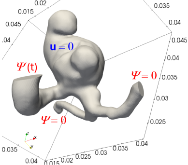
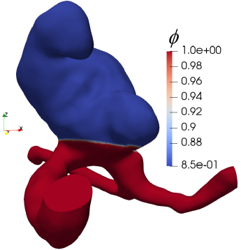
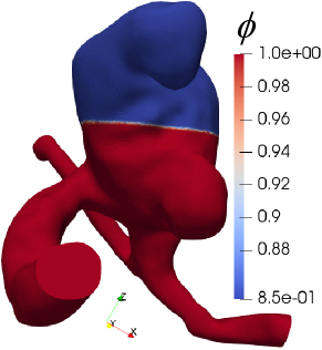
Figure 15: Test 4, computational domain and settings for the numerical runs (left), $\phi$ values for $F_{r}\simeq 1$ (center) and $\phi$ values for $F_{r}\simeq 0.61$ (right).

Table 22: Test 4, parameters of the porous medium within the aneurysmatic sac.

$\phi_{max}$	$\phi_{min}$	$\theta_{\psi}$	$\theta_{\mathfrak{K}_{i,j}}$	$\mathfrak{K}^{0}_{1,1}$	$\mathfrak{K}^{0}_{2,2}$	$\mathfrak{K}^{0}_{3,3}$	$\mathfrak{K}^{0}_{1,2}=\mathfrak{K}^{0}_{2,1}$	$\mathfrak{K}^{0}_{1,3}=\mathfrak{K}^{0}_{3,1}$	$\mathfrak{K}^{0}_{2,3}=\mathfrak{K}^{0}_{3,2}$
1	0.85	12000	12000	670	670	67000	0	0	0

We consider three scenarios, depending on the filling ratio of the aneurysmatic sac $F_{r}$, i.e., the ratio between the volume occupied by the porous medium and the total volume of the sac. The first two cases are shown in Fig.˜15 (center and right) corresponding to $F_{r}\simeq 1$ and $F_{r}\simeq 0.61$, respectively, while in the third scenario no porous medium fills the sac, i.e., $F_{r}=0$. The flow is generated by an unsteady periodic pressure difference $\Delta\Psi(t)=1\cdot 10^{-03}\sin(2\pi t)$ between the ends of the parent vessels, as shown in Fig.˜15 (left). We set zero velocity (no slip BCs) on the lateral vessel walls (Fig.˜15). The ICs are zero velocity and pressure. The porous medium in the sac is homogeneous and anisotropic. The porosity $\phi$ and the inverse permeability $\mathfrak{K}$ are computed as in (6.4) with parameters given in Table˜22. The permeability coefficient along the $z$ direction is two orders of magnitude smaller than along the other two directions.

We compute the hemodynamic forces on the internal wall of the ICA and on the porous medium filling the sac. The total forces on the ICA wall is computed as

$$\mathbf{F}_{w}=\mathbf{F}_{w,\Psi}+\mathbf{F}_{w,\nu}=\sum_{i=1}^{N_{fb}}\left(\mathbf{f}_{w,\Psi,i}+\mathbf{f}_{w,\nu,i}\right),$$

where the summation is over the triangles discretizing the ICA wall and $\mathbf{f}_{w,\Psi,i}$ and $\mathbf{f}_{w,\nu,i}$ are the pressure and viscous forces, respectively, acting on the $i$-th boundary triangle, $1\leq i\leq N_{fb}$, computed as

$$\mathbf{f}_{w,\Psi,i}=\phi_{i}\Psi_{i}\mathbf{n}_{i}|e_{i}|,\qquad f^{x\left(y,z\right)}_{w,\nu,i}=\nu\nabla u_{x\left(y,z\right)}^{n+1}\cdot\mathbf{n}_{i}|e_{i}|.$$

Here $|e_{i}|$ is the surface of interface $i$, $\phi_{i}$ is the porosity computed in the center of mass of the interface, $\Psi_{i}$ is the intrinsic kinematic pressure computed in the center of mass of $i$ according to the $P_{1}$ pressure distribution within the tetrahedron sharing the boundary interface, and $\mathbf{n}_{i}$ is the outward unit normal vector to the interface. $f^{x\left(y,z\right)}_{w,\nu,i}$ are the components of the viscous force $\mathbf{f}_{w,\nu,i}$, where the velocity components gradients are obtained according to the linear variation of the velocity components within the tetrahedron sharing the boundary face.

The force on the porous medium within the aneurysmatic sac is computed as

$$\mathbf{F}_{pm}=\sum_{i=1}^{N_{T,pm}}\mathbf{f}_{pm,i}=\sum_{i=1}^{N_{T,pm}}\sum_{j=1}^{d+1}\phi_{j}\mathbf{L}_{j}\mathbf{u}_{j}w_{j}|E_{i}|,$$

where the summation on $i$ is over the tetrahedra used to discretize the porous domain and $\mathbf{f}_{pm,i}$ is the force on the $i$-th element, computed by the Gaussian numerical integration. The summation on $j$ is over the $d+1$ Gaussian integration points within the $i$-th simplex with volume $|E_{i}|$, $\mathbf{L}_{j}$ and $\mathbf{u}_{j}$ are the quantities computed at the $j$-th integration point, and $w_{j}$ is the quadrature weight.

In Fig.˜16 we plot, for the case of $F_{r}\simeq 1$, the pressure and velocity fields at the simulation times $T_{0}/4$ and $3T_{0}/4$ (where $T_{0}$ is the oscillation period), corresponding to the maximum positive and negative pressure differences $\Delta\Psi$. The maximum Reynolds number in the vessel, computed according to the maximum velocity vector magnitude $|\mathbf{u}|$ and the diameter of the parent vessel, is $Re\simeq 0.3$. The maximum Reynolds number in the porous region is 2-3 orders of magnitude smaller. The velocity vectors are consistent with the pressure difference assigned at the boundary. Fig.˜17 shows the computed pressure and viscous forces acting on the ICA wall (left and middle columns) and the forces acting on the porous medium within the sac (right column). The magnitudes of $\mathbf{F}_{w,\nu}$ and $\mathbf{F}_{pm}$ are approximately 2 and 4 orders of magnitude smaller than the pressure forces $\mathbf{F}_{w,\Psi}$, respectively. As expected, $\mathbf{F}_{pm}$ is oriented according to the velocity within the porous medium, depending on the boundary assigned pressure differences. We further show in Fig.˜18 the differences in $\mathbf{F}_{w,\Psi}$ computed in the case $F_{r}\simeq 1$ with the cases $F_{r}\simeq 0.61$ and $F_{r}=0$. As expected, the magnitude of $\mathbf{F}_{w,\Psi}$ is smaller where the porous medium is in contact with the aneurysmatic wall.

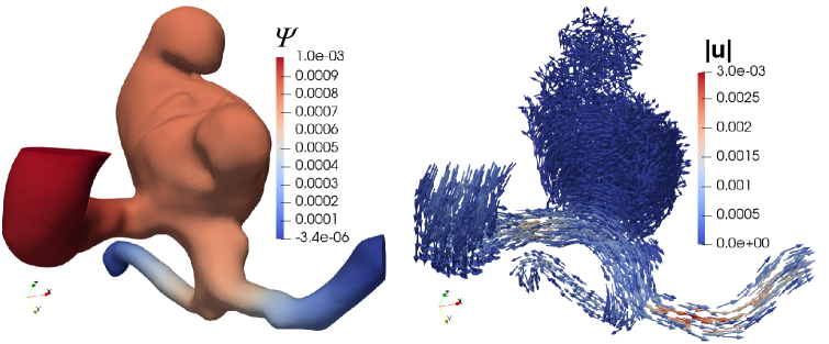
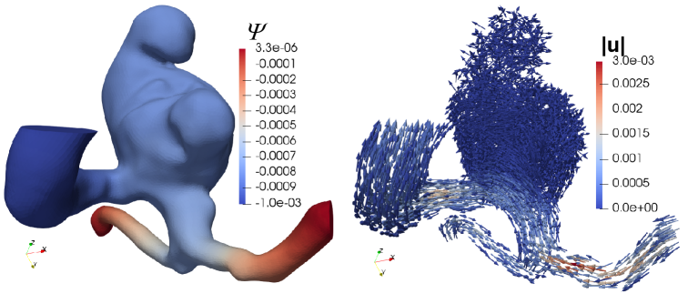
Figure 16: Test 4, computed results with $F_{r}\simeq 1$. Left: pressure ($\textnormal{m}^{2}/\textnormal{s}^{2}$), right: velocity ($\textnormal{m}/\textnormal{s}$). Top row: $t=T_{0}/4$, bottom row: $t=3T_{0}/4$.

.

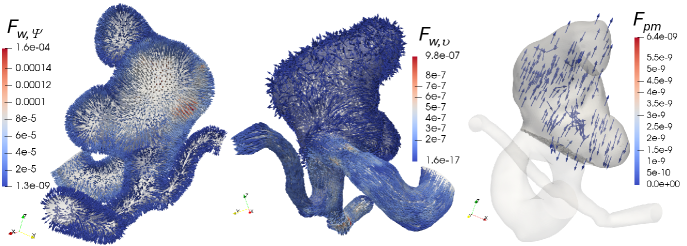
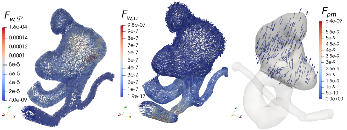
Figure 17: Test 4, computed results with $F_{r}\simeq 1$. Left: $\mathbf{F}_{w,\Psi}$, center: $\mathbf{F}_{w,\nu}$, right: $\mathbf{F}_{pm}$. Top row: $t=T_{0}/4$, bottom row: $t=3T_{0}/4$ (results in $\textnormal{m}^{4}/\textnormal{s}^{2}$).

7 Conclusions

We have presented $H(\text{div})$-conforming projection-based mixed finite element methods for the solution of the unsteady Brinkman problem. At each time step the methods require the solution of a mixed stress-velocity predictor problem for the viscous effects and a mixed velocity-pressure projection problem to account for the fluid incompressibility. The methods produce a pointwise divergence-free velocity and are robust in both the Stokes and the Darcy regimes. Unconditional stability of the fully discretized algorithm and first order in time accuracy have been established. In the second part of the paper, we proposed a specific method based on the MFMFE methodology on simplicial grids in 2D and 3D. We use the $RT_{1}$ mixed finite element pair along with an inexact numerical quadrature rule to obtain mass lumping and local elimination of the viscous stress and velocity in the prediction and projection problem, respectively. This results in symmetric and positive definite algebraic systems with only $d+1$ unknowns per element, efficiently solved by the preconditioned conjugate gradient method. The computed pressure and velocity are second order accurate in space. The numerical tests provided in this paper illustrate the efficiency and accuracy of the scheme for different benchmark problems, including challenging applications with highly irregular geometry and heterogeneous porous media with strong discontinuities of the porosity and permeability values. Furthermore, we show that the method is robust in both the Stokes and Darcy regimes and provides an efficient, accurate, and robust ODA alternative for modeling coupled free fluid and porous media flows.

References

- [1] J. Ahrens, B. Geveci, and C. Law. ParaView: An end-user tool for large data visualization. In Visualization Handbook. Elesvier, 2005.
- [2] V. Anaya, R. Caraballo, S. Caucao, L. F. Gatica, R. Ruiz-Baier, and I. Yotov. A vorticity-based mixed formulation for the unsteady Brinkman-Forchheimer equations. Comput. Methods Appl. Mech. Engrg., 404:Paper No. 115829, 30, 2023.
- [3] V. Anaya, G. N. Gatica, D. Mora, and R. Ruiz-Baier. An augmented velocity–vorticity–pressure formulation for the Brinkman equations. Int. J. Numer. Meth. Fl., 79(3):109–137, 2015.
- [4] Aneurisk-Team. AneuriskWeb project website, http://ecm2.mathcs.emory.edu/aneuriskweb. Web Site, 2012.
- [5] L. Antiga, M. Piccinelli, L. Botti, B. Ene-Iordache, A. Remuzzi, and D. A. Steinman. An image-based modeling framework for patient-specific computational hemodynamics. Med. & Biolog. Engrg & Comp., 46(11):1097–1112, Nov 2008.
- [6] T. Arbogast and D. S. Brunson. A computational method for approximating a Darcy-Stokes system governing a vuggy porous medium. Comput. Geosci., 11(3):207–218, 2007.
- [7] C. Aricò, R. Helmig, D. Puleo, and M. Schneider. A new numerical mesoscopic scale one-domain approach solver for free fluid/porous medium interaction. Comput. Methods Appl. Mech. Engrg., 419:Paper No. 116655, 28, 2024.
- [8] C. Aricò, M. Sinagra, C. Picone, and T. Tucciarelli. MAST-RT0 solution of the incompressible Navier-Stokes equations in 3D complex domains. Eng. Appl. Comput. Fluid Mech., 15(1):53–93, 2021.
- [9] C. Aricò, R. Helmig, and I. Yotov. Mixed finite element projection methods for the unsteady Stokes equations. Comput. Methods Appl. Mech. Engrg., 435:117616, 2025.
- [10] S. Badia and R. Codina. Unified stabilized finite element formulations for the Stokes and the Darcy problems. SIAM J. Numer. Anal., 47(3):1971–2000, 2009.
- [11] G. S. Beavers and D. D. Joseph. Boundary conditions at a naturally permeable wall. J. Fluid Mech., 30(1):197–207, 1967.
- [12] D. Boffi, F. Brezzi, and M. Fortin. Mixed finite element methods and applications, volume 44. Springer, 2013.
- [13] W. M. Boon, D. Gläser, R. Helmig, K. Weishaupt, and I. Yotov. A mortar method for the coupled Stokes-Darcy problem using the MAC scheme for Stokes and mixed finite elements for Darcy. Comput. Geosc., 28(3):413–430, Jun 2024.
- [14] H. C. Brinkman. A calculation of the viscous force exerted by a flowing fluid on a dense swarm of particles. Appl. Sci. Res., 1(1):27–34, 1949.
- [15] D. L. Brown, R. Cortez, and M. L. Minion. Accurate projection methods for the incompressible Navier-Stokes equations. J. Comput. Phys., 168(2):464–499, 2001.
- [16] E. Burman and P. Hansbo. Edge stabilization for the generalized Stokes problem: A continuous interior penalty method. Comput. Methods Appl. Mech. Engrg., 195(19):2393–2410, 2006.
- [17] E. Burman and P. Hansbo. A unified stabilized method for Stokes’ and Darcy’s equations. J. Comp. Appl. Math., 198(1):35–51, 2007.
- [18] R. Bustinza, G. N. Gatica, and M. González. A mixed finite element method for the generalized Stokes problem. Int. J. Num. Meth. Fluids, 49(8):877–903, 2005.
- [19] T. L. Cabaniss, R. Bodlak, Y. Liu, G. P. Colby, H. Lee, B. N. Bohnstedt, R. Garziera, G. A. Holzapfel, and C.-H. Lee. CFD investigations of a shape-memory polymer foam-based endovascular embolization device for the treatment of intracranial aneurysms. Biomech. Mod. Mechanobiology, 24(1):281–296, Feb 2025.
- [20] Z. Cai, C. Wang, and S. Zhang. Mixed finite element methods for incompressible flow: Stationary Navier–Stokes equations. SIAM J. Numer. Anal., 48(1):79–94, 2010.
- [21] J. Camaño, G. N. Gatica, R. Oyarzúa, R. Ruiz-Baier, and P. Venegas. New fully-mixed finite element methods for the Stokes–Darcy coupling. Comput. Methods Appl. Mech. Engrg., 295:362–395, 2015.
- [22] S. Caucao, T. Li, and I. Yotov. A multipoint stress-flux mixed finite element method for the Stokes-Biot model. Numer. Math., 152(2):411–473, 2022.
- [23] S. Caucao, R. Oyarzúa, S. Villa-Fuentes, and I. Yotov. A three-field Banach spaces-based mixed formulation for the unsteady Brinkman-Forchheimer equations. Comput. Methods Appl. Mech. Engrg., 394:Paper No. 114895, 32, 2022.
- [24] S. Caucao and I. Yotov. A Banach space mixed formulation for the unsteady Brinkman-Forchheimer equations. IMA J. Numer. Anal., 41(4):2708–2743, 2021.
- [25] M. Chandesris and D. Jamet. Boundary conditions at a planar fluid–porous interface for a Poiseuille flow. Int. J. Heat Mass Transf., 49(13):2137–2150, 2006.
- [26] H. Chen and X.-P. Wang. A one-domain approach for modeling and simulation of free fluid over a porous medium. J. Comp. Phys., 259:650–671, 2014.
- [27] M. Correa and A. Loula. A unified mixed formulation naturally coupling Stokes and Darcy flows. Comput. Methods Appl. Mech. Engrg., 198(33):2710–2722, 2009.
- [28] J. J. Dongarra., I. S. Duff., D. C. Sorensen, and H. V. D. Vorst. Solving Linear Systems on Vector and Shared Memory Computers. Society for Industrial and Applied Mathematics, 1990.
- [29] H. Egger and B. Radu. On a second-order multipoint flux mixed finite element methods on hybrid meshes. SIAM J. Num. Anal., 58(3):1822–1844, 2020.
- [30] G. N. Gatica, L. F. Gatica, and A. Márquez. Analysis of a pseudostress-based mixed finite element method for the Brinkman model of porous media flow. Numer. Math., 126(4):635–677, 2014.
- [31] G. N. Gatica, R. Oyarzúa, and F. J. Sayas. Analysis of fully-mixed finite element methods for the Stokes–Darcy coupled problem. Math. Comp., 80(276):1911–1948, 2011.
- [32] B. Goyeau, D. Lhuillier, D. Gobin, and M. Velarde. Momentum transport at a fluid–porous interface. Int. J. Heat Mass Trans., 46(21):4071–4081, 2003.
- [33] W. G. Gray. A derivation of the equations for multi-phase transport. Chem. Engi. Sc., 30(2):229–233, 1975.
- [34] J. Guermond, P. Minev, and J. Shen. An overview of projection methods for incompressible flows. Comput. Methods Appl. Mech. Engrg., 195(44):6011–6045, 2006.
- [35] J. Guzmán and M. Neilan. A family of nonconforming elements for the Brinkman problem. IMA J. Num. Anal., 32(4):1484–1508, 2012.
- [36] J. S. Howell, M. Neilan, and N. J. Walkington. A Dual–Mixed Finite Element Method for the Brinkman Problem. SMAI J. Comput. Math., 2:1–17, 2016.
- [37] O. Iliev and V. Laptev. On numerical simulation of flow through oil filters. Comp. Vis. Sc., 6(2):139–146, Mar 2004.
- [38] M. Juntunen and R. Stenberg. Analysis of finite element methods for the Brinkman problem. Calcolo, 47(3):129–147, 2010.
- [39] G. Kanschat and B. Rivière. A strongly conservative finite element method for the coupling of Stokes and Darcy flow. J. Comp. Phys., 229(17):5933–5943, 2010.
- [40] J. Könnö and R. Stenberg. -conforming finite elements for the Brinkman problem. Math. Models Methods Appl. Sci., 21(11):2227–2248, 2011.
- [41] J. Könnö and R. Stenberg. Numerical computations with -finite elements for the brinkman problem. Comput. Geosc., 16(1):139–158, Jan. 2012.
- [42] W. J. Layton, F. Schieweck, and I. Yotov. Coupling fluid flow with forous fedia flow. SIAM J. Num. Anal., 40(6):2195–2218, 2002.
- [43] M. Le Bars and M. G. Worster. Interfacial conditions between a pure fluid and a porous medium : implications for binary alloy solidification. J. Fluid Mech., 550:149–173, 2006.
- [44] K. Lipnikov, D. Vassilev, and I. Yotov. Discontinuous Galerkin and mimetic finite difference methods for coupled Stokes–Darcy flows on polygonal and polyhedral grids. Numer. Math., 126(2):321–360, Feb 2014.
- [45] K. A. Mardal, X.-C. Tai, and R. Winther. A Robust Finite Element Method for Darcy–Stokes flow. SIAM J. Num. Anal., 40(5):1605–1631, 2002.
- [46] A. Masud. A stabilized mixed finite element method for Darcy-Stokes flow. Intern. J. Numer. Meth. Fl., 54(6-8):665–681, 2007.
- [47] L. Mu. A Uniformly Robust H(DIV) weak Galerkin Finite Element Methods for Brinkman Problems. SIAM J. Num. Anal., 58(3):1422–1439, 2020.
- [48] L. Mu, J. Wang, and X. Ye. A stable numerical algorithm for the Brinkman equations by weak Galerkin finite element methods. J. Comp. Phys., 273:327–342, 2014.
- [49] K. Nafa and A. J. Wathen. Local projection stabilized Galerkin approximations for the generalized Stokes problem. Comput. Methods Appl. Mech. Engrg., 198(5):877–883, 2009.
- [50] J. Ochoa-Tapia and S. Whitaker. Momentum transfer at the boundary between a porous medium and a homogeneous fluid—i. theoretical development. Int. J. Heat Mass Transf., 38(14):2635–2646, 1995.
- [51] Y. Qian, S. Wu, and F. Wang. A mixed discontinuous Galerkin method with symmetric stress for Brinkman problem based on the velocity–pseudostress formulation. Comput. Methods Appl. Mech. Engrg., 368:113177, 2020.
- [52] A. Quarteroni and A. Valli. Numerical approximation of partial differential equations, volume 23 of Springer Series in Computational Mathematics. Springer-Verlag, Berlin, 1994.
- [53] P. A. Raviart and J. M. Thomas. A mixed finite element method for 2-nd order elliptic problems. In I. Galligani and E. Magenes, editors, Mathematical Aspects of Finite Element Methods, pages 292–315, Berlin, Heidelberg, 1977. Springer Berlin Heidelberg.
- [54] B. Rivière and I. Yotov. Locally conservative coupling of Stokes and Darcy flows. SIAM J. Num. Anal., 42(5):1959–1977, 2005.
- [55] M. Schneider, K. Weishaupt, D. Gläser, W. M. Boon, and R. Helmig. Coupling staggered-grid and MPFA finite volume methods for free flow/porous-medium flow problems. J. Comp. Phys., 401:109012, 2020.
- [56] J. Schöberl. NETGEN an advancing front 2D/3D-mesh generator based on abstract rules. Comput. Vis. Sci., 1:41–52, 1997.
- [57] D. Vassilev and I. Yotov. Coupling Stokes–Darcy flow with transport. SIAM J. Sci. Comp., 31(5):3661–3684, 2009.
- [58] P. S. Vassilevski and U. Villa. A Mixed Formulation for the Brinkman problem. SIAM J. Num. Anal., 52(1):258–281, 2014.
- [59] M. F. Wheeler and I. Yotov. A Multipoint Flux Mixed Finite Element Method. SIAM J. Numer. Anal., 44(5):2082–2106, 2006.
- [60] S. Whitaker. Flow in porous media I: A theoretical derivation of Darcy’s law. Transport Porous Med., 1, 1986.
- [61] X. Xie, J. Xu, and J. Xue. Uniformly Stable Finite Element Methods for Darcy-Stokes-Brinkman Models. J. Comput. Math., 26(3):437–455, 2008.
- [62] L. Zhao, E. Chung, and M. F. Lam. A new staggered DG method for the Brinkman problem robust in the Darcy and Stokes limits. Comput. Methods Appl. Mech. Engrg., 364:112986, 2020.