Non-universal Thermal Hall Responses in Fractional Quantum Hall Droplets

Abstract

We analytically compute the thermal Hall conductance (THC) of fractional quantum Hall droplets under realistic conditions that go beyond the idealized linear edge theory with conformal symmetry. Specifically, we consider finite-size effects at low temperature, nonzero self-energies of quasiholes, and general edge dispersions. We derive measurable corrections in THC that align well with the experimental observables. Although the quantized THC is commonly regarded as a topological invariant that is independent of edge confinement, our results show that this quantization remains robust only for arbitrary edge dispersion in the thermodynamic limit. Furthermore, the THC contributed by Abelian modes can become extremely sensitive to finite-size effects and irregular confining potentials in any realistic experimental system. In contrast, non-Abelian modes show robust THC signatures under perturbations, indicating an intrinsic stability of non-Abelian anyons.

Introduction. The fractional quantum Hall (FQH) effect is one of the most astonishing phenomena in condensed matter physics. It emerges in a two-dimensional ($2$D) electron system subjected to a strong magnetic field and extremely low temperature, where the Hall resistance is quantized at specific rational values [1, 2]. The robustness of the fractional Hall plateau cannot be explained by either single-particle quantum mechanics or classical solid-state physics, since it is essentially a strong-coupling quantum many-body problem induced by a quenched kinetic energy and a broken time-reversal symmetry [3, 4, 5]. Furthermore, the quasiparticles in FQH fluids were confirmed to carry fractional charges and obey anyonic statistics [6, 7, 8, 9]. In particular, quasiparticles in non-Abelian FQH phases are believed to be a promising platform for fault-tolerant quantum computation [10, 11, 12, 13]. The lattice analogy of such quantum fluids, known as the fractional Chern insulators, has also been realized in twisted bilayer systems and pentalayer graphene [14, 15, 16]. In quantum Hall (QH) fluids, there exist measurable quantities that cannot change smoothly, which encode the symmetry and naturally the topology [17, 18, 6, 5, 19, 20, 21]. Extracting topological indices from transport experiments typically requires focusing on the edge of the FQH fluid, since the bulk behaves as an insulator while the edge hosts gapless excitations that encode the same topological information[4, 22, 23]. Besides the well-known quantized Hall plateau in charge transport, the thermal Hall conductance (THC) is predicted as a topological quantity since it is universal assuming a linear dispersion at the edge in the thermodynamic limit [24]. Several recent experiments have shown that the quantized value of the THC could be used to distinguish different candidate phases, especially at the half-filling [25, 26, 27, 28, 29].

The edges of QH phases are effectively described by chiral Luttinger liquids [30, 31]. The THC from chiral edge modes is proportional to the central charge $c$ of the underlying $(1+1)$D conformal field theory (CFT) that characterizes the edge [32, 24, 33, 34, 35, 36]. The universality of the THC thus depends on conformal symmetry, typically requiring a linear dispersion in the edge modes. However, under realistic experimental conditions, additional factors can contribute to deviations in the measured THC, such as insufficient thermal equilibration due to finite-size effects, quasihole self-energy corrections induced by non-ideal interactions, and nontrivial edge dispersions arising from irregular confining potentials. Considerations of realistic conditions bring non-universal correction terms to the universal quantized value. These effects are especially relevant for understanding why thermal Hall measurements have so far shown significantly lower precision than their electric counterparts, and the recently observed THC value at half filling with a controversial origin [25, 26, 27, 28, 29, 37, 38, 39].

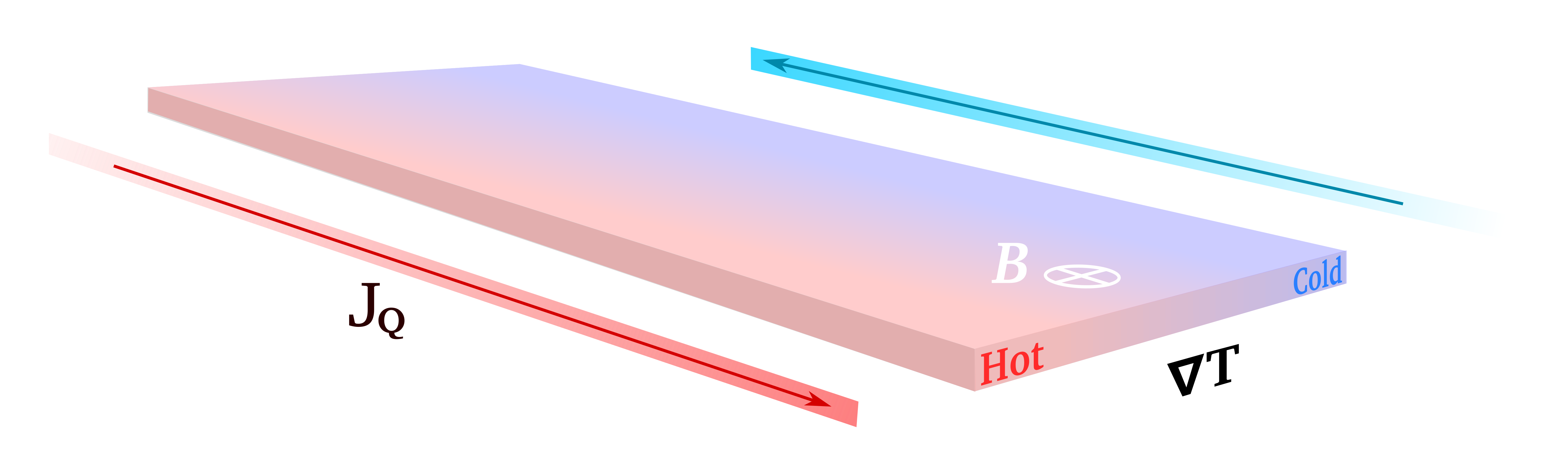
Figure 1: Schematic diagram of the thermal Hall effect in a fractional quantum Hall (FQH) system. Under a large magnetic field $B$, the two-dimensional electron gas forms an FQH phase in the bulk of the sample, characterized by chiral, gapless edge states. When a temperature gradient $\nabla T$ is applied, these edge states carry a heat current $J_{Q}$ (indicated by red and blue arrows) that flows perpendicular to $\nabla T$. The resulting thermal Hall conductance serves as a topological invariant of the bulk FQH phase.

In this letter, we provide a systematic analysis of corrections to the thermal Hall conductance $\kappa$ in FQH states under various conditions, including finite-size effects, nonzero quasihole self-energies, and general edge dispersions. Rather than relying on mesoscopic transport modeling such as the Landauer-Buttiker formalism, we microscopically construct the edge partition function and build up thermodynamic quantities determining $\kappa$ for both Abelian and non-Abelian phases, where ground-state wave functions are Jack polynomials [40, 41]. We then use numerical calculations to confirm the predicted behavior of $\kappa$ under these conditions. Our results show that the THC for the non-Abelian edge modes remains stable against both finite-size effects and nonzero quasihole self-energies in a canonical ensemble describing an FQH droplet. In contrast, Abelian modes exhibit significant corrections to $\kappa$ under the same perturbations. We also find that the THC is no longer a universal quantity in realistic systems if the edge dispersion is not strictly linear. In particular, the usual relation between specific heat, THC, and central charge breaks down in the nonlinear regime. The techniques used in this work can be readily extended to other systems with quantized THC, such as other FQH states and the spin liquid. The non-universal corrections we derive accurately account for the deviations in existing THC measurements [42, 25, 43, 29]. These corrections may also be used to distinguish between different asymptotic behaviors of the candidate states at the same filling. For example, the well-known non-Abelian candidate states for $\nu=5/2$, which can be Pfaffian ($c=7/2$), anti-Pfaffian ($c=3/2$), or the PH-Pfaffian ($c=5/2$), can be predicted by using the non-universal correction terms of THC.

Thermal Hall conductance on a disk. Consider a Hall bar with a longitudinal temperature gradient between its top and bottom edges. In response, a transverse thermal current will emerge (see Fig. 1). This phenomenon, known as the Leduc-Righi effect, is the thermal analog of the Hall effect [44, 45, 46]. The THC is defined as:

$$\kappa=\frac{\partial J_{Q}}{\partial T},$$ (1)

where $J_{Q}$ is the thermal current and $T$ is the temperature at the edge. It has been predicted in Ref.[24] that the THC at the edge of an FQH system is quantized, proportional to the central charge $c$ of the CFT that effectively describes the edge physics:

$$\kappa=\kappa_{0}\cdot T\cdot c,$$ (2)

where $\kappa_{0}=\pi^{2}k_{B}^{2}/(3h)$, $k_{B}$ is the Boltzmann constant and $h$ is the Planck constant. However, the THC is proportional to $c$ only under certain ideal situations. For FQH states with Abelian edge modes, each of them will contribute one unit of THC ($c=1$). In contrast, when the FQH state hosts non-Abelian edge modes, $c$ can take fractional values [33]. For example, a Majorana edge mode contributes a central charge of $c=1/2$ [47, 5]. If multiple edge modes propagate in the same direction, their contributions to $c$ or the THC are additive; If the edge modes propagate in opposite directions, the net THC is given by the difference between the downstream and upstream contributions [33]. In either case, thermal equilibration between edge modes is essential to ensure ballistic thermal transport. [24].

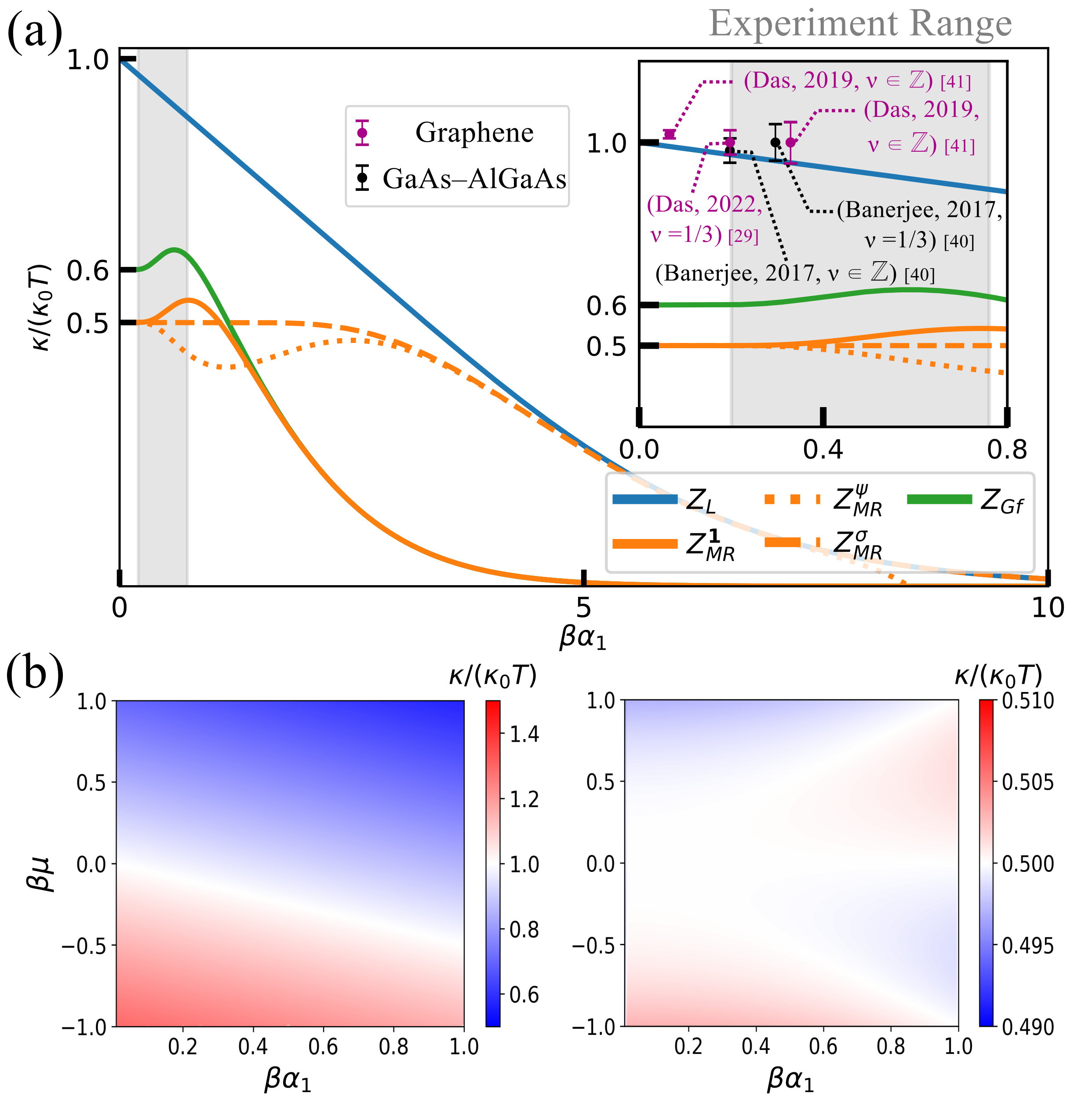
Figure 2: Non-universal thermal Hall responses of different edge modes.(a) Thermal Hall conductance (THC) of Abelian, non-Abelian Majorana, and the non-Abelian (NA) component of Gaffnian edge modes as a function of $\beta\alpha_{1}$. At $\beta\alpha_{1}=0$, the value of $\kappa/(\kappa_{0}T)$ matches the central charge. For the Abelian $U(1)$ mode (blue curve), the THC decreases almost linearly once $\beta\alpha_{1}$ is turned on. In contrast, the Majorana modes (orange curves, with different line types denoting distinct topological sectors) and the NA component of the Gaffnian mode (green curve) remain nearly constant over a wide range of $\beta\alpha_{1}$, indicating the robustness of non-Abelian modes against finite-size effects. The inset zooms in on the experimentally relevant regime (gray area) and displays available measurement data for the $U(1)$ sector in various systems, aligning well with theoretical predictions. (b) The THC of the Abelian $U(1)$ mode (left panel) decreases linearly with tuning parameters such as quasihole creation energy and edge mode velocity, while the THC of the Majorana fermion mode (right panel) remains essentially unaffected, further demonstrating its insensitivity to microscopic details.

Let $\Delta k$ be the minimal linear momentum of quasihole states relative to the ground state, and $v_{F}$ the Fermi velocity of the corresponding edge mode, which is treated as a constant for all modes (although different modes can have different velocities). If the system is in the thermodynamic regime (i.e., a high-temperature limit relative to level spacing), we have:

$$k_{B}T\gg\hbar v_{F}\Delta k.$$ (3)

This condition ensures that the THC remains quantized and thus topological. Since $\Delta k$ depends on the system size, there is a competition between two experimental parameters, temperature $T$ and system size $L$. To capture this interplay, we define a dimensionless parameter $\beta\alpha_{1}$ with $\alpha_{1}=hv_{F}/L$ (the subscript $1$ denotes a linear dispersion) and $\beta=1/(k_{B}T)$ to study the THC in other different regimes.

To understand edge excitations microscopically, we consider an FQH fluid on a disk with circumference $L$ and $N$ electrons. Due to rotational invariance, angular momentum $m$ serves as a good quantum number for classifying states. When a magnetic flux is adiabatically inserted into the bulk, electrons will get pushed towards the edge by a radial current, effectively creating a quasihole in the bulk [3]. Each quasihole formed in the bulk induces a density modulation at the edge, giving rise to a specific edge mode. As a result, edge excitations can be classified according to the angular momentum of the corresponding quasihole states: We define the ground state angular momentum as $m_{0}$ and denote $p(\Delta m)$ as the degeneracy of quasihole states in the angular momentum sector $m$ with $\Delta m=m-m_{0}$. In the thermodynamic limit, the edge channels can be treated as one-dimensional with the linear momentum $k=m/L$. This is a working example of the bulk-edge correspondence [48, 49, 50].

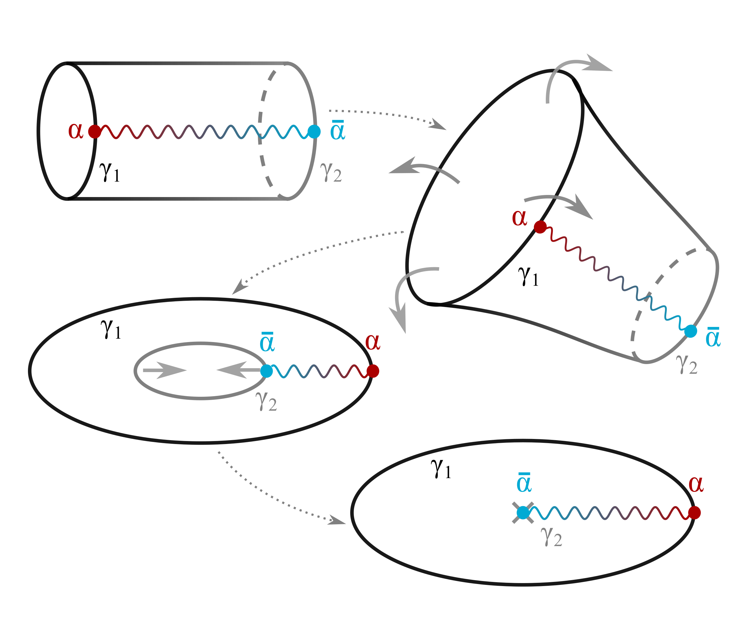
Figure 3: Mapping from cylinder to disk geometry. On a cylinder with two chiral edges $\gamma_{1,2}$, inserting a flux through the hole is equivalent to nucleating a conjugate anyon pair $(a,\bar{a})$ in the bulk, and one can drag them to opposite boundaries, represented by an open Wilson line stretching between $\gamma_{1}$ and $\gamma_{2}$. Here, the bulk-edge correspondence appears as a gluing condition that originates from electron locality and enforces conjugate anyon charges on the two edges. Shrinking $\gamma_{2}$ to a point in the bulk maps the cylinder to a disk, where the Wilson line now terminates at the single boundary $\gamma_{1}$. In this limit, the cylinder gluing condition gives the bulk-edge correspondence on the disk, i.e., the bulk fixes the topological sector of the remaining edge, thereby determining the Majorana boundary condition (NS or R), the parity, and the $U(1)_{2}$ charge sector of the Moore-Read edge CFT. The resulting disk partition functions are the corresponding character combinations [51].

We can hence write down the partition function describing the FQH edge as:

$$Z=\sum_{\Delta m=0}^{\infty}\>\sum_{\xi=1}^{p(\Delta m)}\>e^{-\beta\epsilon_{m,\xi}}.$$ (4)

Here, the $\xi$ is the index of the quasihole states in the same $m$ sector, and $\epsilon_{m,\xi}$ denotes the energy of the quasihole state. Applying a parabolic confining electrostatic potential at the edge leads to edge excitations with a linear dispersion relation $\epsilon_{m,\xi}=v_{F}\>\Delta m$, where $v_{F}$ is the effective Fermi velocity of chiral edge modes [52]. States in the same $m$ sector can correspond to different numbers of quasiholes, determined by the insertion of different numbers of magnetic fluxes. In principle, all thermodynamic observables of the edge system can be systematically derived from $Z$.

Finite-size corrections of THC. The temperature in FQH experiments is not highly tunable, as it must remain sufficiently low to stabilize the FQH phase. Therefore, in the following analysis, we refer to the corrections associated with a nonzero $\alpha_{1}$ as finite-size effects. Physically, this means that the system size/temperature is not large/high enough for the system to reach the thermodynamic limit.

We begin by focusing on the chiral $U(1)$ bosonic edge modes common to all Laughlin states, including the integer QH phases. As a concrete example, we consider the $\nu=1/3$ Laughlin state with linear dispersion and vanishing quasihole self-energies. The degeneracy (or density of states) at each angular momentum sector $p(\Delta m)$ for quasihole excitations in any Laughlin state with the filling $\nu=1/(2k+1),k\in\mathbb{Z}_{+}$ is the same, given by the Virasoro counting identical to the integer partition number of $\Delta m$ (i.e., the number of ways for positive integers to add up to $\Delta m$.) [49], $1,1,2,3,5,7,\cdots$, which gives a partition function of Abelian edge excitations with particle number $N\rightarrow\infty$:

$$Z_{L}^{(\infty)}=\sum_{\Delta m=0}^{\infty}p(\Delta m)e^{-\beta\alpha_{1}\Delta m}=\frac{1}{(q)_{\infty}},$$ (5)

where $q\equiv e^{-\beta\alpha_{1}}$, $(q)_{n}\equiv\prod_{i=1}^{n}(1-q^{i})$ and $(q)_{\infty}\equiv\text{lim}_{n\rightarrow\infty}(q)_{n}$, and we omitted the contribution from the ground state $\propto q^{N^{2}/2}$ [34]. Mathematically, Eq. 5 is the generating function for unrestricted integer partitions [53]. We can then obtain the specific heat of the Laughlin edge in the asymptotic limit of $\beta\alpha_{1}\rightarrow 0$ as :

$$C_{L}= \sum_{j=1}^{\infty}(j\beta\alpha_{1})^{2}\frac{e^{-j\beta\alpha_{1}}}{(1-e^{-j\beta\alpha_{1}})^{2}}\sim\frac{\pi^{2}}{3\beta\alpha_{1}}-\frac{1}{2}+\mathcal{O}(\beta,\alpha_{1}).$$ (6)

Here $\sim$ denotes “asymptotically equivalent to”. Finally, the THC of the Laughlin edge modes under linear dispersion in the asymptotic limit is:

$$\kappa_{L}= \frac{v_{F}}{L}C_{L}=\kappa_{0}T\left(1-\frac{3}{2\pi^{2}}\beta\alpha_{1}+\mathcal{O}(\beta^{2},\alpha_{1}^{2})\right)$$ (7)

This gives the central charge of the Laughlin states as $c=1$ in the limit of $\beta\alpha_{1}\rightarrow 0$.

Assuming the Fermi velocity of the chiral boson edge state to be in the range of $5\times 10^{6}$ cm/s $\sim 1.5\times 10^{7}$ cm/s for the 2-dimensional electron gas (2DEG) in GaAs, as estimated from numerical analysis [55], the $\beta\alpha_{1}$ in the actual experiment is about $0.20$ to $0.76$, corresponding to a correction of around $0.03$ to $0.12$ to the value of specific heat and thus the THC at $10$ mK. In transport experiments, one can expect a more accurate estimate of $\kappa$ for greater finite-size effects using a grand canonical ensemble [33]. The experimental error range has been reported, e.g., in Ref. [42] for the Laughlin phase at $\nu=1/3$, where the measured THC was $\kappa=(1.0\pm 0.045)\ \kappa_{0}T$. Notably, the uncertainty is on the order of $\mathcal{O}(10^{-2})$, which is significantly larger than the precision typically achieved in Hall conductance measurements.

We now study the thermal Hall responses in non-Abelian phases using the half-filling Moore-Read (MR) phase. In this case, two types of modes contribute to the edge excitations, the Abelian chiral boson modes and the non-Abelian Majorana fermion modes [5, 56]. The former corresponds to the Abelian $U(1)_{2}$ sector, while Majorana fermions are described by the Ising CFT with primary fields $\{\mathbf{1},\psi,\sigma\}$ [57]. In the thermodynamic limit, the MR quasihole states obey the generalized Pauli principle that there can only be at most two particles in four consecutive angular momentum orbitals, as the defining property from the model Hamiltonian [40]. The counting in the first few angular momentum sectors of MR quasiholes $p_{p}(\Delta m)$ is $1,1,3,5,10,16,\cdots$, leading to a partition function with particle number $N\rightarrow\infty$ to be [34, 53]:

$$Z_{\text{MR}}^{(\infty)}=\frac{1}{(q)_{\infty}}\sum_{n=0}^{\infty}\frac{q^{\frac{n^{2}}{2}}}{(q)_{n}}=\frac{1}{(q)_{\infty}}\prod_{j=0}^{\infty}\left(1+q^{j+1/2}\right).$$ (8)

The factor $1/{(q)_{\infty}}$ in Eq. 8 represents the Abelian $U(1)_{2}$ charge sector (as in Eq. 5), while the remaining piece encodes the neutral Majorana fermion modes. Note that Eq. 8 sums over the two partition functions (i.e., the Neveu-Schwarz (NS) characters) [56]:

$$Z_{\text{MR}}^{\mathbf{1}} =\frac{1}{2(q)_{\infty}}\left[\prod_{j=0}^{\infty}\left(1+q^{j+1/2}\right)+\prod_{j=0}^{\infty}\left(1-q^{j+1/2}\right)\right],$$ (9)

$$Z_{\text{MR}}^{\mathbf{\psi}} =\frac{1}{2(q)_{\infty}}\left[\prod_{j=0}^{\infty}\left(1+q^{j+1/2}\right)-\prod_{j=0}^{\infty}\left(1-q^{j+1/2}\right)\right],$$

and thus does not resolve parity subsectors. In a finite droplet, however, such a distinction is essential since locality of the electron operator requires a gluing condition between the Majorana and $U(1)_{2}$ sectors [58, 56, 51]. Microscopically, this means that the parity of the electron number and the distribution of bulk anyons fix the Majorana sector. Hence on a disk, even $N$ selects $Z_{\text{MR}}^{\mathbf{1}}$, while odd $N$ selects $Z_{\text{MR}}^{\mathbf{\psi}}$ .

In contrast to the NS sectors, the Ramond (R) sector does not contribute to the edge partition function unless bulk $-e/4$ quasiholes are present, as the fusion rules $\psi\times\sigma=\sigma$ and $\sigma\times\sigma=1+\psi$ suggest. One way to visualize this is by the Wilson-line picture on a cylinder, where the line connecting an anyon pair enforces the parity constraint, equivalent to the bulk-edge correspondence upon mapping to a disk, as shown in Fig. 3. The corresponding disk partition function in the $R$ sector takes the form:

$$Z_{\text{MR}}^{\sigma}=\frac{1}{(q)_{\infty}}\prod_{j=1}^{\infty}\left(1+q^{j}\right).$$ (10)

The presence or absence of these bulk quasiholes gives rise to the well-known odd-even effect of the Moore-Read state as a direct signature of non-Abelian statistics, i.e., the interference pattern in a $\nu=5/2$ Fabry-Pérot interferometer is predicted to depend on whether the number of bulk $-e/4$ quasiholes is even or odd, with the odd case suppressing interference [59, 60].

In the thermodynamic limit, one can prove that both the sector- and parity-resolved of MR partition functions and their average flow to the same chiral central charge $c=3/2$ and thus converge to the same quantized THC . We obtain the specific heat contributed by the Majorana fermions in the asymptotic limit $(\beta\alpha_{1}\rightarrow 0)$ to be:

$$C_{MF}\sim\frac{\pi^{2}}{3\beta\alpha_{1}}\frac{1}{2}+\mathcal{O}(\beta^{2},\alpha_{1}^{2})$$ (11)

Interestingly, we find that the leading-order correction term (linear in $\beta\alpha_{1}$) for the Majorana fermion modes vanishes regardless of the parity or the boundary condition, indicating the intrinsic robustness of the non-Abelian modes. As illustrated in Fig. 2a, finite-size systems exhibit the same robustness of $\kappa$ across all sectors near $\beta\alpha_{1}=0$. However, for larger deviations, the corrections become both parity- and sector-dependent. Hence, besides interference measurements, parity-resolved deviations in $\kappa$ offer another potential experimental benchmark for non-Abelian topological order. Finally, the leading order THC of the MR edge contributed by both $U(1)_{2}$ bosons and Majorana fermions under linear dispersion is:

$$\kappa_{MR}=\kappa_{0}T\left(\frac{3}{2}-\frac{3}{2\pi^{2}}\beta\alpha_{1}+\mathcal{O}(\beta^{2},\alpha_{1}^{2})\right).$$ (12)

This shows the total central charge of the MR state as $c=1+1/2=3/2$, with the finite-size corrections mainly contributed by the Abelian mode.

Non-zero self-energy of quasiholes. Quasiholes and thus edge modes are conventionally treated as a non-interacting “ideal gas”, which serves as a good approximation in the dilute limit. Tuning on the interactions between edge modes generally renormalizes the Fermi velocity $v_{F}$ without significantly affecting THC [24, 55]. Additionally, quasiholes are assumed to be “massless”, meaning their creation does not require finite energy upon flux insertion. However, this condition is generally not true with realistic interactions between electrons, as confirmed by extensive numerical calculations [61, 62]. To capture such effects, we write the partition function as:

$$Z_{qh} =\sum_{\Delta m=0}^{\infty}\tilde{p}(\beta,\Delta m)\cdot e^{-\beta\alpha_{1}\Delta m},$$ (13)

where the effective density of state at a finite temperature $\tilde{p}(\beta,\Delta m)$ reads:

$$\tilde{p}(\beta,\Delta m) =\sum_{\xi=1}^{p(\Delta m)}e^{-\beta\tilde{\epsilon}_{m,\xi}}.$$ (14)

Here $\tilde{\epsilon}_{m,\xi}$ depends on the details of the quasihole states labeled by $\xi$ within the angular momentum $m$ sector, which generically contains a different number of interacting quasiholes. Since increasing temperature eventually destroys FQH phases, the original density of states $p(\Delta m)$ will reappear only when the quasihole self-energy is small compared to the thermal energy. This also implies that conformal invariance is effectively restored at the zero self-energy limit.

We now reconsider the Laughlin phase. When a quasihole is created in the FQH droplet, the total energy of the quantum fluid decreases due to the repulsive interactions among electrons. As a result, quasiholes acquire a negative self-energy (or “mass”). Assuming that each flux insertion carries a constant energy cost $\mu$, and that the quasiholes form a dilute, non-interacting gas, we can write down the modified partition function of the Laughlin edge modes as:

$$Z_{L,qh} =\sum_{\Delta m=0}^{\infty}\sum_{\xi=1}^{p(\Delta m)}e^{-\beta\alpha_{1}\Delta m}e^{-\beta\tilde{\epsilon}_{m,\xi}}=\prod_{i=1}^{\infty}\frac{1}{1-tq^{i}},$$ (15)

where $t\equiv e^{-\beta\mu}$, and $\tilde{\epsilon}_{m,\xi}=\epsilon_{m,\xi}-\alpha_{1}\Delta m$ is the total quasihole self-energy of the excitation state $\xi$, i.e, the product of $\mu$ and the number of quasiholes in state $\xi$. If we further assume the velocity of the edge mode remains the same as in the ideal case, the asymptotic THC is now:

$$\kappa_{L,qh}=\kappa_{0}T\bigg(1-\frac{3}{2\pi^{2}}\beta(\alpha_{1}+2\mu)+\mathcal{O}(\beta^{2},\alpha_{1}^{2},\mu^{2})\bigg)$$ (16)

which agrees well with numerical calculations in Fig. 2b. The additional correction enhances the THC when the quasihole creation energy $\mu$ is negative, since it increases the effective density of states at finite temperatures.

Similarly, we can obtain the modified THC of the MR phase. Assuming that all types of quasiholes contributing to both chiral boson mode and Majorana fermion mode have the self-energy $\mu$, the partition function of the Majorana fermion mode is given by:

$$Z_{MF,qh}=\prod_{n=0}^{\infty}(1+q^{n+\frac{1}{2}}t^{\frac{1}{2}}),$$ (17)

while the resultant THC turns out to be invariant:

$$\kappa_{MF,qh}=\kappa_{0}T\left(\frac{1}{2}+\mathcal{O}(\beta^{2},\alpha_{1}^{2},\mu^{2})\right).$$ (18)

in the sense that the THC does not linearly dependent on $\beta\alpha_{1}$ and $\beta\mu$.

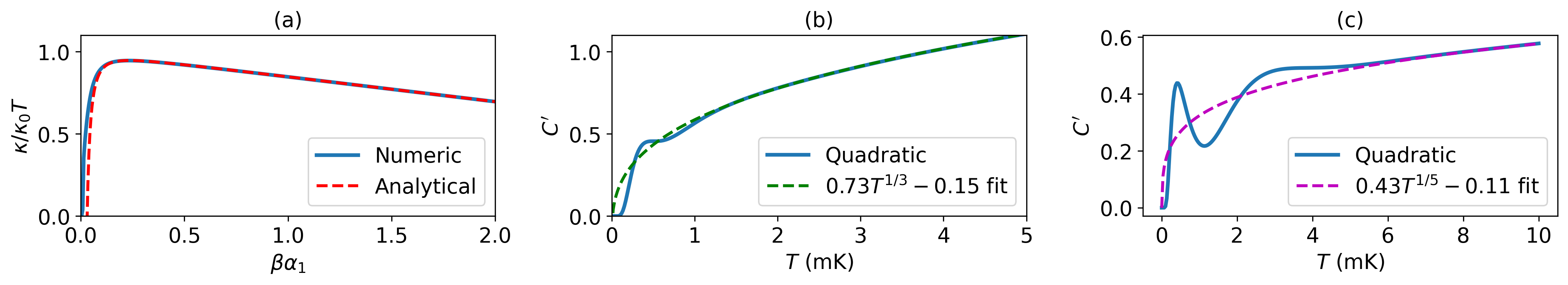
Figure 4: Thermodynamic observables under nonlinear dispersions. (a) The THC of Abelian modes under a more general dispersion $\epsilon_{m}=\alpha_{1}\Delta m+\alpha_{2}(\Delta m)^{2}$ where $\alpha_{2}$ is chosen to be $10^{-4}$ such that $\alpha_{2}\ll\alpha_{1}$. The dashed line represents the analytical solution that are presented in Eq. 20 in the limit of $\beta\alpha_{1}\rightarrow 0$. (b) and (c) show the normalized specific heat $C^{\prime}=\frac{k_{B}}{\alpha_{n}^{2}}C_{L}$ versus temperature $T$ under different dispersions. Both $\alpha_{2}$ and $\alpha_{3}$ are estimated to be in the order of $10^{-26}$. The dashed line represents the fitting curve under the high-temperature limit. Under quadratic/cubic dispersion, $C_{L}$ is proportional to $\sqrt[3]{T}$/$\sqrt[5]{T}$.

To briefly summarize the preceding discussions, there is an intrinsic instability of THC components from Abelian modes. Meanwhile, for the Majorana mode, the quantized THC remains stable under finite-temperature effects, even in the presence of a non-vanishing quasihole self-energy. This suggests an intrinsic robustness rooted in the non-Abelian nature of its anyonic statistics. We further confirmed this by calculating the THC for the Gaffnian state with non-Abelian modes, as shown in Fig. 2a, which shows a similar robustness.

Generic THC with nonlinear dispersion. In the thermodynamic limit, our microscopic approach with discrete angular momentum $m$ becomes equivalent to the Luttinger liquid formalism with continuous momentum $k$ [63, 64, 31, 24, 65]. Taking the chiral $U(1)$ boson modes as an example, we can establish the correspondence by invoking $f_{B}(\epsilon_{k})=(e^{\beta\epsilon_{k}}-1)^{-1}$ with an arbitrary dispersion relation $\epsilon_{k}$ and derive the THC as:

$$\kappa_{U(1)}=\frac{1}{2\pi}\int_{0}^{\infty}\>dk\>\frac{\partial\epsilon_{k}}{\partial k}\>\frac{(\beta\epsilon_{k})^{2}\>e^{\beta\epsilon_{k}}}{(e^{\beta\epsilon_{k}}-1)^{2}}=\frac{\pi^{2}k_{B}^{2}}{3h}T.$$ (19)

which is irrelevant to $\epsilon_{k}$ and thus universal. However, when finite-size effects are taken into account, such universality vanishes, which can be seen from the Euler-Maclaurin formula . Moreover, the commonly assumed linear dispersion of edge modes relies on the idealization that the confining potential at the sample boundary is perfectly quadratic. In realistic QH systems, the edge potential is generally not strictly quadratic, and deviations from this assumption can lead to significant nonlinearities in the edge-mode dispersion. It is therefore instructive to analyze simplified models that go beyond the linear-dispersion approximation, where the conformal symmetry of the edge theory is explicitly broken.

We first consider the case where the energy dispersion is not perfectly linear $\epsilon_{m}=\alpha_{1}\Delta m+\alpha_{2}(\Delta m)^{2}$, where $\alpha_{2}\ll\alpha_{1}$ is the quadratic dispersion coefficient. By taking the Laughlin state at $\nu=1/3$ and assuming that the degeneracy of each $\Delta m$ sector is not affected, we can obtain the asymptotic THC ($\beta\alpha_{1}\rightarrow 0$) as:

$$\kappa_{L}\approx\kappa_{0}T\left(1-\frac{3}{2\pi^{2}}\beta\alpha_{1}-\pi^{2}\frac{\alpha_{2}}{\alpha_{1}^{3}\beta^{2}}\right)$$ (20)

where the extra correction term is due to the quadratic component of the dispersion relation . This is further confirmed by numerical results as shown in Fig.4(a), in which the THC is reduced and the quantity $\kappa/(\kappa_{0}T)$ at the limit of $\beta\alpha_{1}\rightarrow 0$ is no longer representing the central charge.

Next, we show that the specific heat will be decoupled from the THC if the energy dispersion is purely nonlinear. We take the power-law dispersion $\epsilon_{m}=\alpha_{n}(\Delta m)^{n}$, where $\alpha_{n}$ is the dispersion coefficient, the modified partition function for the $\nu=1/3$ Laughlin state is given by:

$$Z_{L,ND}=\sum_{\Delta m=0}^{\infty}p(\Delta m)e^{-\beta\alpha_{n}(\Delta m)^{n}}$$ (21)

Under the limit $\beta\alpha_{n}\rightarrow 0$, such a partition function gives the relationship between the specific heat and the temperature as :

$$C_{L}\propto T^{\frac{1}{2n-1}}$$ (22)

This is further confirmed by numerical results as shown in Fig. 4, where the coefficients in Eq. 22 fit well. However, when the dispersion relation becomes nonlinear, the THC ceases to scale linearly with the heat capacity, since the propagation velocity of the edge modes varies across different angular momentum sectors $m$. To analyze this effect, let us consider a generic FQH edge state with a known degeneracy structure for each $m$ sector. The thermal current can then be written as:

$$J_{Q}=\sum_{\Delta m=0}^{\infty}v_{m}\frac{\epsilon_{m}}{L}\frac{p(\Delta m)e^{-\beta\epsilon_{m}}}{Z}$$ (23)

where $\epsilon_{m}$ is the energy of the mode, $v_{m}$ is the velocity of the modes and $Z$ is the partition function.

We can express the THC in a more general form :

$$\kappa=-\frac{\beta^{2}}{2\pi\hbar}\frac{\partial}{\partial\beta}\bigg[\frac{1}{Z}\frac{\partial}{\partial\beta}\bigg(\frac{1}{\beta}\frac{\partial Z}{\partial(\Delta m)}\bigg)\bigg]$$ (24)

Eq. 24 gives us the relationship between the edge partition function and the THC independent of the dispersion relation. In the special case of a linear dispersion, the heat capacity is given by $C=\beta^{2}\cdot\partial^{2}_{\beta}log(Z)$, leading to the conventional relation $\kappa=\frac{v_{F}}{L}C$. Therefore, the THC is the product of the edge-mode velocity and the specific heat only with a linear dispersion. When nonlinear effects are present, one must instead use Eq. 23. This clarifies why Eq. 19 in the effective model holds only when the edge theory is approximated by a strictly linear dispersion.

We now employ Eq. 24 to investigate the impact of a quadratic dispersion, $\epsilon_{m}=\alpha_{2}(\Delta m)^{2}$, on the THC of the Laughlin edge mode, under the assumption that the degeneracy $p(\Delta m)$ remains unchanged. In this case, the THC can be expressed as

$$\frac{\kappa}{\kappa_{0}T}=\frac{6}{\pi^{2}}\,\gamma^{3}\bigg(\frac{1}{Z}Z_{5}-\frac{1}{Z^{2}}\,Z_{2}\,Z_{3}\bigg),$$ (25)

where $\gamma=\beta\alpha_{2}$ and the generalized generating function is defined as

$$Z_{n}=\sum_{\Delta m=0}^{\infty}p(\Delta m)\,(\Delta m)^{n}\,e^{-\gamma(\Delta m)^{2}}.$$ (26)

More generally, for a power-law dispersion of the form $\epsilon_{m}=\alpha_{n}(\Delta m)^{n}$, the THC can be generalized to

$$\frac{\kappa}{\kappa_{0}T}=\frac{3n}{\pi^{2}}\,\gamma^{3}\bigg(\frac{1}{Z}Z_{3n-1}-\frac{1}{Z^{2}}\,Z_{n}\,Z_{2n-1}\bigg),$$ (27)

provided that the degeneracy $p(\Delta m)$ remains invariant under changes in the order of the dispersion relation.

Summary and Discussions. In conclusion, we have studied the nonuniversal behaviours in the THC of both the Laughlin and Moore-Read states under different effects. We find that the THC contribution from non-Abelian edge modes remains robust under finite-size corrections, suggesting an intrinsic stability of Majorana excitations whose microscopic origin requires further study. In contrast, the THC of the $U(1)$ chiral boson mode decreases linearly with $\beta\alpha_{1}$, providing an estimate for errors observed in THC experiments under certain valid assumptions. Accounting for a finite quasihole creation energy preserves the quantization of the non-Abelian contribution, while the $U(1)$ bosonic sector remains susceptible to perturbations. When nonlinear dispersion effects arising from realistic confinement potentials are included, the standard proportionality between THC, specific heat, and chiral central charge breaks down. For the Laughlin state, assuming the same degeneracy pattern $p(\Delta m)=(1,1,2,3,5,7,\dots)$ as in the linear case leads to a loss of THC universality and a nontrivial relation to heat capacity. We therefore conclude that THC retains its universal quantization for any dispersion in the thermodynamic limit, but in finite-size systems, nonlinear dispersions can significantly alter its value.

Recent thermal transport experiments have reported a THC value of $\kappa=2.5$, which has been interpreted as evidence for a particle-hole (PH) Pfaffian phase, despite this phase not being favored in finite-size numerical studies [25, 28]. Accurately describing these experiments requires accounting for interaction-induced edge reconstructions, long-wavelength disorders, differences in edge mode velocities, and thermal equilibration processes. It has been proposed that the observed THC may result from a Majorana edge mode remaining out of thermal equilibrium [37]. However, a complete understanding of the experimental results also necessitates considering momentum mismatches between counterpropagating modes. Recent studies also suggest that edge reconstructions in the Majorana sector can lead to an effective PH Pfaffian signature [66]. Further experimental proposals will be the key to confirming and reconciling the mechanism behind the measured THC values.

Our results provide additional experimentally accessible parameters from a different perspective that can help distinguish the contributions of different edge modes. Although different statistical ensembles become equivalent in the thermodynamic limit, notable discrepancies can arise when this limit is not reached. Transport experiments are generally best described within a grand canonical ensemble, but we propose an alternative approach using quantum Hall droplet calorimetry, which naturally realizes a canonical ensemble. Such droplets can, in principle, be engineered by electrostatic confinement or gate-defined potentials that isolate mesoscopic regions of the 2DEG [67]. To access the specific heat of edge modes and the THC, one can inject a controlled amount of power locally into the edge channels (for example via noise or bias at a point contact) and monitor the resulting temperature rise at a nearby sensor. Recent local-power protocols have demonstrated how to directly quantify the power carried by edge modes and extract $\kappa$ without relying on conventional two-terminal transport measurements, even in the absence of full thermal equilibration between counter-propagating branches [68, 69]. Looking forward, moiré platforms hosting FCIs (e.g., twisted MoTe₂) offer particularly promising testbeds. Their micron-scale flakes combine low electronic heat capacity, sharp edges, and van der Waals stacking that naturally accommodates contactless heaters and noise-based thermometry, raising the possibility of probing $\kappa$ in a canonical setting. We leave a systematic investigation of measuring $\kappa$ in FCI systems for future work.

Supplementary material of “Non-universal Behaviors of Thermal Hall Conductance in Fractional Quantum Hall States”

In the supplementary material, we provide detailed technical analyses that support and extend the results in the main text. To help readers quickly locate topics of interest, we provide a summary of the content for each section below. In Sec. A, we develop the Mellin transform method in analytic number theory to study the asymptotic behavior of logarithmic generating functions and thus the finite-size and nonzero-self-energy corrections to the thermal Hall conductance (THC), with detailed discussions for Laughlin phases (chiral boson modes), different sectors in the Majorana fermion phase, and the non-Abelian modes in the Gaffnian phase. In Sec. B, we show that the THC ceases to be universal under the combined action of finite-size effects and a general dispersion relation. In Sec. C, we specialize to the Laughlin $\nu=1/3$ state and examine its THC under the quadratic correction to the dispersion relation ($\epsilon=\alpha_{1}n+\alpha_{2}n^{2}$). In Sec. D, we provide exact derivations of the heat capacity to leading order for arbitrary power-law dispersions of Laughlin edge modes, where $\epsilon_{m}=\alpha_{k}(\Delta m)^{k}$. Finally, in Sec. E, we establish the general relation between the THC (or thermal current) and the partition function $Z$, independent of the underlying dispersion.

Appendix A Asymptotic behavior of thermal Hall conductance

In this section, we introduce a powerful technique in analytic number theory called the Mellin transform, which can help solve the asymptotic behavior of logarithmic generating functions near the singularity at $0$ or $\infty$ with series-product identities, where it is normally hard to solve the Laurent series directly. In our case, we are interested in knowing the expression of THC when $q\rightarrow 0$ (or $\beta\alpha_{1}\rightarrow 0$). However, the THC is not well-defined at this point since it will diverge so one has to study the asymptotic behavior of the functions (see 32).

A.1 Mellin transform

For $x\in\mathbb{R}_{+}$, the Mellin transform of a function $f(x)$is defined as:

$$f^{\star}(s)=\int_{0}^{\infty}f(x)\cdot x^{s-1}dx,\quad s\in\mathbb{C}.$$ (28)

Here $s$ should be constrained to a strip, i.e. $a<\text{Re}(s)<b$ where $f^{*}$ exists. The inverse transform can be written as:

$$f(x)=\frac{1}{2\pi i}\int_{c-i\infty}^{c+i\infty}f^{\star}(s)\cdot x^{-s}ds,$$ (29)

and we denote the Mellin dual as:

$$f(x)=\mathcal{M}^{-1}[f^{\star}(s)],\quad f^{\star}(s)=\mathcal{M}[f(x)].$$ (30)

This transform has the harmonic sum property:

$$\sum_{j}\lambda_{j}f\left(\omega_{j}\cdot x\right)\stackrel{{\scriptstyle\mathcal{M}}}{{\mapsto}}\left(\sum_{j}\lambda_{j}\cdot\omega_{j}^{-s}\right)\cdot f^{\star}(s),$$ (31)

which implies that one can factorize the harmonic sum of $f(x)$ to the product of a generalized Dirichlet series and $f^{*}(s)$. Essentially, the asymptotic expansion of different orders at $0$ or $\infty$ is described by the residues at different poles. This is extremely powerful when dealing with generating functions, considering they are essentially formal infinite function series.

Some properties of Mellin transforms and the Mellin dual functions that we will use in this paper are presented in Table. A.1:

Function	Mellin Transform	Fundamental Strip
$f(x)$	$f^{\star}(s)=\int_{0}^{\infty}f(x)x^{s-1}dx$	$a<\text{Re}(s)<b$
$x^{\nu}f(x)$	$f^{\star}(s+\nu)$	$a-\text{Re}(\nu)<\text{Re}(s)<b-\text{Re}(\nu)$
$f^{\prime}(x)$	$-(s-1)\cdot f^{\star}(s-1)$	$a+1<\text{Re}(s)<b+1$
$x^{\nu}f(x)$	$f^{\star}(s+\nu)$	$a+1<\text{Re}(s)<b+1$
$e^{-px},p>0$	$p^{-s}\cdot\Gamma(s)$	$0<\text{Re}(s)<\infty$
$(e^{ax}-1)^{-1},Re(a)>0$	$a^{-s}\cdot\Gamma(s)\cdot\zeta(s)$	$1<\text{Re}(s)<\infty$
$(e^{ax}+1)^{-1},Re(a)>0$	$a^{-s}\cdot\Gamma(s)\cdot\zeta(s)\cdot(1-2^{1-s})$	$0<\text{Re}(s)<\infty$
$(e^{-ax})(1-e^{-x})^{-1},Re(a)>0$	$\Gamma(s)\cdot\zeta(s,a)$	$1<\text{Re}(s)<\infty$

Table A.1: Some special function and their Mellin transformed functions. The third column shows the constraint of $s$ at the strip [70].

A.2 Chiral bosonic edge mode

The chiral bosonic (e.g., the edge modes in the Laughlin states) edge heat capacity reads:

$$C_{U(1)}= \sum_{j=1}^{\infty}(j\gamma)^{2}\frac{e^{-j\gamma}}{(1-e^{-j\gamma})^{2}},$$ (32)

where $\gamma=\beta\alpha_{1}$. Here, the ”amplitude” $\lambda_{j}=1$, the ”frequency” $\omega_{j}=j$ and the function $f(x)=x^{2}\frac{e^{-x}}{(1-e^{-x})^{2}}$. This can thus transform into:

$$\left(\sum_{j}j^{-s}\right)\cdot f^{\star}(s)=\zeta(s)\cdot\zeta(s+1)\cdot\Gamma(s+2),$$ (33)

where we have used the properties of the Mellin transform:

$$f^{\prime}(x)\stackrel{{\scriptstyle\mathcal{M}}}{{\mapsto}} -(s-1)\cdot f^{\star}(s-1)$$ (34)

$$x^{\nu}f(x)\stackrel{{\scriptstyle\mathcal{M}}}{{\mapsto}} f^{\star}(s+\nu),$$

and considered the following properties:

$$\Gamma(s+1)= \int_{0}^{\infty}t^{s}e^{-t}dt=\left.t^{s}\left(-e^{-t}\right)\right|_{0}^{\infty}-\int_{0}^{\infty}\left(-e^{-t}\right)st^{s-1}dt=s\int_{0}^{\infty}t^{s-1}e^{-t}dt=s\cdot\Gamma(s).$$ (35)

Here, $\zeta(s)$ is the Riemann zeta function (which has a pole when the argument is $1$) and $\Gamma(s)$ is the Gamma function (which has a pole when the argument is $0$ or negative integers). Therefore, Eq. 33 contains poles at $s=1,0,-2,-3...$ (see Fig. A.1). However, we only need to consider the poles at $s=0,1$, since the Riemann zeta function is zero for negative even integers. By using the residue theorem, we can thus obtain the heat capacity in the asymptotic limit, which gives the same result as the first approach and thus shows the flexibility of the Mellin transform:

$$C_{U(1)} =\sum_{n=-1}^{1}\ \text{Res}[\zeta(s)\ \zeta(s+1)\Gamma(s+2)\cdot x^{-s},n]$$ (36)

$$=\zeta(-1)\ \zeta(0)\ \Gamma(1)\cdot x+\zeta(0)\cdot\text{Res}[\zeta(s+1),s=0]\cdot\Gamma(2)+\text{Res}[\zeta(s),s=1]\cdot\zeta(2)\ \Gamma(3)\cdot x^{-1}$$

$$=\frac{x}{24}-\frac{1}{2}+\frac{\pi^{2}}{3x}\sim\frac{\pi^{2}}{3x}\bigg(1-\frac{3}{2\pi^{2}}x\bigg)+\mathcal{O}(x),$$

where we only keep the lowest-ordered correction term.

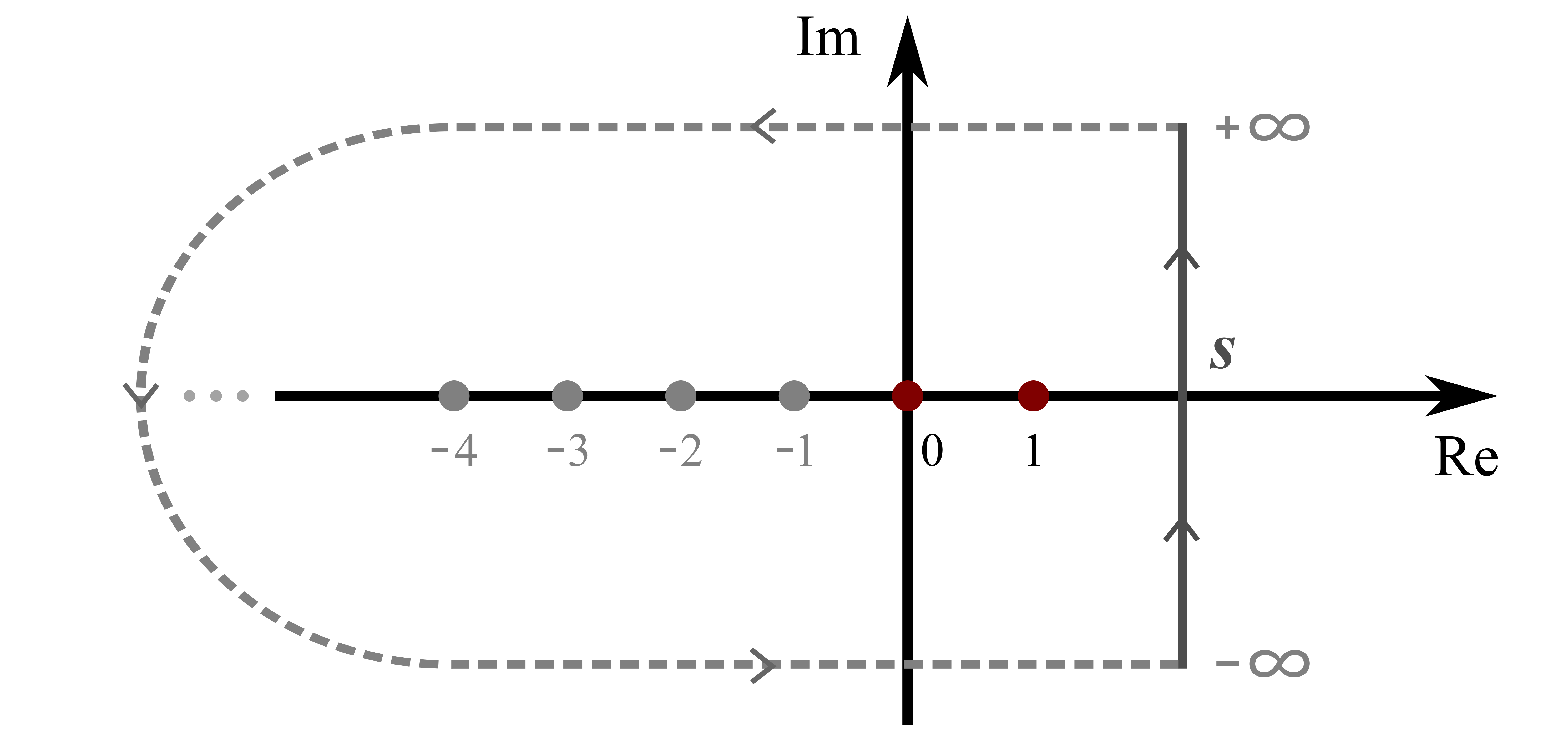
Figure A.1: Contour plot with poles for the U(1) modes specific heat. The $\zeta(s)$ contributes the pole at $s=1$, $\zeta(s+1)$ contributes pole at $s=0$, and $\Gamma(s+2)$ contribute poles at $s=-2,-3,-4...$

A.3 Majorana fermionic edge mode

	Thin Torus		Bulk TQFT/Edge CFT			Disk
Boundary	Occupations	Wave functions	Primary Fields	Parity	Characters $(r=1,2)$	$N\in\mathbb{N}$	$N\rightarrow\infty$
NS sector	11001100 $\cdots$	$\operatorname{Pf}\left(\frac{\vartheta_{a}\left(z_{i}-z_{j}\right)}{\vartheta_{1}\left(z_{i}-z_{j}\right)}\right)\Psi_{1/2}^{(t)}$, $a\in\{3,4\}$	$e^{i\phi/\sqrt{2}}$	P=1	$\chi_{0}^{\text{Ising }}\cdot\left(\chi_{r/2}^{+}+\chi_{r/2}^{-}\right)$	$Z_{MR}^{\mathbf{1}}$	$Z_{\text{MR}}^{(\infty)}$
	00110011 $\cdots$		$e^{-i\phi/\sqrt{2}}$		$\chi_{1/2}^{\text{Ising }}\cdot\left(\chi_{r/2}^{+}-\chi_{r/2}^{-}\right)$
	10011001 $\cdots$		$\psi\cdot e^{i\phi/\sqrt{2}}$	P=-1	$\chi_{1/2}^{\text{Ising }}\cdot\left(\chi_{r/2}^{+}+\chi_{r/2}^{-}\right)$	$Z_{MR}^{\psi}$
	01100110 $\cdots$		$\psi\cdot e^{-i\phi/\sqrt{2}}$		$\chi_{0}^{\text{Ising }}\cdot\left(\chi_{r/2}^{+}-\chi_{r/2}^{-}\right)$
R sector	10101010 $\cdots$	$\operatorname{Pf}\left(\frac{\vartheta_{2}\left(z_{i}-z_{j}\right)}{\vartheta_{1}\left(z_{i}-z_{j}\right)}\right)\Psi_{1/2}^{(t)}$	$\sigma\cdot e^{i\phi/(2\sqrt{2})}$ $\sigma\cdot e^{-i\phi/(2\sqrt{2})}$	–	$\chi_{1/16}^{\text{Ising }}\cdot\chi_{(r+1/2)/2}^{+}$	$Z_{MR}^{\sigma}$
	01010101 $\cdots$

Table A.2: Correspondence between thin-torus occupation patterns, conformal field theory (CFT) descriptions of the Moore-Read (MR) Pfaffian edge, and disk partition functions. In the thin-torus (Tao-Thouless) limit, the six topologically distinct MR ground states appear as crystalline occupation patterns such as $1100\,1100\cdots$ or $1010\,1010\cdots$, where the quasihole and quasiparticle excitations can be interpreted as domain walls between these different patterns (or “vacua”) [71, 72]. Their real-space wave functions are Pfaffians of Jacobi theta functions $\vartheta_{a}(z)$ multiplied by the bosonic Laughlin state at $\nu=1/2$ on torus, $\Psi_{1/2}^{(t)}=\prod_{i<j}\vartheta_{1}\left(\left.\frac{z_{i}-z_{j}}{L_{1}}\right\rvert\,i\frac{L_{2}}{L_{1}}\right)^{2}$, where $L_{1},L_{2}$ are the periods of torus, and the Pfaffian factor encodes pairing correlations [56, 73]. In the edge CFT description, the MR state factorizes into a neutral Majorana fermion (Ising CFT with primary fields $\mathbf{1}$, $\psi$, and $\sigma$) and a charged $U(1)$ boson $e^{\pm i\phi/\sqrt{2}}$ [56, 51]. The Neveu-Schwarz (NS) sector accommodates the vacuum $\mathbf{1}$ and fermion $\psi$ fields with even/odd fermion parity, while the Ramond (R) sector hosts the spin field $\sigma$ combined with half-charge bosonic operators $e^{\pm i\phi/2\sqrt{2}}$. The disk partition functions $Z_{MR}^{\mathbf{1}}$, $Z_{MR}^{\psi}$, and $Z_{MR}^{\sigma}$ in the main text arise as characters of the corresponding sectors. They are built from one chiral edge with (i) Ising characters $\chi_{h}^{\mathrm{Ising}}(\tau)$ ($2\pi\tau=i\beta$), projected to a fixed particle number $N$, which generate the Virasoro towers of the primary fields with conformal weights $h=0,\,1/2,\,1/16$, and (ii) $U(1)_{2}$ characters $\chi^{+}_{r/2}(\tau)\pm\chi^{-}_{r/2}(\tau)$, which describe charge sectors distinguished by the fermion-parity of the edge excitations [58, 74] but gets trivialized by the particle number projection on a disk. In the thermodynamic limit $N\to\infty$, all sectors yield the same universal thermal Hall conductance $\kappa=c\,\kappa_{0}T$ with central charge $c=3/2$, but they differ by finite-size corrections controlled by the conformal weights of the corresponding primaries [24, 33]. It is therefore necessary to carefully account for sector dependence when analyzing finite droplets of the Moore–Read state.

In this subsection, we first show that the partition function $Z_{MR}^{(\infty)}$ in Eq. 8 of the main text can be interpreted as a linear combination of $Z_{MR}^{\mathbf{1}}$ and $Z_{MR}^{\psi}$ within the language of integer partitions. We then derive the asymptotic limit of the thermal Hall conductance as $\beta\alpha_{1}\rightarrow 0$ for different sectors of the Majorana fermion edge mode. Finally, Table A.2 provides a detailed correspondence between the partition functions employed in this work, the microscopic wave functions, and the conformal field theory (CFT) characters.

The partition function $Z^{(\infty)}_{MR}$ can be written as:

$$Z_{MR}^{(\infty)}= \prod_{j=0}^{\infty}\left(1+q^{j+1/2}\right)=\underbrace{(1+q^{2}+q^{3}+2q^{4}+...)}_{\text{odd number of distinct odd parts}}+\underbrace{(q^{1/2}+q^{3/2}+q^{5/2}+...)}_{\text{even number of distinct odd parts}}$$ (37)

$$= \frac{1}{2}\left[\prod_{j=0}^{\infty}\left(1+q^{j+1/2}\right)+\prod_{j=0}^{\infty}\left(1+q^{j+1/2}\right)\right]+\frac{1}{2}\left[\prod_{j=0}^{\infty}\left(1-q^{j+1/2}\right)-\prod_{j=0}^{\infty}\left(1-q^{j+1/2}\right)\right]$$

$$= \frac{1}{2}\left[\prod_{j=0}^{\infty}\left(1+q^{j+1/2}\right)+\prod_{j=0}^{\infty}\left(1-q^{j+1/2}\right)\right]+\frac{1}{2}\left[\prod_{j=0}^{\infty}\left(1+q^{j+1/2}\right)-\prod_{j=0}^{\infty}\left(1-q^{j+1/2}\right)\right]$$

$$= Z_{MF}^{\mathbf{1}}+Z_{MF}^{\psi}$$

where one can assume that the series is absolutely convergent, so that the infinite product can be rearranged freely. In this case, the partition function $Z_{MR}^{(\infty)}$ can be decomposed into two distinct generating functions: (1) those corresponding to distinct odd parts with an odd number of parts, and (2) those corresponding to distinct odd parts with an even number of parts. These generating functions correspond respectively to $Z_{MF}^{\mathbf{1}}$ and $Z_{MF}^{\mathbf{\psi}}$. Hence, $Z_{MR}^{(\infty)}$ serves as the generating function for distinct odd parts. For the $\sigma$-sector partition function, $Z_{MF}^{\sigma}=\prod_{j=0}^{\infty}\left(1+q^{j}\right)$, which represents the generating function for partitions into distinct parts (equivalently, partitions into odd parts).

Let us first derive the asymptotic limit of the heat capacity for the $Z^{(\infty)}_{MF}$. Given this partition function, we can derive the exact form of the heat capacity as:

$$C_{MF}^{\infty}=\sum_{n=0}^{\infty}\left[\gamma\left(n+\frac{1}{2}\right)\right]^{2}\frac{e^{-\gamma\left(n+\frac{1}{2}\right)}}{[1+e^{-\gamma(n+\frac{1}{2})}]^{2}}$$ (38)

where $\gamma=\beta\alpha_{1}$. Here, the “amplitude” $\lambda_{j}=1$, the “frequency” $\omega_{j}=j+\frac{1}{2}$ and the function $f(x)=x^{2}\frac{e^{-x}}{(1+e^{-x})^{2}}$. This can thus transform into:

$$\begin{split}&\left(\sum_{j}(j+\frac{1}{2})^{-s}\right)\cdot f^{\star}(s)=(s+1)\cdot(2^{s}+2^{-s}-2)\cdot\Gamma(s)\cdot\zeta(s)\cdot\zeta(s+1)\end{split}$$ (39)

By using the residue theorem, the heat capacity of the Majorana Fermion mode in asymptotically limit ($\beta\alpha_{1}\rightarrow 0$) is thus:

$$C_{MF}^{(\infty)}=\frac{\pi^{2}}{3x}\left(\frac{1}{2}+\mathcal{O}(x^{3})\right)$$ (40)

in which we can see that the leading order correction term vanishes (compare with the one in chiral boson).

Next, we derive the asymptotic limit of the heat capacity for the $\mathbf{1}$-sector of the Majorana fermion edge mode. Notice that the partition function $Z^{\mathbf{1}}_{MF}$ can be written as:

$$Z_{MF}^{\mathbf{1}}=\frac{1}{2}\left[\prod_{j=0}^{\infty}\left(1+q^{j+1/2}\right)+\prod_{j=0}^{\infty}\left(1-q^{j+1/2}\right)\right]=\prod_{n=1}^{\infty}\frac{\left(1+q^{8n-3}\right)\left(1+q^{8n-5}\right)\left(1-q^{8n}\right)}{\left(1-q^{2n}\right)},$$ (41)

where the second equality of Eq. 41 can be found in Ref.[75]. Let us first focus on the term with $\prod_{n=1}^{\infty}\left(1+q^{8n-3}\right)$. The heat capacity of this term reads:

$$C_{8n-3}=\sum_{n=1}^{\infty}\left[\gamma(8n-3)\right]^{2}\frac{e^{-\gamma(8n-3)}}{\left[1-e^{-\gamma(8n-3)}\right]^{2}},$$ (42)

in which we recognize the amplitude $\lambda_{j}=1$, $\omega_{j}=8j-3$, and the function $f(x)=x^{2}e^{-x}/(1-e^{-x})^{2}$. Hence, by using the Mellin transform, we obtain:

$$\left[\sum_{j=1}^{\infty}(8j-3)^{-s}\right]\cdot f^{\star}(s)=8^{-s}\cdot\zeta\left(s,\frac{5}{8}\right)\cdot(s+1)\cdot\Gamma(s+1)\cdot\zeta(s+1)\cdot(1-2^{-s}).$$ (43)

Based on the residue theorem, the heat capacity contributed by this term reads:

$$C_{8n-3}=\sum_{n=-1}^{1}\text{Res}\left[8^{-s}\cdot\zeta\left(s,\frac{5}{8}\right)\cdot(s+1)\cdot\Gamma(s+1)\cdot\zeta(s+1)\cdot(1-2^{-s})\cdot x^{-s},n\right]=\frac{\pi^{2}}{48x}+\mathcal{O}(x^{2}).$$ (44)

A similar approach can be done for the next three terms, in which we find that the heat capacity contributed by these terms (after Mellin transformed) reads:

$$C_{8n-5}=\frac{\pi^{2}}{48x}+\mathcal{O}(x^{2}),\quad C_{8n}=-\frac{\pi^{2}}{24x}+\frac{1}{2}+\mathcal{O}(x^{2}),\quad C_{2n}=\frac{\pi^{2}}{6x}-\frac{1}{2}+\mathcal{O}(x^{2}).$$ (45)

Hence, by adding up all the heat capacity contributed by these four terms, we got the asymptotic limit of the heat capacity for the Majorana Fermion edge state:

$$C^{\mathbf{1}}_{MF} =\frac{\pi^{2}}{6x}+\mathcal{O}(x^{2})=\frac{\pi^{2}}{3x}\left(\frac{1}{2}+\mathcal{O}(x^{3})\right),$$ (46)

which gives us the correct central charge $c=1/2$, and we can see that there is no linear order correction term in $x$, and hence $\beta\alpha_{1}$.

Finally, we derive the asymptotic limit of the heat capacity for $\sigma$ sector. The partition function reads: $Z^{\sigma}_{MF}=\prod_{j=0}^{\infty}(1+q^{j})$, in which we can derive the heat capacity to be:

$$C_{MF}^{\sigma}=\sum_{j=1}^{\infty}\left(\gamma j\right)^{2}\frac{e^{-\gamma j}}{(1+e^{-\gamma j})^{2}}$$ (47)

where $\gamma=\beta\alpha_{1}$. Here, the “amplitude” $\lambda_{j}=1$, the “frequency” $\omega_{j}=j$ and the function $f(x)=x^{2}\frac{e^{-x}}{(1+e^{-x})^{2}}$. This can thus transform into:

$$\begin{split}&\left(\sum_{j}j^{-s}\right)\cdot f^{\star}(s)=\zeta(s)\cdot(s+1)(1-2^{-s})\Gamma(s+1)\zeta(s+1)\end{split}$$ (48)

By using the residue theorem, the heat capacity of the Majorana Fermion mode in asymptotically limit ($\beta\alpha_{1}\rightarrow 0$) is thus:

$$C_{MF}^{\sigma}=\frac{\pi^{2}}{3x}\left(\frac{1}{2}+\mathcal{O}(x^{3})\right)$$ (49)

in which we can again see that the leading order correction term vanishes. From all the calculation above, we can see that regardless of the sector, the central charge for the Majorana fermion mode is $c=1/2$, as predicted by CFT.

A.4 Gaffnian edge mode

The partition function for the edge of the Gaffnian state [52] reads:

$$Z_{G} =\frac{1}{(q)_{\infty}}\sum_{n=0}^{\infty}\frac{q^{n(n+1)}}{(q)_{2\infty}}=\frac{1}{(q)_{\infty}}\prod_{n=1}^{\infty}\frac{1}{\left[1-(-q)^{5n-4}\right]\left[1-(-q)^{5n-1}\right](1-q^{2n-1})},$$ (50)

where the second equality in Eq. 50 can be found in Ref.[76]. The $1/(q)_{\infty}$ term is the Abelian chiral bosonic mode and will give the central charge of $c=1$. The remaining factor describes the minimal model of M(5,3), which is non-Abelian. Such a minimal model has the central charge of $c=0.6$, which is predicted from CFT. Here, we will only focus on the non-Abelian part of the Eq. 50.

Let us first focus on the term with $\prod_{n=1}^{\infty}(1-q^{2n-1})^{-1}$. The heat capacity of this term reads:

$$C_{2n-1}=\sum_{n=1}^{\infty}\left[\gamma(2n-1)\right]^{2}\frac{e^{-\gamma(2n-1)}}{\left[1-e^{-\gamma(2n-1)}\right]^{2}},$$ (51)

in which we recognize the amplitude $\lambda_{j}=1$, $\omega_{j}=2j-1$, and the function $f(x)=x^{2}e^{-x}/(1-e^{-x})^{2}$. Hence, by using the Mellin transform, we obtain:

$$\left[\sum_{j}(2j-1)^{-s}\right]\cdot f^{\star}(s)=2^{-s}\cdot(2^{s}-1)\cdot\zeta(s)\cdot(s+1)\cdot\Gamma(s+1)\cdot\zeta(s+1),$$ (52)

By using the residue theorem, the heat capacity contributed by this term reads:

$$C_{2n-1} =\sum_{n=-1}^{1}\text{Res}\left[2^{-s}\cdot(2^{s}-1)\cdot\zeta(s)\cdot(s+1)\cdot\Gamma(s+1)\cdot\zeta(s+1)\cdot x^{-s},n\right]=\frac{\pi^{2}}{6x}.$$ (53)

Now we consider the term with $\prod_{n=1}^{\infty}\left[1-(-q)^{5n-4}\right]^{-1}$, which contribute heat capcity of:

$$C_{5n-4} =\sum_{n=1}^{\infty}\left[\gamma(5n-4)\right]^{2}\frac{(-e)^{-\gamma(5n-4)}}{\left[1-(-e)^{-\gamma(5n-4)}\right]^{2}}$$ (54)

$$=-\sum_{n\in odd}^{\infty}\left[\gamma(5n-4)\right]^{2}\frac{e^{-\gamma(5n-4)}}{\left[1+e^{-\gamma(5n-4)}\right]^{2}}+\sum_{n\in even}^{\infty}\left[\gamma(5n-4)\right]^{2}\frac{e^{-\gamma(5n-4)}}{\left[1-e^{-\gamma(5n-4)}\right]^{2}}.$$ (55)

The first term in Eq. 55 can be Mellin transformed into:

$$\left[\sum_{j\in odd}(5j-4)^{-s}\right]\cdot f^{\star}(s)=10^{-s}\cdot\zeta\left(s,\frac{1}{10}\right)\cdot(s+1)\cdot\Gamma(s+1)\cdot\zeta(s+1)\cdot(1-2^{-s}),$$ (56)

whereas the second term in Eq. 55 can be Mellin transformed into:

$$\left[\sum_{j\in even}(5j-4)^{-s}\right]\cdot f^{\star}(s)=10^{-s}\cdot\zeta\left(s,\frac{3}{5}\right)\cdot(s+1)\cdot\Gamma(s+1)\cdot\zeta(s+1).$$ (57)

By doing the residue theorem of both the contributions from both Eq. 56 and Eq. 57, the heat capacity contributed is thus:

$$C_{5n-4} =-\frac{\pi^{2}}{60x}-\mathcal{O}(x^{2})+\frac{\pi^{2}}{30x}-\frac{1}{10}-\mathcal{O}(x^{2})=\frac{\pi^{2}}{60x}-\frac{1}{10}-\mathcal{O}(x^{2}).$$ (58)

Now, we consider the last term with $\prod_{n-1}^{\infty}\left[1-(-q)^{5n-1}\right]^{-1}$, which contribute heat capacity of:

$$C_{5n-1} =\sum_{n=1}^{\infty}\left[\gamma(5n-1)\right]^{2}\frac{(-e)^{-\gamma(5n-1)}}{\left[1-(-e)^{-\gamma(5n-1)}\right]^{2}}$$ (59)

$$=\sum_{n\in odd}^{\infty}\left[\gamma(5n-1)\right]^{2}\frac{e^{-\gamma(5n-1)}}{\left[1-e^{-\gamma(5n-1)}\right]^{2}}-\sum_{n\in even}^{\infty}\left[\gamma(5n-1)\right]^{2}\frac{e^{-\gamma(5n-1)}}{\left[1+e^{-\gamma(5n-1)}\right]^{2}}.$$ (60)

The first term in Eq. 60 can be Mellin transformed into:

$$\left[\sum_{j\in odd}(5j-1)^{-s}\right]\cdot f^{\star}(s)=10^{-s}\cdot\zeta\left(s,\frac{2}{5}\right)\cdot(s+1)\cdot\Gamma(s+1)\cdot\zeta(s+1)\cdot$$ (61)

whereas the second term in Eq. 60 can be Mellin transformed into:

$$\left[\sum_{j\in even}(5j-4)^{-s}\right]\cdot f^{\star}(s)=10^{-s}\cdot\zeta\left(s,\frac{9}{10}\right)\cdot(s+1)\cdot\Gamma(s+1)\cdot\zeta(s+1)\cdot(1-2^{-s}).$$ (62)

Finally, by doing the residue theorem, the heat capacity contributed by this term is thus:

$$C_{5n-1} =\frac{\pi^{2}}{30x}+\frac{1}{10}+\mathcal{O}(x^{2})-\frac{\pi^{2}}{60x}-\mathcal{O}(x^{2})=\frac{\pi^{2}}{60x}+\frac{1}{10}-\mathcal{O}(x^{2}).$$ (63)

Hence, by adding up all the heat capacity contributed by these three terms, we got the asymptotic limit of the heat capacity for the non-Abelian part of the Gaffnian state:

$$C_{NA}=\frac{\pi^{2}}{5x}-\mathcal{O}(x^{2})=\frac{\pi^{2}}{3x}\left(\frac{3}{5}-\mathcal{O}(x^{3})\right),$$ (64)

which gives us the correct central charge $c=0.6$, and there is no linear order correction term in $\beta\alpha_{1}$, just like the case in the Majorana Fermion, again indicating the robustness against temperature for the non-Abelian modes.

A.5 Chiral bosonic edge mode with non-zero self-energy

We first show that Eq. 15 is the correct partition function that could capture the effect of non-zero self-energy for the chiral bosonic mode. Recall that we have assumed that the energy cost of each quasiholes has a constant energy $\mu$, and we denote $q\equiv e^{-\beta\alpha_{1}}$ and $t=e^{-\beta\mu}$. We start by expanding the RHS of Eq. 15:

$$\prod_{n=1}^{\infty}\frac{1}{1-tq^{n}} =1+\underbrace{tq}_{\Delta m=1}+\underbrace{t^{2}q^{2}+tq^{2}}_{\Delta m=2}+\underbrace{t^{3}q^{3}+t^{2}q^{3}+tq^{3}}_{\Delta m=3}+\underbrace{t^{4}q^{4}+t^{3}q^{4}+t^{2}q^{4}+tq^{4}+t^{2}q^{4}}_{\Delta m=4}+\cdots.$$ (65)

Let us take the three terms in the $\Delta m=3$ sector as an example, the $t^{3}q^{3}$ term corresponds to the quasihole state with three quasiholes formation (hence the energy cost is $3\mu$); the $t^{2}q^{3}$ term corresponds to the quasihole state with two quasiholes formation and the $tq^{3}$ term corresponds to the quasihole state with one quasihole formation. One can check that the remaining terms for the other $\Delta m$ sector are also compatible with the one in the LHS of Eq. 15. Notice that if $\mu=0$ (i.e $t=1$), which is the ideal case we have considered in the previous section, we recover the $p(\Delta m)$ degeneracy.

From this partition function, we can easily compute the specific heat as:

$$C_{L,qh}=k_{B}\sum_{j=1}^{\infty}\left[\gamma\left(j+\frac{\mu}{\alpha_{1}}\right)\right]^{2}\frac{e^{\gamma\left(j+\frac{\mu}{\alpha_{1}}\right)}}{\left[1-e^{\left(j+\frac{\mu}{\alpha_{1}}\right)}\right]^{2}},$$ (66)

where $\gamma=\beta\alpha_{1}$. We can again recognize that the “amplitude” $\lambda_{j}=1$, the “frequency” $\omega_{j}=j+\frac{\mu}{\alpha_{1}}$ and the function $f(x)=x^{2}\frac{e^{x}}{(1-e^{x})^{2}}$. This can thus transform into:

$$\begin{split}&\left[\sum_{j}\left(j+\frac{\mu}{\alpha_{1}}\right)^{-s}\right]\cdot f^{\star}(s)=\zeta\left(s,1+\frac{\mu}{\alpha_{1}}\right)\cdot(s+1)\cdot\Gamma(x+1)\cdot\zeta(s+1),\end{split}$$ (67)

where $\zeta(s,a)$ is the Hurwitz Zeta function with the following important property: $\zeta(0,a)=\frac{1}{2}-a$. By taking the residues of all the poles here, we can obtain the specific heat in the asymptotic limit as:

$$C_{L,qh} =\sum_{n}\text{Res}\left[\zeta\left(s,1+\frac{\mu}{\alpha_{1}}\right)\cdot(s+1)\cdot\Gamma(x+1)\cdot\zeta(s+1)\cdot x^{-s},n\right]$$ (68)

$$=\frac{\pi^{2}}{3x}-\frac{1}{2}-\frac{\mu}{\alpha_{1}}+\mathcal{O}(x^{2},\mu^{2})=\frac{\pi^{2}}{3\beta\alpha_{1}}\left[1-\frac{3}{2\pi^{2}}\beta(\alpha_{1}+2\mu)+\mathcal{O}(\beta^{3},\alpha_{1}^{3},\mu^{2})\right],$$

in which we obtain the correction terms that are linear to $\beta\alpha_{1}$ and $\beta\mu$.

A.6 Majorana Fermion edge mode with non-zero self-energy

By considering the non-zero self-energy, the partition function for the Majorana fermion edge mode reads:

$$Z_{MF,qh}=\prod_{n=0}^{\infty}(1+q^{n+1/2}t^{1/2})$$ (69)

in which we can easily derive the specific heat to be:

$$C_{MF,qh}=k_{B}\sum_{j=0}^{\infty}\left[\gamma\left(j+\frac{1}{2}\right)+\frac{\beta\mu}{2}\right]\frac{e^{\gamma(j+\frac{1}{2})}e^{\frac{\beta\mu}{2}}}{\left(1+e^{\gamma(j+\frac{1}{2})}e^{\frac{\beta\mu}{2}}\right)^{2}}$$ (70)

where $\gamma=\beta\alpha_{1}$. We recognize that the “amplitude” $\lambda_{j}=1$, the “frequency” $\omega_{j}=\left(j+\frac{1}{2}\right)+\frac{\mu}{2\alpha_{1}}$ and the function $f(x)=x^{2}\frac{e^{x}}{(1+e^{x})^{2}}$. Hence, we can perform the Mellin transform:

$$\left[\sum_{j}\left(j+\frac{1}{2}+\frac{\mu}{2\alpha_{1}}\right)^{-s}\right]\cdot f^{\star}(s)=\zeta\left(s,\frac{1}{2}+\frac{\mu}{2\alpha_{1}}\right)(s+1)(1-2^{-s})\Gamma(s+1)\zeta(s+1).$$ (71)

Note that the Hurwitz Zeta function is related to the Bernoulli number: $\zeta(-s,a)=-B_{s+1}(a)/(s+1)$. Hence, by taking the residues of all the poles here, we obtain the specfic heat in the asymptotic limit ($\beta\alpha_{1}\rightarrow 0$) to be:

$$C_{MF,qh} =\sum_{n}\text{Res}\left[\zeta\left(s,\frac{1}{2}+\frac{\mu}{2\alpha_{1}}\right)(s+1)(1-2^{-s})\Gamma(s+1)\zeta(s+1)\cdot x^{-s},n\right]$$ (72)

$$=\frac{\pi^{2}}{6x}+\mathcal{O}(x^{2},\mu^{2})=\frac{\pi^{2}}{3\beta\alpha_{1}}\left(\frac{1}{2}+\mathcal{O}(\beta^{3},\alpha_{1}^{3},\mu^{2})\right)$$

where we can see that the correction terms that are linear to $\beta\alpha_{1}$ and $\beta\mu$ vanish, once again showing that there is an intrinsic robustness for Majorana fermion edge mode

Appendix B Equivalence between microscopic picture and Luttinger liquid formalism

In this section, we will show that if we take the finite-size effect into account, the THC is no longer a universal quantity under the general dispersion relation. This argument can be reflected if we approximate the discrete summation over $\Delta m$ into a continuous integral. To do this, we expand the exact form of specific heat of the chiral $U(1)$ boson mode in Eq.6 by using Euler-Maclaurin formula:

$$C_{U(1)} =\sum_{j=1}^{\infty}\underbrace{(j\beta\alpha_{1})^{2}\frac{e^{-j\beta\alpha_{1}}}{(1-e^{-j\beta\alpha_{1}})^{2}}}_{f(j)}$$ (73)

$$\approx\int_{1}^{\infty}djf(j)+\frac{f(\infty)-f(1)}{2}+\frac{1}{12}[f^{\prime}(\infty)-f^{\prime}(1)]-\frac{1}{720}[f^{\prime\prime\prime}(\infty)-f^{\prime\prime\prime}(1)]+\cdots.$$ (74)

To avoid the divergence problem, we will divide an extra factor $C_{0}=\pi^{2}/(3\gamma)$ into Eq. 74. Let us focus just on the first term of Eq. 74:

$$\frac{C_{U(1)}}{C_{0}} \approx\frac{3\gamma}{\pi^{2}}\int_{1}^{\infty}dj\>\frac{(j\gamma)^{2}e^{-j\gamma}}{\left(1-e^{-j\gamma}\right)^{2}}=\frac{3}{\pi^{2}}\int_{\gamma}^{\infty}dx\>\frac{x^{2}e^{-x}}{\left(1-e^{-x}\right)^{2}},$$ (75)

where we have performed the variable change $x=j\gamma$ in the second equality on Eq. 75. By comparing Eq. 75 with the continuous case, one can see that Eq. 19 is its limit at $\gamma\rightarrow 0$: Only in this case, the integrand is $\pi^{2}/3$ and the universal $c=1$ is recovered. If the second term of Eq. 75 is included, one can show that the first-order correction terms of the Euler-Maclaurin formula at the limit of at $\gamma\rightarrow 0$ $f(\infty)=0$ and $f(1)\approx\frac{3}{\pi^{2}}\gamma$, which recover the THC with first-order correction term due to the finite-size effects.

Appendix C THC under a More General Dispersion Relation

In this section, we consider the THC of the Laughlin $\nu=1/3$ state under a more general dispersion relation ($\epsilon=\alpha_{1}n+\alpha_{2}n^{2}$). Assuming the degeneracy at each angular momentum state $p(n)$ is not affected, the partition function reads:

$$Z=\sum_{n=0}^{\infty}p(n)e^{-\beta(\alpha_{1}n+\alpha_{2}n^{2})},$$ (76)

where $p(n)$ is the partition number for integer $n$. We can expand the $e^{-\beta\alpha_{2}n^{2}}$ term into linear order term:

$$Z =\sum_{n=0}^{\infty}p(n)e^{-\beta\alpha_{1}n}e^{-\beta\alpha_{2}n^{2}}=\sum_{n=0}^{\infty}p(n)e^{-\beta\alpha_{1}n}(1-\beta\alpha_{2}n^{2})$$ (77)

$$=\sum_{n=0}^{\infty}p(n)e^{-\beta\alpha_{1}n}-\beta\alpha_{2}\sum_{n=0}^{\infty}p(n)n^{2}e^{-\beta\alpha_{1}n}\equiv Z_{0}-\beta\alpha_{2}Z_{2}.$$

The $\log(Z)$ can be further written as:

$$\log(Z) =\log(Z_{0})+\log\Big(1-\beta\alpha_{2}\frac{Z_{2}}{Z_{0}}\Big.)\approx\log(Z_{0})-\beta\alpha_{2}\frac{Z_{2}}{Z_{0}}.$$ (78)

The $\log(Z_{0})$ terms can be dealt with by using either the Mellin transform or Euler-Maclaurin expansion. We will focus on the second term in Eq. 78. Typically, we will use saddle point approximation to deal with the $\frac{Z_{2}}{Z_{0}}$ term.

By using the Ramanujan partition formula, we can estimate $p(n)\sim\frac{B}{n}e^{A\sqrt{n}}$, where $A=\pi\sqrt{2/3}$ and $B=1/(4\sqrt{3})$. By using this approximation, we have to throw away the $n=0$ term in $Z_{2}$ summation to avoid divergence. The generating function now looks:

$$Z_{2}=B\sum_{n=1}^{\infty}ne^{A\sqrt{n}-\beta\alpha_{1}n}=B\sum_{n=1}^{\infty}ne^{\Phi(n)},$$ (79)

where we have define $\Phi(n)=A\sqrt{n}-\beta\alpha_{1}n$. We now make use of saddle point approximation, that is, to find the $n=n^{*}$ that makes $\Phi^{\prime}(n)=0$, so that we can estimate:

$$\Phi(n)=\Phi(n^{*})-\frac{1}{2}\Phi^{\prime\prime}(n^{*})(n-n^{*})^{2}+\mathcal{O}\left((n-n^{*})^{3}\right).$$ (80)

After some calculation we find $n^{*}=\frac{\pi^{2}}{6\beta^{2}\alpha_{1}^{2}}$ and $\Phi(n^{*})=\frac{\pi^{2}}{6\beta\alpha_{1}}$. With this, we have:

$$Z_{2} =B\int dn\>n\>e^{\Phi(n)}=Bn^{*}e^{\Phi(n^{*})}\int dn\>e^{-\frac{1}{2}\Phi^{\prime\prime}(n^{*})(n-n^{*})^{2}}.$$ (81)

We can do the same procedures for $Z_{0}$ and obtain:

$$Z_{0}=\frac{B}{n^{*}}e^{\Phi(n^{*})}\int dn\>e^{-\frac{1}{2}\Phi^{\prime\prime}(n^{*})(n-n^{*})^{2}}.$$ (82)

The integrals in Eq. 81 and Eq. 82 are just a Gaussian integral, and both integrals have the same result. Thus, we have:

$$\frac{Z_{2}}{Z_{0}}=\frac{n^{*}}{(\frac{1}{n^{*}})}=(n^{*})^{2}=\frac{\pi^{4}}{36\beta^{4}\alpha_{1}^{4}}.$$ (83)

With this, we can go back to the Eq. 78 to get the heat capacity $C=\beta^{2}\frac{\partial^{2}\log(Z)}{\partial\beta^{2}}$, and we find:

$$C=\frac{\pi^{2}}{3\beta\alpha_{1}}\bigg(1-\underbrace{\frac{3}{2\pi^{2}}\beta\alpha_{1}}_{\text{from }Z_{0}}-\underbrace{\pi^{2}\frac{\alpha_{2}}{\alpha_{1}^{3}\beta^{2}}}_{\text{from }\frac{Z_{2}}{Z_{0}}}\bigg).$$ (84)

Interestingly, we find that by considering an extra quadratic dispersion, the heat capacity has a cubic dependence on temperature $T$.

Appendix D Heat capacity with nonlinear dispersion

In this section, we will show the exact derivations of heat capacity with any power-law dispersions to the leading order. Consider the partition function of Laughlin edge modes under a general dispersion relation ($\epsilon_{m}=\alpha_{k}(\Delta m)^{k}$). The trick to approach this is to use the Hardy-Ramanujan formula to write down the asymptotic expression of the unrestricted partition number:

$$p(n)\approx\frac{1}{4n\sqrt{3}}e^{\pi\sqrt{\frac{2n}{3}}}\equiv\frac{e^{A\cdot n^{1/2}}}{n},$$ (85)

where $A\equiv\pi\sqrt{2/3}$. Therefore, the partition function can be written as:

$$Z(\beta)=\sum_{\Delta m=1}^{\infty}p(\Delta m)e^{-\beta(\Delta m)^{k}}\approx\sum_{\Delta m=1}^{\infty}\frac{e^{A(\Delta m)^{1/2}}}{\Delta m}e^{-\beta(\Delta m)^{k}}.$$ (86)

Here, we have changed the lower bound of the summation to be $1$ instead of $0$ since the Hardy-Ramanujan approximation is only valid for large $n$, which becomes increasingly accurate as $n$ grows. Therefore, the contribution from $n=0$ is negligible compared to the contributions from larger $n$ so we took it out from the summation. By approximating the sum as an integral for large $n$, we have:

$$Z(\beta)\approx\int_{1}^{\infty}\frac{e^{A(\Delta m)^{1/2}}}{\Delta m}e^{-\beta(\Delta m)^{k}}d(\Delta m)\equiv\int_{1}^{\infty}e^{\Phi(\Delta m)}d(\Delta m).$$ (87)

And we define the exponent function as:

$$\Phi(\Delta m)\equiv A(\Delta m)^{1/2}-\beta(\Delta m)^{k}-\ln(\Delta m).$$ (88)

To apply the saddle-point approximation, we need to find the value of $\Delta m=\Delta m_{0}$ where $\Phi(n)$ is maximized:

$$\Phi^{\prime}(\Delta m)=\frac{d\Phi}{d(\Delta m)}\approx\frac{A}{2}(\Delta m)^{-1/2}-\beta k(\Delta m)^{k-1},$$ (89)

where we have neglected the $1/\Delta m$ term, which gives the saddle point as:

$$\Delta m_{0}=\left(\frac{A}{2\beta k}\right)^{\frac{1}{k-\frac{1}{2}}}.$$ (90)

Expanding the exponent function at $\Delta m=\Delta m_{0}$ we get:

$$\Phi(\Delta m)\approx\Phi\left(\Delta m_{0}\right)+\frac{1}{2}\Phi^{\prime\prime}\left(\Delta m_{0}\right)\left(\Delta m-\Delta m_{0}\right)^{2}+\mathcal{O}(\Delta m^{3}).$$ (91)

Substituting this into the integral form of the partition function gives:

$$Z(\beta)\approx e^{\Phi\left(\Delta m_{0}\right)}\int e^{-\frac{1}{2}\Phi^{\prime\prime}\left(\Delta m_{0}\right)\left(\Delta m-\Delta m_{0}\right)^{2}}d(\Delta m).$$ (92)

If we only keep the leading order term, we have:

$$\ln Z(\beta)\approx\Phi\left(\Delta m_{0}\right).$$ (93)

With the approximated form of the logarithmic function of $Z(\beta)$, we have:

$$E=-\frac{d}{d\beta}\ln Z(\beta)=-\frac{\partial\Phi}{\partial\beta}=\Delta m_{0}^{k}=\left(\frac{A}{2k}\right)^{\frac{k}{k-\frac{1}{2}}}\beta^{-\frac{k}{k-\frac{1}{2}}}.$$ (94)

Finally, we obtain the specific heat for the Laughlin edge modes at $k$ order dispersion to be:

$$C_{L}=\frac{2k}{2k-1}\left(\frac{A}{2k}\right)^{\frac{2k}{2k-1}}T^{\frac{1}{2k-1}},$$ (95)

which proved our earlier statement. The coefficient of specific heat in Eq. 95 also fits the numeric results in Fig. 4.

We can use the same approach to obtain the specific heat for the Majorana fermion, and it turns out that it has a similar form as the Eq. 95, with a difference in $A=\pi\sqrt{1/3}$.

Appendix E Extract THC from partition functions

In this section, we showed how to obtain the relation between the THC or thermal current with the partition function $Z$ regardless of the dispersion. We start with the definition of thermal current:

$$J_{Q}=\sum_{\Delta m=0}^{\infty}v_{m}\frac{\epsilon_{m}}{L}\frac{p(\Delta m)e^{-\beta\epsilon_{m}}}{Z},$$ (96)

where the velocity $v_{m}$ reads:

$$v_{m}=\frac{\partial\epsilon_{m}}{\partial(\Delta m)}\cdot\frac{2\pi}{L}.$$ (97)

The partition function (of Laughlin edge) under dispersion $\epsilon_{m}$ reads:

$$Z=\sum_{\Delta m=0}^{\infty}p(\Delta m)\cdot e^{-\beta\cdot\epsilon_{m}}.$$ (98)

By assuming the energy dispersion is temperature independent, we can find two derivatives from this partition function:

$$\frac{\partial Z}{\partial\beta}= -\sum_{\Delta m}p(\Delta m)\cdot e^{-\beta\epsilon_{m}}\cdot\epsilon_{m}$$ (99)

$$\frac{\partial Z}{\partial(\Delta m)}= -\beta\sum_{\Delta m}p(\Delta m)\cdot e^{-\beta\epsilon_{m}}\cdot\frac{\partial\epsilon_{m}}{\partial(\Delta m)}$$

From equation 99, we can see that:

$$-\frac{1}{\beta}\frac{\partial Z}{\partial(\Delta m)}=\frac{L}{2\pi}\sum_{\Delta m}p(\Delta m)\cdot e^{-\beta\epsilon_{m}}\cdot\frac{\partial\epsilon_{m}}{\partial k}.$$ (100)

Take derivative with respect to $\beta$ at both side, we obtain:

$$\frac{\partial}{\partial\beta}\bigg(\frac{1}{\beta}\frac{\partial Z}{\partial(\Delta m)}\bigg)=\frac{L}{2\pi}\sum_{m}p(\Delta m)\cdot e^{-\beta\epsilon_{m}}\cdot\frac{\partial\epsilon_{m}}{\partial k}\cdot\epsilon_{m}.$$ (101)

We hence deduce that the general relation between the THC and partition function is:

$$J_{Q}=\frac{1}{2\pi\hbar\cdot Z}\frac{\partial}{\partial\beta}\bigg(\frac{1}{\beta}\frac{\partial Z}{\partial(\Delta m)}\bigg).$$ (102)

And the THC reads:

$$\kappa=-\frac{\beta^{2}}{2\pi\cdot\hbar}\frac{\partial}{\partial\beta}\bigg[\frac{1}{Z}\frac{\partial}{\partial\beta}\bigg(\frac{1}{\beta}\frac{\partial Z}{\partial(\Delta m)}\bigg)\bigg].$$ (103)

Notice that this equation holds for any dispersion relation as long as the density of states at each $m$ sector is known.

We can do the sanity check for the linear dispersion case ($\epsilon_{m}=v_{F}\Delta m$): The term inside the big bracket in Eq.  103 reads:

$$\frac{1}{\beta}\frac{\partial Z}{\partial(\Delta m)}=-\alpha_{1}\sum_{\Delta m}p(\Delta m)e^{-\beta\alpha_{1}\Delta m}=-\alpha_{1}Z,$$ (104)

which gives:

$$\kappa=\frac{\alpha_{1}\beta^{2}}{2\pi\hbar}\frac{\partial}{\partial\beta}\bigg(\frac{1}{Z}\frac{\partial Z}{\partial\beta}\bigg)=\frac{\alpha_{1}\beta^{2}}{2\pi\hbar}\frac{\partial}{\partial\beta}\bigg(\frac{\partial\log Z}{\partial\beta}\bigg)=\frac{\alpha_{1}\beta^{2}}{h}\frac{\partial^{2}\log Z}{\partial\beta^{2}}.$$ (105)

Recall that $\alpha_{1}=hv_{F}/L$, and heat capacity $C=\beta^{2}\partial_{\beta}^{2}\log Z$, we thus have the relation of $\kappa=\frac{v_{F}}{L}C$ for the linear dispersion case.