The Horton-Strahler number of butterfly trees

Abstract

The Horton–Strahler number (HS) is a measure of branching complexity of rooted trees, introduced in hydrology and later studied in parallel computing under the name register function. While its order of growth is well understood for classical random trees, fluctuation behavior has largely resisted analysis. In this work we investigate the HS in the setting of butterfly trees—binary trees constructed from butterfly permutations, a rich class of separable permutations with origins in numerical linear algebra and parallel architectures. For the subclass of simple butterfly trees, we exploit their recursive gluing structure to model the HS as an additive functional of a finite-state Markov process. This framework yields sharp distributional results, including a law of large numbers and a Central Limit Theorem with explicit variance growth, providing what appears to be the first genuine Gaussian limit law for the HS in a nontrivial random tree model. Extending to biased constructions, we further establish functional limit theorems via analytic and probabilistic tools. For general butterfly trees, while exact analysis remains open, empirical sampling shows that the HS distribution is confined to a narrower support than in classical models, and appears to concentrate tightly near the upper bound $\lfloor\log_{4}N\rfloor$.

1 Introduction

The Horton–Strahler number (HS) was originally introduced to quantify the branching complexity of river networks [Hor45, Str52]. It has since found applications in diverse areas, including parallel computing architectures, where it is known as the register function and corresponds to the minimal number of auxiliary registers needed to evaluate an arithmetic expression (see, e.g., [FRV79]).

The HS of a node $v$ in a binary tree is defined recursively as

$$\operatorname{HS}(v)=\begin{cases}0,&\text{if $v$ is a leaf,}\\[4.0pt] \max\big(\operatorname{HS}(v_{\ell}),\operatorname{HS}(v_{r})\big)+\mathds{1}_{\operatorname{HS}(v_{\ell})=\operatorname{HS}(v_{r})},&\text{otherwise,}\end{cases}$$

where $v_{\ell}$ and $v_{r}$ denote the left and right children of $v$ (if they exist). The HS of the binary tree $\mathcal{T}$ is the HS of its root. (This definition can extend to planar graphs, while alternative HS forms have been studied as well, e.g., see [BDR21, ABADK24].) Equivalently, the HS of $\mathcal{T}_{m}$ is the height of the largest embedded perfect binary tree (a full binary tree with $2^{k}-1$ nodes with $k$ levels) contained within $\mathcal{T}_{m}$. It can be computed in $O(m)$ time for a tree with $m$ nodes via a single depth-first traversal, since the value for each node is determined exactly once from its two children.

In the context of binary search trees (BSTs) constructed from key insertions from permutations:

• The maximum HS for a BST with $m$ nodes is $\lfloor\log_{2}(m+1)\rfloor$, attained by a perfect binary tree with additional leaves appended at most one level below.

• The minimum is $0$, achieved by the tree corresponding to the identity permutation.

This highlights the complementary connection between tree height and HS complexity, as each statistic has have reverse maximal/minimal models: the height is minimized by the perfect binary tree and maximized by the identity BST. We note additionally that the HS of a BST depends only on its underlying binary tree shape, not on the actual key labels, where $\mathcal{T}(\pi)$ denotes the BST with insert key labels $\pi\in\operatorname{Sym}(m)$ (the symmetric group on $m$ elements). Thus, BSTs may be represented using HS-number labelings rather than the BST insert keys used to generate them (see Figure 1).

Several foundational results concern the expected HS of equiprobable binary search trees (EBTs), where all BST or binary tree shapes occur with equal probability. (Results are much more limited for random BSTs, with weights proportional to the number of permutations that generate the same BST.) For example, the permutations $213$ and $231$ yield the same BST, $\mathcal{T}(213)=\mathcal{T}(231)$, and are equiprobable with the identity permutation $123$ in this model. For this consideration, of note is binary trees with $n$ nodes can be enumerated precisely by the Cantor numbers, $C_{m}=\binom{2m}{m}/(m+1)$. This enumeration similarly holds for full binary trees with $n$ internal nodes. As such, this latter class is referred to as Cantor trees. (See [Sta15] for 214 interpretations of combinatorial objects enumerated by the Catalan numbers.) The asymptotic distributional properties of EBTs and Cantor trees thus align, as the HS between an EBT and the corresponding Cantor tree with internal $n$ node structure matching that EBT can differ by at most 1. In seminal works, Flajolet [Fla77], Kemp [Kem78], and Meir and Moon [MM80] showed for Cantor trees $\mathcal{T}_{m}$ with $m$ nodes that

$$\mathbb{E}[\operatorname{HS}(\mathcal{T}_{m})]=\log_{4}m+O(1),\qquad\operatorname{Var}(\operatorname{HS}(\mathcal{T}_{m}))=O(1).$$ (1)

An immediate result of these characterizations is a Weak Law of Large Numbers (WLLN) via the Chebyshev inequality, since then

$$\frac{\operatorname{HS}(\mathcal{T}_{m})}{\log_{4}m}\xrightarrow[m\to\infty]{P}1.$$ (2)

Subsequent probabilistic bounds further refined the distribution. Devroye and Kruszewski [DK95] proved high concentration to the mean for EBTs, since then

$$\mathbb{P}(\operatorname{HS}(\mathcal{T}_{m})-\log_{4}m\geq x)=O\left(4^{-x}\right),$$ (3)

and Kruszewski [Kru99] later established an asymptotic upper bound: for any $\varepsilon>0$,

$$\lim_{m\to\infty}\mathbb{P}\left(\operatorname{HS}(\mathcal{T}_{m})\leq\left(\frac{1}{\log 3}+\varepsilon\right)\log m\right)=1.$$ (4)

In more generality, Brandenberger, Devroye and Reddad extended each Equation 1 and Equation 2 to Galton-Watson (GW) trees conditioned to have $m$ nodes [BDR21]. This was further extended by Khanfir to consider $\alpha$-stable GW models with possibly infinite variance [Khaarb]. However, studies of the second order HS fluctuations for Cantor trees/EBTs are more limited due to a coupling to a deterministic periodic oscillations that arise in the variance. This obstructs any results in line with a Central Limit Theorem (CLT) for HS for Cantor trees. One recent advancement by Khanfir introduced a real-valued variant of the HS that converges in law to a function of the GW scaling limit stable Lévy tree [Khaara].

Figure 1: $\mathcal{T}(54728136)$ presented with BST insert key labels and HS labels

1.1 Main results

Our focus will be on the HS of binary trees built using gluing operators $\oplus$ and $\ominus$ that correspond to merging two binary trees using an edge connecting the root of the child tree to the end of the top left (for $\oplus$) or top right (for $\ominus$) edge of the parent tree. (See Figures 2 and 3.) Such binary tree structures arise in the setting of parallel architectures [BFS16, HN22]. These operators correspond to direct sum $\oplus$ and skew sum $\ominus$ block merging operators for the underlying permutations $\pi$ for BST labelings of the associated binary tree. Our first result concerns the HS for the merging of two binary trees, which we call block trees:

Theorem 1.

Let $\mathcal{T}_{1},\mathcal{T}_{2}$ be independent EBTs with $m$ nodes. Then the merged tree $\mathcal{T}_{1}\oplus\mathcal{T}_{2}$ has the same support for HS, and matches the first order scaling for EBTs with $2m$ nodes, with WLLN:

$$\frac{\operatorname{HS}(\mathcal{T}_{1}\oplus\mathcal{T}_{2})}{\log_{4}(2m)}\xrightarrow[m\to\infty]{P}1.$$

Identical results hold for $\mathcal{T}_{1}\ominus\mathcal{T}_{2}$.

These block trees comprise an asymptotically smaller portion of binary trees with $2m$ nodes ($2C_{m}^{2}\ll C_{2m}$). Yet, we show the support for the HS matches the overall model along with the same first order scaling. We expect analogous results hold if $\mathcal{T}_{1}$ and $\mathcal{T}_{2}$ have different initial node counts, $n,m$, with the same asymptotic behavior when $n+m\to\infty$. So unlike the heights, that saw a fixed increase for the block trees, the HS for block trees had matching asymptotics to the standard EBT with $2m$ nodes. So our natural followup direction asks:

What happens to the HS of trees built using only $\oplus$ and $\ominus$ merging operators?

(a) $\mathcal{T}_{1}$

(b) $\mathcal{T}_{2}$

(c) $\mathcal{T}_{1}\oplus\mathcal{T}_{2}$

(d) $\mathcal{T}_{1}\ominus\mathcal{T}_{2}$

Figure 2: $\mathcal{T}_{1}\oplus\mathcal{T}_{2}$ and $\mathcal{T}_{1}\ominus\mathcal{T}_{2}$ formed using $\mathcal{T}_{1}=\mathcal{T}(3142)$ and $\mathcal{T}_{2}=\mathcal{T}(213)$ with dotted gluing edge. Updated HS labels on the merged tree highlight nodes that can have updated HS labels, with an additional light blue shade indicating a node that has HS label exceed its associated prior HS label.

These induced merging operators correspond to underlying block $\oplus/\ominus$ permutation merging operators of the direct sum and skew sum, where $\pi_{1}\oplus\pi_{2}$, $\pi_{1}\ominus\pi_{2}$ are induced via permutation matrix $P_{\pi}$ block merging operators:

$$\begin{array}[]{l}P_{\pi_{1}\oplus\pi_{2}}=P_{\pi_{1}}\oplus P_{\pi_{2}},\\ \vskip-6.0pt\\ P_{\pi_{1}\ominus\pi_{2}}=P_{\pi_{1}}\ominus P_{\pi_{2}},\end{array}\qquad\mbox{using}\qquad A\oplus B=\begin{bmatrix}A&{\mathbf{0}}\\ {\mathbf{0}}&B\end{bmatrix},\qquad A\ominus B=\begin{bmatrix}{\mathbf{0}}&B\\ A&{\mathbf{0}}\end{bmatrix}.$$

Such permutation constructions relate to the separable permutations, which are constructed using only direct and skew sums; equivalently, these comprise the 2413 and 3142 avoidance class of permutations. Such permutations have scaling limits given by the Brownian separable permuton, which is encoded by the Brownian continuum random tree [BBF⁺18, BBF⁺22, Maa20]. This tree-based geometry is the source of the connections to Liouville quantum gravity and Schramm–Loewner evolutions [BHSY23, BGS25].

A large focus in this paper is on butterfly trees, which are BSTs formed using (binary) butterfly permutations. Butterfly permutations, $\operatorname{B}_{n}\cong C_{2}\wr\cdots\wr C_{2}=C_{2}^{\wr n}$, comprise a 2-Sylow subgroup of separable permutations inside $\operatorname{Sym}(N)$ for $N=2^{n}$, and $\pi_{n}\in\operatorname{B}_{n}$ are formed recursively: $\pi_{0}=1$ while for $\pi_{n},\pi_{n}^{\prime}\in\operatorname{B}_{n}$ and $\tau=(1\ 2)\in\operatorname{Sym}(2)$, identity element $1_{N}\in\operatorname{Sym}(N)$

$$\pi_{n+1}=(\tau^{k}\otimes 1_{N})\cdot(\pi_{n}\oplus\pi_{n}^{\prime})=\left\{\begin{array}[]{ll}\pi_{n}\oplus\pi_{n}^{\prime},&k=0,\\ \vskip-6.0pt\\ \pi_{n}\ominus\pi_{n}^{\prime},&k=1,\end{array}\right.$$

where we write $\pi_{1}\otimes\pi_{2}$ when $P_{\pi_{1}\otimes\pi_{2}}=P_{\pi_{1}}\otimes P_{\pi_{2}}$ is formed using the Kronecker product using $A\in\mathbb{C}^{n\times m}$

$$A\otimes B=\begin{bmatrix}A_{11}B&\cdots&A_{1m}B\\ \vdots&\ddots&\vdots\\ A_{n1}B&\cdots&A_{nm}B\end{bmatrix}.$$

Simply butterfly permutations, $\operatorname{B}_{n,s}$, are formed using only Kronecker products, so that

$$\pi_{n}=\bigotimes_{k=1}^{n}\tau^{k_{j}}\in\operatorname{B}_{n,s}$$

for $k_{j}\in\{0,1\}$. We note $|\operatorname{B}_{n}|=2^{N-1}$ and $|\operatorname{B}_{n,s}|=N$.

Butterfly permutations are so named as they arise in the permutation matrix factors $P=P_{\pi}$ for $PB=LU$ the Gaussian elimination with partial pivoting factorization of a butterfly matrix $B$ [PM24b, PMZ24]. Butterfly matrices arise in randomized numerical linear algebra, and are used to accelerate linear solvers [Par95, BLR14, PMT23, PM24a, LLD24]. (See [PM21] for general butterfly matrix structures.) Unlike the Brownian scaling limits for random separable permutations, the additional group structure of butterfly permutations yields instead self-similar fractal structure limits (see, e.g., [PMZ24]), which further situates butterfly permutations in the statistical physics framework of multiplicative chaos theory and Mandelbrot multiplicative cascades [Man74a, Man74b, Man74c, KP76, RV14, KRV20]. Future work will explore these additional connections.

In [PMZ25], we initiated the study of heights of butterfly trees, where we write $\mathcal{T}_{n}^{\operatorname{B}}$ for a butterfly tree with $N$ nodes. The height of a binary tree, which is the maximal depth of any leaf within the tree, governs the complexity of common BST operations, including insertion, deletion, and search operators. Unlike standard random BSTs $\mathcal{T}_{m}$ with $m$ nodes, whose heights grow logarithmically ($h(\mathcal{T}_{m})\sim c^{*}\log m$, $c^{*}\approx 4.311$ [Dev86]), butterfly tree heights exhibit polynomial scaling: we establish

$$\mathbb{E}[h(\mathcal{T}_{n}^{\operatorname{B}}]\geq 2N^{\alpha_{2}}-2,\qquad\alpha_{2}=\log_{2}(3/2)\approx 0.5849.$$

This inequality is sharp when $\mathcal{T}_{n}^{\operatorname{B}}$ is a uniform simple butterfly tree, formed using a simple butterfly permutation. We note in particular then simple butterfly trees are formed by successively gluing together identical copies of the prior level tree. We note further butterfly trees are uniquely determined by the BST butterfly permutation insert labeling (unlike for separable permutations: e.g, $\mathcal{T}(231)=\mathcal{T}(213)$). In [PMZ25], we further provide the full distributional description of heights for uniform simple butterfly trees:

$$h(\mathcal{T}_{n}^{\operatorname{B}})\sim 2^{X_{n}}+2^{n-X_{n}}-2,\qquad X_{n}\sim\operatorname{Bin}(n,1/2).$$ (5)

While this results in tall trees that obstructs common BST operations, our present goal is to study the HS of butterfly trees as a complementary measure to align with parallel architectures on these discrete structures. Our main results highlight that simple butterfly trees have smaller HS than uniform Cantor trees ($\log_{8}N$ vs. $\log_{4}N$) and growing variance that then enable a CLT regarding the second order HS fluctuations:

Theorem 2.

Let $\mathcal{T}_{n}^{\operatorname{B}}$ be a uniform simple butterfly tree. Then

$$\operatorname{HS}(\mathcal{T}_{n}^{\operatorname{B}})\leq{\lfloor\log_{4}N\rfloor},\qquad\mathbb{E}[\operatorname{HS}(\mathcal{T}_{n}^{\operatorname{B}})]=\log_{8}N+O(1),\qquad\operatorname{Var}(\operatorname{HS}(\mathcal{T}_{n}^{\operatorname{B}}))=\frac{2}{9}\log_{8}N+O(1).$$

Moreover, for all $r\geq 1$ then

$$\frac{\operatorname{HS}(\mathcal{T}_{n}^{\operatorname{B}})}{\log_{8}N}\xrightarrow[n\to\infty]{P,L^{r}}1,\qquad\frac{\operatorname{HS}(\mathcal{T}_{n}^{\operatorname{B}})-\mathbb{E}[h(\mathcal{T}_{n}^{\operatorname{B}})]}{\sqrt{\operatorname{Var}(\operatorname{HS}(\mathcal{T}_{n}^{\operatorname{B}}))}}\xrightarrow[n\to\infty]{d}\mathcal{N}(0,1).$$

This highlights a clear distinction from the uniform Cantor tree case, as the variance is of the exact same scaling as the mean. We then outline three distinct proofs of this CLT, which marks to our knowledge a first nontrivial Gaussian limit for the HS of random rooted trees.

We then initiate a more general study of non-uniform simple butterfly trees, where we introduce a bias parameter $p\in(0,1)$ that builds a simple butterfly tree by independently sampling the $\oplus$ merging operation with probability $p$ and the $\ominus$ merging operation with probability $1-p$; we note then $p=1/2$ aligns with the uniform simple butterfly tree case. We then establish the HS can be modeled as an additive functional on an 8 state Markov chain, which allows us to further strengthen Theorem 2 to upgrade the WLLN to a Strong LLN (SLLN) and the CLT to a functional CLT:

Theorem 3.

Let $\mathcal{T}_{n}^{\operatorname{B}}$ be a random simple butterfly tree with bias parameter $p\in(0,1)$. Then for explicit positive constants $\mu_{p},\sigma^{2}_{p}$ (e.g., $\mu_{1/2}=\frac{1}{3},\sigma_{1/2}^{2}=\frac{2}{27}$), we have

$$\operatorname{HS}(\mathcal{T}_{n}^{\operatorname{B}})=\sum_{j=1}^{n}X_{j},\qquad\frac{1}{n}\operatorname{HS}(\mathcal{T}_{n}^{\operatorname{B}})\xrightarrow[n\to\infty]{\text{a.s.}}\mu_{p},\qquad\sqrt{n}\left(\frac{1}{n}\sum_{j=1}^{{\lfloor nt\rfloor}}X_{j}-t\mu_{p}\right)\xrightarrow[n\to\infty]{d}\sigma_{p}B(t),$$

for $X_{j}$ dependent Bernoulli increments and $B(t)$ Brownian motion for $t\in[0,1]$.

We then outline future directions and empirical results for (nonsimple) butterfly trees. Although butterfly trees still satisfy the deterministic bound $\operatorname{HS}(\mathcal{T}_{n}^{\operatorname{B}})\leq{\lfloor\log_{4}N\rfloor}$, empirically it appears the variance is bounded and the HS concentrates sharply on or near this upper bound.

1.2 Outline

Section 2 outlines in more details the HS dynamics determined by the gluing operators $\oplus/\ominus$ and contains the proof of Theorem 1 for the HS of block trees. Section 3 addresses first Theorem 2 for uniform simple butterfly trees in Section 3.1, providing two distinct proofs of the CLT statement using recursive generating function methods. Section 3.2 outlines the Markov chain modeling for the HS of simple butterfly trees, which provides the tools for the strong limit theorems in Theorem 3, which we include in general for nonuniform simple butterfly trees. (So this also includes a third proof of the CLT statement from Theorem 2.) Section 3.3 includes empirical results and addresses open directions for (nonsimple) butterfly trees.

2 Block trees

We initiate our HS study on block trees, formed by a merging operator on two input Cantor trees. We first outline these structures for corresponding block BSTs with $nm$ nodes, which are thus formed by either a direct or skew sum for the underlying permutation BST insert keys, resp., $\pi_{1}\in\operatorname{Sym}(m),\pi_{2}\in\operatorname{Sym}(n)$. In particular, we note that $\pi_{1}\oplus\pi_{2}$ has first $n$ indices all strictly smaller than the remaining $m$ indices, which are shifted copies of $\pi_{2}+n$. Similarly, $\pi_{1}\ominus\pi_{2}$ then has first $n$ indices of the form $\pi_{1}+m$, so are all strictly larger than the last $m$ indices. From this, it follows generating the BSTs $\mathcal{T}(\pi_{1}\oplus\pi_{2})$ and $\mathcal{T}(\pi_{1}\ominus\pi_{2})$ can be realized by first generating each $\mathcal{T}(\pi_{1})$ and $\mathcal{T}(\pi_{2})$ and then keeping $\mathcal{T}(\pi_{1})$ as a parent BST node, with child BST node $\mathcal{T}(\pi_{2})$ attached by adding an additional edge connecting the root of $\mathcal{T}(\pi_{2})$ to the end of the top right or left edge of $\mathcal{T}(\pi_{1})$, respectively, with the operator $\oplus$ or $\ominus$. Under this construction, we can interpret

$$\mathcal{T}(\pi_{1})\oplus\mathcal{T}(\pi_{2})=\mathcal{T}(\pi_{1}\oplus\pi_{2})\quad\mbox{and}\quad\mathcal{T}(\pi_{1})\ominus\mathcal{T}(\pi_{2})=\mathcal{T}(\pi_{1}\ominus\pi_{2}),$$

after appropriately shifting the keys of $\mathcal{T}(\pi_{1})$ or $\mathcal{T}(\pi_{2})$ according to the gluing operator. Figure 2 shows an instance of building the BST for each $3142\oplus 213=3142657$ and $3142\ominus 231=6475231$ using copies of BSTs for 3142 and 231.

We will focus on how the HS evolves with respect to the $\oplus$ and $\ominus$ operators, considering the equiprobable binary tree shapes rather than BST induced permutation weights. A similar study regarding the heights of such constructed BSTs was carried out in [PMZ25]. One result was that one such joining operator sufficed to increase the asymptotic height of the resulting BST with $n+m$ nodes compared to a BST constructed using insertions from a uniform permutation of length $n+m$ (using the permutation weights). In the uniform permutation setting, typical heights $h_{n+m}$ for a random BST with $n+m$ nodes scale as $c^{*}\log(n+m)$ for $c^{*}\approx 4.311$, the unique solution to of $x\log(2e/x)=1$ for $x\geq 2$, as was first established by Devroye [Dev86], who provided a WLLN for random BST heights:

$$\frac{h_{n+m}}{\log(n+m)}\xrightarrow[n+m\to\infty]{P}c^{*}.$$

In [PMZ25], we showed one gluing operator sufficed to increase these asymptotic heights, as then, for instance, if $n=m$, then the height of the joined tree $h_{m,2}$ satisfied

$$\frac{h_{m,2}}{\log(2m)}\xrightarrow[m\to\infty]{P}c^{*}+1.$$

The key idea in studying the heights of BSTs formed using gluing operators $\oplus$ and $\ominus$ is the dynamics relating this statistic as governed through the top left or right edges. One needs to model both the height profiles for each subtree, along with the added dynamics joining the top edges. In studying the dynamics of the HS for such joined trees, similarly we need the HS profile for each subtree, along with a series of dynamics on the joining operator along the top edges.

(a) $\mathcal{T}_{1}$

(b) $\mathcal{T}_{2}$

(c) $\mathcal{T}_{1}\oplus\mathcal{T}_{2}$

Figure 3: $\mathcal{T}_{1}$, $\mathcal{T}_{2}$, and their gluing $\mathcal{T}_{1}\oplus\mathcal{T}_{2}$ showing the cascading increase in HS.

Note it is possible for two joined trees to recover a fully balanced binary tree: suppose $n=2^{k-1}-1$ and $m=2^{k-1}$, and $\mathcal{T}_{1}$ is a perfect binary tree of height $k-1$ and $\mathcal{T}_{2}$ consists of a perfect binary tree of height $k-1$ whose root is the right child of a parent node (that is the root of the subtree) – then $\mathcal{T}_{1}\oplus\mathcal{T}_{2}$ contains a perfect binary tree of height $k$. Similarly, $n$ and $m$ can decompose $2^{k}-1$ in a way such that $\mathcal{T}_{1}$ and $\mathcal{T}_{2}$ can be formed by removing an edge along the top right or left edge of a perfect binary tree. So one can form a composite tree with HS $k$ using a tree with HS $k-1$ and one with HS $j$ for any $0\leq j\leq k-1$ (see Figure 3). Regardless, the composite cannot exceed 1 plus the maximum of the HS of each subtree that goes through the gluing operator:

$$\max(\operatorname{HS}(\mathcal{T}_{1}),\operatorname{HS}(\mathcal{T}_{2}))\leq\operatorname{HS}(\mathcal{T}_{1}\oplus\mathcal{T}_{2})\leq\max(\operatorname{HS}(\mathcal{T}_{1}),\operatorname{HS}(\mathcal{T}_{2}))+1.$$ (6)

Remark 1.

To further substantiate Equation 6, we note this follows since either:

• The child tree has maximal HS and the merged tree then has a path connecting nodes with this maximal HS from the child root to the composite root; or

• the parent tree has maximal HS, and the merging operator overrides the HS for each node from the top right edge leaf up to a node matching that HS (if it exists), in which case the increasing HS can continue if the parent of this matching child HS node has internal child node matching the HS, that yields the HS of the parent then increases by 1; this has the potential to cascade up to the composite root, that can potentially thus increase the HS for the root by 1.

In particular, we highlight that the composite tree can have HS exceed the maximal HS for the input trees only if the parent has maximal HS.

We will now consider the HS of the composite block trees $\mathcal{T}_{1}\oplus\mathcal{T}_{2}$ and $\mathcal{T}_{1}\ominus\mathcal{T}_{2}$, where $\mathcal{T}_{1},\mathcal{T}_{2}$ are binary trees with $m$ nodes. Since there are $C_{m}$ options for the either parent or child tree in the block model, and we have two options $\oplus/\ominus$ of merging operators, then this class comprises precisely $2C_{m}^{2}$ binary trees inside the class of $C_{2m}$ binary trees with $2m$ nodes. This is an asymptotically smaller subclass: $C_{2m}\sim\frac{4^{2m}}{(2m)^{3/2}\sqrt{\pi}}$ and $2C_{m}^{2}\sim\frac{2\cdot 4^{2m}}{\pi m^{3}}$ using Stirling’s approximation, so that

$$\frac{2C_{m}^{2}}{C_{2m}}\sim 4\sqrt{\frac{2}{\pi}}\cdot\frac{1}{m^{3/2}}.$$

Hence, considering equiprobable merged trees, these necessarily have a distinct distribution from EBTs with $2m$ nodes.

Our next goal for Theorem 1 is to establish the support for the HS of such models, which we show matches precisely that for standard EBTs with $2m$ nodes. By symmetry, it suffices to consider only $\oplus$ as $(\mathcal{T}_{1}\oplus\mathcal{T}_{2})^{R}=\mathcal{T}_{1}^{R}\ominus\mathcal{T}_{2}^{R}$ for the superscript $R$ indicating a reflection about the root.

Proposition 1.

Let $\mathcal{T}_{1},\mathcal{T}_{2}$ be binary trees each with $m$ nodes. Then

$$\operatorname{HS}(\mathcal{T}_{1}\oplus\mathcal{T}_{2})\leq\big\lfloor\log_{2}(2m+1)\big\rfloor,$$

and this inequality is sharp.

Proof.

The inequality is trivial as the upper bound is the maximal HS for a binary tree with $2m$ nodes, so it only remains to establish the sharpness in the statement. Let $k=\lfloor\log_{2}(m+1)\rfloor$, the maximal HS for a tree with $m$ nodes. So each input tree has HS at most $k$. The gluing operation $\oplus$ attaches the root of $\mathcal{T}_{2}$ to the node at the end of the top right edge in $\mathcal{T}_{1}$, and therefore can only affect HS labels along the path from that attachment point up to the root of $\mathcal{T}_{1}$ – i.e., the top right edge of the parent tree. By Equation 6, then

$$\operatorname{HS}(\mathcal{T}_{1}\oplus\mathcal{T}_{2})\leq k+1.$$

Now we will consider how this upper bound can be achieved. First, note this is only possible if $\mathcal{T}_{1}$ already has maximal HS $k$ (see Remark 1): this requires $2^{k}-1$ nodes comprising the left subtree of the parent tree, with at least one additional node for the root – so $m\geq 2^{k}$. We can write $m=2^{k}-1+d$ for some $d\in[1,2^{k}-1]$ (since $k={\lfloor\log_{2}(m+1)\rfloor}$), so that the right subtree of the parent tree consists of $d-1\in[0,2^{k}-2]$ nodes. Since $m\geq 2^{k}>2^{k}-1$, then we can find a tree (e.g., the same tree as the parent we are already considering) with HS $k$, which would then force the comprised block tree to have HS $k+1$. So this establishes $k+1$ is attainable for a block tree with $2m$ nodes only if $m\geq 2^{k}$. We note further the composite HS $k+1$ is thus unattainable if $m=2^{k}-1$, as then the composite block tree does not have enough nodes to form a perfect binary tree of height $k+1$: $2m=2^{k+1}-2<2^{k+1}-1$ . This establishes then for $\mathcal{T}_{1}\oplus\mathcal{T}_{2}$ constructed as outlined:

$$\operatorname{HS}(\mathcal{T}_{1}\oplus\mathcal{T}_{2})=\left\{\begin{array}[]{ll}{\lfloor\log_{2}(m+1)\rfloor}+1,&m=2^{k},\ldots,2^{k+1}-2\\ \vskip-6.0pt\\ \log_{2}(m+1),&m=2^{k}-1\end{array}\right.=\lceil\log_{2}(m+1)\rceil.$$

Now let $j={\lfloor\log\rfloor}_{2}(m+1)\rceil$. By definition, $2^{j-1}<m+1\leq 2^{j}$. Multiplying through by $2$ gives $2^{j}<2m+2\leq 2^{j+1}$, hence $2^{j}\leq 2m+1<2^{j+1}$. Therefore $\lfloor\log_{2}(2m+1)\rfloor=j$, i.e.

$$\lceil\log_{2}(m+1)\rceil\;=\;\lfloor\log_{2}(2m+1)\rfloor.$$

This establishes the sharpness statement using the above construction. ∎

Although the support for the HS of merged binary trees matches those for binary trees with $2m$ nodes, the gluing operator hinders the ability of the composite to have larger HS since the only perfect binary trees that can use nodes from both parent and child BST must necessarily use the gluing edge. Future work can then establish exact probabilities for the HS of merged trees. This is tractable for the motivated reader, potentially adapting the generating function approach of Flajolet to provide a full distributional description for the register function [Fla77].

Remark 2.

Here, we outline a path forward. To capture the full update for each the top left and top right edges, it suffices to capture the list of distinct HSs found for nodes on each edge, along with an indicator of whether an edge node inherited its HS from an internal child node (existing off the top edge). This latter indicator would capture whether a path “escapes” off the top edge, and this escape indicator would then be used through the updated dynamics along the gluing edge to determine whether the parent BST has a node that would then increase for the composite case – as then if the cascading updates lead to the child on the top edge increasing in HS to match the HS of the internal child (along an “escape” path) then the parent node on the top edge would have an increase by 1 for its HS.

A quick takeaway though is the WLLN holds then for equiprobable composite trees:

$$\operatorname{HS}(\mathcal{T}_{1}\oplus\mathcal{T}_{2})=\max(\operatorname{HS}(\mathcal{T}_{1}),\operatorname{HS}(\mathcal{T}_{2}))+f(\mathcal{T}_{1},\mathcal{T}_{2})$$

for $f(\mathcal{T}_{1},\mathcal{T}_{2})\sim\operatorname{Bern}(\eta)$ for $\eta$ the probability that the merged trees have compatible profiles that yield a strict increase (by 1) to the HS over the maximum HS of the two input trees. Since $f(\mathcal{T}_{1},\mathcal{T}_{2})\in\{0,1\}$ then

$$\frac{f(\mathcal{T}_{1},\mathcal{T}_{2})}{\log_{4}m}\xrightarrow[m\to\infty]{P}0,$$

while the Continuous Mapping Theorem (CMT) further yields

$$\max\left(\frac{\operatorname{HS}(\mathcal{T}_{1})}{\log_{4}m},\frac{\operatorname{HS}(\mathcal{T}_{2})}{\log_{4}m}\right)\xrightarrow[m\to\infty]{P}1.$$

Moreover, we note also

$$\log_{4}(2m)=\log_{4}m+\frac{1}{2}=\log_{4}m\cdot(1+o_{m}(1)),$$

so that via Slutsky’s theorem:

Proposition 2 (WLLN).

Let $\mathcal{T}_{1},\mathcal{T}_{2}$ be EBTs with $m$ nodes. Then

$$\frac{\operatorname{HS}(\mathcal{T}_{1}\oplus\mathcal{T}_{2})}{\log_{4}(2m)}\xrightarrow[m\to\infty]{P}1.$$

We now have

Proof of Theorem 1.

Follows from Propositions 1 and 2. ∎

So although one gluing operator sufficed to increase the height of the composite tree, it did not change the first order scaling for the HS. That said, it does hinder the ability of such merged trees to have larger HS, as increasing HS from the input trees must include the one gluing edge. We will spend the remainder of the paper on the natural question:

What happens to the HS for binary trees formed using only these gluing operations?

This shifts the focus now to butterfly trees.

3 Butterfly trees

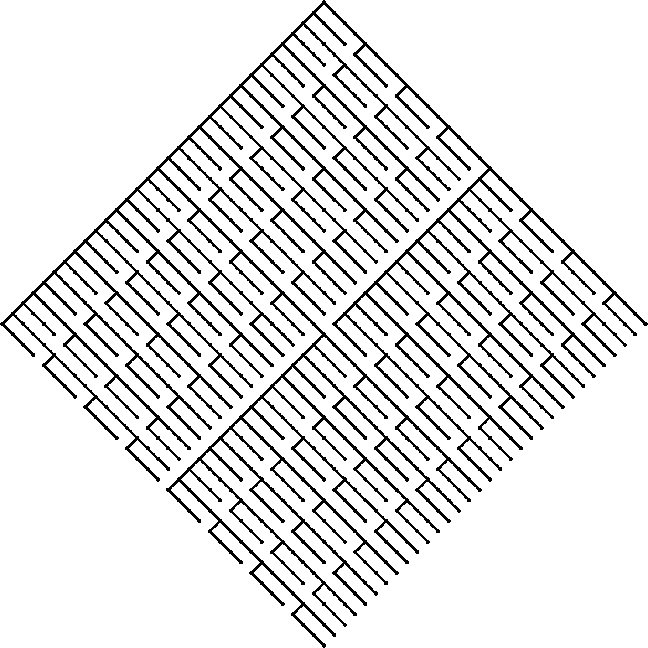
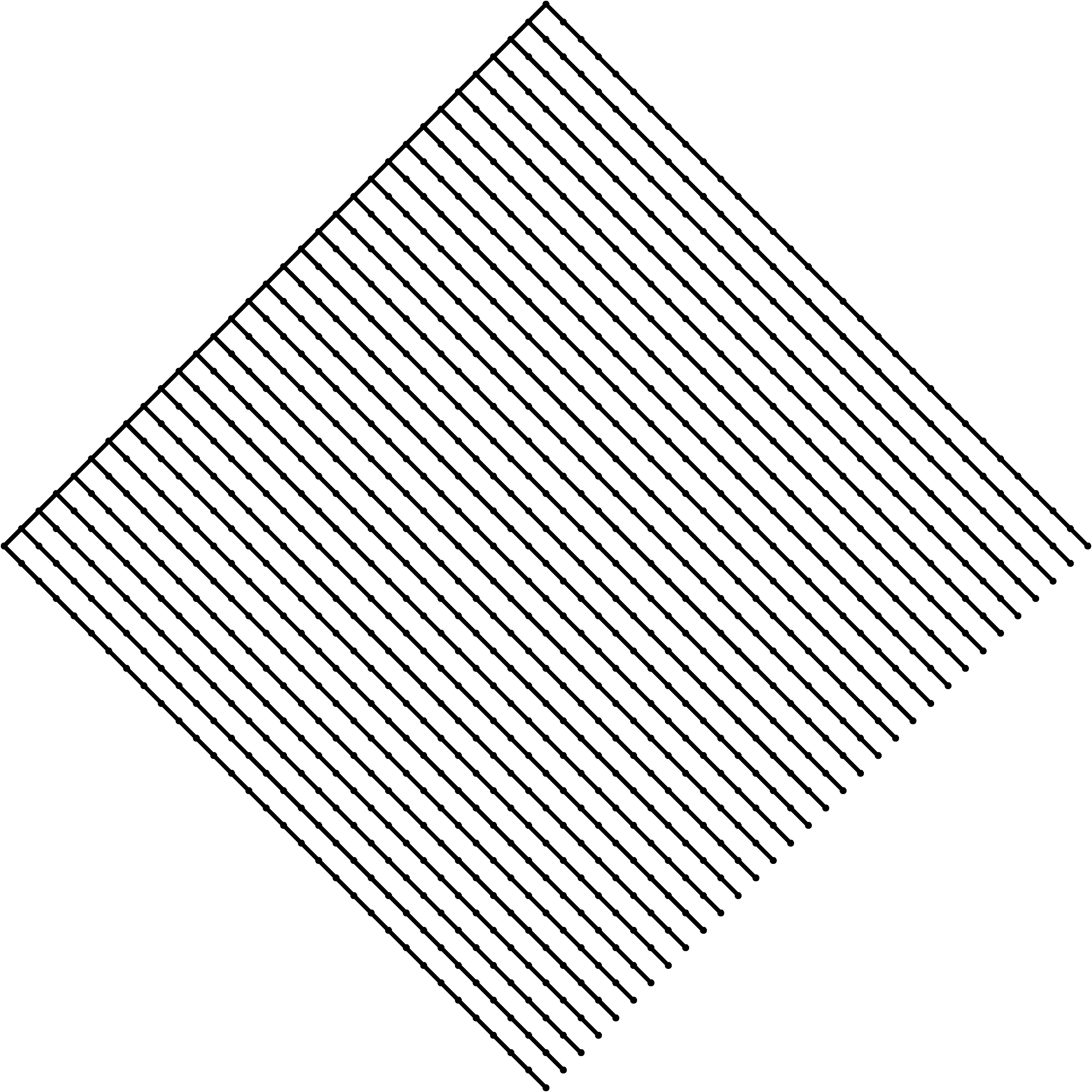
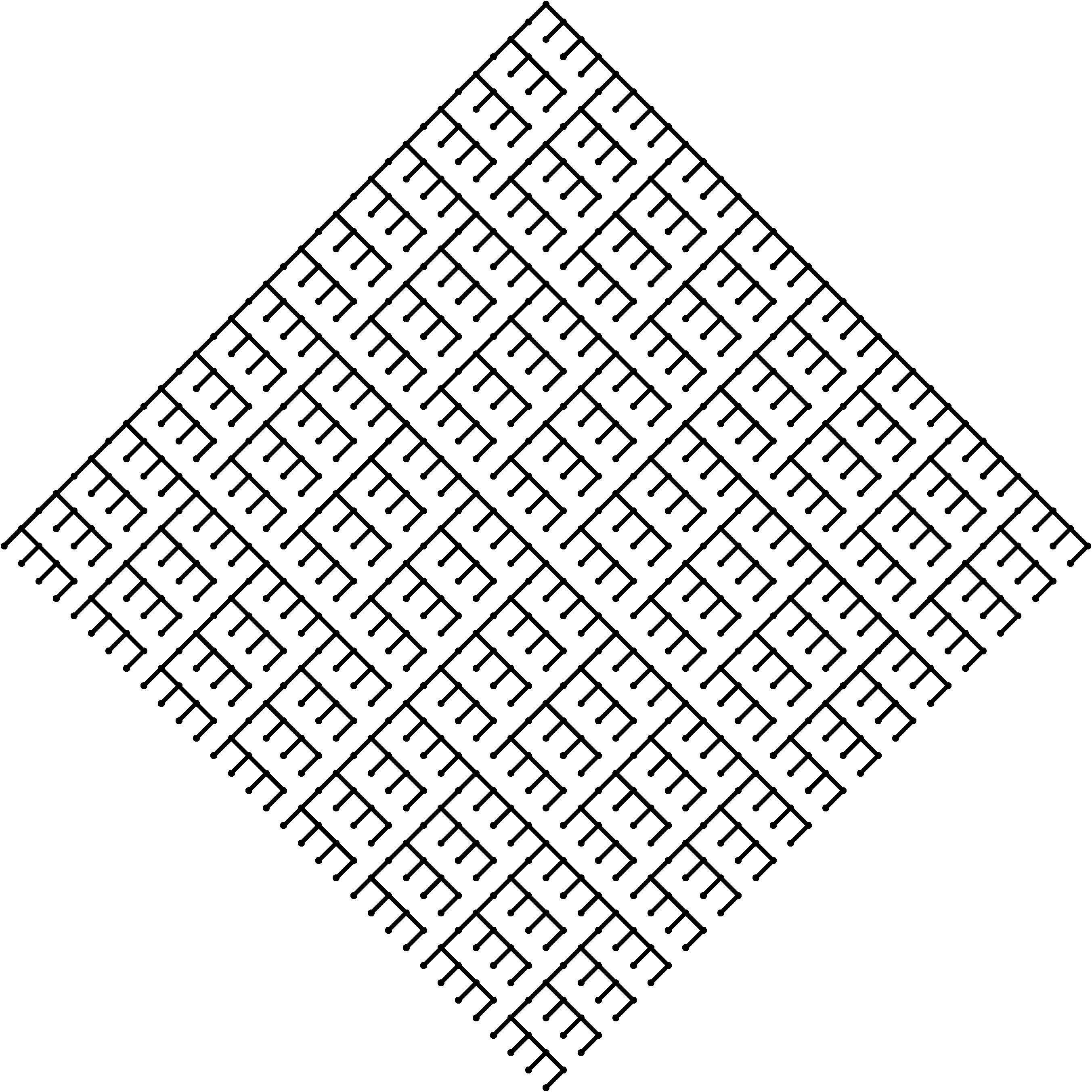
Figure 4: Simple butterfly trees with minimal height, $N=1{,}024$ nodes

Butterfly trees are BSTs formed using butterfly permutations. Due to the recursive constructions, butterfly trees have a unique shape determined by each permutation – so butterfly trees bridge the gap directly between the permutation weight random BST findings with the EBT studies (e.g., for $N$ node models, random BSTs have logarithmic average heights while EBTs have average heights proportional to square root[Dev86, FO82]). Butterfly trees were introduced and studied in depth in [PMZ25] with the focus on modeling the heights of butterfly trees, which we showed were at least $\sim N^{.585}$. We will study the complementary question regarding the HS. The height and HS are complementary statistics for binary trees, as the height is minimized precisely by the perfect binary trees and maximized by the identity permutation tree, whereas the HS has the inverse maximal and minimal relations to these tree models.

The first result we consider is the support of the HS for butterfly trees. Using one gluing operations, the support remained untouched (see Theorem 1), but the block construction impeded the capacity of larger HS as embedded perfect trees that combine both input trees need include the gluing edge. So we are now interested in what happens when we build up binary trees only using this operator? It ends up we substantially decrease the support:

Proposition 3.

Let $\mathcal{T}^{\operatorname{B}}=\mathcal{T}_{n}^{\operatorname{B}}$ be a butterfly tree with $N=2^{n}$ nodes. Then

$$\operatorname{HS}(\mathcal{T}^{\operatorname{B}})\leq{\lfloor\log_{4}N\rfloor}.$$

This inequality is sharp.

Proof.

We use induction on $n$. Note we will prove a further result that a butterfly with maximal HS can only have a multiplicity of nodes with this maximal HS if $4\nmid N$. This is trivial for $n=0,1$ since $\operatorname{HS}(\mathcal{T}_{n}^{\operatorname{B}})=0={\lfloor\log_{4}N\rfloor}$, noting both nodes have HS 0 when $n=1$. Moreover, for $n=2$, then $\operatorname{HS}(\mathcal{T}^{\operatorname{B}})=0$ if $\mathcal{T}^{\operatorname{B}}=\mathcal{T}(\pi)$ for $\pi\in\{1234,4321,1243,4312\}$ and $\operatorname{HS}(\mathcal{T}^{\operatorname{B}})=1={\lfloor\log_{4}N\rfloor}$ for $\pi\in\{2134,2143,3421,3412\}$, and this maximal HS is achieved only by the root node within the entire tree.

Now assume the result holds for $n\geq 2$. It suffices to then consider $\mathcal{T}_{1}^{\operatorname{B}}\oplus\mathcal{T}_{2}^{\operatorname{B}}$ where $\mathcal{T}_{1}^{\operatorname{B}}$ has maximal HS, i.e., $\operatorname{HS}(\mathcal{T}_{1}^{\operatorname{B}})={\lfloor\log_{4}N\rfloor}$ (see Remark 1). We consider if $n$ is even first. Writing $n=2k$, then ${\lfloor\log_{4}N\rfloor}=k$. Since $\operatorname{HS}(\mathcal{T}_{1}^{\operatorname{B}})=k$ and the previous level $n-1$ could have maximal HS ${\lfloor\log_{4}N/2\rfloor}={\lfloor k-1/2\rfloor}=k-1$, then necessarily the root of $\mathcal{T}_{1}^{\operatorname{B}}$ is the only node in $\mathcal{T}^{\operatorname{B}}$ with HS $k$. Since then gluing $\mathcal{T}_{2}^{\operatorname{B}}$ to the end of a top edge of $\mathcal{T}_{1}^{\operatorname{B}}$ can at most extend a path from the root of $\mathcal{T}_{2}^{\operatorname{B}}$ to the composite root, which corresponds the root of $\mathcal{T}_{1}^{\operatorname{B}}$, and this path cannot then meet a path connecting nodes of HS $k$ from the opposite top edge from the gluing (since only the previous root had this maximal HS), then it follows $\operatorname{HS}(\mathcal{T}_{1}^{\operatorname{B}}\oplus\mathcal{T}_{2}^{\operatorname{B}})=k={\lfloor\log_{4}(2N)\rfloor}={\lfloor\log_{4}N+\frac{1}{2}\rfloor}$. (Note then the composite would then have a multiplicity of nodes with max HS $k$ along the gluing edge if the child butterfly tree was chosen to also have a maximal HS.)

Now if $n=2k+1$ is odd, then a similar construction can now consider $\mathcal{T}_{1}^{\operatorname{B}}$ that has a multiplicity of nodes with HS ${\lfloor\log_{4}N\rfloor}={\lfloor k+\frac{1}{2}\rfloor}=k$. We can then choose the gluing operation so that the gluing occurs on the opposite side of the parent edge with at least one additional node with HS $k$, and if we further choose the child butterfly tree to have HS $k$, then the merging rules then create a path from the child root to the composite root connecting nodes with HS $k$. This path then meets the existing path along the opposite top edge of the composite tree, so that then the composite root now has HS $k+1={\lfloor\log_{4}2N\rfloor}$. This completes the inductive step. ∎

This suggests in particular the average HS must then be smaller than the general EBT model with $N$ nodes, as this deterministic upper bound asymptotically matches the average value scaling for an EBT (see Equation 1). To recover information about the average HS for a general butterfly tree, we again need to consider the dynamics of the top edge of the gluing edges.

The nonsimple butterfly trees have the same modeling considerations as needed for the merging of two binary trees with one gluing operation (see Remarks 1 and 2), as these can then be modeled sufficiently by iteratively modeling the profiles of the top edges through each iterative step, that then determine the subsequent level top edge profiles. Although this outlines a direct line for analysis, we will abstain from modeling the nonsimple butterfly case in the present work, that remains a promising area for future research. So we will instead focus on the simple butterfly trees. Simple butterfly trees have significantly reduced complexity that now allows a full distributional description. We will first consider the case of uniform simple butterfly trees.

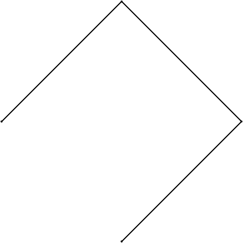
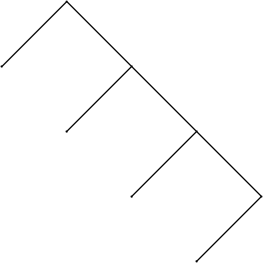
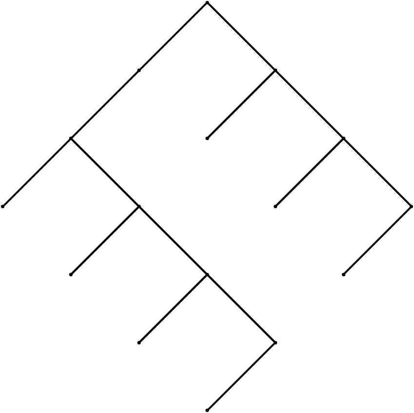
Figure 5: Intermediate simple butterfly trees $\mathcal{T}(10),\mathcal{T}(100),\mathcal{T}(1001)$ in building $\mathcal{T}(1001100101)$

3.1 Simple butterfly trees

Simple butterfly trees are formed using gluing operations on identical copies of the previous level tree, resulting in a fractal tree structure. Of particular note, then the simple butterfly trees necessarily fill out a rectangular lattice, where the height is achieved by the node at the bottom corner of this lattice [PMZ24]. (See Figure 4.) Our previous work established a full distributional description for the height of simple butterfly trees (see Equation 5). Similar other statistics are directly then outlined by studying this rectangular lattice, such as the maximal width or distribution of widths at a fixed depth. We are now interested in extending these results to consider the HS.

A key approach in modeling distributional properties of simple butterfly trees uses a compressed butterfly permutation representation of $\pi_{n}\in\operatorname{B}_{n,s}$. Since $\pi_{n}=\prod_{j=1}^{n}(1\ 2)^{x_{j}}$ for $x_{j}\in\{0,1\}$, then we can sufficiently capture the final form of $\pi_{n}$ using the $n$-bitstring ${\mathbf{x}}\in\{0,1\}^{n}$. This has the immediate advantage that one can compute some statistics for the corresponding permutation directly from the bitstring instead of first constructing the permutation.

Example 1.

The simple butterfly tree heights are a function of $X_{n}=\sum_{j=1}^{n}x_{j}$; for the uniform case, then $X_{n}\sim\operatorname{Bin}(n,1/2)$, as seen in Equation 5. This similarly derives the lengths of the longest increasing sequence (LIS) and longest decreasing sequence (LDS) [PMZ24], where $\operatorname{LIS}(\pi_{n})=2^{n-X_{n}}$ and $\operatorname{LDS}(\pi_{n})=2^{X_{n}}$.

Example 2.

The construction of the simple butterfly trees themselves are direct functions of the compressed butterfly permutation $n$-bitstrings ${\mathbf{x}}$, which we can write as $\mathcal{T}^{\operatorname{B}}({\mathbf{x}})$, where each bit indicates whether to glue two identical previous levels together by extending the top right (0) or top left (1) edge of the parent copy. Figure 5 shows the particular resulting simple butterfly trees for $\mathcal{T}^{\operatorname{B}}(0010011101)$, $\mathcal{T}^{\operatorname{B}}(0000011111)$, $\mathcal{T}^{\operatorname{B}}(1001100101)$. Figure 5 shows three intermediate forms $\mathcal{T}(10),\mathcal{T}(100),\mathcal{T}(1001)$ toward the right figure in Figure 4, $\mathcal{T}^{\operatorname{B}}(1001100101)$. (You can see the final figure in Figure 5 in each corner of the final figure in Figure 4.)

Remark 3.

Similarly, nonsimple butterfly permutations of length $N=2^{n}$ can be encoded using a compressed butterfly permutation now as $(N-1)$-bitstring. This aligns with an encoding from a complementary full $p$-ary rooted tree, with components corresponding to the local block rotations at that coordinate within the tree. This idea was implicitly important in the techniques in [AV05] by Abért and Virág, who resolve a long standing open question from Turán on the order of a random element from a $p$-Sylow subgroup using this correspondence. The non-identical butterfly trees used to build the next level tree, however, result in non-rectangular lattices: see Figure 6 for the nonsimple butterfly tree with 32 nodes, $\mathcal{T}^{\operatorname{B}}(1011000010010110001011110101010)$.

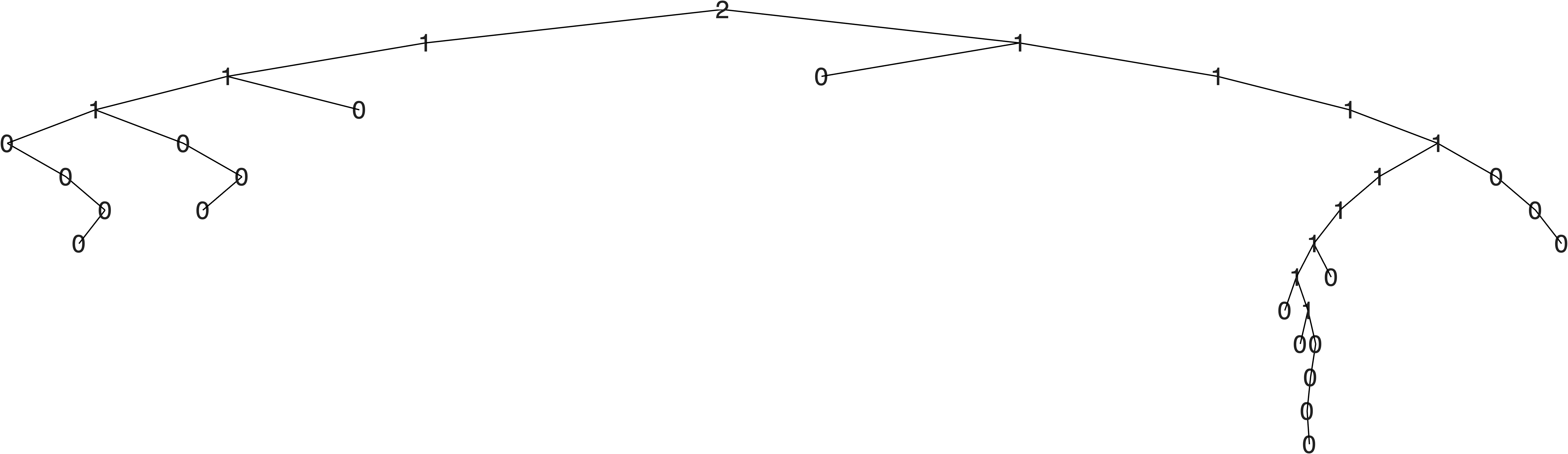
Figure 6: Nonsimple butterfly tree, $\mathcal{T}^{\operatorname{B}}(1011000010010110001011110101010)$, with HS labels, 32 nodes

A first step in establishing Theorem 2 is through outlining an explicit function of the compressed butterfly permutation that maps to the HS. For simple butterfly trees, we highlight the specific result from Remarks 1 and 2 that has the following implication: A simple butterfly tree $\mathcal{T}^{\operatorname{B}}({\mathbf{x}})$ with $N=2^{n}$ nodes, for ${\mathbf{x}}\in\{0,1\}^{n}$, is determined by a sequence of constructions of simple butterfly trees $\mathcal{T}({\mathbf{x}}(1:j))$ for $j=1:n$ (using MATLAB shorthand notation for sub-vectors formed by the first $j$ indices), where each $x_{j}$ determines whether the level $j$ gluing operator from the previous step extended the left or right top edge of the parent copy. This results in the HS of the level $n+1$ simple butterfly tree either:

• Matching the HS of the level $n$ simple butterfly tree if the gluing operator occurs along the same top edge that contains all nodes with maximal HS on the prior tree (this includes at least the root, and any additional such nodes can only occur along a top edge – and these can only occur exactly on either the top left or top right edge, as otherwise the root would have a left and right child with maximal HS, and hence it must have a higher HS), or

• Exceeds the HS of the level $n$ simple butterfly tree if the gluing operator occurs on the opposite edge that contains a multiplicity of nodes with maximal HS.

In particular, we note that an increase can thus occur at most every other intermediate butterfly tree. This follows since if the composite has an increase from the prior level, then only the root can have this maximal HS. So there is no multiplicity of nodes with maximal HS whenever such an increase occurs. Moreover, an increase can only occur if the prior two gluing operators have differing corresponding bits, i.e., $\texttt{xor}(x_{j},x_{j-1})=1$, where the exclusive OR function acts on two bit inputs $a,b\in\{0,1\}$ as

$$\texttt{xor}(a,b)=(a+b)\operatorname{mod}2.$$

If the prior two bits match in constructing the simple butterfly tree, then the rectangular lattice is formed by extending multiple copies of the prior form along the same top edge. (Figure 5 shows intermediate steps formed with alternating bits, so the first extension is on the top right edge followed by an extension on the top left edge.)

This directly results in the final realization of the HS for simple butterfly trees:

Proposition 4.

Let $\mathcal{T}^{\operatorname{B}}$ be a simple butterfly tree with $N=2^{n}$ nodes. Then for ${\mathbf{x}}\in\{0,1\}^{n}$, then

$$\operatorname{HS}(\mathcal{T}^{\operatorname{B}})=\sum_{j=1}^{n}X_{j},$$

where $X_{j}\in\{0,1\}$ satisfy $X_{1}=0$ and

$$X_{j}=\texttt{xor}(x_{j},x_{j-1})\cdot(1-X_{j-1}).$$

Note $X_{j}X_{j-1}=0$ by construction.

Proposition 4 is the main modeling tool for what remains with simple butterfly trees, which enables the corresponding very strong results we will outline. We will outline several corresponding directions based on this model, with the first consideration being for uniform simple butterfly trees.

3.1.1 Uniform simple butterfly trees

We will first explore some equivalent directions to derive the main results of Theorem 2 for the uniform case, when $x_{j}\sim\operatorname{Bern}(1/2)$ iid. Our goal is to establish three alternative proofs of the CLT from Theorem 2. The first two are derived directly from properties of the probability generating function (pgf), $\mathbb{E}[x^{\operatorname{HS}(\mathcal{T})}]$, which we will now outline.

First proof of Theorem 2

An immediate direction we will explore is through how Proposition 4 translates directly to a recurrence formula for the corresponding pgf for $\operatorname{HS}(\mathcal{T}^{\operatorname{B}})$ for uniform simple butterfly trees. This aligns with Flajolet’s original work on the register function for Cantor trees [Fla77]. In the uniform case, the problem reduces to enumerating the simple butterfly trees.

Let $f_{n}(k;j)$ denote the number of simple butterfly trees with HS equal to $k$ where the root is the only node with HS $k$ when $j=0$ (no multiplicity) and where at least 2 nodes (along either the top left or right edge) have HS $k$ when $j=1$ (with multiplicity). From the discussion preceding Proposition 4, it follows $f_{n}(k;j)$ satisfy recursion formulae:

$$f_{n+1}(k+1;0) =f_{n}(k;1)$$ (7)

$$f_{n+1}(k;1) =2\cdot f_{n}(k;0)+f_{n}(k;1).$$ (8)

This shows how a level $n$ butterfly tree can lead to an increase in HS for the next level only if there is a multiplicity of nodes with maximal HS, while otherwise either gluing operator yields a butterfly tree with matching HS. Now let

$$g_{n}(k)=f_{n}(k;0)+f_{n}(k;1)$$ (9)

denote the number of simple butterfly trees with HS $k$. Then

$$G_{n}(x)=2^{-n}\sum_{k=0}^{{\lfloor n/2\rfloor}}g_{n}(k)x^{k}$$

is the pgf for $\operatorname{HS}(\mathcal{T}^{\operatorname{B}})$ when $\mathcal{T}^{\operatorname{B}}$ is a uniform simple butterfly tree with $N=2^{n}$ nodes. The index running up to ${\lfloor n/2\rfloor}={\lfloor\log_{4}N\rfloor}$ follows directly from Proposition 3, since $n=\log_{2}N$.

The pgf determines the moments of $\operatorname{HS}(\mathcal{T}^{\operatorname{B}})$ since

$$\mathbb{E}[\operatorname{HS}(\mathcal{T}^{\operatorname{B}})^{k}]=\left.\left(x\frac{d}{dx}\right)^{k}G_{n}(x)\right|_{x=1}.$$ (10)

Our next goal will be to write $G_{n}(x)$ in a convenient recursive form:

Proposition 5.

Let $F_{n}(x)$ be the generating function for the number of simple butterfly trees with a multiplicity of nodes with max HS. Then $F_{0}(x)=0$, $F_{1}(x)=2$, and for $n\geq 1$

$$F_{n+1}(x)=2xF_{n-1}(x)+F_{n}(x).$$ (11)

Then $G_{n}(x)$ takes the form

$$G_{n}(x)=1+\frac{1}{2}(x-1)\sum_{k=0}^{n-1}2^{-k}F_{k}(x).$$ (12)

Moreover, for $1+8x\in\mathbb{C}\backslash(-\infty,0]$, then

$$G_{n}(x)=A(x)^{n}B(x)\cdot(1+O(|f(x)|^{n}))$$ (13)

where

$$A(x)=\frac{1}{4}(1+\sqrt{1+8x}),\quad B(x)=\frac{x(x-1)}{(A(x)-1)\cdot\sqrt{1+8x}},\quad f(x)=\frac{\sqrt{1+8x}-1}{\sqrt{1+8x}+1}.$$

Proof.

Let $H_{n}(x)$ denote the generating function for the number of simple butterfly trees whose root is the only node with maximal HS. Then

$$H_{n}(x) =\sum_{k\geq 0}f_{n}(k;0)x^{k},\qquad H_{0}(x)=1$$

$$F_{n}(x) =\sum_{k\geq 0}f_{n}(k;1)x^{k},\qquad F_{0}(x)=0,$$

and let

$$\tilde{G}_{n}(x):=H_{n}(x)+F_{n}(x),\qquad G_{n}(x)=2^{-n}\tilde{G}_{n}(x).$$

Using the recursions Equation 7 and Equation 8, we have

$$H_{n+1}(x)=xF_{n}(x),\qquad F_{n+1}(x)=2H_{n}(x)+F_{n}(x).$$

Hence, $F_{1}(x)=2$, and then Equation 11 follows by plugging in $H_{n}(x)=xF_{n-1}(x)$. Moreover, then

$$\tilde{G}_{n}(x)=xF_{n-1}(x)+F_{n}(x)$$

so that

$$\tilde{G}_{n+1}(x) =H_{n+1}(x)+F_{n+1}(x)=xF_{n}(x)+2H_{n}(x)+F_{n}(x)=2\tilde{G}_{n}(x)+(x-1)F_{n}(x)$$

Hence, we have

$$G_{n+1}(x)=G_{n}(x)+\frac{x-1}{2^{n+1}}F_{n}(x),$$

and so $G_{0}(x)=1$ and Equation 12 follows immediately.

For Equation 13, we first use the recurrence on the auxiliary function $F_{n}(x)$, with characteristic roots

$$r_{\pm}=r_{\pm}(x)=\frac{1}{2}\left(1\pm\sqrt{1+8x}\right),$$

to then write

$$F_{k}(x)=\frac{2x}{\sqrt{1+8x}}\left(r_{+}^{k}-r_{-}^{k}\right),$$

which is well-defined when $1+8x\notin(-\infty,0]$, i.e., avoiding the branch cut of the square root. Substituting this now into Equation 12 yields

$$G_{n}(x)=\frac{x(x-1)}{\sqrt{1+8x}}\cdot\sum_{k=1}^{n-1}\left[(r_{+}/2)^{k}-(r_{-}/2)^{k}\right]=\frac{x(x-1)}{\sqrt{1+8x}}\cdot\left[\frac{(r_{+}/2)^{n}-1}{(r_{+}/2)-1}-\frac{(r_{-}/2)^{n}-1}{(r_{-}/2)-1}\right].$$

The form Equation 13 follows immediately, noting $f(x)=-r_{-}(x)/r_{+}(x)$. ∎

This suffices to compute both the mean and variance of the HS of uniform simple butterfly trees.

Proposition 6.

Let $\mathcal{T}^{\operatorname{B}}$ be a uniform simple butterfly tree with $N=2^{n}$ nodes. Then

$$\mathbb{E}[\operatorname{HS}(\mathcal{T}^{\operatorname{B}})] =\frac{n}{3}-\frac{2}{9}+\frac{2}{9}\left(-\frac{1}{2}\right)^{n}=\log_{8}N+O(1),$$ (14)

$$\operatorname{Var}(\operatorname{HS}(\mathcal{T}^{\operatorname{B}})) =\frac{2}{27}n+\frac{2}{81}+\frac{4}{27}n\left(-\frac{1}{2}\right)^{n}+\frac{2}{81}\left(-\frac{1}{2}\right)^{n}-\frac{4}{81}\left(\frac{1}{4}\right)^{n}=\frac{2}{9}\log_{8}N+O(1).$$ (15)

Proof.

Since $n=\log_{2}N$, the final equalities in Equations 14 and 15 follow from $\frac{1}{3}n=\log_{8}N$. It remains to establish the first equalities.

From Proposition 5 and Equation 10,

$$\mathbb{E}[\operatorname{HS}(\mathcal{T}^{\operatorname{B}})]=G_{n}^{\prime}(1)=\frac{1}{2}\sum_{k=0}^{n-1}2^{-k}F_{k}(1).$$ (16)

Let $a_{k}=F_{k}(1)$. Then $a_{k+1}=2a_{k-1}+a_{k}$ with $a_{0}=0,a_{1}=2$. Solving the recurrence with characteristic polynomial $r^{2}=r+2$ gives

$$a_{k}=\frac{2}{3}(2^{k}-(-1)^{k}).$$

Substituting into Equation 16 yields the first equality in Equation 14.

For the variance, by Equation 10,

$$\operatorname{Var}(\operatorname{HS}(\mathcal{T}^{\operatorname{B}}))=G^{\prime\prime}_{n}(1)+G^{\prime}_{n}(1)-[G^{\prime}_{n}(1)]^{2}.$$ (17)

Again from Proposition 5,

$$G^{\prime\prime}_{n}(1)=\frac{1}{2}\sum_{k=0}^{n-1}2^{-k}F^{\prime}_{k}(1).$$ (18)

Let $b_{k}=F^{\prime}_{k}(1)$. Then $b_{0}=b_{1}=0$ and $b_{k+1}=b_{k}+2b_{k-1}+4a_{k-1}$. The homogeneous recurrence matches that of $a_{k}$, so

$$b_{k}=(A^{\prime}k+B^{\prime})2^{k}+(C^{\prime}k+D^{\prime})(-1)^{k}.$$

Substituting into Equation 18 yields

$$G_{n}^{\prime\prime}(1)=An^{2}+Bn+C+(Dn+E)\!\left(-\frac{1}{2}\right)^{n}.$$

Determining constants from initial values $G_{n}^{\prime\prime}(1)$ for $n=0,\dots,4$ gives

$$A=\frac{1}{9},\quad B=-\frac{11}{27},\quad C=\frac{8}{27},\quad D=\frac{8}{27},\quad E=-\frac{8}{27},$$

hence

$$G_{n}^{\prime\prime}(1)=\frac{1}{9}n^{2}-\frac{11}{27}n+\frac{8}{27}+\frac{8}{27}n\!\left(-\frac{1}{2}\right)^{n}-\frac{8}{27}\!\left(-\frac{1}{2}\right)^{n}.$$

Finally, substituting $G_{n}^{\prime}(1)$ from Equation 14 into Equation 17 gives the first equality in Equation 15. ∎

Proposition 6 suffices to establish the first main WLLN result in Theorem 2:

Corollary 1 (WLLN+).

Let $\mathcal{T}^{\operatorname{B}}$ be a uniform simple butterfly tree with $N=2^{n}$ nodes. Then for all $r\geq 1$, $(\operatorname{HS}(\mathcal{T}^{\operatorname{B}})/n)^{r}$ is uniformly integrable, and

$$\frac{\operatorname{HS}(\mathcal{T}^{\operatorname{B}})}{\log_{8}N}\xrightarrow[n\to\infty]{P}1,\qquad\frac{\operatorname{HS}(\mathcal{T}^{\operatorname{B}})}{\log_{8}N}\xrightarrow[n\to\infty]{L^{r}}1.$$

Proof.

The convergence in probability result follows from the Chebyshev inequality since

$$\operatorname{Var}(\operatorname{HS}(\mathcal{T}^{\operatorname{B}}))=\Theta(n)=o(n^{2})$$

from Proposition 6, while also $\mathbb{E}[\operatorname{HS}(\mathcal{T}^{\operatorname{B}})]=\frac{1}{3}n+O(1)$. The uniformly integrable statement follows from the observation $\operatorname{HS}(\mathcal{T}^{\operatorname{B}})/n$ is compactly supported on $[0,1]$ for $n\geq 1$ by Proposition 3. Combining the convergence in probability and uniform integrability then yields the convergence in $L^{r}$. ∎

To complete the first proof of the CLT in Theorem 2, we invoke Hwang’s Quasi-power theorem [Hwa98]. This result establishes asymptotic normality for random variables whose moment generating function (mgf) is asymptotically of the form $\exp(W_{n}(t))$ for some analytic $W_{n}(t)$. In addition, it provides a Berry–Esseen type bound on the convergence rate:

Theorem 4 (Quasi-power theorem; Hwang, [Hwa98]).

Let $(\Omega_{n})_{n\geq 1}$ be a sequence of integer-valued random variables. Suppose the mgf $M_{n}(t)=\mathbb{E}[\exp(t\Omega_{n})]$, satisfies the asymptotic expression:

$$M_{n}(t)=\exp(W_{n}(t))\cdot(1+O(\kappa_{n}^{-1})),$$

the $O$-error term being uniform in $|t|\leq\tau$, $t\in\mathbb{C}$, $\tau>0$, where

$$W_{n}(t)=u(t)\psi(n)+v(t),$$

where $u$ and $v$ analytic on $|t|\leq\tau$, independent of $n$, with $u^{\prime\prime}(0)\neq 0$, $\psi(n)=\omega_{n}(1)$ and $\kappa_{n}=\omega_{n}(1)$. Then

$$\mathbb{P}\left(\frac{\Omega_{n}-u^{\prime}(0)\psi(n)}{\sqrt{u^{\prime\prime}(0)\psi(n)}}\leq x\right)=\Phi(x)+O\left(\frac{1}{\sqrt{\psi(n)}}+\frac{1}{\kappa_{n}}\right)$$

uniformly with respect to $x\in\mathbb{R}$, for $\varphi(t)=\frac{1}{\sqrt{2}\pi}e^{-t^{2}/2}$ the probability density function (pdf) and $\Phi(x)=\int_{-\infty}^{x}\varphi(t)\ dt$ the cumulative distribution function (cdf) of a standard normal $\mathcal{N}(0,1)$.

We now have sufficient tools for the first proof of the CLT from Theorem 2:

Corollary 2 (CLT).

Let $\mu_{n}=\mathbb{E}\operatorname{HS}(\mathcal{T}^{\operatorname{B}})$ and $\sigma_{n}^{2}=\operatorname{Var}(\operatorname{HS}(\mathcal{T}^{\operatorname{B}}))$. Then

$$Z_{n}:=\frac{\operatorname{HS}(\mathcal{T}^{\operatorname{B}})-\mu_{n}}{\sigma_{n}}\xrightarrow[n\to\infty]{d}\mathcal{N}(0,1),\qquad\sup_{x}\left|\mathbb{P}\left(Z_{n}\leq x\right)-\Phi(x)\right|=O\left(\frac{1}{\sqrt{n}}\right).$$

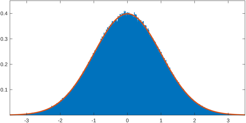
Figure 7: Histogram of normalized HSs for simple butterfly trees with $2^{100{,}000}\approx 9.99\cdot 10^{30{,}102}$ nodes, $1{,}000{,}000$ trials

Proof.

Using Proposition 5, we have the mgf $M_{n}(t)=G_{n}(e^{t})$ takes the form

$$M_{n}(t)=\exp({W_{n}(t)})\cdot(1+O(\rho^{n}))$$ (19)

where $W_{n}(t)=u(t)n+v(t)$, for $\varphi(n)=n$, and $u(t)$ and $v(t)$ analytic on $|t|\leq\tau$ for any

$$\tau<\tau^{*}=\sqrt{\log^{2}8+\pi^{2}}\approx 3.76745,$$

with

$$u(t)=\log\left(\frac{1}{2}r_{+}(e^{t})\right)=\log\left(\frac{1}{4}(1+\sqrt{1+8e^{t}})\right).$$

In particular, setting $\tau=1$ works, so that we can set

$$\kappa_{n}^{-1}=\max_{|t|=1}|f(e^{t})|^{n}=|f(e)|^{n},\qquad|f(e)|=\frac{\sqrt{1+8e}-1}{\sqrt{1+8e}+1}\approx 0.65333.$$

Now, expanding $u(t)$ near 0 gives:

$$u(t)=\frac{t}{3}+\frac{t^{2}}{27}-\frac{t^{3}}{343}-\frac{t^{4}}{8748}+\cdots,$$ (20)

with then $u^{\prime}(0)=1/3$ and $u^{\prime\prime}(0)=2/27$. By Proposition 6, we have $\mathbb{E}[\operatorname{HS}(\mathcal{T}^{\operatorname{B}})]\sim u^{\prime}(0)n$ and $\operatorname{Var}(\operatorname{HS}(\mathcal{T}^{\operatorname{B}}))\sim u^{\prime\prime}(0)n$. It follows then $\operatorname{HS}(\mathcal{T}^{\operatorname{B}})$ satisfies the hypotheses of Theorem 4, which then yields the final results along with Slutsky’s theorem (noting $O\left({{\psi(n)}}^{-1/2}+|f(e)|^{n}\right)=O(n^{-1/2})$). ∎

Remark 4.

An immediate consequence from Corollary 2 is a Local Limit Theorem (LLT):

$$\mathbb{P}(\operatorname{HS}(\mathcal{T}^{\operatorname{B}})=k)=\frac{1}{\sigma_{n}}\varphi(\frac{k-\mu_{n}}{\sigma}_{n})+O\left(\frac{1}{\sqrt{n}}\right),\qquad k-\mu_{n}=O(\sigma_{n}).$$

The $O(n^{-1/2})$ error term can be sharpened to $O(n^{-1})$ using an Edgeworth-expansion, along with the third cumulant $\kappa_{3}=-\frac{6}{343}n\cdot(1+o(1))=\Theta(n)$ from Equation 20.

Remark 5.

Recall $n=\log_{2}N$. So the convergence in Corollary 2 is very slow in terms of the number of nodes $N$ of the butterfly tree.

Exploiting the fact the HS can be computed very efficiently directly from the compressed butterfly permutation (see Remark 8), we can compute the HS for a large number of samples of large simple butterfly trees. Figure 7 displays a histogram of $10^{5}$ trials of HSs of uniform simple butterfly trees with $N=2^{1{,}000}\approx 1.07\cdot 10^{301}$ (computed in under 42 seconds). The sample mean and variance for these samples was 334.1214 and 73.9379, that aligned well with the true mean and variance of about 334.1111 and 74.0988 from Proposition 6.

Together, these now complete the proof of Theorem 2:

Proof of Theorem 2.

Combine Corollaries 1 and 2. ∎

Second proof of Theorem 2

The second proof of the CLT from Theorem 2 (i.e., Corollary 2) uses properties of the zeros of the pgf $G_{n}(t)$. This parallels Harper’s original proof of the CLT for the Stirling distribution $\Upsilon_{n}$, $\mathbb{P}(\Upsilon_{n}=k)=|s(n,k)|/n!$ for $s(n,k)$ the Stirling numbers of the first kind, which model the number of cycles of a uniform permutation [Har67]. Beyond their role in limit theorems, the zero patterns of $G_{n}(x)$ are of independent interest, connecting to classical and modern work on the zero distributions of generating functions and orthogonal polynomials [Sze75, PW13].

As adopted from [LW07], we first introduce a few additional definitions regarding zeros of real polynomials. Suppose two real polynomials $f(x)$ and $g(x)$ have only real zeros $\{s_{i}\},\{r_{j}\}$, written in non-increasing order. Then we say $g$ alternates left of $f$ if $\deg(f)=\deg(g)=n$ and

$$s_{n}\leq r_{n}\leq s_{n-1}\leq\cdots\leq s_{1}\leq r_{1}.$$

We say $g$ interlaces $f$ if $\deg(f)=\deg(g)+1=n$ and

$$r_{n}\leq s_{n-1}\leq\cdots\leq s_{1}\leq r_{1}.$$

We then write $g\preceq f$ to indicate $g$ alternates left of or interlaces $f$. If the inequalities above are strict, then we write $g\prec f$ to indicate $g$ strictly alternates left of or interlaces $f$.

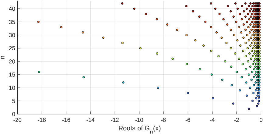
Figure 8: Interlacing roots of $G_{n}(x)$ for successive levels

We now state our result for the zeros of $G_{n}$:

Proposition 7.

For $n\geq 2$, $G_{n}(x)$ has only real negative zeros and $G_{n}\prec G_{n+1}$.

Remark 6.

Proposition 7 is illustrated explicitly in Figure 8, which plots successive zeros in $[0,20]$ for $G_{n}(x)$ for $n\leq 42$. This figure show the zeros clearly interlacing in the figure, additional structure is explicit relating each of the largest zero for even $n$ as well as the smallest zero for odd $n$, along with intermediate rankings across indices. Future work can explore this relationship in more detail.

Before going forward with the proof, we first state a useful theorem that captures when real-rootedness and interlacing are preserved under linear combinations. This is found as Theorem 2.1 in [LW07]:

Theorem 5 (Liu-Wang, [LW07]).

Let $F,f,g$ be three real polynomials that satisfy:

1. $F(x)=a(x)f(x)+b(x)g(x)$, such that $a(x)$ and $b(x)$ are real polynomials, with $\deg(F)=\deg(f)$ or $\deg(F)=\deg(f)+1$.

2. $f$, $g$ have only real zeros, and $g\preceq f$.

3. $F$ and $g$ have leading coefficients of the same sign.

Suppose $b(r)\leq 0$ whenever $f(r)=0$. Then $F$ has only real zeros, and $f\preceq F$. Moreover, if $b(r)<0$ whenever $f(r)=0$, then $f\prec F$.

We now have sufficient tools to prove Proposition 7.

Proof of Proposition 7.

It is equivalent to interchange $G_{n}(x)$ and $\tilde{G}_{n}(x)=2^{n}G_{n}(x)$, as these have matching zeros. By Propositions 3 and 5, a simple inductive argument establishes $\deg(G_{n})={\lfloor n/2\rfloor}$ while the auxiliary function $F_{n}$ satisfies $\deg(F_{n})={\lfloor(n-1)/2\rfloor}$. In particular, we note $\deg(G_{n})=\deg(F_{n})$ or $\deg(G_{n})=\deg(F_{n})+1$ while $\deg(F_{n})=\deg(F_{n-1})$ or $\deg(F_{n})=\deg(F_{n-1})+1$ for $n\geq 1$. Similarly, a simple inductive argument yields both $F_{n}$ and $G_{n}$ have strictly positive coefficients for $n\geq 1$. Hence, by Descartes’ rule of signs, then $F_{n}$ and $G_{n}$ have zero positive roots. Since also $F_{n}(0)=\tilde{G}_{n}(0)=2$ for $n\geq 1$, then this yields if $F_{n}$ or $G_{n}$ have only real roots, then these roots are strictly negative.

We first establish the auxiliary function $F_{n}(x)$ satisfies $F_{n}$ has only real roots for $n\geq 2$, and $F_{n}\preceq F_{n+1}$ for $n\geq 3$. Starting with $F_{0}(x)=0$, $F_{1}(x)=2$, then by Equation 11 we have $F_{2}(x)=2$, $F_{3}(x)=4x+2$, $F_{4}(x)=8x+2$, and $F_{5}(x)=8x^{2}+12x+2$. So we have

$$\text{roots of $F_{3}$:}-1/2;\qquad F_{4}:-1/4;\qquad F_{5}:\approx-1.309,-.1910.$$

It follows $F_{3}\prec F_{4}$ and $F_{4}\prec F_{5}$, which each have only real negative roots. Now assume the result holds for $F_{m}$ for $5\leq m\leq n$. By Equation 11, then

$$F_{n+1}(x)=2xF_{n-1}(x)+F_{n}(x).$$

By Theorem 5, using $F=F_{n+1}$, $f=F_{n}$, $g=F_{n-1}$, $a(x)=1$ and $b(x)=2x$, we have $F_{n+1}$ has only real negative zeros, and $F_{n}\prec F_{n+1}$.

Next, we will show $G_{n}$ has only real negative roots for $n\geq 2$, and $F_{n}\prec G_{n}$ for $n\geq 3$: We first note

$$\text{roots of $G_{2}$}:-1;\qquad G_{3}:-1/3;\qquad G_{4}:\approx-2.281,-.219$$

It follows $G_{n}$ has real negative roots for $n=2,3,4$ and $F_{n}\prec G_{n}$ for $n=3,4$. Now assume the result holds for $4\leq m\leq n$. Writing

$$\tilde{G}_{n}(x)=xF_{n-1}(x)+F_{n}(x),$$

we then have the desired result by Theorem 5, using $F=\tilde{G}_{n}$, $f=F_{n}$, $g=F_{n-1}$, $a(x)=1$ and $b(x)=x$, using also the preceding result $F_{n}$ has only real negative roots and $F_{n}\prec F_{n_{1}}$ for $n\geq 3$.

Finally, writing

$$G_{n+1}(x)=G_{n}(x)+\frac{(x-1)}{2^{n+1}}F_{n}(x),$$

we then establish the main result for Proposition 7 using again Theorem 5, with now $F=G_{n+1}$, $f=G_{n}$, $g=F_{n}$, $a(x)=1$, $b(x)=(x-1)/2^{n+1}$. ∎

Now, we can employ a sufficient result that establishes a CLT for random variables whose pgf has zeros with negative real part. For instance, the following theorem is provided in [Hwa98] (as Corollary 2 there), with full proof in [HS02]:

Theorem 6 (Hwang [Hwa98]; Hwang-Steyaert, [HS02]).

Let $P_{n}(z)$ be the pgf of the random variable $\Omega_{n}$, $n\geq 1$. Suppose for each $n$, $P_{n}(z)$ is a polynomial whose roots are located in the half-plane $\Re(z)\leq 0$. If $\sigma_{n}^{2}=\operatorname{Var}(\Omega_{n})\xrightarrow[n\to\infty]{}\infty$ and $\mu_{n}=\mathbb{E}[\Omega_{n}]$, then

$$\mathbb{P}\left(\frac{\Omega_{n}-\mu_{n}}{\sigma_{n}}\leq x\right)=\Phi(x)+O\left(\frac{1}{\sqrt{\sigma}_{n}}\right),\qquad x\in\mathbb{R}.$$

This yields an alternative proof of Corollary 2 (and hence of Theorem 2):

Proof of Corollary 2.

Combine Proposition 7 and Theorem 6. ∎

Remark 7.

Proposition 7 gives a stronger result than what is needed in Theorem 6, as the zeros of $G_{n}(z)$ are in fact real. This opens promising directions for studying the associated limiting zero measures, with potential connections to analogues of the Hermite or Chebyshev zero distributions. Further progress might include identifying explicit asymptotic densities for these measures or establishing universality classes for interlacing zeros in related polynomial families.

The remaining proof of the CLT from Theorem 2 will be pursued in the more general setting of random (non-uniform) simple butterfly trees in Section 3.2. Before shifting focus to the general model, we will establish additional properties for the uniform case.

Further properties of the uniform model

We collect several additional properties of the HS for uniform simple butterfly trees. These include an explicit distribution, asymptotic approximations, binomial identities, and symmetry invariances.

(a) Explicit distribution.

We begin by deriving a closed form for the probability mass function (pmf). This can be derived by a direct combinatorial argument.

Proposition 8.

Let $\mathcal{T}^{\operatorname{B}}$ be a uniform simple butterfly tree with $N=2^{n}$ nodes. Then

$$p_{n}(k):=\mathbb{P}(\operatorname{HS}(\mathcal{T}^{\operatorname{B}})=k)=2^{k-n}\cdot\left[\binom{n-k}{k}+\binom{n-k-1}{k}\right],\qquad k=0,1,\ldots,{\lfloor n/2\rfloor}.$$

Proof.

Working directly from Proposition 4, the HS can be computed from the compressed butterfly permutation ${\mathbf{x}}\in\{0,1\}^{n}$: increments occur precisely when $\texttt{xor}(x_{j},x_{j-1})=1$ and when $X_{j-1}=0$, so computing $\operatorname{HS}$ reduces to counting the number of nonconsecutive bit flips in ${\mathbf{x}}$.

For $n=0$ we clearly have $\operatorname{HS}(\mathcal{T}^{\operatorname{B}})=0$, so $p_{0}(0)=1$. For $n\geq 1$, the only way to have no bit flips is if ${\mathbf{x}}$ is the all-zeros or all-ones vector, yielding $p_{n}(0)=2^{1-n}$. At the other extreme, if $n$ is even, the maximum number of flips $n/2$ occurs when each adjacent pair $(x_{2j-1},x_{2j})$ is either $(0,1)$ or $(1,0)$. There are $2^{n/2}$ such strings, giving $p_{n}(n/2)=2^{-n/2}$ for even $n$ and zero otherwise.

For the intermediate cases, suppose there are exactly $k$ nonconsecutive bit flips. Each flip occurs at a pair $(x_{2j-1},x_{2j})\in\{(0,1),(1,0)\}$, giving $2^{k}$ options. The placement of flips depends on whether the last flip occurs before or at the final bit $x_{n}$.

• Case 1 (last flip before $x_{n}$): after removing the $2k$ bits used by the flips, there remain $n-2k$ bits. To ensure at least one trailing bit after the last flip, we separate one bit at the end, leaving $n-2k-1$ to distribute into $k+1$ “gaps” before and between flip locations. By stars-and-bars, this gives $\binom{n-k-1}{k}$ choices, each contributing a factor of $2$ for the trailing bits (all-zeros or all-ones).

• Case 2 (last flip at $x_{n}$): after removing the $2k$ bits used by flips, the remaining $n-2k$ bits are distributed among the $k$ gaps before each flip. This yields $\binom{n-k-1}{k-1}$ possibilities.

Adding the two cases gives

$$2^{k}\cdot\left[2\binom{n-k-1}{k}+\binom{n-k-1}{k-1}\right]=2^{k}\cdot\left[\binom{n-k}{k}+\binom{n-k-1}{k}\right],$$

using Pascal’s identity. Dividing by $2^{n}$ completes the proof. ∎

(b) Asymptotics.

The explicit pmf enables local limit approximations. For example, when $n-k-1\geq k$, we can simplify

$$p_{n}(k)\;=\;2^{k-n}\cdot\frac{2n-3k}{\,n-2k\,}\cdot\binom{n-k}{k}.$$

If $k=\lfloor\mathbb{E}\operatorname{HS}(\mathcal{T}^{\operatorname{B}})\rfloor\approx n/3-1$ (see Proposition 6), then

$$p_{n}(k)\;\approx\;\sqrt{\frac{27}{4\pi n}}\;\sim\;\frac{1}{\sqrt{2\pi}}\cdot\frac{1}{\sigma_{n}},$$

illustrating the LLT in Remark 4.

(c) Combinatorial identities.

Because Proposition 8 was derived independently of the pgf approach, the normalization condition $\sum_{k}p_{n}(k)=1$ yields binomial identities. For example,

$$2^{n}\;=\;\sum_{k=0}^{\lfloor n/2\rfloor}2^{k}\cdot\left[\binom{n-k}{k}+\binom{n-k-1}{k}\right].$$

For even $n=2m$, this reduces to

$$4^{m}=\sum_{k=0}^{m}2^{k}\cdot\left[\binom{2m-k}{k}+\binom{2m-k-1}{k}\right],$$

which admits hypergeometric reformulations. Similar manipulations applied to first and higher moments yield further identities.

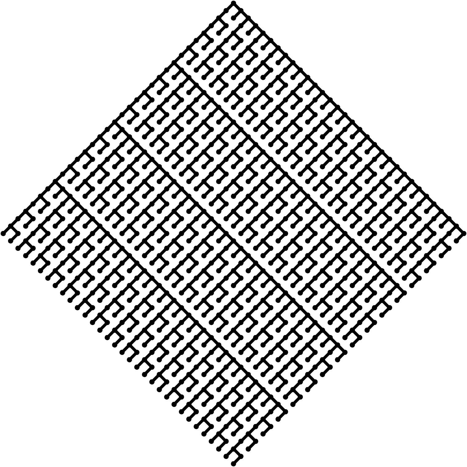
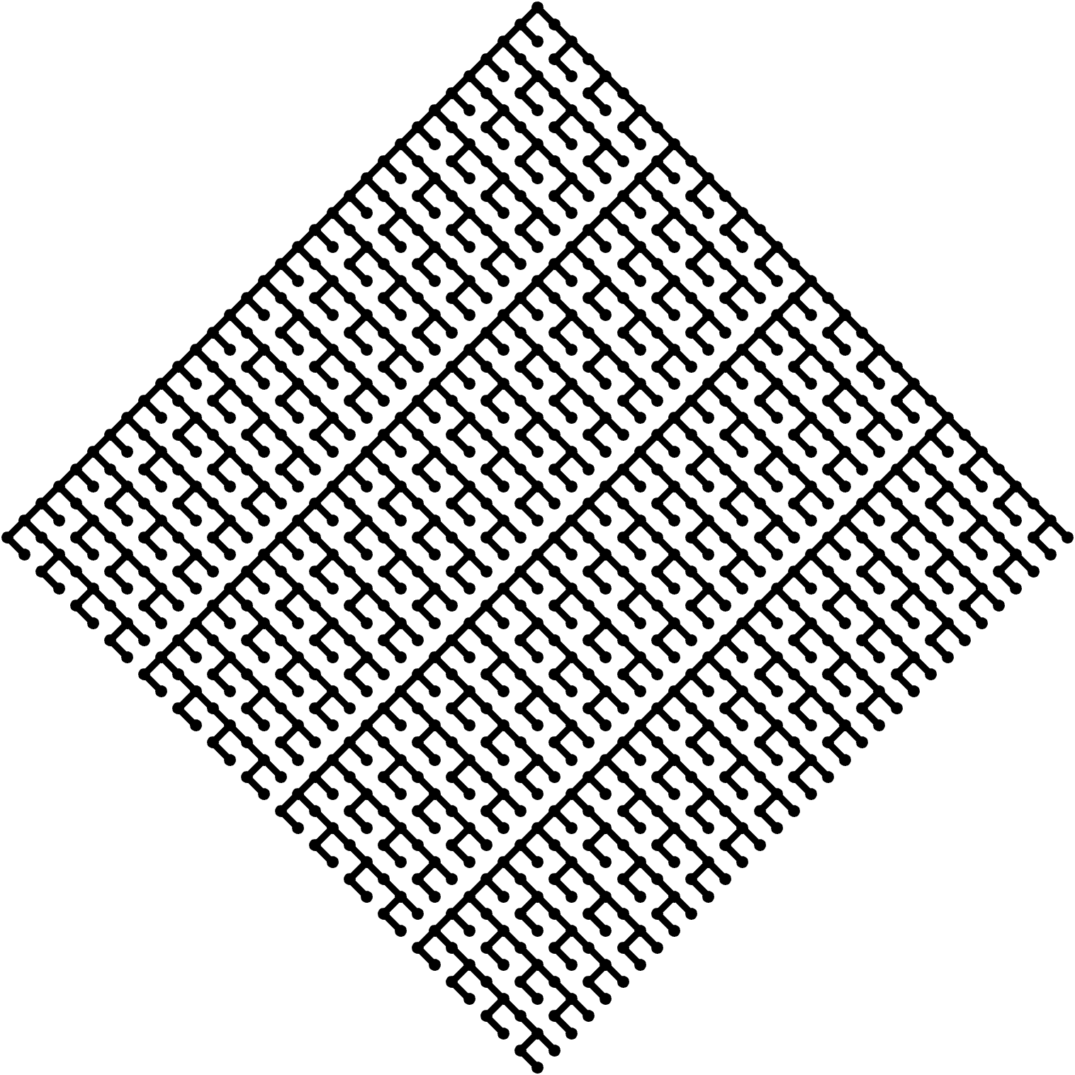
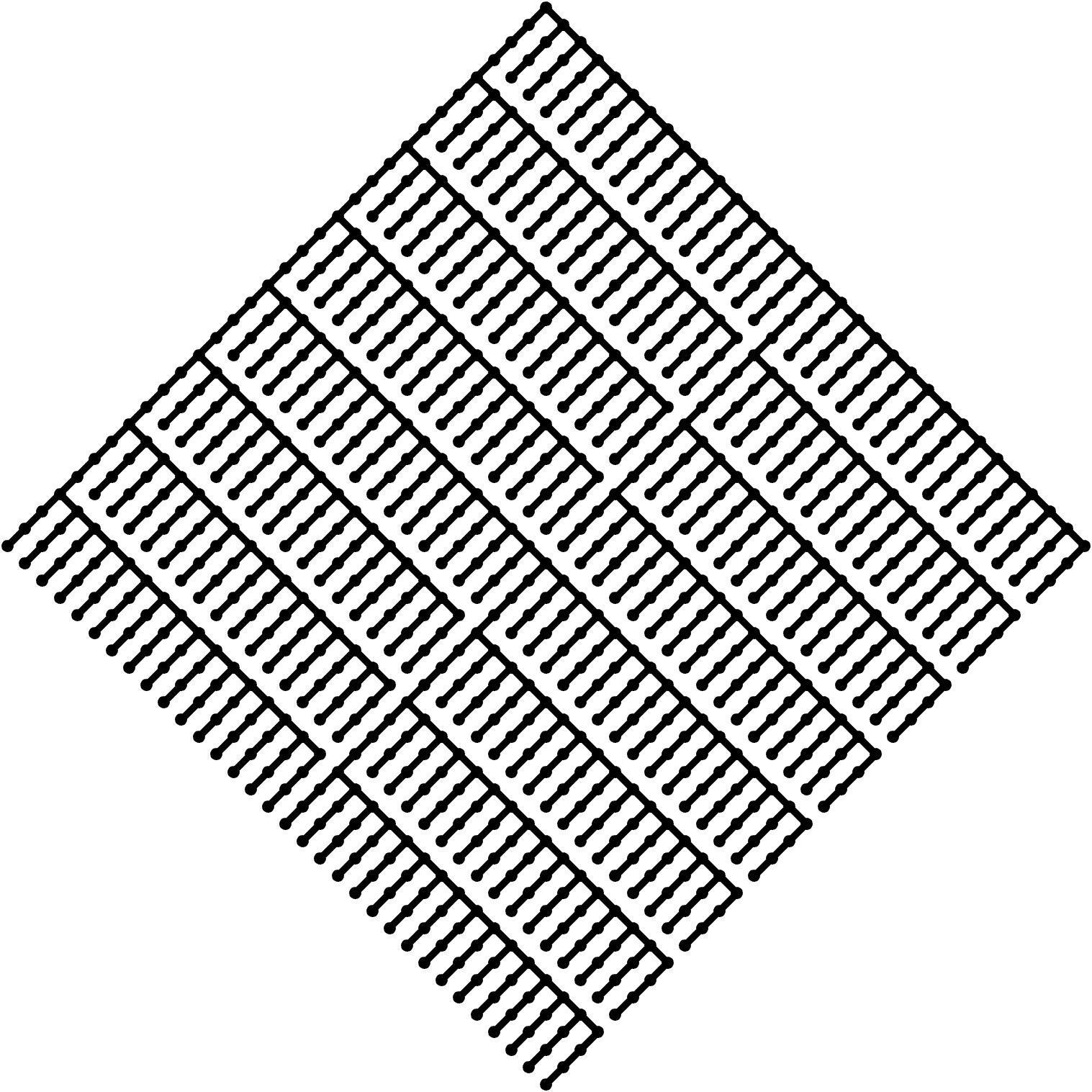
Figure 9: Simple butterfly tree $\mathcal{T}({\mathbf{x}})$ with ${\mathbf{x}}=1011000011$ and $\operatorname{HS}(\mathcal{T}^{\operatorname{B}}({\mathbf{x}}))=3$, along with the HS invariant butterfly trees formed using the inputs $\boldsymbol{1}-{\mathbf{x}}=0100111100$ and $\texttt{rev}({\mathbf{x}})=110000110$

(d) Symmetry invariances.

The HS is preserved under natural symmetries of the input string ${\mathbf{x}}\in\{0,1\}^{n}$, as seen in Figure 9.

• Complement invariance. By Proposition 4, we immediately have

  $$\operatorname{HS}(\mathcal{T}^{\operatorname{B}}({\mathbf{x}}))=\operatorname{HS}(\mathcal{T}^{\operatorname{B}}(\boldsymbol{1}-{\mathbf{x}})),$$

  since the map ${\mathbf{x}}\mapsto\boldsymbol{1}-{\mathbf{x}}$ simply interchanges each $\oplus/\ominus$ merge, which corresponds to reflecting the butterfly tree $\mathcal{T}^{\operatorname{B}}$ across the root.

• Reversal invariance. Less immediate is invariance under reversal,

  $$\texttt{rev}({\mathbf{x}}):\quad x_{j}\mapsto x_{n-j+1}.$$

  From Proposition 4, computing $\operatorname{HS}(\mathcal{T}^{\operatorname{B}}({\mathbf{x}}))$ amounts to counting the number of nonconsecutive bit flips in ${\mathbf{x}}$. Define ${\mathbf{y}}\in\{0,1\}^{n-1}$ by $y_{j}=\texttt{xor}(x_{j+1},x_{j})$. Then $\operatorname{HS}(\mathcal{T}^{\operatorname{B}}({\mathbf{x}}))$ is determined by the lengths of the maximal runs of $1$s in ${\mathbf{y}}$: if these have lengths $k_{1},\dots,k_{\ell}$, then

  $$\operatorname{HS}(\mathcal{T}^{\operatorname{B}}({\mathbf{x}}))\;=\;\sum_{j=1}^{\ell}\left\lceil\frac{k_{j}}{2}\right\rceil.$$ (21)

  Since the multiset of run-lengths $(k_{1},\dots,k_{\ell})$ is invariant under reversal, the HS number is preserved. Equivalently, reversal corresponds to constructing the binary tree in the opposite order—starting from the outer block structure and then expanding nodes according to subsequent bits.

Remark 8.

Equation 21 also yields a direct algorithm for computing $\operatorname{HS}(\mathcal{T}^{\operatorname{B}}({\mathbf{x}}))$ in $O(n)$ time, an exponential improvement over the standard $O(N)$ run time for computing HS on binary trees with $N$ nodes. This algorithm (and a recursive variant) are applicable to both uniform and non-uniform input distributions. The direct method was used to compute the $10^{5}$ sampled HS numbers for uniform simple butterfly trees with $N=2^{1{,}000}\approx 1.0715\cdot 10^{301}$ nodes, in Figure 7.

3.2 Random simple butterfly trees

We now turn to the non-uniform model, where the input bits are sampled independently with arbitrary bias $p\in(0,1)$. Recall from Proposition 4 that the sequence of Bernoulli increments $X_{j}$, which can be expressed recursively in terms of the input bits. This admits a convenient Markov chain formulation.

Proposition 9.

Let $(x_{j})_{j\geq 1}$ be iid $\operatorname{Bern}(p)$, and set $X_{0}=0$. Define recursively

$$X_{j}\;=\;\texttt{xor}(x_{j},x_{j-1})\cdot(1-X_{j-1}),\qquad j\geq 1.$$

Then the process

$$M_{j}\;=\;(x_{j},\,x_{j-1},\,X_{j-1})\in\{0,1\}^{3}$$

is an $8$-state time-homogeneous Markov chain.

Proof.

By construction, $M_{j}$ is determined from $M_{j-1}$ and a fresh sample $x_{j}\sim\operatorname{Bern}(p)$. Writing $q=1-p$, we have the transition

$$M_{j}=(a,b,c)\;\mapsto\;(\xi,a,f(a,b,c)),\qquad\xi\sim\operatorname{Bern}(p),$$

where $f(a,b,c)=\texttt{xor}(a,b)\cdot(1-c)$. Thus the law of $M_{j}$ depends only on $M_{j-1}$, establishing the Markov property.

Label the states $(a,b,c)$ by $k=4a+2b+c+1$ (binary encoding). The resulting transition matrix is

$$P^{(p)}=\begin{bmatrix}q&0&0&0&p&0&0&0\\ q&0&0&0&p&0&0&0\\ 0&q&0&0&0&p&0&0\\ q&0&0&0&p&0&0&0\\ 0&0&0&q&0&0&0&p\\ 0&0&q&0&0&0&p&0\\ 0&0&q&0&0&0&p&0\\ 0&0&q&0&0&0&p&0\end{bmatrix}.$$

This corresponds to the following transition digraph:

The associated transition digraph is strongly connected, so the chain is irreducible. A direct computation of the characteristic polynomial,

$$\det(\lambda I-P^{(p)})=\lambda^{5}(\lambda-1)(\lambda^{2}-pq),$$

shows that the chain is aperiodic whenever $pq\neq 0$. Since the chain has a finite state space, it admits a unique stationary distribution $\boldsymbol{\pi}$, given explicitly by

$$\boldsymbol{\pi}^{\top}=\frac{1}{1-pq}\left[q^{3},\ p^{2}q^{2},\ p^{2}q,\ pq^{3},\ pq^{2},\ p^{3}q,\ p^{3},\ p^{2}q^{2}\right].$$

∎

Remark 9.

For the uniform case, recall $X_{j}$ is a function of $x_{1},\ldots,x_{j-1}$, where $x_{j}\sim\operatorname{Bern}(1/2)$ iid. Then $\texttt{xor}(x_{j},x_{j-1})\sim\operatorname{Bern}(1/2)$ is also independent of $X_{j}$. (These remain dependent if $p\neq 1/2$.) It follows $X_{j}$ forms a 2 state time-homogeneous Markov chain, with transition matrix and digraph

$$P=\begin{bmatrix}1/2&1/2\\ 1&0\end{bmatrix}$$

and stationary distribution $\boldsymbol{\pi}^{\top}=[2/3,1/3]$. This additionally yields an alternative approach to computing the nonasymptotic mean and variance of $\operatorname{HS}(\mathcal{T}^{\operatorname{B}})$ from Proposition 6.

This then enables upgrades of Theorem 2 to Theorem 3. The first upgrade we will outline is the WLLN to SLLN by now framing the HS of a simple butterfly tree as an additive functional of this Markov chain:

Proposition 10 (SLLN).

Let $\mathcal{T}^{\operatorname{B}}=\mathcal{T}^{\operatorname{B}}({\mathbf{x}})$ be a $p$-biased simple butterfly tree, with $x_{j}\sim\operatorname{Bern}(p)$. Then

$$\frac{1}{n}\operatorname{HS}(\mathcal{T}^{\operatorname{B}})\;\xrightarrow[n\to\infty]{\text{a.s.}}\;\mu_{p}:=\frac{pq}{1-pq}.$$

Proof.

Define $f:\{0,1\}^{3}\to\{0,1\}$ by $f(a,b,c)=\texttt{xor}(a,b)\cdot(1-c)$. Then $X_{j}=f(M_{j})$ and

$$\operatorname{HS}(\mathcal{T}^{\operatorname{B}})\;=\;\sum_{j=1}^{n}X_{j}.$$

Since $f$ is bounded and $(M_{j})$ is an irreducible, aperiodic Markov chain on a finite state space, the Ergodic theorem applies:

$$\frac{1}{n}\sum_{j=1}^{n}f(M_{j})\;\xrightarrow[n\to\infty]{\text{a.s.}}\;\mathbb{E}_{\pi}[f],$$

where $\pi$ is the stationary distribution. A direct calculation yields

$$\mathbb{E}_{\pi}[f]=\sum_{s\in\{0,1\}^{3}}f(s)\pi(s)=\boldsymbol{\pi}^{\top}{\mathbf{f}}=\frac{p^{2}q}{1-pq}+\frac{pq^{2}}{1-pq}=\frac{pq}{1-pq}.$$

Thus

$$\frac{1}{n}\operatorname{HS}(\mathcal{T}^{\operatorname{B}})\xrightarrow[n\to\infty]{\text{a.s.}}\mu_{p}.$$

∎

Remark 10.

For $p=\frac{1}{2}$, this gives $\mu_{1/2}=\frac{1}{3}$, recovering the uniform case.

Remark 11.

Recalling that $n=\log_{2}N$, Proposition 10 can be rewritten as

$$\frac{\operatorname{HS}(\mathcal{T}^{\operatorname{B}})}{\log_{2^{1/\mu_{p}}}N}\;\xrightarrow[n\to\infty]{\text{a.s.}}\;1,$$

with the uniform case $p=\frac{1}{2}$ yielding the normalized form recovering the $2^{1/\mu_{1/2}}=8$ scaling from Corollary 1. This convergence reflects the ergodicity of the underlying Markov chain $(M_{j})$, and shows that the uniform input distribution maximizes the mean growth rate of the HS number. (See Figure 10.)

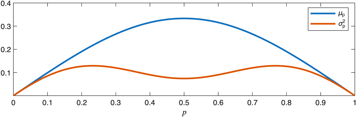
Figure 10: Plot of $\mu_{p},\sigma_{p}^{2}$

We now refine this limit theorem by establishing a third proof for the CLT Corollary 2. For additive functionals of finite, irreducible, aperiodic Markov chains, the asymptotic variance can be characterized through the Poisson equation

$$({\mathbf{I}}-P)g=h,$$ (22)

where $P$ is the transition matrix, $f$ is the observable and $h=f-\mu_{p}\mathbf{1}$ is the centered functional. (See [MT09] or [JH04] for further discussion.) Although $({\mathbf{I}}-P)$ is singular, the modified system

$$({\mathbf{I}}-P+\mathbf{1}\pi^{\top})g=h$$

is nonsingular and admits a unique solution $g$ orthogonal to $\pi$. For our setting, one obtains explicitly

$$g=(\mathbf{I}-P+\mathbf{1}\pi^{\top})^{-1}h=\frac{1}{8(1-pq)}\left[8p-5,\ 8p-5,\ 3,\ 8p-5,\ 3,\ 3-8p,\ 3-8p,\ 3-8p\right]^{\top}.$$ (23)

Then the variance constant

$$\sigma_{p}^{2}=\lim_{n\to\infty}\frac{1}{n}\operatorname{Var}\!\left[\sum_{j=1}^{n}X_{j}\right]$$

exists and is given by

$$\sigma_{p}^{2}=\operatorname{Var}_{\pi}[f]+2\sum_{k=1}^{\infty}\operatorname{Cov}(f(M_{1}),f(M_{k}))=\mathbb{E}_{\pi}\!\left[(h+2Pg)\odot h\right],$$

where $\odot$ denotes the elementwise Hadamard multiplication. In closed form,

$$\sigma_{p}^{2}=\frac{pq\left(1-3pq-2p^{2}q^{2}\right)}{(1-pq)^{3}}.$$ (24)

Remark 12.

Both $\mu_{p}$ and $\sigma_{p}^{2}$ are symmetric in $p$ and $q$, and depend only on $r:=pq$. Thus $\operatorname{HS}(\mathcal{T}^{\operatorname{B}}({\mathbf{x}}))\sim\operatorname{HS}(\mathcal{T}^{\operatorname{B}}({\mathbf{y}}))$ if $x_{j}\sim\operatorname{Bern}(p)$ and $y_{j}\sim\operatorname{Bern}(q)$, each iid, reflecting the natural symmetry of butterfly trees. Moreover, the variance-to-mean ratio

$$g(r):=\frac{\sigma_{p}^{2}}{\mu_{p}}=\frac{1-3r-2r^{2}}{(1-r)^{2}}$$

is strictly decreasing on $r\in[0,\frac{1}{4}]$, ranging from $g(0)=1$ to $g(1/4)=2/9$, which yields additionally $0\leq\sigma_{p}^{2}\leq\mu_{p}$ (see Figure 10). The variance is maximized at $p^{*}=\frac{1+\sqrt{13}}{6}\approx 0.7676$ and its symmetric counterpart $1-p^{*}$.

With this Markov process modeling for the HS of simple butterfly trees, we can additionally upgrade the CLT from Theorem 2 now to a full functional CLT. Figure 11 shows 60 sampled paths corresponding to $\operatorname{HS}(\mathcal{T}^{\operatorname{B}})$ for iid uniform simple butterfly trees with $n=10{,}000$, so that $N\approx 1.995\cdot 10^{3{,}010}$; this again utilized the efficient $O(n)$ sampling method referenced in Remark 8.

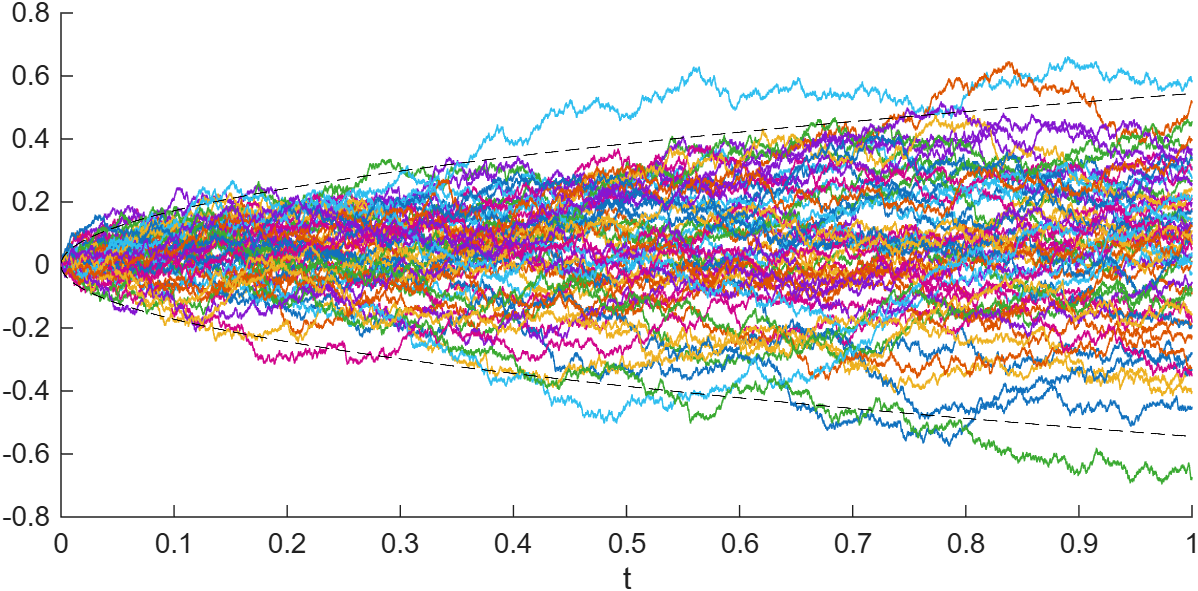
Figure 11: 60 sampled paths of $W_{n}(\frac{1}{2},t)$ with $n=10{,}000$, shown alongside the 95% confidence envelope bounded by $\pm 2\sigma_{1/2}\sqrt{t}=\pm\sqrt{\frac{8}{27}t}$ over $t\in[0,1]$.

Proposition 11 (Functional CLT).

Define the process

$$\operatorname{HS}(\mathcal{T}^{\operatorname{B}})(p,t)=\sum_{j=1}^{\lfloor nt\rfloor}X_{j},\qquad t\in[0,1]$$

for $X_{j}$ the dependent Bernoulli increments from Proposition 9. Then

$$W_{n}(p,t):=\sqrt{n}\left(\frac{1}{n}\operatorname{HS}(\mathcal{T}^{\operatorname{B}})(p,t)-t\mu_{p}\right)\xrightarrow[n\to\infty]{d}\sigma_{p}B(t),$$

where $B(t)$ is a standard Brownian motion for $t\in[0,1]$.

Proof.

Proposition 11 is a direct application of the functional CLT for Markov chains [MT09, Theorem 17.4], given the existence of a Poisson equation solution and the finiteness of $\sigma_{p}^{2}$. ∎

This now completes the proof of Theorem 3:

Proof of Theorem 3.

Combine Proposition 10 and Proposition 11. ∎

In particular, we can now provide a third alternative proof of Corollary 2 (and hence of Theorem 2).

Proof of Corollary 2.

Apply Proposition 11 with $t=1$, noting $\mu_{1/2}=\frac{1}{3}$ and $\sigma_{1/2}^{2}=\frac{2}{27}$. ∎

3.3 Nonsimple Butterfly Trees

Unlike the simple case, the picture for general (nonsimple) butterfly trees remains largely open. We established in Proposition 3 that

$$\operatorname{HS}(\mathcal{T})\;\leq\;\lfloor\log_{4}N\rfloor,$$

in sharp contrast to Cantor and EBT models, where the mean scales as $\log_{4}N$ but the support extends up to $\lfloor\log_{2}(N+1)\rfloor$. Empirically, the nonsimple model exhibits striking concentration: sampling $10{,}000$ butterfly trees of size $N=1{,}024$ yielded the frequency table

$$\begin{array}[]{c|c}\text{HS-number}&\text{Count}\\ \hline\cr 3&494\\ 4&9{,}040\\ 5&466\end{array}$$

with no samples below $3$. The resulting histogram (Figure 12) overlays these empirical frequencies with the exact pmf for simple butterfly trees from Proposition 8. The empirical statistics were

$$\widehat{\mathbb{E}}[\operatorname{HS}(\mathcal{T}^{\operatorname{B}})]\approx 3.9972,\qquad\widehat{\operatorname{Var}}(\operatorname{HS}(\mathcal{T}^{\operatorname{B}}))\approx 0.0960$$

(corresponding to a sample standard deviation $\approx 0.31$).

Two features stand out. First, although the theoretical upper bound for nonsimple butterfly trees is much smaller than the maximum of arbitrary binary trees ($\lfloor\log_{4}N\rfloor$ versus $\lfloor\log_{2}(N+1)\rfloor$), the observed mass is concentrated near the upper end of the available support (here, $4$ out of a maximum of $5$). Second, the variance is small, showing that the distribution is sharply concentrated around this level, potentially suggesting the variance may be bounded for general random butterfly trees.

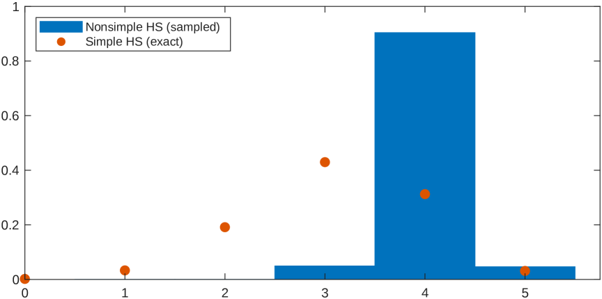
Figure 12: Histogram of HS for nonsimple butterfly trees ($N=1024$, $10{,}000$ samples) overlaid with exact probabilities for simple butterfly trees.

A rigorous explanation of these concentration effects would require a dynamic description of how successive gluing operations propagate along the top edges: each local gluing modifies the top-level block structure, and these updates accumulate across levels. A natural approach would be to model this evolution as a Markov or renewal process and then derive limit laws for its occupation statistics. Developing such a framework, and the corresponding fluctuation theorems, remains an open direction for future work.

Remark 13.

For nonsimple butterfly trees, the HS can be computed directly from the compressed permutation encoding in time linear in the bitstring length $N-1$, matching the standard $O(N)$ complexity of direct computation. Improvements may therefore only affect leading constants. By contrast, for simple butterfly trees the HS can be computed in $O(n)$ from their much shorter $n$-bit representation.

References

- [ABADK24] Louigi Addario-Berry, Marie Albenque, Serte Donderwinkel, and Robin Khanfir. Refined Horton–Strahler numbers I: a discrete bijection. arXiv preprint arXiv:2406.03025, 2024.
- [AV05] Miklós Abért and Bálint Virág. Dimension and randomness in groups acting on rooted trees. Journal of the American Mathematical Society, 18(1):157–192, 2005.
- [BBF+18] Frédérique Bassino, Mathilde Bouvel, Valentin Féray, Lucas Gerin, and Adeline Pierrot. The Brownian limit of separable permutations. The Annals of Probability, 46(4):2134–2189, 2018.
- [BBF+22] Frédérique Bassino, Mélanie Bouvel, Valentin Féray, Lucas Gerin, Mustazee Maazoun, and Adrien Pierrot. Scaling limits of permutation classes with a finite specification: a dichotomy. Advances in Mathematics, 405:108513, 2022.
- [BDR21] Anna Brandenberger, Luc Devroye, and Tommy Reddad. The Horton–Strahler number of conditioned Galton–Watson trees. Electronic Journal of Probability, 26:1–29, 2021.
- [BFS16] Guy E. Blelloch, Daniel Ferizovic, and Yihan Sun. Just join for parallel ordered sets. In Proceedings of the 28th ACM Symposium on Parallelism in Algorithms and Architectures (SPAA), pages 253–264, 2016.
- [BGS25] Jacopo Borga, Ewain Gwynne, and Xin Sun. Permutons, meanders, and SLE-decorated Liouville quantum gravity. Journal of the European Mathematical Society, 2025. Published online 12 June 2025, to appear.
- [BHSY23] Jacopo Borga, Nina Holden, Xin Sun, and Pu Yu. Baxter permuton and Liouville quantum gravity. Probability Theory and Related Fields, 186(3–4):1225–1273, 2023.
- [BLR14] M. Baboulin, X.S. Li, and F. Rouet. Using random butterfly transformations to avoid pivoting in sparse direct methods. In: Proc. of Int. Con. on Vector and Par. Proc., 2014.
- [Dev86] Luc Devroye. A note on the height of binary search trees. Journal of the ACM (JACM), 33(3):489–498, 1986.
- [DK95] Luc Devroye and Paul Kruszewski. A note on the Horton-Strahler number for random trees. Information Processing Letters, 56(2):95–99, 1995.
- [Fla77] Philippe Flajolet. Horton–Strahler number of a tree. Discrete Mathematics, 20(3):247–259, 1977.
- [FO82] Philippe Flajolet and Andrew Odlyzko. The average height of binary trees and other simple trees. Journal of Computer and System Sciences, 25(2):171–213, 1982.
- [FRV79] Philippe Flajolet, Jean-Claude Raoult, and Jean E. Vuillemin. The number of registers required for evaluating arithmetic expressions. Theoretical Computer Science, 9(1):99–125, 1979.
- [Har67] L. H. Harper. Stirling behaviour is asymptotically normal. Annals of Mathematical Statistics, 38:410–414, 1967.
- [HN22] Hiroaki Hirata and Atsushi Nunome. Parallel binary search tree construction inspired by thread-level speculation. In 2022 23rd ACIS International Summer Virtual Conference on Software Engineering, Artificial Intelligence, Networking and Parallel/Distributed Computing (SNPD-Summer), pages 74–81, 2022.
- [Hor45] Robert E. Horton. Erosional development of streams and their drainage basins: Hydrophysical approach to quantitative morphology. Geological Society of America Bulletin, 56(3):275–370, 1945.
- [HS02] Hsien-Kuei Hwang and Jean-Marc Steyaert. On the number of heaps and the cost of heap construction. In Brigitte Chauvin, Philippe Flajolet, Danièle Gardy, and Abdelkader Mokkadem, editors, Mathematics and Computer Science II: Algorithms, Trees, Combinatorics and Probabilities, Trends in Mathematics, pages 294–310. Birkhäuser, Basel, 2002.
- [Hwa98] H.-K. Hwang. On convergence rates in the central limit theorems for combinatorial structures. European Journal of Combinatorics, 19(3):329–343, 1998.
- [JH04] Galin L. Jones and James P. Hobert. Markov chain Monte Carlo: convergence and practical implementation. The American Statistician, 58(4):235–244, 2004.
- [Kem78] Robert Kemp. The expected Horton–Strahler number of a random tree. Discrete Mathematics, 23(1):37–52, 1978.
- [Khaara] Robin Khanfir. Fluctuations of the Horton–Strahler number of stable Galton–Watson trees. Annals of Probability, to appear. arXiv preprint arXiv:2401.13771.
- [Khaarb] Robin Khanfir. The Horton–Strahler number of Galton–Watson trees with possibly infinite variance. Annals of Applied Probability, to appear. arXiv preprint arXiv:2307.05983.
- [KP76] Jean-Pierre Kahane and Jacques Peyrière. Sur certaines martingales de Benoît Mandelbrot. Advances in Mathematics, 22(2):131–145, 1976.
- [Kru99] Paul Kruszewski. A note on the Horton-Strahler number for random binary search trees. Information Processing Letters, 69(1):47–51, 1999.
- [KRV20] Antti Kupiainen, Rémi Rhodes, and Vincent Vargas. Integrability of Liouville theory: Proof of the DOZZ formula. Annals of Mathematics, 191(1):81–166, 2020.
- [LLD24] Neil Lindquist, Piotr Luszczek, and Jack Dongarra. Generalizing random butterfly transforms to arbitrary matrix sizes. ACM Transactions on Mathematical Software, 50(4):1–23, 2024.
- [LW07] Lily L. Liu and Yi Wang. A unified approach to polynomial sequences with only real zeros. Advances in Applied Mathematics, 38(4):542–560, 2007.
- [Maa20] Mustazee Maazoun. On the Brownian separable permuton. Combinatorics, Probability and Computing, 29(2):241–266, 2020.
- [Man74a] Benoît Mandelbrot. Multiplications aléatoires itérées et distributions invariantes par moyenne pondérée aléatoire. Comptes Rendus de l’Académie des Sciences de Paris, Série A, 278:289–292, 1974.
- [Man74b] Benoît Mandelbrot. Multiplications aléatoires itérées et distributions invariantes par moyenne pondérée aléatoire: quelques extensions. Comptes Rendus de l’Académie des Sciences de Paris, Série A, 278:355–358, 1974.
- [Man74c] Benoît B. Mandelbrot. Intermittent turbulence in self-similar cascades: divergence of high moments and dimension of the carrier. Journal of Fluid Mechanics, 62:331–358, 1974.
- [MM80] Amram Meir and John W. Moon. On Horton–Strahler numbers for random trees. Journal of the ACM, 27(2):384–392, 1980.
- [MT09] Sean P. Meyn and Richard L. Tweedie. Markov Chains and Stochastic Stability. Cambridge Mathematical Library. Cambridge University Press, 2nd edition, 2009.
- [Par95] D. Stott Parker. Random butterfly transformations with applications in computational linear algebra. Tech. rep., UCLA, 1995.
- [PM21] John Peca-Medlin. Numerical, spectral, and group properties of random butterfly matrices. PhD thesis, University of California, Irvine, 2021. ProQuest ID: PecaMedlin_uci_0030D_17221. Merritt ID: ark:13030m5ck4tnm.
- [PM24a] John Peca-Medlin. Complete pivoting growth of butterfly matrices and butterfly Hadamard matrices. arXiv preprint arXiv:2410.06477, 2024.
- [PM24b] John Peca-Medlin. Distribution of the number of pivots needed using Gaussian elimination with partial pivoting on random matrices. Ann. Appl. Probab., 34(2):2294–2325, 2024.
- [PMT23] John Peca-Medlin and Thomas Trogdon. Growth factors of random butterfly matrices and the stability of avoiding pivoting. SIAM J. Matrix Anal. Appl., 44(3):945–970, 2023.
- [PMZ24] John Peca-Medlin and Chenyang Zhong. On the longest increasing subsequence and number of cycles of butterfly permutations. arXiv preprint arXiv:2410.20952, 2024.
- [PMZ25] John Peca-Medlin and Chenyang Zhong. Heights of butterfly trees. arXiv preprint arXiv:2507.04505, 2025.
- [PW13] Robin Pemantle and Mark C. Wilson. Analytic Combinatorics in Several Variables, volume 140 of Cambridge Studies in Advanced Mathematics. Cambridge University Press, 2013.
- [RV14] Rémi Rhodes and Vincent Vargas. Gaussian multiplicative chaos and applications: A review. Probability Surveys, 11:315–392, 2014.
- [Sta15] Richard P. Stanley. Catalan Numbers, volume no. 153 of Cambridge Studies in Advanced Mathematics. Cambridge University Press, 2015. Contains 214 combinatorial interpretations of the Catalan numbers and additional exercises.
- [Str52] Arthur N. Strahler. Hypsometric (area-altitude) analysis of erosional topography. Geological Society of America Bulletin, 63(11):1117–1142, 1952.
- [Sze75] Gábor Szegő. Orthogonal Polynomials, volume 23 of American Mathematical Society Colloquium Publications. American Mathematical Society, Providence, RI, 4 edition, 1975.