Prioritizing Recurrent Services

Abstract

We study optimal scheduling in multi-class queueing systems with reentrance, where jobs may return for additional service after completion. Such reentrance creates feedback loops that fundamentally alter congestion dynamics and challenge classical scheduling results. We model two distinct dimensions of the reentrance behavior, the probability of return and the speed of return, and show that their product, the effective return rate, is the key statistic that governs optimal priorities. Our main result establishes a dichotomy: when the effective return rate of the smaller job class (the class with lower expected total workload) is lower, a fixed priority rule is optimal; when it is higher, fixed rules are suboptimal and the optimal policy must be state dependent. This characterization clarifies how reentrance changes the externalities that jobs impose on one another and provides structural guidance for designing scheduling policies.

1 Introduction

Service systems across many domains routinely face recurrent demand. In healthcare, patients return for follow-up visits; in call centers, customers make repeated support calls; and in professional services, clients revisit financial advisors. Service delivered today can therefore generate future arrivals, creating feedback loops that fundamentally reshapes system dynamics. Queueing models such as Erlang-R [Yom-Tov and Mandelbaum, 2014] explicitly capture these returns and show that ignoring them can lead to substantial biases in both analysis and decision making.

Our goal is to better control service systems with reentrance through smart prioritization and scheduling. Two observations motivate our study. First, recent advancements in predictive analytics and artificial intelligence make it increasingly feasible to classify jobs by their likelihood and timing of return. For example, in tech support, most setup or installation calls are resolved on the first attempt, but if they require a return, the follow-up typically happens within hours, whereas subscription clients almost always require support again, though only after weeks or months. Second, classical scheduling policies, such as the $c\mu$-rule [Mandelbaum and Stolyar, 2004] and shortest remaining processing time (SRPT) scheduling [Dong and Ibrahim, 2021], have been shown to be effective because they prioritize jobs that impose the least externality on others. This raises a natural question: in the presence of reentrance, where jobs differ in both their probability and speed of return, how should externality be quantified, and what scheduling policies remain effective?

We address this question using a fluid queueing model where a system manager dynamically allocates service capacity between two job classes (indexed by $i\in\{1,2\}$). The classes differ in their return probability ($r_{i}$) and return rate ($\gamma_{i}$). The system consists of a primary queue, where jobs line up for service and incur holding costs while waiting, and a virtual return queue, which tracks jobs that will reenter the system in the future. The objective is to minimize total holding costs in the primary queue. Our main research question is how optimal scheduling priorities should be structured in the presence of reentrance. We focus on whether the classical intuition of prioritizing “smaller” jobs with lower expected workload remains valid under reentrance, and whether optimal decisions are governed by fixed priority rules or require adaptation to system congestion.

Our main result provides a sharp characterization of the optimal scheduling policy; see Figure 1. Assume without loss of generality that $r_{1}<r_{2}$, so that class 1 represents the smaller jobs with lower expected total workload. For each class $i$, define the effective return rate as $\kappa_{i}=r_{i}\gamma_{i}$, which jointly captures how likely and how quickly work returns. We find that:

1. If $\kappa_{1}\leq\kappa_{2}$, a fixed priority policy is optimal: class 1 (the smaller jobs) should always be prioritized, independently of the system’s congestion level.

2. If $\kappa_{1}>\kappa_{2}$, no fixed priority policy is optimal. In this case, class 1 should be prioritized under heavy congestion, but priority should shift to class 2 when the system is lightly loaded.

Figure 1: Structure of the optimal scheduling policy

A key insight of our analysis is that reentrance changes the way jobs impose externalities on one another. In classical multi-class queues without returns, smaller jobs are always favored because they clear faster and permanently relieve congestion. With reentrance, however, serving jobs that are likely to return soon can offset this benefit. The effective return rate $\kappa_{i}=r_{i}\gamma_{i}$ captures this feedback and becomes the critical (though not exclusive) measure of class $i$’s externality. When $\kappa_{1}\leq\kappa_{2}$, the benefit of completing the smaller job still dominates, so always prioritizing class 1 remains optimal. When $\kappa_{1}>\kappa_{2}$, the optimal policy switches depending on the system load. When the system is already heavily loaded, the overriding concern is to drain work quickly to reduce holding costs. Class 1 jobs are smaller (since $r_{1}<r_{2}$), serving them clears backlog faster and immediately relieves congestion, even though they are prone to return soon. In this regime, the benefit of faster clearance outweighs the risk of quick reentries. Under light congestion, however, the immediate backlog is less pressing, and the main concern shifts to the future workload generated by today’s service. It is therefore better to prioritize class 2 with a lower effective return rate. In short, the effective return rate captures long-run feedback externalities, while the optimal policy balances them ($\kappa_{1}$ vs. $\kappa_{2}$) against the immediate externalities of leaving work unfinished ($r_{1}$ vs. $r_{2}$), which explains why fixed priority rules suffice in some regimes but fail in others.

2 Related Literature

First, our work is related to the literature on optimal scheduling in multi-class queues. One rich line of work emphasizes the power of simple index rules, such as the $c\mu$-rule and its extensions, and shows that these static priority rules can yield (near-)optimal performance in a wide range of queueing models [Smith et al., 1956, Van Mieghem, 1995, Mandelbaum and Stolyar, 2004, Atar et al., 2010, Long et al., 2020]. Complementing index policies, state-dependent rules that favor short jobs, such as SRPT and service-age-based variants, are known to minimize delay in a range of models [Schrage and Miller, 1966, Scully et al., 2018, Dong and Ibrahim, 2021, Ibrahim and Dong, 2026]. We contribute to this literature by showing how reentrance changes the notion of externality that underpins these rules. In our model, the product of return probability and return speed becomes the key statistic that governs whether fixed priority rules suffice or whether state dependence is essential.

Second, our work is related to the stream of literature on reentrant service systems. Classical Erlang-R models demonstrate that ignoring reentrance can lead to biased performance estimates and miscalibrated staffing, especially in healthcare [Yom-Tov and Mandelbaum, 2014, Armony et al., 2015]. More recent work shows that heterogeneous return dynamics can alter system stability and equilibrium [Barjesteh and Abouee-Mehrizi, 2021]. In addition, reentrance has been incorporated into diverse applications, including emergency department staffing with time-varying physician productivity [Ouyang et al., 2021], post-discharge hospital readmission prevention [Chan et al., 2025], community corrections placement [Gao et al., 2025], and customer-agent interactions in contact centers [Daw et al., 2025]. Collectively, these studies model reentrance as an important operational feature, but relatively little is known about how to optimally schedule recurrent jobs. We address this gap directly by showing how reentrance reshapes the notion of externalities in scheduling theory and by characterizing the structure of the optimal scheduling policy.

3 The Model

We consider a two-class fluid queueing system with reentrant jobs. The system is closed, with no external arrivals, and the objective is to optimally clear all existing workload. For each class $i$, work first enters a primary queue, where it receives service. After service completion, a fraction $r_{i}\in(0,1)$ of the work reenters the system by joining a virtual return queue. Jobs in the return queue depart at rate $\gamma_{i}>0$, at which point they rejoin the primary queue. Without loss of generality, we assume $r_{1}<r_{2}$, so that class 1 represents “smaller” jobs with a lower expected total work once the reentrance probability is taken into account.

The system manager has a total service capacity $\mu>0$, and dynamically allocates it between the two classes. Specifically, the system manager determines allocations $u(t)=(u_{1}(t),u_{2}(t))$, subject to $u_{i}(t)\geq 0$ and $u_{1}(t)+u_{2}(t)\leq 1$, $i\in\{1,2\}$, $t\geq 0$. If class $i$ receives a fraction $u_{i}(t)$ of capacity at time $t$, its primary queue is depleted at rate $\mu u_{i}(t)$.

At time $t$, let $q_{i}^{p}(t)$ denote the primary queue length of class $i$, $q_{i}^{r}(t)$ the amount of work in the return queue that will reenter in the future, and $q(t)=(q_{1}^{p}(t),q_{1}^{r}(t),q_{2}^{p}(t),q_{2}^{r}(t))$ the full system state. The system dynamics are given by

$$\dot{q}_{i}^{p}(t)=-\mu u_{i}(t)+\gamma_{i}q_{i}^{r}(t),\quad\dot{q}_{i}^{r}(t)=r_{i}\mu u_{i}(t)-\gamma_{i}q_{i}^{r}(t),\quad i=1,2.$$ (1)

We call a mapping $\psi$ an admissible policy if it prescribes allocations $u(t)=\psi(q(t))$ that maintain all queues nonnegative. A sample path of allocations $u$ is an optimal trajectory for given parameters and an initial condition if, among all admissible allocations, it achieves the minimal cumulative holding cost incurred by primary queues over a sufficiently long horizon $T$:

$$\int_{0}^{T}\left(q_{1}^{p}(t)+q_{2}^{p}(t)\right)\,dt.$$

A policy $\psi$ is said to be optimal for a given parameters if the resulting allocation trajectory $u(t)=\psi(q(t))$, $t\geq 0$, is an optimal trajectory for any initial condition. In general, we are interested in understanding how to construct optimal policies.

We say that the server prioritizes class $i\in\{1,2\}$ at state $q$ if (i) when $q_{i}^{p}>0$, the server devotes full capacity to class $i$; and (ii) when $q_{i}^{p}=0$, the server allocates enough capacity to keep $q_{i}^{p}$ empty.

A policy $\psi$ is a fixed priority policy if the server prioritizes one particular class at all states $q$, and a state-dependent policy otherwise. To emphasize, by state-dependent policy we mean one that is strictly state-dependent; fixed priority rules are not included as a special case.

4 Main Results

We now establish how reentrance shapes the structure of the optimal scheduling policy. The key determinant is the effective return rate $\kappa_{i}=r_{i}\gamma_{i}$, which reflects not only how much future workload class $i$ generates after service, but also the speed at which this workload returns to the system. Comparing $\kappa_{1}$ and $\kappa_{2}$ yields two distinct regimes.

Theorem 4.1.

The optimal scheduling policy satisfies:

1. If $\kappa_{1}\leq\kappa_{2}$, a fixed priority policy that always prioritizes class $1$ is optimal.

2. If $\kappa_{1}>\kappa_{2}$, no fixed priority policy is optimal, and the optimal policy is state-dependent.

We complement Theorem 4.1 with the following important observation, supported by extensive numerical experiments. In the regime where $\kappa_{1}>\kappa_{2}$, the optimal state-dependent policy exhibits at most one switch along any trajectory. Specifically, the policy prioritizes class 1 under heavy congestion and transitions to class 2 as the system clears. We next present a set of numerical experiments with parameters from the region $\kappa_{1}>\kappa_{2}$ where no fixed priority policy is optimal. Figure 2 plots the evolution of the state $(q_{1}^{p},q_{2}^{p})$ under the optimal policy, starting from different initial conditions. We make two consistent observations: (i) when both queues are heavily loaded, the policy prioritizes class 1, but as the system clears, priority shifts to class 2; and (ii) along every trajectory, at most one switch of priority occurs. In other words, smaller jobs dominate prioritization under high congestion, but their rapid returns eventually make it more efficient to prioritize larger jobs as the system clears.

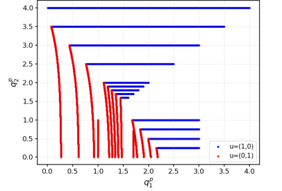
Figure 2: Optimal state trajectories when $\kappa_{1}>\kappa_{2}$ ($r_{1}=0.2$, $r_{2}=0.8$, $\gamma_{1}=2$, $\gamma_{2}=0.2$, $\mu=2$, $q^{r}(0)=0$)

Importantly, our results illustrate how reentrance changes the nature of externalities in scheduling. In classical queues without reentrance, smaller jobs always impose less externality, since they leave the system quickly and permanently free capacity. With reentrance, completing a job may regenerate demand, so a higher effective return rate $\kappa_{i}$ reflects a stronger future externality. However, the optimal rule is not determined by comparing $\kappa_{1}$ and $\kappa_{2}$ alone. Under heavy congestion, the main externality is the immediate delay from large backlogs, and prioritizing the smaller jobs (class 1) best alleviates this burden, even if they are more likely to return soon. Under light congestion, the immediate backlog is less pressing, and the dominant externality becomes the feedback created by future returns. In that regime, it is optimal to prioritize the class with the smaller $\kappa_{i}$. In a nutshell, $\kappa_{i}$ quantifies future externalities, but the optimal prioritization balances them against the more myopic externality of delaying work clearance. This tradeoff explains why fixed priority rules fail when $\kappa_{1}>\kappa_{2}$ and state dependence becomes necessary.

To conclude, we numerically demonstrate the value of state-dependent policies by comparing the objective values of the optimal state-dependent policy with those of the two fixed priority rules. In Table 1, the “FP-1 gap” column reports the relative performance loss from always prioritizing class 1, while the “FP-2 gap” column does the same for class 2. The results show that giving fixed priority to class 1 can be close to optimal when the parameters are near the boundary where $\kappa_{1}=\kappa_{2}$, but becomes increasingly suboptimal as class 2 returns more slowly. Conversely, fixed priority to class 2 performs poorly near the boundary but improves steadily as its return rate decreases.

$\gamma_{2}$	FP-1 gap	FP-2 gap
0.05	7.35%	0.01%
0.10	5.02%	0.01%
0.20	0.89%	0.67%
0.30	0.03%	4.68%
0.40	0.01%	10.16%
0.50	0.00%	16.01%

Table 1: Improvement over fixed priority rules ($r_{1}=0.2$, $r_{2}=0.8$, $\gamma_{1}=2$, $\mu=2$, $q^{p}(0)=2$, $q^{r}(0)=0$)

Appendix A Proof of Theorem 4.1

In this section, we present the proof of Theorem 4.1. Section A.1 shows that the fixed-priority policy that always prioritizes class 1 is optimal when $\kappa_{1}\leq\kappa_{2}$. Section A.2 establishes that no fixed-priority policy can be uniformly optimal for all initial states $q_{0}$ when $\kappa_{1}>\kappa_{2}$, using proof by contradiction.

A.1 Proof of Theorem 4.1 Part (1)

To prove Part (1) of Theorem 4.1, we proceed in two steps. First, we rewrite the control problem by expressing the state trajectories $q_{i}^{p}(t)$ and $q_{i}^{r}(t)$ in integral form. This representation yields a convenient kernel formulation of the objective, highlighting how the control enters linearly over time. Second, we apply Pontryagin’s Minimum Principle. By analyzing the Hamiltonian and its coefficients, we show that whenever $\kappa_{1}\leq\kappa_{2}$, the Hamiltonian is minimized by allocating as much capacity as feasibly possible to class 1 at every state. This corresponds exactly to the fixed priority policy that always prioritizes class 1, thereby proving its optimality.

We now begin the proof by expressing $q_{i}^{p}(t)$ and $q_{i}^{r}(t)$ in integral form. By (1), for any feasible allocation $u=(u_{1},u_{2})$ (i.e., allocation that satisfies $0\leq u_{i}\leq 1$ and $u_{1}+u_{2}\leq 1$), we obtain

$$q_{i}^{r}(t) =e^{-\gamma_{i}t}q_{i,0}^{r}+r_{i}\mu\int_{0}^{t}e^{-\gamma_{i}(t-s)}u_{i}(s)\,ds,$$

$$q_{i}^{p}(t) =q_{i,0}^{p}+\int_{0}^{t}-\mu u_{i}(s)+\gamma_{i}q_{i}^{r}(s)\,ds$$

$$=q_{i,0}^{p}-\mu\int_{0}^{t}u_{i}(s)\,ds+\int_{0}^{t}\gamma_{i}q_{i}^{r}(s)\,ds$$

$$=q_{i,0}^{p}-\mu\int_{0}^{t}u_{i}(s)\,ds+(1-e^{-\gamma_{i}t})q_{i,0}^{r}+\gamma_{i}r_{i}\mu\int_{0}^{t}\left[\int_{s}^{t}e^{-\gamma_{i}(x-s)}\,dx\right]u_{i}(s)\,ds$$

$$=q_{i,0}^{p}-\mu\int_{0}^{t}u_{i}(s)\,ds+(1-e^{-\gamma_{i}t})q_{i,0}^{r}+\gamma_{i}r_{i}\mu\int_{0}^{t}\frac{1}{\gamma_{i}}\left[1-e^{-\gamma_{i}(t-s)}\right]u_{i}(s)\,ds.$$

Define the kernel $k_{i}(\tau)=\mu[(r_{i}-1)-r_{i}e^{-\gamma_{i}\tau}]$, $\tau\geq 0$, so that the primary queue length admits the compact representation

$$q_{i}^{p}(t)=q_{i,0}^{p}+(1-e^{-\gamma_{i}t})q_{i,0}^{r}+\int_{0}^{t}k_{i}(t-s)u_{i}(s)\,ds.$$

Next, let

$$K_{i}(\tau) =\int_{0}^{\tau}k_{i}(x)\,dx$$

$$=\mu\left[(r_{i}-1)\tau-\frac{r_{i}}{\gamma_{i}}(1-e^{-\gamma_{i}\tau})\right]$$

denote the cumulative kernel. Using Fubini’s Theorem, the finite-horizon objective can be expressed as

$$\int_{0}^{T}q_{1}^{p}(t)+q_{2}^{p}(t)\,dt =\sum_{i=1}^{2}\int_{0}^{T}\left[q_{i,0}^{p}+(1-e^{-\gamma_{i}t})q_{i,0}^{r}\right]\,dt+\sum_{i=1}^{2}\int_{0}^{T}\int_{0}^{t}k_{i}(t-s)u_{i}(s)\,ds\,dt$$

$$=C_{T}(q_{0})+\sum_{i=1}^{2}\int_{0}^{T}u_{i}(s)\left[\int_{s}^{T}k_{i}(t-s)\,dt\right]ds$$

$$=C_{T}(q_{0})+\sum_{i=1}^{2}\int_{0}^{T}u_{i}(s)K_{i}(T-s)\,ds,$$

where $C_{T}(q_{0})$ depends only on the initial state $q_{0}$ and horizon $T$. Therefore, minimizing the cumulative holding cost is equivalent to solving

$$\min_{u(\cdot)}\sum_{i=1}^{2}\int_{0}^{T}u_{i}(s)K_{i}(T-s)\,ds,$$

which reveals the problem as a linear functional of the control trajectory with weights $K_{i}(T-s)$. Importantly, the weight function $K_{i}(\cdot)$ has the following properties,

Lemma A.1.

Assume that $0<r_{1}<r_{2}<1$, for all $\tau\geq 0$, $K_{i}(\tau)\leq 0$. In particular, when $\kappa_{1}\leq\kappa_{2}$, $K_{1}(\tau)\leq K_{2}(\tau)$.

Proof. See Section A.3.

Recall from Section 3 that a policy $\psi$ is admissible if the allocations $u(t)=\psi(q(t))$ it prescribes keep all queues nonnegative. In particular, when the primary queue of class $i$ is empty ($q_{i}^{p}(t)=0$), we require $\dot{q}_{i}^{p}(t)\geq 0$, which implies the constraint $\mu u_{i}(t)\leq\gamma_{i}q_{i}^{r}(t)$. Collecting these conditions, the admissible allocation set at state $q$ is defined as

$$\mathcal{U}(q):=\left\{u:u_{1},u_{2}\geq 0,u_{1}+u_{2}\leq 1,\text{if }q_{i}^{p}=0,\text{then }\mu u_{i}\leq\gamma_{i}q_{i}^{r}\text{ for }i=1,2\right\}.$$ (2)

We now apply Pontryagin’s Principle to show that the fixed-priority policy prioritizing class 1 is optimal. For a fixed horizon $T>0$, the Hamiltonian is

$$\mathcal{H}(q,u,\lambda)=\sum_{i=1}^{2}q_{i}^{p}+\sum_{i=1}^{2}\lambda_{i}^{p}(-\mu u_{i}+\gamma_{i}q_{i}^{r})+\sum_{i=1}^{2}\lambda_{i}^{r}(r_{i}\mu u_{i}-\gamma_{i}q_{i}^{r}).$$

The costates satisfy $\dot{\lambda}_{i}^{p}(t)=-1$, $\dot{\lambda}_{i}^{r}(t)=-\gamma_{i}(\lambda_{i}^{p}(t)-\lambda_{i}^{r}(t))$, $\lambda_{i}^{p}(T)=\lambda_{i}^{r}(T)=0$. Solving backward gives us

$$\lambda_{i}^{p}(t)=T-t,\quad\lambda_{i}^{r}(t)=T-t-\frac{1}{\gamma_{i}}(1-e^{-\gamma_{i}(T-t)}).$$

So the coefficient of $u_{i}$ in $\mathcal{H}$ is

$$\mu(r_{i}\lambda_{i}^{r}(t)-\lambda_{i}^{p}(t))=\mu\left[r_{i}(T-t)-\frac{r_{i}}{\gamma_{i}}(1-e^{-\gamma_{i}(T-t)})-(T-t)\right]=K_{i}(T-t).$$

From Lemma A.1, for every $t\in[0,T)$, $K_{1}(T-t)\leq K_{2}(T-t)\leq 0$. By Pontryagin’s Principle, an optimal control $u^{*}(\cdot)$ must minimize the Hamiltonian pointwise over $\mathcal{U}(q^{*}(t))$, the admissible control set given in (2) to ensure control feasibility and state nonnegativity. Thus, the optimal allocation is

$$u_{1}^{*}(t)=\begin{cases}1,&\text{if }q_{1}^{p}(t)>0,\\ \min\{1,\gamma_{1}q_{1}^{r}(t)/\mu\}&\text{if }q_{1}^{p}(t)=0.\end{cases}\quad u_{2}^{*}(t)=\begin{cases}1-u_{1}^{*}(t),&\text{if }q_{2}^{p}(t)>0,\\ \min\{1-u_{1}^{*}(t),\gamma_{2}q_{2}^{r}(t)/\mu\}&\text{if }q_{2}^{p}(t)=0.\end{cases}$$

That is, the optimal policy allocates full capacity to class 1 whenever it has positive workload, and allocate just enough capacity to it to keep $q_{1}$ at 0 while maintaining feasibility. On the other hand, any leftover capacity will be given to class 2 whenever it has positive workload. This corresponds precisely to the fixed priority policy introduced in Section 3. Therefore, when $\kappa_{1}\leq\kappa_{2}$, the fixed priority policy that always prioritizes class 1 is optimal and obtains minimal cost under any $T$.∎

A.2 Proof of Theorem 4.1 Part (2)

Part (2) of Theorem 4.1 requires showing that no fixed-priority policy is optimal when $\kappa_{1}>\kappa_{2}$. Our strategy is to demonstrate that the two fixed-priority policies reverse their cost ranking under different initial conditions. Consider the family of initial states $q_{0}^{(\varepsilon)}=(q_{1}^{p},q_{2}^{p},q_{1}^{r},q_{2}^{r})=(\varepsilon,\varepsilon,0,0)$ with $\varepsilon>0$. For any parameters $(r_{1},r_{2},\gamma_{1},\gamma_{2})$ such that $r_{1}<r_{2}$ and $\kappa_{1}>\kappa_{2}$, we show that as $\varepsilon\to 0^{+}$, the policy that always prioritizes class 2 achieves a strictly lower cost than the policy that always prioritizes class 1. In contrast, as $\varepsilon\to\infty$, the inequality reverses. This proves that no single fixed-priority policy can minimize cost for all initial states $q_{0}$ in this regime.

Before analyzing the inequalities in the two asymptotic regimes, we first derive several key quantities needed for the proof. Suppose we implement the policy that prioritizes class $i$ exclusively. Let $t_{i}(\varepsilon)$ denote the first time at which the initial backlog of class $i$ is cleared (that is, when $q_{i}^{p}(t)$ reaches zero). Then, on interval $[0,t_{i}(\varepsilon))$, the primary and return queue lengths can be expressed in integral form as follows

$$q_{i}^{r}(t) =r_{i}\mu\int_{0}^{t}e^{-\gamma_{i}(t-s)}\,ds=\frac{r_{i}\mu}{\gamma_{i}}(1-e^{-\gamma_{i}t}),$$

$$q_{i}^{p}(t) =\varepsilon+\mu\int_{0}^{t}\left[(r_{i}-1)-r_{i}e^{-\gamma_{i}(t-s)}\right]\,ds=\varepsilon-\mu\left[(1-r_{i})t+\frac{r_{i}}{\gamma_{i}}(1-e^{-\gamma_{i}t})\right].$$

Therefore, $t_{i}(\varepsilon)$ is the unique solution to

$$\varepsilon=\mu\left[(1-r_{i})t_{i}(\varepsilon)+\frac{r_{i}}{\gamma_{i}}(1-e^{-\gamma_{i}t_{i}(\varepsilon)})\right].$$ (3)

Let $I_{i}(\varepsilon)$ denote the total cost accumulated by class $i$ over the interval $[0,t_{i}(\varepsilon))$,

$$I_{i}(\varepsilon)=\int_{0}^{t_{i}(\varepsilon)}q_{i}^{p}(t)\,dt=\varepsilon t_{i}-\frac{(1-r_{i})\mu}{2}t_{i}^{2}(\varepsilon)-\frac{r_{i}\mu}{\gamma_{i}}\left({t_{i}-\frac{1-e^{-\gamma_{i}t_{i}(\varepsilon)}}{\gamma_{i}}}\right).$$

Once the backlog of class $i$ is cleared, the server continues to allocate a fraction $\gamma_{i}q_{i}^{r}(t)/\mu$ of its capacity to class $i$ to keep its primary queue at zero, while the remaining capacity is devoted to the class $j$, which we denoted as the class that is not prioritized.

We now turn to the behavior of class $j$ once the backlog of class $i$ has been cleared. Define $\bar{t}_{j}(\varepsilon)$ as the first time when the backlog of class $j$ is depleted (that is, when $q_{j}^{p}(t)$ reaches zero). For clarity, we divide the trajectory into two stages: 1) Stage A as the interval $[0,t_{i}(\varepsilon))$ during which the server works exclusively on class $i$; 2) Stage B as the interval $[t_{i}(\varepsilon),\bar{t}_{j}(\varepsilon))$ during which class $i$’s backlog remains at $0$, and all residual capacity is used to serve $j$.

For convenience, define

$$\lambda_{i}:=(1-r_{i})\gamma_{i}>0,\quad a_{i}(\varepsilon):=u_{i}(t_{i})=\frac{\gamma_{i}q_{i}^{r}(t_{i})}{\mu},\quad\Delta_{j}(\varepsilon)=\bar{t}_{j}(\varepsilon)-t_{i}(\varepsilon),$$

and we write $t_{i},\bar{t}_{j},a_{i},\Delta_{j}$ in place of $t_{i}(\varepsilon),\bar{t}_{j}(\varepsilon),a_{i}(\varepsilon),\Delta_{j}(\varepsilon)$, respectively. Let $C_{i}^{(A)}$ and $C_{i}^{(B)}$ denote the costs accumulated in stages A and B under the fixed-priority policy that prioritizes class $i$.

From the previous expressions, $C_{i}^{(A)}=I_{i}(\varepsilon)+\varepsilon t_{i}(\varepsilon)$. To compute $C_{i}^{(B)}$, note that for $t\geq t_{i}$, the service allocations take the form

$$u_{i}(t)=a_{i}e^{-\lambda_{i}(t-t_{i})},\quad u_{j}(t)=1-u_{i}(t).$$

At time $t_{i}$, we have $q_{j}^{r}(t_{i})=0$ and $q_{j}^{p}(t_{i})=\varepsilon$. Applying the dynamics (1), the return and primary queues of class $j$ evolve as

$$q_{j}^{r}(t) =r_{j}\mu\int_{t_{i}}^{t}e^{-\gamma_{j}(t-s)}u_{j}(s)\,ds$$

$$=r_{j}\mu\int_{t_{i}}^{t}e^{-\gamma_{j}(t-s)}(1-a_{i}e^{-\lambda_{i}(s-t_{i})})\,ds$$

$$=\frac{r_{j}\mu}{\gamma_{j}}\left({1-e^{-\gamma_{j}(t-t_{i})}}\right)-\frac{r_{j}\mu a_{i}}{\gamma_{j}-\lambda_{i}}\left({e^{-\lambda_{i}(t-t_{i})}-e^{-\gamma_{j}(t-t_{i})}}\right),$$ (4)

$$q_{j}^{p}(t) =\varepsilon-(1-r_{j})\mu(t-t_{i})+\frac{(1-r_{j})\mu a_{i}}{\lambda_{i}}\left({1-e^{-\lambda_{i}(t-t_{i})}}\right)$$

$$-\frac{r_{j}\mu}{\gamma_{j}}\left({1-e^{-\gamma_{j}(t-t_{i})}}\right)+\frac{r_{j}\mu a_{i}}{\gamma_{j}-\lambda_{i}}\left({e^{-\lambda_{i}(t-t_{i})}-e^{-\gamma_{j}(t-t_{i})}}\right).$$ (5)

The depletion time $\bar{t}_{j}(\varepsilon)$ then uniquely solves $q_{j}^{p}(t)=0$ in (5). During stage B, only class $j$’s backlog contributes to the cost, so

$$C_{i}^{(B)} =\int_{t_{i}}^{\bar{t}_{j}}q_{j}^{p}(t)\,dt$$

$$=\varepsilon\Delta_{j}-\frac{1}{2}(1-r_{j})\mu\Delta_{j}^{2}+\frac{(1-r_{j})\mu a_{i}}{\lambda_{i}}\left({\Delta_{j}+\frac{e^{-\lambda_{i}\Delta_{j}}-1}{\lambda_{i}}}\right)$$

$$-\frac{r_{j}\mu}{\gamma_{j}}\left({\Delta_{j}+\frac{e^{-\gamma_{j}\Delta_{j}}-1}{\gamma_{j}}}\right)+\frac{r_{j}\mu a_{i}}{\gamma_{j}-\lambda_{i}}\left({\frac{1-e^{-\lambda_{i}\Delta_{j}}}{\lambda_{i}}-\frac{1-e^{-\gamma_{j}\Delta_{j}}}{\gamma_{j}}}\right).$$ (6)

Finally, note that $\dot{q}_{j}^{p}(t)+\dot{q}_{j}^{r}(t)=(r_{j}-1)\mu u_{j}(t)$. Integrating this relation over stage B gives

$$\int_{t_{i}}^{\bar{t}_{j}}u_{j}(t)\,dt=\frac{\varepsilon-q_{j}^{r}(\bar{t}_{j})}{(1-r_{j})\mu},$$

Since during stage B we have $u_{i}(t)=\gamma_{i}q_{i}^{r}(t)/\mu$ and $u_{j}(t)=1-u_{i}(t)$, it follows that

$$\Delta_{j}-\frac{a_{i}}{\lambda_{i}}\left({1-e^{-\lambda_{i}\Delta_{j}}}\right)=\frac{\varepsilon-q_{j}^{r}(\bar{t}_{j})}{(1-r_{j})\mu}.$$ (7)

Of which,

$$q_{j}^{r}(\bar{t}_{j})=\frac{r_{j}\mu}{\gamma_{j}}(1-e^{-\gamma_{j}\Delta_{j}})-\frac{r_{j}\mu a_{i}}{\gamma_{j}-\lambda_{i}}\left({e^{-\lambda_{i}\Delta_{j}}-e^{-\gamma_{j}\Delta_{j}}}\right).$$ (8)

Equations (7) and (8) together provide an implicit characterization of $\Delta_{j}$, which completes the formulation of $C_{i}^{(B)}$. The total cost under the fixed-priority policy that prioritizes class $i$ is then given by $C_{i}^{(A)}+C_{i}^{(B)}$.

A.2.1 Small Initial Loads $\varepsilon\to 0^{+}$

In this section, we show that when $\varepsilon\to 0^{+}$, the fixed-priority policy prioritizing class 2 yields a strictly lower cost than the policy that always prioritizes class 1. That is, $C_{2}^{(A)}+C_{2}^{(B)}<C_{1}^{(A)}+C_{1}^{(B)}$ as $\varepsilon\to 0^{+}$.

Denote $x=\varepsilon/\mu\to 0^{+}$. By Taylor’s expansion on (3) and $a_{i}(\varepsilon)=\gamma_{i}q_{i}^{r}(t_{i})/\mu$, we obtain

$$t_{i} =x+\frac{r_{i}\gamma_{i}x^{2}}{2}+\frac{(\gamma_{i})^{2}r_{i}(3r_{i}-1)x^{3}}{6}+O(x^{4}),$$

$$a_{i} =r_{i}\gamma_{i}x-\frac{(1-r_{i})r_{i}(\gamma_{i})^{2}x^{2}}{2}+O(x^{3}).$$

Next, we expand both sides of (7) in powers of $x$ up to second order, which requires a corresponding expansion of the terms in $q_{j}^{r}(\bar{t}_{j})$, for which we use the following lemma.

Lemma A.2.

$\Delta_{j}=O(x)$.

Proof. See Section A.3.

Then, consider the expansions

$$1-e^{-\lambda_{i}\Delta_{j}} =\lambda_{i}\Delta_{j}-\frac{\lambda_{i}^{2}\Delta_{j}^{2}}{2}+O(\Delta_{j}^{3}),$$

$$1-e^{-\gamma_{j}\Delta_{j}} =\gamma_{j}\Delta_{j}-\frac{(\gamma_{j})^{2}}{2}\Delta_{j}^{2}+O(\Delta_{j}^{3}),$$

$$e^{-\lambda_{i}\Delta_{j}}-e^{-\gamma_{j}\Delta_{j}} =(1-\lambda_{i}\Delta_{j}+\frac{\lambda_{i}^{2}}{2}\Delta_{j}^{2})-(1-\gamma_{j}\Delta_{j}+\frac{(\gamma_{j})^{2}}{2}\Delta_{j}^{2})+O(\Delta_{j}^{3})$$

$$=(\gamma_{j}-\lambda_{i})\Delta_{j}-\frac{\gamma_{j}+\lambda_{i}}{2}(\gamma_{j}-\lambda_{i})\Delta_{j}^{2}+O(\Delta_{j}^{3}).$$

Since $a_{i}=O(x)$ and $\Delta_{j}=O(x)$, substituting these expansions into (7) gives

LHS $$=\Delta_{j}-\frac{a_{i}}{\lambda_{i}}(\lambda_{i}\Delta_{j}-\frac{1}{2}\lambda_{i}^{2}\Delta_{j}^{2}+O(\Delta_{j}^{3}))=\Delta_{j}-a_{i}\Delta_{j}+\frac{a_{i}\lambda_{i}}{2}\Delta_{j}^{2}+O(x^{3}),$$

RHS $$=\frac{x}{1-r_{j}}-\frac{1}{1-r_{j}}\left[r_{j}\Delta_{j}-\frac{r_{j}\gamma_{j}}{2}\Delta_{j}^{2}-r_{j}a_{i}\Delta_{j}+\frac{r_{j}a_{i}(\gamma_{j}+\lambda_{i})}{2}\Delta_{j}^{2}+O(x^{3})\right].$$

Equating coefficients of equal powers of $x$ yields the expansion $\Delta_{j}=x+(\gamma_{i}r_{i}+\frac{1}{2}\gamma_{j}r_{j})x^{2}+O(x^{3})$.

We now return to the cost expressions. Recall that

$$\frac{C_{i}^{(A)}}{\mu} =\frac{1}{\mu}(I_{i}(\varepsilon)+\varepsilon t_{i})$$

$$=2xt_{i}-\frac{(1-r_{i})t_{i}^{2}}{2}-\frac{r_{i}}{\gamma_{i}}\left({t_{i}-\frac{1-e^{-\gamma_{i}t_{i}}}{\gamma_{i}}}\right).$$ (9)

Substituting the expansions of $t_{i}$ and $1-e^{-\gamma_{i}t_{i}}$ into (9) up to third order (using $t_{i}^{2}=x^{2}+r_{i}\gamma_{i}x^{3}+O(x^{4})$, $t_{i}^{3}=x^{3}+O(x^{4})$) yields

$$\frac{C_{i}^{(A)}}{\mu}=\frac{3}{2}x^{2}+\frac{2}{3}\gamma_{i}r_{i}x^{3}+O(x^{4}).$$

Similarly, plugging the expansions of $\Delta_{j}$, $a_{i}$ and $t_{i}$ into (6) and integrating, we obtain

$$\frac{C_{i}^{(B)}}{\mu}=\frac{1}{2}x^{2}+\left({\frac{1}{2}\gamma_{i}r_{i}+\frac{1}{6}\gamma_{j}r_{j}}\right)x^{3}+O(x^{4}).$$

Therefore, the total cost difference between prioritizing class 1 and prioritizing class 2 is

$$C_{1}^{(A)}+C_{1}^{(B)}-C_{2}^{(A)}-C_{2}^{(B)} =\mu\left[(\gamma_{1}r_{1}-\gamma_{2}r_{2})x^{3}+o(x^{3})\right].$$

Since $\kappa_{1}=r_{1}\gamma_{1}>r_{2}\gamma_{2}=\kappa_{2}$, this difference is positive as $x\to 0^{+}$. Hence for small $\varepsilon$ the policy that prioritizes class 2 achieves strictly lower cost than the policy that prioritizes class 1.

A.2.2 Large Initial Loads $\varepsilon\to\infty$

In this section, we show that when $\varepsilon\to\infty$, the fixed-priority policy prioritizing class 1 yields a strictly lower cost than the policy that always prioritizes class 2. That is, $C_{1}^{(A)}+C_{1}^{(B)}<C_{2}^{(A)}+C_{2}^{(B)}$ as $\varepsilon\to\infty$.

From (3) and the bound $0\leq 1-e^{-y}\leq 1$ for $y\geq 0$,

$$\frac{\varepsilon}{(1-r_{i})\mu}-\frac{r_{i}}{(1-r_{i})\gamma_{i}}\leq t_{i}\leq\frac{\varepsilon}{(1-r_{i})\mu},$$

so as $\varepsilon\to\infty$,

$$t_{i}=\frac{\varepsilon}{(1-r_{i})\mu}+O(1).$$

At time $t_{i}$, the fraction allocated to class $i$ is

$$a_{i}=r_{i}(1-e^{-\gamma_{i}t_{i}}),$$

with $0\leq r_{i}-a_{i}\leq r_{i}e^{-\gamma_{i}t_{i}}=o(1)$. By (9),

$$C_{i}^{(A)}=2\varepsilon t_{i}-\frac{(1-r_{i})\mu}{2}t_{i}^{2}-\frac{r_{i}\mu}{\gamma_{i}}t_{i}+\frac{r_{i}\mu}{\gamma_{i}^{2}}(1-e^{-\gamma_{i}t_{i}}).$$

Since $t_{i}=\varepsilon/[(1-r_{i})\mu]+O(1)$, we can express the stage A cost as

$$C_{i}^{(A)} =\frac{2\varepsilon^{2}}{(1-r_{i})\mu}+O(\varepsilon)-\left({\frac{\varepsilon^{2}}{2(1-r_{i})\mu}+O(\varepsilon)}\right)-O(\varepsilon)+O(1)$$

$$=\frac{3\varepsilon^{2}}{2(1-r_{i})\mu}+O(\varepsilon).$$

Now we continue to derive the Stage B cost. From (7) and $q_{j}^{r}(\bar{t}_{j})=O(1)$ as $\varepsilon\to\infty$, we have

$$\Delta_{j}=\frac{\varepsilon}{(1-r_{j})\mu}+O(1).$$ (10)

Evaluating $q_{j}^{p}(t)$ at $t=\bar{t}_{j}$ and setting it to zero yields

$$\varepsilon\Delta_{j}=(1-r_{j})\mu\Delta_{j}^{2}-\frac{(1-r_{j})\mu a_{i}\Delta_{j}}{\lambda_{i}}(1-e^{-\lambda_{i}\Delta_{j}})+\frac{r_{j}\mu\Delta_{j}}{\gamma_{j}}(1-e^{-\gamma_{j}\Delta_{j}})-\frac{r_{j}\mu a_{i}\Delta_{j}}{\gamma_{j}-\lambda_{i}}(e^{-\lambda_{i}\Delta_{j}}-e^{-\gamma_{j}\Delta_{j}}).$$

Substituting this identity for the term $\varepsilon\Delta_{j}$ in (6), and using (10), we derive the Stage B cost

$$C_{i}^{(B)} =\frac{(1-r_{j})\mu}{2}\Delta_{j}^{2}+\mu\left[\frac{(r_{j}-1)a_{i}}{\lambda_{i}^{2}}+\frac{r_{j}}{(\gamma_{j})^{2}}+\frac{r_{j}a_{i}}{\lambda_{i}\gamma_{j}}\right]+o(1).$$

$$=\frac{1}{2}\cdot\frac{\varepsilon^{2}}{(1-r_{j})\mu}+O(\varepsilon).$$

Therefore, as $\varepsilon\to\infty$,

$$C_{i}^{(A)}+C_{i}^{(B)}=\frac{\varepsilon^{2}}{\mu}\left[\frac{3}{2(1-r_{i})}+\frac{1}{2(1-r_{j})}\right]+o(\varepsilon^{2}).$$

In particular,

$$\Big(C_{2}^{(A)}+C_{2}^{(B)}\Big)-\Big(C_{1}^{(A)}+C_{1}^{(B)}\Big)=\frac{\varepsilon^{2}}{\mu}\left(\frac{1}{1-r_{2}}-\frac{1}{1-r_{1}}\right)+o(\varepsilon^{2}).$$

Since $r_{1}<r_{2}$, the right-hand side is positive for large $\varepsilon$. Hence, as $\varepsilon\to\infty$, the fixed-priority policy that prioritizes class 1 yields a strictly lower cost than the policy that prioritizes class 2.

In conclusion, we showed that when $\kappa_{1}>\kappa_{2}$, no fixed-priority policies can be uniformly optimal for all initial states $q_{0}$.∎

A.3 Proofs of Supplementary Lemmas

See A.1 Proof. Recall

$$K_{i}(\tau)=\mu\left[(r_{i}-1)\tau-\frac{r_{i}}{\gamma_{i}}(1-e^{-\gamma_{i}\tau})\right],\tau\geq 0,$$

where $r_{i}\in(0,1)$, $\gamma_{i}>0$. It follows that $(r_{i}-1)\tau\leq 0$, $1-e^{-\gamma_{i}\tau}\geq 0$, $r_{i}/\gamma_{i}>0$, so $K_{i}(\tau)\leq 0$ for all $\tau\geq 0$.

Then, we proceed to prove that $K_{1}(\tau)\leq K_{2}(\tau)$ for all $\tau\geq 0$. Define

$$F(\tau):=\frac{1}{\mu}\left[K_{2}(\tau)-K_{1}(\tau)\right]=(r_{2}-r_{1})\tau-\frac{r_{2}}{\gamma_{2}}(1-e^{-\gamma_{2}\tau})+\frac{r_{1}}{\gamma_{1}}(1-e^{-\gamma_{1}\tau}).$$

Then, $F(0)=0$, and $F^{\prime}(\tau)=r_{2}(1-e^{-\gamma_{2}\tau})-r_{1}(1-e^{-\gamma_{1}\tau})$. We aim to show $F^{\prime}(\tau)\geq 0$ for all $\tau\geq 0$. Observe that $F^{\prime}(0)=0$, $\lim_{\tau\to\infty}F^{\prime}(\tau)=r_{2}-r_{1}>0$. Differentiating once more yields $F^{\prime\prime}(\tau)=r_{2}\gamma_{2}e^{-\gamma_{2}\tau}-r_{1}\gamma_{1}e^{-\gamma_{1}\tau}=\kappa_{2}e^{-\gamma_{2}\tau}-\kappa_{1}e^{-\gamma_{1}\tau}$. We discuss under the following two cases: 1) $\frac{r_{1}}{r_{2}}\cdot\gamma_{1}\leq\gamma_{2}\leq\gamma_{1}$, and 2) $\gamma_{2}>\gamma_{1}$.

If $\frac{r_{1}}{r_{2}}\cdot\gamma_{1}\leq\gamma_{2}\leq\gamma_{1}$, using $\kappa_{2}\geq\kappa_{1}$ and $e^{-\gamma_{2}\tau}\geq e^{-\gamma_{1}\tau}$ for $\tau\geq 0$, we have $\kappa_{2}e^{-\gamma_{2}\tau}\geq\kappa_{1}e^{-\gamma_{2}\tau}\geq\kappa_{1}e^{-\gamma_{1}\tau}$, so $F^{\prime\prime}(\tau)\geq 0$ for all $\tau\geq 0$. Therefore, $F^{\prime}$ is nondecreasing with $F^{\prime}(0)=0$, hence $F^{\prime}(\tau)\geq 0$ for all $\tau\geq 0$.

On the other hand, if $\gamma_{2}>\gamma_{1}$, we solve $F^{\prime\prime}(\tau)=0$, obtaining $\tau=s^{*}:=\log(\kappa_{2}/\kappa_{1})/(\gamma_{2}-\gamma_{1})$. This is nonnegative because $\kappa_{2}\geq\kappa_{1}$. Therefore, $F^{\prime\prime}>0$ on $[0,s^{*})$, and $F^{\prime\prime}<0$ on $(s^{*},\infty)$. Hence, $F^{\prime}$ increases on $[0,s^{*}]$ and decreases on $[s^{*},\infty)$. Together with $F^{\prime}(0)=0$ and $\lim_{\tau\to\infty}F^{\prime}(\tau)=r_{2}-r_{1}>0$, this implies $F^{\prime}(\tau)\geq 0$ for all $\tau\geq 0$.

In either case, $F^{\prime}(\tau)\geq 0$ for all $\tau\geq 0$. Since $F(0)=0$, we obtain $F(\tau)\geq 0$, therefore $K_{1}(\tau)\leq K_{2}(\tau)$ for all $\tau\geq 0$.∎

See A.2 Proof. Using $0\leq 1-e^{-y}\leq y$ in (3), we have $\mu(1-r_{i})t_{i}\leq\varepsilon$ and $\mu[(1-r_{i})t_{i}+r_{i}t_{i}]\geq\varepsilon$. Therefore,

$$x\leq t_{i}\leq\frac{x}{1-r_{i}}.$$

Then, use $1-e^{-y}\leq y$ on $a_{i}=\gamma_{i}q_{i}^{r}(t_{i})/\mu$, we have

$$a_{i}=\frac{\gamma_{i}}{\mu}\cdot\frac{r_{i}\mu}{\gamma_{i}}(1-e^{-\gamma_{i}t_{i}})\leq r_{i}\gamma_{i}t_{i}\leq\frac{r_{i}\gamma_{i}}{1-r_{i}}x.$$

Therefore, $t_{i}=O(x)$, $a_{i}=O(x)$. By (7), we have

$$\Delta_{j}-\frac{a_{i}}{\lambda_{i}}\left({1-e^{-\lambda_{i}\Delta_{j}}}\right)\leq\frac{\varepsilon}{(1-r_{j})\mu}=\frac{x}{1-r_{j}},$$

while

$$\Delta_{j}-\frac{a_{i}}{\lambda_{i}}(1-e^{-\lambda_{i}\Delta_{j}})\geq\Delta_{j}-a_{i}\Delta_{j}=(1-a_{i})\Delta_{j}.$$

Combining,

$$(1-a_{i})\Delta_{j} \leq\frac{x}{1-r_{j}}.$$

Because $a_{i}=O(x)=o(1)$ and $1-a_{i}=1+o(1)$, $1/(1-a_{i})=1+O(a_{i})=1+O(x)$. Therefore,

$$\Delta_{j}\leq\frac{x}{1-r_{j}}\cdot\frac{1}{1-a_{i}}=\frac{x}{1-r_{j}}(1+O(x))=O(x).$$

This proves $\Delta_{j}=O(x)$.∎

References

- Armony et al. [2015] Mor Armony, Shlomo Israelit, Avishai Mandelbaum, Yariv N Marmor, Yulia Tseytlin, and Galit B Yom-Tov. On patient flow in hospitals: A data-based queueing-science perspective. Stochastic systems, 5(1):146–194, 2015.
- Atar et al. [2010] Rami Atar, Chanit Giat, and Nahum Shimkin. The c/ rule for many-server queues with abandonment. Operations Research, 58(5):1427–1439, 2010.
- Barjesteh and Abouee-Mehrizi [2021] Nasser Barjesteh and Hossein Abouee-Mehrizi. Multiclass state-dependent service systems with returns. Naval Research Logistics (NRL), 68(5):631–662, 2021.
- Chan et al. [2025] Timothy CY Chan, Simon Y Huang, and Vahid Sarhangian. Dynamic control of service systems with returns: Application to design of postdischarge hospital readmission prevention programs. Operations Research, 73(4):2242–2263, 2025.
- Daw et al. [2025] Andrew Daw, Antonio Castellanos, Galit B Yom-Tov, Jamol Pender, and Leor Gruendlinger. The co-production of service: Modeling services in contact centers using hawkes processes. Management Science, 71(3):2635–2656, 2025.
- Dong and Ibrahim [2021] Jing Dong and Rouba Ibrahim. Srpt scheduling discipline in many-server queues with impatient customers. Management Science, 67(12):7708–7718, 2021.
- Gao et al. [2025] Xiaoquan Gao, Pengyi Shi, and Nan Kong. Stopping the revolving door: Mdp-based decision support for community corrections placement. Available at SSRN 4672337, 2025.
- Ibrahim and Dong [2026] Rouba Ibrahim and Jing Dong. Shortest-job-first scheduling in many-server queues with impatient customers and noisy service-time estimates. Operations Research, 2026.
- Long et al. [2020] Zhenghua Long, Nahum Shimkin, Hailun Zhang, and Jiheng Zhang. Dynamic scheduling of multiclass many-server queues with abandonment: The generalized c/h rule. Operations Research, 68(4):1218–1230, 2020.
- Mandelbaum and Stolyar [2004] Avishai Mandelbaum and Alexander L Stolyar. Scheduling flexible servers with convex delay costs: Heavy-traffic optimality of the generalized c-rule. Operations Research, 52(6):836–855, 2004.
- Ouyang et al. [2021] Huiyin Ouyang, Ran Liu, and Zhankun Sun. Emergency department modeling and staffing: Time-varying physician productivity. Available at SSRN 3963226, 2021.
- Schrage and Miller [1966] Linus E Schrage and Louis W Miller. The queue m/g/1 with the shortest remaining processing time discipline. Operations Research, 14(4):670–684, 1966.
- Scully et al. [2018] Ziv Scully, Mor Harchol-Balter, and Alan Scheller-Wolf. Soap: One clean analysis of all age-based scheduling policies. Proceedings of the ACM on Measurement and Analysis of Computing Systems, 2(1):1–30, 2018.
- Smith et al. [1956] Wayne E Smith et al. Various optimizers for single-stage production. Naval Research Logistics Quarterly, 3(1-2):59–66, 1956.
- Van Mieghem [1995] Jan A Van Mieghem. Dynamic scheduling with convex delay costs: The generalized c| mu rule. The Annals of Applied Probability, pages 809–833, 1995.
- Yom-Tov and Mandelbaum [2014] Galit B Yom-Tov and Avishai Mandelbaum. Erlang-r: A time-varying queue with reentrant customers, in support of healthcare staffing. Manufacturing & Service Operations Management, 16(2):283–299, 2014.