An exact multiple-time-step variational formulation for the committor and the transition rate

Abstract

For a transition between two stable states, the committor is the probability that the dynamics leads to one stable state before the other. It can be estimated from trajectory data by minimizing an expression for the transition rate that depends on a lag time. We show that an existing such expression is minimized by the exact committor only when the lag time is a single time step, resulting in a biased estimate in practical applications. We introduce an alternative expression that is minimized by the exact committor at any lag time. Numerical tests on benchmark systems demonstrate that our committor and resulting transition rate estimates are much less sensitive to the choice of lag time. We derive an additional expression for the transition rate, relate the transition rate expression to a variational approach for kinetic statistics based on the mean-squared residual, and discuss further numerical considerations with the aid of a decomposition of the error into dynamic modes.

1 Introduction

For a reaction in which a system transitions from a reactant state $A$ to a product state $B$, the probability that the dynamics leads to $B$ before $A$ from a microscopic state $x$—known as the commitment probability or splitting probability, or simply the committor $q(x)$—is a natural (arguably optimal ^{1, 2, 3, 4, 5, 6, 7}) reaction coordinate. Directly computing the committor for a microscopic state $x$ involves simulating many trajectories from $x$ to the $A$ and $B$ states. Though machine learning can be used to make efficient use of this information ^{8, 9, 10, 11, 12}, directly computing the committor is prohibitively computationally expensive for many systems. To avoid this expense, many algorithms have been proposed which exploit the Markov structure of the underlying process to learn an estimate of the committor using a dataset of short trajectories (most neither beginning in $A$ nor ending in $B$) initialized from states distributed throughout the state space^{13, 14, 15, 16, 17, 18, 19, 20, 21, 22, 23, 24, 25, 26, 27, 28}.

Specifically when the dynamics satisfy detailed balance and the trajectory data are from an equilibrium simulation, the committor can be approximated by minimizing the loss function ¹⁸:

$$\Phi=\frac{1}{2\tau}\operatorname{\mathds{E}}[(q(X_{\tau})-q(X_{0}))^{2}],$$ (1)

where $X_{t}$ is the state of the Markov process at time $t$, with $X_{0}$ drawn from the equilibrium distribution. The parameter $\tau$ is known as the lag time. While (1) can be viewed as a finite-time approximation of the loss function $\operatorname{\mathds{E}}[\lVert\nabla q\rVert^{2}]$, which has also been minimized to approximate the committor function ^{29, 30, 17, 31, 32}, (1) can also be derived by minimizing the steady-state flux between $A$ and $B$ ^{33, 34, 35}. Below, we obtain this expression from transition path theory ^{3, 4, 5}.

Minimization of (1) yields the exact committor function when the lag time is a single time step. However, often analyses are performed for a projection onto a subset of variables (e.g., the positions without the velocities, the solute but not solvent degrees of freedom, distances between selected atoms, etc.), and the dynamics of these variables are generally non-Markovian at such short lag times ³⁶. At longer lag times, the Markov assumption better holds for projected dynamics ³⁷, but then, as we discuss below, the exact committor no longer minimizes (1). In this article, we address this issue by introducing a variational expression that yields the exact committor and transition rates for arbitrary lag times.

The article is organized as follows. We review committors in Section 2.1 and outline the derivation of a multiple-time-step estimator for the transition rate in Section 2.2; details of the derivation are provided in Appendix A. Based on the estimator for the transition rate, we introduce a multiple-time-step variational expression in Section 2.3 and discuss its relation to (1) and the loss function in Ref. 17. Then we discuss how the error in the committor can be quantified and introduce an improved estimator using two lag times in Section 2.4, with further discussion in Appendices B to D. We describe the neural network architectures that we use in Section 3.1 and the systems and data that we use for our numerical tests in Section 3.2. We show how our formulation improves committor and transition rate estimates in Sections 3.3 to 3.5. We discuss possible directions for future research in Section 4 and additional numerical considerations in Appendix E.

2 Theory

We consider a discrete-time stationary ergodic Markov process $X_{t}$ with time step $\epsilon$. Continuous-time dynamics can be obtained by taking the limit $\epsilon\to 0$. We assume that states $A$ and $B$ are disjoint, and define the transition region $D=(A\cup B)^{\mathsf{c}}$.

2.1 Committor

The forward committor $q(x)$ is the probability that a system at $x$ will enter $B$ before $A$. The backward committor $\bar{q}(x)$ is the probability that a system at $x$ exited $A$ after $B$. Mathematically, they are defined as

$$q(x) =\operatorname{\mathds{E}}[\mathds{1}_{B}(X_{S_{t}})\mid X_{t}=x],$$ (2)

$$\bar{q}(x) =\operatorname{\mathds{E}}[\mathds{1}_{A}(X_{\bar{S}_{t}})\mid X_{t}=x],$$ (3)

where

$$S_{t} =\min\{s\mid s\geq t,X_{s}\notin D\},$$ (4)

$$\bar{S}_{t} =\max\{s\mid s\leq t,X_{s}\notin D\},$$ (5)

and

$$\mathds{1}_{C}(x)=\begin{cases}1&\text{if }x\in C,\\ 0&\text{otherwise}.\end{cases}$$ (6)

When the dynamics obey detailed balance, the forward and backward committors are related by $\bar{q}=1-q$.

Committors can be estimated from single-step trajectories by solving the boundary value problems:

$$q(x) =\operatorname{\mathds{E}}[q(X_{t+\epsilon})\mid X_{t}=x],$$ (7)

$$\bar{q}(x) =\operatorname{\mathds{E}}[\bar{q}(X_{t-\epsilon})\mid X_{t}=x],$$ (8)

for $x\in D$, with boundary conditions $q(x)=\mathds{1}_{B}(x)$ and $\bar{q}(x)=\mathds{1}_{A}(x)$ for $x\notin D$. These boundary value problems follow from applying the law of total expectations (at times $t-\epsilon$ and $t+\epsilon$, respectively) to (2) and (3) when $x\in D$. We emphasize that (7) and (8) are exact only when $\epsilon$ is a single time step.

Definining $(t+\tau)\wedge S_{t}=\min\{t+\tau,S_{t}\}$ and $(t-\tau)\vee\bar{S}_{t}=\max\{t-\tau,\bar{S}_{t}\}$, for multiple time steps, the boundary value problems are instead

$$q(x) =\operatorname{\mathds{E}}[q(X_{(t+\tau)\wedge S_{t}})\mid X_{t}=x],$$ (9)

$$\bar{q}(x) =\operatorname{\mathds{E}}[\bar{q}(X_{(t-\tau)\vee\bar{S}_{t}})\mid X_{t}=x],$$ (10)

with the same boundary conditions as the single time step case. These boundary value problems follow from applying the law of total expectations (at times $(t+\tau)\wedge S_{t}$ and $(t-\tau)\vee\bar{S}_{t}$, respectively) to (2) and (3). They are exact for arbitrary $\tau\geq 0$ because $S_{t}$ and $\bar{S}_{t}$ stop the process when it hits $A$ or $B$. Unlike the single time step case, (9) and (10) also hold for $x\notin D$.

2.2 Transition rate

Denoting the number of transition paths from $A$ to $B$ within the trajectory segment $X_{[t,t^{\prime}]}$ by $N_{AB}(X_{[t,t^{\prime}]})$, the transition rate $\Phi$ is the mean of $N_{AB}$ per unit time:

$$\Phi=\lim_{T\to\infty}\frac{1}{2T}N_{AB}(X_{[-T,T]}).$$ (11)

This rate is symmetric with respect to $A$ and $B$ and differs from the standard transition rate from $A$ to $B$ defined in transition path theory, which accounts for the time the process spends in state $A$ ^{3, 4, 5}. In Appendix A, we use transition path theory to derive an expression for the transition rate in terms of committors and finite-length trajectories:

$$\Phi=\frac{1}{\tau}\operatorname{\mathds{E}}[f(X_{[0,\tau]})],$$ (12)

where

$$f(X_{[t,t^{\prime}]})={} \bar{q}(X_{t})\mathds{1}_{D}(X_{t^{\prime}\wedge S_{t}})q(X_{t^{\prime}})(\xi(X_{t^{\prime}})-\xi(X_{t}))$$

$$+\mathds{1}_{A}(X_{t\vee\bar{S}_{t^{\prime}}})q(X_{t^{\prime}})(\xi(X_{t^{\prime}})-0)$$

$$+\bar{q}(X_{t})\mathds{1}_{B}(X_{t^{\prime}\wedge S_{t}})(1-\xi(X_{t}))$$

$$+N_{AB}(X_{[t,t^{\prime}]}),$$ (13)

and $\xi$ is a reaction coordinate that satisfies $\xi(x)=0$ for $x\in A$ and $\xi(x)=1$ for $x\in B$. The terms on the right hand side of (13) correspond respectively to contributions from transition paths that start before $t$ and end after $t^{\prime}$; start within $[t,t^{\prime}]$ and end after $t^{\prime}$; start before $t$ and end within $[t,t^{\prime}]$; and both start and end within $[t,t^{\prime}]$. In the case that $\tau=\epsilon$, (13) reduces to

$$f(X_{[t,t+\epsilon]})=\bar{q}(X_{t})q(X_{t+\epsilon})(\xi(X_{t+\epsilon})-\xi(X_{t})).$$ (14)

Expression (14) can also be derived from the transition path theory formula for the reactive flux through a separating surface between $A$ and $B$, by integrating over level sets of $\xi$ ¹⁴. We emphasize that (13) and (14) do not rely on detailed balance.

When the dynamics satisfy detailed balance, such that $\bar{q}=1-q$, we can manipulate (12) to obtain an expression for the transition rate that is quadratic in the committor. To this end, we set $\xi=q$ and define the time-reversed trajectory $\bar{X}_{[t,t^{\prime}]}=(X_{t^{\prime}},X_{t^{\prime}-\epsilon},\dots,X_{t})$. Then, we can write (12) as

$$\Phi =\frac{1}{2\tau}\operatorname{\mathds{E}}[f(X_{[0,\tau]})+f(\bar{X}_{[0,\tau]})]$$ (15)

$$=\frac{1}{\tau}\operatorname{\mathds{E}}[g(X_{[0,\tau]},q)],$$ (16)

where

$$g(X_{[t,t^{\prime}]},u)=\frac{1}{2}( \mathds{1}_{D}(X_{t^{\prime}\wedge S_{t}})(u(X_{t^{\prime}})-u(X_{t}))^{2}$$

$$+\mathds{1}_{D^{\mathsf{c}}}(X_{t^{\prime}\wedge S_{t}})(\mathds{1}_{B}(X_{t^{\prime}\wedge S_{t}})-u(X_{t}))^{2}$$

$$+\mathds{1}_{D^{\mathsf{c}}}(X_{t\vee\bar{S}_{t^{\prime}}})(u(X_{t^{\prime}})-\mathds{1}_{B}(X_{t\vee\bar{S}_{t^{\prime}}}))^{2}$$

$$+N_{AB}(X_{[t,t^{\prime}]})+N_{BA}(X_{[t,t^{\prime}]})).$$ (17)

When $\tau=\epsilon$, (16) reduces to

$$\Phi=\frac{1}{2\epsilon}\operatorname{\mathds{E}}[(q(X_{\epsilon})-q(X_{0}))^{2}].$$ (18)

Expression (18) was previously obtained by Roux from the formula for the reactive flux through a separating surface. ³³

2.3 Variational loss functions

Expressions (16) and (18) can be used to optimize the committor and transition rate. Given a model $u(x)$ for the committor, we can define the loss function

$$\tilde{L}_{\tau}(u)=\frac{1}{\tau}\operatorname{\mathds{E}}[g(X_{[0,\tau]},u)].$$ (19)

We note that this loss function includes a soft penalty for the boundary conditions:

$$g(X_{[t,t^{\prime}]},u) =g(X_{[t,t^{\prime}]},\hat{u})$$

$$\mathrel{\phantom{=}}{}+\frac{1}{2}\mathds{1}_{D^{\mathsf{c}}}(X_{t})(u(X_{t})-\mathds{1}_{B}(X_{t}))^{2}$$

$$\mathrel{\phantom{=}}{}+\frac{1}{2}\mathds{1}_{D^{\mathsf{c}}}(X_{t^{\prime}})(u(X_{t^{\prime}})-\mathds{1}_{B}(X_{t^{\prime}}))^{2},$$ (20)

where we have introduced the function $\hat{u}(x)$ that is identical to $u(x)$ for $x\in D$, but satisfies the boundary condition $\hat{u}(x)=\mathds{1}_{B}(x)$ for $x\in D^{\mathsf{c}}$ exactly. The gradient of (19) with respect to parameters $\theta$ is

$$\nabla_{\theta}\tilde{L}_{\tau}(u)=\frac{1}{\tau}\operatorname{\mathds{E}}[ \nabla_{\theta}u(X_{0})(u(X_{0})-\hat{u}(X_{\tau\wedge S_{0}}))$$

$$+\nabla_{\theta}u(X_{\tau})(u(X_{\tau})-\hat{u}(X_{0\vee\bar{S}_{\tau}}))],$$ (21)

which is zero when $u=q$ by (9) and (10).

When $\tau=\epsilon$, (19) reduces to

$$L_{\tau}(u)=\frac{1}{2\tau}\operatorname{\mathds{E}}[ (\hat{u}(X_{\tau})-\hat{u}(X_{0}))^{2}$$

$$+\mathds{1}_{D^{\mathsf{c}}}(X_{0})(u(X_{0})-\mathds{1}_{B}(X_{0}))^{2}$$

$$+\mathds{1}_{D^{\mathsf{c}}}(X_{\tau})(u(X_{\tau})-\mathds{1}_{B}(X_{\tau}))^{2}].$$ (22)

The last two terms in the expectation impose a soft penalty for the boundary conditions. The gradient of (22) is

$$\nabla_{\theta}L_{\tau}(u)=\frac{1}{\tau}\operatorname{\mathds{E}}[ \nabla_{\theta}u(X_{0})(u(X_{0})-(\mathds{1}_{B}(X_{0})+\mathds{1}_{D}(X_{0})\hat{u}(X_{\tau})))$$

$$+\nabla_{\theta}u(X_{\tau})(u(X_{\tau})-(\mathds{1}_{B}(X_{\tau})+\mathds{1}_{D}(X_{\tau})\hat{u}(X_{0})))],$$ (23)

which is zero when $\tau=\epsilon$ and $u=q$ because of (7) and (8). We write these expression with $\tau$ rather than $\epsilon$ because we will later use them with $\tau>\epsilon$. However, minimizing (22) with $\tau>\epsilon$ does not yield $q$ in the infinite data limit.

In principle, the boundary condition penalties are not needed—in Ref. 18, the authors minimized a variational expression that enforced boundary conditions directly on the model output and evaluated the loss only in $D$. However, we found that this approach often leads to non-physical (near) discontinuities close to $A$ and $B$ in practice. Because the variational expression in Ref. 18 was otherwise the same as (22), with $u$ represented by a neural network, we follow them and term (22) the variational committor-based neural network (VCN) loss function; by extension, we term (19) the exact VCN (EVCN).

We now explicitly show that these loss functions are variational by analyzing how errors in the committor affect transition rate estimates. The EVCN loss function (19) is minimized when $u=q$ and $\tilde{L}_{\tau}(q)=\Phi$ for all $\tau$. By adding a perturbation $\eta$ to $q$, we have

$$\tilde{L}_{\tau}(q+\eta)=\Phi+\frac{1}{2\tau}\operatorname{\mathds{E}}[ 2\hat{\eta}(X_{0})(q(X_{0})-q(X_{\tau\wedge S_{0}}))$$

$$+2\hat{\eta}(X_{\tau})(q(X_{\tau})-q(X_{0\vee\bar{S}_{\tau}}))$$

$$+\mathds{1}_{D}(X_{\tau\wedge S_{0}})(\hat{\eta}(X_{\tau})-\hat{\eta}(X_{0}))^{2}$$

$$+\mathds{1}_{D^{\mathsf{c}}}(X_{\tau\wedge S_{0}})\hat{\eta}(X_{0})^{2}$$

$$+\mathds{1}_{D^{\mathsf{c}}}(X_{0\vee\bar{S}_{\tau}})\hat{\eta}(X_{\tau})^{2}$$

$$+\mathds{1}_{D^{\mathsf{c}}}(X_{0})\eta(X_{0})^{2}$$

$$+\mathds{1}_{D^{\mathsf{c}}}(X_{\tau})\eta(X_{\tau})^{2}],$$ (24)

where $\hat{\eta}(x)=\mathds{1}_{D}(x)\eta(x)$. The first two terms inside the expectation of (24) are zero because of (9) and (10), and the remaining terms are quadratic, so $\tilde{L}_{\tau}(u)\geq\Phi$ and (19) is variational. Because (22) derives from (19), it follows immediately that (22) is variational as well when $\tau=\epsilon$. When $\tau>\epsilon$, (22) is not variational and can underestimate $\Phi$.

The loss function in (19) is also closely related to that of Ref. 17. With infinite data, the two differ by a constant (they omit the $N_{AB}$ and $N_{BA}$ terms) and yield the same gradient. Their method directly estimates the gradient from finite data using only the first term of (21), which is a consistent approximation of the true gradient but is not the gradient of any loss function on finite data (this issue does not arise in the limit of infinite data because both terms then have the same value due to detailed balance). By symmetrizing the loss with time-reversed trajectories, we directly compute the gradient from a loss function on finite data. Moreover, our loss is more interpretable, as its minimum is the transition rate and must be used when that quantity is of interest.

2.4 Mean squared error and alternative transition rate expression

To assess the accuracy of the committor in our numerical tests, we evaluate the mean squared error (MSE):

$$\operatorname{MSE}(u)=\langle u-q,u-q\rangle.$$ (25)

This is a natural metric for our method because we can rearrange (24) and take the limit $\tau\to\infty$ to obtain

$$\lim_{\tau\to\infty}\tau(\tilde{L}_{\tau}(q+\eta)-\Phi)=\operatorname{MSE}(q+\eta).$$ (26)

This result follows from $\lim_{\tau\to\infty}\mathds{1}_{D}(X_{\tau\wedge S_{0}})=\mathds{1}_{D}(X_{S_{0}})=0$, $\lim_{\tau\to\infty}\mathds{1}_{D^{\mathsf{c}}}(X_{\tau\wedge S_{0}})=\mathds{1}_{D^{\mathsf{c}}}(X_{S_{0}})=1$, $\lim_{\tau\to\infty}\mathds{1}_{D^{\mathsf{c}}}(X_{0\vee\bar{S}_{\tau}})=\lim_{\tau\to\infty}\mathds{1}_{D^{\mathsf{c}}}(X_{\bar{S}_{\tau}})=1$, and $\hat{\eta}(x)^{2}+\mathds{1}_{D^{\mathsf{c}}}(x)\eta(x)^{2}=\mathds{1}_{D}(x)\eta(x)^{2}+\mathds{1}_{D^{\mathsf{c}}}(x)\eta(x)^{2}=\eta(x)^{2}$. As noted above, the first two terms inside the expectation of (24) are zero because of (9) and (10).

Because we typically do not have the true committor at each configuration, we must approximate the MSE. If the dataset consists of long trajectories in equilibrium, we can estimate the MSE using

$$\operatorname{MSE}(u) =\operatorname{\mathds{E}}[(u(X_{0})-\operatorname{\mathds{E}}[\mathds{1}_{B}(X_{S_{0}})\mid X_{0}])^{2}]$$ (27)

$$=\operatorname{\mathds{E}}[(u(X_{0})-\mathds{1}_{B}(X_{S_{0}}))(u(X_{0})-\mathds{1}_{B}(X_{\bar{S}_{0}}))].$$ (28)

As discussed in Refs. 15, 16, (27) cannot be estimated using $X_{S_{0}}$ alone because of the double sampling problem (that is, $\operatorname{\mathds{E}}[\operatorname{\mathds{E}}[\mathds{1}_{B}(X_{S_{0}})\mid X_{0}]^{2}]\neq\operatorname{\mathds{E}}[\mathds{1}_{B}(X_{S_{0}})^{2}]$). We resolve this issue by using (28), which involves independent samples conditioned on $X_{0}$, $X_{S_{0}}$ and $X_{\bar{S}_{0}}$. The MSE estimated from (28) can be negative due to sampling error, which introduces a constant offset. This is because the quantity in the expectation is not a squared difference but rather a product of two different differences. Nonetheless, lower MSE values (closer to negative infinity) generally indicate better performance, even when they are negative.

If the dataset consists of many short trajectories, the MSE cannot be estimated using (28) because $S_{0}$ and $\bar{S}_{0}$ are not generally available. Motivated by (26), we define approximations $\tilde{L}_{\tau_{1},\tau_{2}}(u)\approx\Phi$ and $\operatorname{MSE}_{\tau_{1},\tau_{2}}(u)\approx\operatorname{MSE}(u)$ by solving $\tau_{1}(\tilde{L}_{\tau_{1}}(u)-\tilde{L}_{\tau_{1},\tau_{2}}(u))=\operatorname{MSE}_{\tau_{1},\tau_{2}}(u)$ and $\tau_{2}(\tilde{L}_{\tau_{2}}(u)-\tilde{L}_{\tau_{1},\tau_{2}}(u))=\operatorname{MSE}_{\tau_{1},\tau_{2}}(u)$:

$$\tilde{L}_{\tau_{1},\tau_{2}}(u) =\frac{\tau_{1}\tilde{L}_{\tau_{1}}(u)-\tau_{2}\tilde{L}_{\tau_{2}}(u)}{\tau_{1}-\tau_{2}},$$ (29)

$$\operatorname{MSE}_{\tau_{1},\tau_{2}}(u) =\frac{\tilde{L}_{\tau_{1}}(u)-\tilde{L}_{\tau_{2}}(u)}{1/\tau_{1}-1/\tau_{2}}.$$ (30)

In Appendix C, we show that $\tilde{L}_{\tau_{1},\tau_{2}}(u)$ is an upper bound for $\Phi$ and $\operatorname{MSE}_{\tau_{1},\tau_{2}}(u)$ is a lower bound for $\operatorname{MSE}(u)$. We relate $\operatorname{MSE}_{\tau_{1},\tau_{2}}(u)$ to the mean squared residual loss function in Ref. 15 in Appendix D.

3 Numerical tests

In this section, we describe the neural network architecture and training procedure, introduce the test systems, and then discuss numerical results for the committor and transition rate. Because long trajectories are available for all of the systems, we can compare the results directly to the empirical rate, which we compute from the data as

$$\Phi_{\text{emp}}=\frac{1}{2T}[N_{AB}(X_{[0,T]})+N_{BA}(X_{[0,T]})],$$ (31)

where here $T$ is the trajectory length. Similarly, we compute the empirical committor as

$$q_{\text{emp}}(X_{t})=\frac{1}{2}[\mathds{1}_{B}(X_{S_{t}})+\mathds{1}_{B}(X_{\bar{S}_{t}})].$$ (32)

3.1 Neural networks

We approximate the committor using a multilayer perceptron with two hidden layers of 100 neurons each and SiLU activation functions, followed by a sigmoid function that constrains outputs to $[0,1]$. The model is trained on either the VCN loss function (22) or the EVCN loss function (19).

Training the committor to convergence often requires many optimization steps (over $10^{4}$), especially at short lag times. In this work, we trained models up to 20000 steps due to computational constraints. However, training often becomes unstable after many steps: the loss spikes and recovers repeatedly without converging. To mitigate this behavior, we found it essential to use a large batch size (at least 1000 trajectory segments), the Adam-atan2 optimizer ³⁸, and a small learning rate ($10^{-3}$, which is just below the threshold at which training becomes unstable).

To make metrics on the training and validation datasets comparable, we partition the trajectories into two subsets. Five models are trained on each subset and validated on the other. Each full trajectory is segmented into length $\tau$ trajectory segments using a sliding window. At each optimization step, 1000 trajectory segments $X_{[t,t+\tau]}$ are uniformly sampled from the training dataset to compute the loss. Checkpoints are saved after $\{1,2,5,10,20,50,\dots,20000\}$ optimization steps, and the checkpoint with the best loss on the validation dataset is selected. Unless otherwise indicated, metrics are averaged over the 10 models.

As we discuss further in Appendix E, overfitting is a major issue for both VCN and EVCN loss functions. We thus tested a variety of regularization techniques. Dropout degraded performance and slowed training. Batch normalization ³⁹ and layer normalization ⁴⁰ initially sped up training, but the models struggled to capture finer details in the committor. Standard weight decay ⁴¹ and weight decay toward initial parameters ⁴² both worsened performance. As such, we do not employ these methods.

3.2 Systems

We test our method on three molecular systems of increasing complexity: AIB₉, Trp-cage, and villin. In this section, we briefly describe these systems and define collective variables (CVs) and states that we use in our analysis.

3.2.1 AIB₉

AIB₉ is a 9-residue peptide of 2-aminoisobutyric acid (AIB), an achiral, unnatural amino acid that forms both left-handed and right-handed 3₁₀ helices with equal probability. We examine the left-to-right helix transition. The dataset consists of 20 trajectories of 15 , which we generated for Ref. 16 and analyzed in that study and Ref. 43.

For each residue $i$, we define $\gamma_{i}=-0.8(\sin(\phi_{i})+\sin(\psi_{i}))$. The left-handed and right-handed residue conformations have $\gamma_{i}\approx-1$ and $\gamma_{i}\approx 1$, respectively, though other configurations may also have these values. We define the left-handed helix state $A$ and right-handed helix state $B$ as having $(\phi,\psi)$ angles of residues 3–7 within 25 of $(\qty{41}{},\qty{47}{})$ and $(\qty{-41}{},\qty{-47}{})$, respectively. With these state definitions, the left-to-right helix transition has an empirical rate of $9.1\times 10^{-3}$ . In Fig. 1, we show the stationary distribution ($\pi$) and empirical committor projected on the collective variables (CVs) introduced in Ref. 43:

$$\xi_{1} =\gamma_{3}+\gamma_{4}+\gamma_{5}+\gamma_{6}+\gamma_{7},$$ (33)

$$\xi_{2} =\gamma_{3}+\gamma_{4}-\gamma_{6}-\gamma_{7}.$$ (34)

The leftmost and rightmost states correspond to states $A$ and $B$, respectively.

We use as inputs to the neural networks two sets of features with increasing expressivity: the CVs $\xi_{1}$ and $\xi_{2}$ (“CVs”), and the sines and cosines of the $(\phi,\psi)$ dihedral angles for residues 3–7 (“Dihedrals”).

3.2.2 Trp-cage

Trp-cage is a designed 20-residue fast-folding protein that has been extensively studied both experimentally and computationally (see Ref. 14 and references therein). Its folded structure consists of an $\alpha$-helix (residues 2–9), a $3_{10}$-helix (residues 11–14), and a polyproline II helix (residues 17–19), which form a cage around Trp6. We analyze a 208 trajectory of the K8A mutant (sequence: DAYAQWLADGGPSSGRPPPS) at 290, saved every 0.2 ⁴⁴. To generate training and validation data, the trajectory is split in half and treated as two independent segments.

We define three CVs: the root-mean-squared deviation (RMSD) of the C_α atoms to the experimental structure (PDB 2JOF ⁴⁵) of the $\alpha$-helix ($\operatorname{RMSD}_{\text{1}}$), the $3_{10}$-helix ($\operatorname{RMSD}_{\text{2}}$), and the $\alpha$- and $3_{10}$-helices ($\operatorname{RMSD}_{\text{1,2}}$). Following Ref. 14, we project the results onto $\operatorname{RMSD}_{\text{1}}$ and $\operatorname{RMSD}_{\text{2}}$. We define the unfolded state $A$ as configurations with $\operatorname{RMSD}_{\text{1}}\geq\qty{0.35}{\nano}$, $\operatorname{RMSD}_{\text{2}}\geq\qty{0.2}{\nano}$, and $\operatorname{RMSD}_{\text{1,2}}\geq\qty{0.4}{\nano}$ and the folded state $B$ as configurations with $\operatorname{RMSD}_{\text{1}}\leq\qty{0.05}{\nano}$, $\operatorname{RMSD}_{\text{2}}\leq\qty{0.05}{\nano}$, and $\operatorname{RMSD}_{\text{1,2}}\leq\qty{0.15}{\nano}$. With these state definitions, the empirical rate is $7.7\times 10^{-2}$ . We show the stationary distribution and empirical committor projected onto the CVs in Fig. 2. The unfolded state $A$ is in the upper right, and the folded state $B$ is in the lower left.

We use as inputs to the neural networks three sets of features with increasing expressivity: the three RMSDs used to define the states (“RMSDs”), sines and cosines of the $(\phi,\psi)$ backbone dihedral angles (“Dihedrals”), and all pairwise distances between C_α atoms (“Distances”).

3.2.3 Villin

The fast-folding 35-residue villin headpiece subdomain, hereafter referred to as villin, is one of the most well-studied protein folding models both experimentally and computationally (see Ref. 46 and references therein). In the folded state, its secondary structure consists of three $\alpha$-helices spanning residues 3–10, 14–19, and 22–32; these helices pack around a hydrophobic core centered on residues Phe6, Phe10, and Phe17. We study the K65nL/N68H/K70nL mutant (sequence: LSDEDFKAVFGMTRSAFANLPLWnLQQHLnLKEKGLF), where nL is norleucine, which is engineered to fold more rapidly. The dataset consists of a single 125 trajectory, saved every 0.2 ⁴⁴. To generate training and validation data, the trajectory is split in half and treated as two independent segments.

We define three CVs: the RMSD of the C_α atoms to the experimental structure (PDB 2F4K ⁴⁷) of helices 1 and 2 ($\operatorname{RMSD}_{\text{1,2}}$), helices 2 and 3 ($\operatorname{RMSD}_{\text{2,3}}$), and helices 1, 2, and 3 ($\operatorname{RMSD}_{\text{1,2,3}}$). The unfolded state $A$ is defined as configurations with $\operatorname{RMSD}_{\text{1,2}}\geq\qty{0.4}{\nano}$, $\operatorname{RMSD}_{\text{2,3}}\geq\qty{0.4}{\nano}$, and $\operatorname{RMSD}_{\text{1,2,3}}\geq\qty{0.5}{\nano}$ and the folded state $B$ is defined as configurations with $\operatorname{RMSD}_{\text{1,2}}\leq\qty{0.1}{\nano}$, $\operatorname{RMSD}_{\text{2,3}}\leq\qty{0.1}{\nano}$ and $\operatorname{RMSD}_{\text{1,2,3}}\leq\qty{0.15}{\nano}$. With these state definitions, unfolded to folded transitions occur at a rate of $3.7\times 10^{-1}$ . We show the stationary distribution and empirical committor projected onto $\operatorname{RMSD}_{\text{1,2}}$ and $\operatorname{RMSD}_{\text{2,3}}$ in Fig. 3. The unfolded state $A$ is in the upper right, and the folded state $B$ is in the lower left.

We use as inputs to the neural networks three sets of features with increasing expressivity: the three RMSDs (“RMSDs”), sines and cosines of the $(\phi,\psi)$ backbone dihedral angles (“Dihedrals”), and all pairwise distances between C_α atoms (“Distances”).

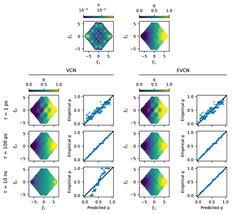
Figure 1: CV projections and reliability diagrams for AIB₉. (top left) CV projection of the stationary distribution. (top right) CV projection of the empirical committor. (left columns of VCN and EVCN) CV projections of the predicted committors. (right columns of VCN and EVCN) Reliability diagrams for the predicted committors. All results shown are obtained with the dihedral neural-network inputs.

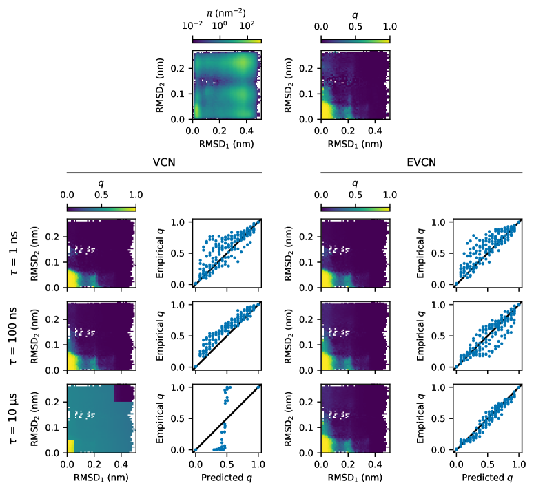
Figure 2: CV projections and reliability diagrams for Trp-cage. (top left) CV projection of the stationary distribution. (top right) CV projection of the empirical committor. (left columns of VCN and EVCN) CV projections of the predicted committors. (right columns of VCN and EVCN) Reliability diagrams for the predicted committors. All results shown are obtained with the dihedral neural-network inputs.

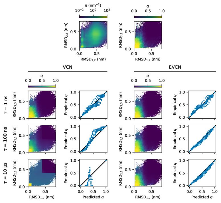
Figure 3: CV projections and reliability diagrams for villin. (top left) CV projection of the stationary distribution. (top right) CV projection of the empirical committor. (left columns of VCN and EVCN) CV projections of the predicted committors. (right columns of VCN and EVCN) Reliability diagrams for the predicted committors. All results shown are obtained with the dihedral neural-network inputs.

3.3 Committor

We examine the behavior of committors predicted using the VCN and EVCN loss functions at different lag times. We compute committors for individual conformations in the sampled trajectories and then visualize the results in two ways. First, we plot the average committor for structures in a bin defined by a pair of CV values. Second, we partition the predicted committor into 20 uniformly spaced bins over $[0,1]$, and for each bin, we plot the mean empirical committor against the mean predicted committor. In the latter set of plots, which we term “reliability diagrams” in line with the machine learning literature (which also calls them “calibration curves”), each point is from a single model. Perfect alignment between the predicted and empirical committors corresponds to points lying along the diagonal (shown in black).

We first look at AIB₉ (Fig. 1). At the shortest lag time (1), CV projections of the predicted committor exhibit a checkered pattern reflecting the boundaries of the intermediate states. The reliability diagrams show substantial noise, but the means follow the diagonal. These artifacts arise because the VCN and EVCN losses are both relatively insensitive to slowly decaying modes, encouraging the committor to be flat within intermediate states at the expense of transition states between them. At the intermediate lag time (100), the committor becomes qualitatively accurate for both loss functions. At the longest lag time (10), the committor for EVCN remains accurate, while the committor for VCN appears flattened in the transition region and exhibits large jumps near the boundaries of states $A$ and $B$. These behaviors are reflected in the reliability diagrams. We can explain this behavior by considering $\operatorname{\mathds{E}}[\hat{u}(X_{0})\hat{u}(X_{\tau})]\approx\operatorname{\mathds{E}}[\hat{u}(X_{0})]\operatorname{\mathds{E}}[\hat{u}(X_{\tau})]$ as $\tau\to\infty$. With this approximation, (22) is minimized when $u(x)=\mathds{1}_{B}(x)$ for $x\notin D$ and $u(x)=\operatorname{\mathds{E}}[\mathds{1}_{B}(X_{0})]/\operatorname{\mathds{E}}[\mathds{1}_{D^{\mathsf{c}}}(X_{0})]$ otherwise.

Next, we look at Trp-cage (Fig. 2). At the 1 lag time, both loss functions incorrectly predict the committor of the intermediate state above the folded basin in the CV projection to be near zero. Reflecting this, the reliability diagram has most points above the diagonal, where the empirical committor is greater than the predicted committor. At the 100 lag time, both methods resolve the intermediate state but the VCN predictions are lower (darker CV projection). Correspondingly, the reliability diagram for VCN has more points above the diagonal. For EVCN, on the other hand, the points are noisy but do not show obvious bias. With a 10 lag time, VCN breaks down. The CV projection shows that the predicted committor is flat in $D$, and the reliability diagram shows that all the predicted values (other than 0 in $A$ and 1 in $B$) are clustered near a single value. On the other hand, the CV projection of the EVCN result remains accurate, and the reliability diagram follows the diagonal with less noise than the 100 lag time.

Villin (Fig. 3) exhibits similar behavior to the previous systems. For the 1 lag time, both loss functions yield similar, good, predictions. However, at the 100 lag time, the EVCN prediction shows clear improvement over the VCN prediction, which is already beginning to flatten in the transition region. In the reliability diagrams, EVCN predictions are near the diagonal, while VCN predictions visibly deviate. At the 10 lag time, the VCN prediction is again clustered around a single value, while the EVCN prediction remains accurate.

			Transition rate hyperparameters
			VCN (22)			EVCN (19)
Committor hyperparameters			1	100	10	1	100	10
CVs	VCN	1	$7.0\text{\times}{10}^{-02}$	$1.3\text{\times}{10}^{-02}$	$6.8\text{\times}{10}^{-03}$	$7.0\text{\times}{10}^{-02}$	$1.3\text{\times}{10}^{-02}$	$9.1\text{\times}{10}^{-03}$
		100	$8.7\text{\times}{10}^{-02}$	$1.2\text{\times}{10}^{-02}$	$6.7\text{\times}{10}^{-03}$	$8.7\text{\times}{10}^{-02}$	$1.2\text{\times}{10}^{-02}$	$9.1\text{\times}{10}^{-03}$
		10	$8.2\text{\times}{10}^{00}$	$1.1\text{\times}{10}^{-01}$	$5.3\text{\times}{10}^{-03}$	$8.2\text{\times}{10}^{00}$	$1.8\text{\times}{10}^{-01}$	$1.1\text{\times}{10}^{-02}$
	EVCN	1	$7.0\text{\times}{10}^{-02}$	$1.3\text{\times}{10}^{-02}$	$6.8\text{\times}{10}^{-03}$	$7.0\text{\times}{10}^{-02}$	$1.3\text{\times}{10}^{-02}$	$9.1\text{\times}{10}^{-03}$
		100	$8.7\text{\times}{10}^{-02}$	$1.2\text{\times}{10}^{-02}$	$6.7\text{\times}{10}^{-03}$	$8.7\text{\times}{10}^{-02}$	$1.2\text{\times}{10}^{-02}$	$9.1\text{\times}{10}^{-03}$
		10	$9.8\text{\times}{10}^{-02}$	$1.2\text{\times}{10}^{-02}$	$6.7\text{\times}{10}^{-03}$	$9.8\text{\times}{10}^{-02}$	$1.2\text{\times}{10}^{-02}$	$9.1\text{\times}{10}^{-03}$
Dihedrals	VCN	1	$2.1\text{\times}{10}^{-02}$	$1.5\text{\times}{10}^{-02}$	$7.7\text{\times}{10}^{-03}$	$2.1\text{\times}{10}^{-02}$	$1.5\text{\times}{10}^{-02}$	$9.6\text{\times}{10}^{-03}$
		100	$2.8\text{\times}{10}^{-02}$	$9.9\text{\times}{10}^{-03}$	$6.7\text{\times}{10}^{-03}$	$2.8\text{\times}{10}^{-02}$	$1.0\text{\times}{10}^{-02}$	$9.1\text{\times}{10}^{-03}$
		10	$9.4\text{\times}{10}^{00}$	$1.2\text{\times}{10}^{-01}$	$5.3\text{\times}{10}^{-03}$	$9.4\text{\times}{10}^{00}$	$2.0\text{\times}{10}^{-01}$	$1.1\text{\times}{10}^{-02}$
	EVCN	1	$2.1\text{\times}{10}^{-02}$	$1.5\text{\times}{10}^{-02}$	$7.7\text{\times}{10}^{-03}$	$2.1\text{\times}{10}^{-02}$	$1.5\text{\times}{10}^{-02}$	$9.6\text{\times}{10}^{-03}$
		100	$2.7\text{\times}{10}^{-02}$	$9.9\text{\times}{10}^{-03}$	$6.7\text{\times}{10}^{-03}$	$2.7\text{\times}{10}^{-02}$	$9.9\text{\times}{10}^{-03}$	$9.1\text{\times}{10}^{-03}$
		10	$4.5\text{\times}{10}^{-02}$	$1.0\text{\times}{10}^{-02}$	$6.7\text{\times}{10}^{-03}$	$4.5\text{\times}{10}^{-02}$	$1.0\text{\times}{10}^{-02}$	$9.1\text{\times}{10}^{-03}$

Table 1: Predicted transition rates () for AIB₉, for different committor and transition rate estimator hyperparameters. The empirical transition rate if $9.1\times 10^{-3}$ .

			Transition rate hyperparameters
			VCN			EVCN
Committor hyperparameters			1	100	10	1	100	10
RMSDs	VCN	1	$6.7\text{\times}{10}^{-01}$	$8.3\text{\times}{10}^{-02}$	$1.4\text{\times}{10}^{-02}$	$6.9\text{\times}{10}^{-01}$	$1.2\text{\times}{10}^{-01}$	$7.7\text{\times}{10}^{-02}$
		100	$9.1\text{\times}{10}^{-01}$	$6.8\text{\times}{10}^{-02}$	$1.4\text{\times}{10}^{-02}$	$9.8\text{\times}{10}^{-01}$	$1.0\text{\times}{10}^{-01}$	$7.7\text{\times}{10}^{-02}$
		10	$1.8\text{\times}{10}^{01}$	$3.2\text{\times}{10}^{-01}$	$8.8\text{\times}{10}^{-03}$	$2.7\text{\times}{10}^{01}$	$7.7\text{\times}{10}^{-01}$	$8.6\text{\times}{10}^{-02}$
	EVCN	1	$6.8\text{\times}{10}^{-01}$	$8.4\text{\times}{10}^{-02}$	$1.4\text{\times}{10}^{-02}$	$6.9\text{\times}{10}^{-01}$	$1.2\text{\times}{10}^{-01}$	$7.7\text{\times}{10}^{-02}$
		100	$9.3\text{\times}{10}^{-01}$	$6.8\text{\times}{10}^{-02}$	$1.4\text{\times}{10}^{-02}$	$9.6\text{\times}{10}^{-01}$	$1.0\text{\times}{10}^{-01}$	$7.7\text{\times}{10}^{-02}$
		10	$9.6\text{\times}{10}^{-01}$	$7.2\text{\times}{10}^{-02}$	$1.4\text{\times}{10}^{-02}$	$9.9\text{\times}{10}^{-01}$	$1.0\text{\times}{10}^{-01}$	$7.7\text{\times}{10}^{-02}$
Dihedrals	VCN	1	$3.7\text{\times}{10}^{-01}$	$5.9\text{\times}{10}^{-02}$	$1.4\text{\times}{10}^{-02}$	$4.1\text{\times}{10}^{-01}$	$9.8\text{\times}{10}^{-02}$	$7.7\text{\times}{10}^{-02}$
		100	$5.1\text{\times}{10}^{-01}$	$5.4\text{\times}{10}^{-02}$	$1.4\text{\times}{10}^{-02}$	$6.3\text{\times}{10}^{-01}$	$8.9\text{\times}{10}^{-02}$	$7.7\text{\times}{10}^{-02}$
		10	$1.7\text{\times}{10}^{01}$	$3.4\text{\times}{10}^{-01}$	$8.9\text{\times}{10}^{-03}$	$2.7\text{\times}{10}^{01}$	$8.4\text{\times}{10}^{-01}$	$8.7\text{\times}{10}^{-02}$
	EVCN	1	$3.6\text{\times}{10}^{-01}$	$5.5\text{\times}{10}^{-02}$	$1.4\text{\times}{10}^{-02}$	$4.0\text{\times}{10}^{-01}$	$9.4\text{\times}{10}^{-02}$	$7.7\text{\times}{10}^{-02}$
		100	$5.0\text{\times}{10}^{-01}$	$5.5\text{\times}{10}^{-02}$	$1.5\text{\times}{10}^{-02}$	$5.3\text{\times}{10}^{-01}$	$8.5\text{\times}{10}^{-02}$	$7.7\text{\times}{10}^{-02}$
		10	$6.0\text{\times}{10}^{-01}$	$5.6\text{\times}{10}^{-02}$	$1.5\text{\times}{10}^{-02}$	$6.3\text{\times}{10}^{-01}$	$8.6\text{\times}{10}^{-02}$	$7.7\text{\times}{10}^{-02}$
Distances	VCN	1	$2.9\text{\times}{10}^{-01}$	$5.9\text{\times}{10}^{-02}$	$1.5\text{\times}{10}^{-02}$	$3.4\text{\times}{10}^{-01}$	$8.9\text{\times}{10}^{-02}$	$7.7\text{\times}{10}^{-02}$
		100	$4.5\text{\times}{10}^{-01}$	$5.0\text{\times}{10}^{-02}$	$1.4\text{\times}{10}^{-02}$	$5.9\text{\times}{10}^{-01}$	$8.8\text{\times}{10}^{-02}$	$7.7\text{\times}{10}^{-02}$
		10	$1.8\text{\times}{10}^{01}$	$3.3\text{\times}{10}^{-01}$	$8.8\text{\times}{10}^{-03}$	$2.7\text{\times}{10}^{01}$	$7.8\text{\times}{10}^{-01}$	$8.6\text{\times}{10}^{-02}$
	EVCN	1	$3.3\text{\times}{10}^{-01}$	$6.2\text{\times}{10}^{-02}$	$1.5\text{\times}{10}^{-02}$	$3.5\text{\times}{10}^{-01}$	$8.9\text{\times}{10}^{-02}$	$7.7\text{\times}{10}^{-02}$
		100	$4.4\text{\times}{10}^{-01}$	$5.3\text{\times}{10}^{-02}$	$1.5\text{\times}{10}^{-02}$	$4.9\text{\times}{10}^{-01}$	$8.5\text{\times}{10}^{-02}$	$7.7\text{\times}{10}^{-02}$
		10	$4.7\text{\times}{10}^{-01}$	$5.4\text{\times}{10}^{-02}$	$1.4\text{\times}{10}^{-02}$	$5.5\text{\times}{10}^{-01}$	$8.7\text{\times}{10}^{-02}$	$7.7\text{\times}{10}^{-02}$

Table 2: Predicted transition rates () for Trp-cage, for different committor and transition rate estimator hyperparameters. The empirical transition rate if $7.7\times 10^{-2}$ .

			Transition rate hyperparameters
			VCN			EVCN
Committor hyperparameters			1	100	10	1	100	10
RMSDs	VCN	1	$1.6\text{\times}{10}^{00}$	$3.1\text{\times}{10}^{-01}$	$1.6\text{\times}{10}^{-02}$	$1.6\text{\times}{10}^{00}$	$4.1\text{\times}{10}^{-01}$	$3.9\text{\times}{10}^{-01}$
		100	$2.7\text{\times}{10}^{00}$	$2.8\text{\times}{10}^{-01}$	$1.3\text{\times}{10}^{-02}$	$3.6\text{\times}{10}^{00}$	$4.6\text{\times}{10}^{-01}$	$3.9\text{\times}{10}^{-01}$
		10	$1.7\text{\times}{10}^{01}$	$4.0\text{\times}{10}^{-01}$	$9.4\text{\times}{10}^{-03}$	$2.6\text{\times}{10}^{01}$	$9.5\text{\times}{10}^{-01}$	$3.9\text{\times}{10}^{-01}$
	EVCN	1	$1.6\text{\times}{10}^{00}$	$3.1\text{\times}{10}^{-01}$	$1.6\text{\times}{10}^{-02}$	$1.6\text{\times}{10}^{00}$	$4.1\text{\times}{10}^{-01}$	$3.9\text{\times}{10}^{-01}$
		10	$1.9\text{\times}{10}^{00}$	$3.3\text{\times}{10}^{-01}$	$1.7\text{\times}{10}^{-02}$	$1.9\text{\times}{10}^{00}$	$4.0\text{\times}{10}^{-01}$	$3.9\text{\times}{10}^{-01}$
		100	$1.9\text{\times}{10}^{00}$	$3.3\text{\times}{10}^{-01}$	$1.7\text{\times}{10}^{-02}$	$1.9\text{\times}{10}^{00}$	$4.0\text{\times}{10}^{-01}$	$3.9\text{\times}{10}^{-01}$
Dihedrals	VCN	1	$1.1\text{\times}{10}^{00}$	$3.3\text{\times}{10}^{-01}$	$1.7\text{\times}{10}^{-02}$	$1.2\text{\times}{10}^{00}$	$3.9\text{\times}{10}^{-01}$	$3.9\text{\times}{10}^{-01}$
		100	$2.0\text{\times}{10}^{00}$	$2.9\text{\times}{10}^{-01}$	$1.4\text{\times}{10}^{-02}$	$2.5\text{\times}{10}^{00}$	$4.4\text{\times}{10}^{-01}$	$3.9\text{\times}{10}^{-01}$
		10	$1.8\text{\times}{10}^{01}$	$4.3\text{\times}{10}^{-01}$	$9.4\text{\times}{10}^{-03}$	$2.9\text{\times}{10}^{01}$	$1.0\text{\times}{10}^{00}$	$4.0\text{\times}{10}^{-01}$
	EVCN	1	$1.2\text{\times}{10}^{00}$	$3.3\text{\times}{10}^{-01}$	$1.7\text{\times}{10}^{-02}$	$1.2\text{\times}{10}^{00}$	$3.9\text{\times}{10}^{-01}$	$3.9\text{\times}{10}^{-01}$
		100	$1.9\text{\times}{10}^{00}$	$3.4\text{\times}{10}^{-01}$	$1.7\text{\times}{10}^{-02}$	$1.9\text{\times}{10}^{00}$	$4.0\text{\times}{10}^{-01}$	$3.9\text{\times}{10}^{-01}$
		10	$2.0\text{\times}{10}^{00}$	$3.4\text{\times}{10}^{-01}$	$1.7\text{\times}{10}^{-02}$	$2.1\text{\times}{10}^{00}$	$4.0\text{\times}{10}^{-01}$	$3.9\text{\times}{10}^{-01}$
Distances	VCN	1	$8.8\text{\times}{10}^{-01}$	$3.1\text{\times}{10}^{-01}$	$1.6\text{\times}{10}^{-02}$	$9.2\text{\times}{10}^{-01}$	$3.8\text{\times}{10}^{-01}$	$3.9\text{\times}{10}^{-01}$
		100	$1.8\text{\times}{10}^{00}$	$2.8\text{\times}{10}^{-01}$	$1.4\text{\times}{10}^{-02}$	$2.3\text{\times}{10}^{00}$	$4.4\text{\times}{10}^{-01}$	$3.9\text{\times}{10}^{-01}$
		10	$1.9\text{\times}{10}^{01}$	$4.3\text{\times}{10}^{-01}$	$9.4\text{\times}{10}^{-03}$	$3.0\text{\times}{10}^{01}$	$1.0\text{\times}{10}^{00}$	$4.0\text{\times}{10}^{-01}$
	EVCN	1	$9.0\text{\times}{10}^{-01}$	$3.1\text{\times}{10}^{-01}$	$1.7\text{\times}{10}^{-02}$	$9.3\text{\times}{10}^{-01}$	$3.8\text{\times}{10}^{-01}$	$3.9\text{\times}{10}^{-01}$
		100	$1.4\text{\times}{10}^{00}$	$3.2\text{\times}{10}^{-01}$	$1.7\text{\times}{10}^{-02}$	$1.4\text{\times}{10}^{00}$	$3.9\text{\times}{10}^{-01}$	$3.9\text{\times}{10}^{-01}$
		10	$1.5\text{\times}{10}^{00}$	$3.3\text{\times}{10}^{-01}$	$1.7\text{\times}{10}^{-02}$	$1.5\text{\times}{10}^{00}$	$3.9\text{\times}{10}^{-01}$	$3.9\text{\times}{10}^{-01}$

Table 3: Predicted transition rates () for villin, for different committor and transition rate estimator hyperparameters. The empirical transition rate if $3.7\times 10^{-1}$ .

			Transition rate hyperparameters
			(29) with VCN			(29) with EVCN
Committor hyperparameters			1, 100	1, 10	100, 10	1, 100	1, 10	100, 10
CVs	VCN	1	$1.2\text{\times}{10}^{-02}$	$6.8\text{\times}{10}^{-03}$	$6.7\text{\times}{10}^{-03}$	$1.2\text{\times}{10}^{-02}$	$9.1\text{\times}{10}^{-03}$	$9.1\text{\times}{10}^{-03}$
		100	$1.1\text{\times}{10}^{-02}$	$6.7\text{\times}{10}^{-03}$	$6.6\text{\times}{10}^{-03}$	$1.1\text{\times}{10}^{-02}$	$9.1\text{\times}{10}^{-03}$	$9.1\text{\times}{10}^{-03}$
		10	$2.4\text{\times}{10}^{-02}$	$4.5\text{\times}{10}^{-03}$	$4.3\text{\times}{10}^{-03}$	$9.7\text{\times}{10}^{-02}$	$1.0\text{\times}{10}^{-02}$	$9.4\text{\times}{10}^{-03}$
	EVCN	1	$1.2\text{\times}{10}^{-02}$	$6.8\text{\times}{10}^{-03}$	$6.7\text{\times}{10}^{-03}$	$1.2\text{\times}{10}^{-02}$	$9.1\text{\times}{10}^{-03}$	$9.1\text{\times}{10}^{-03}$
		100	$1.1\text{\times}{10}^{-02}$	$6.7\text{\times}{10}^{-03}$	$6.7\text{\times}{10}^{-03}$	$1.1\text{\times}{10}^{-02}$	$9.1\text{\times}{10}^{-03}$	$9.1\text{\times}{10}^{-03}$
		10	$1.1\text{\times}{10}^{-02}$	$6.7\text{\times}{10}^{-03}$	$6.6\text{\times}{10}^{-03}$	$1.1\text{\times}{10}^{-02}$	$9.1\text{\times}{10}^{-03}$	$9.1\text{\times}{10}^{-03}$
Dihedrals	VCN	1	$1.5\text{\times}{10}^{-02}$	$7.7\text{\times}{10}^{-03}$	$7.6\text{\times}{10}^{-03}$	$1.5\text{\times}{10}^{-02}$	$9.6\text{\times}{10}^{-03}$	$9.6\text{\times}{10}^{-03}$
		100	$9.7\text{\times}{10}^{-03}$	$6.7\text{\times}{10}^{-03}$	$6.6\text{\times}{10}^{-03}$	$9.8\text{\times}{10}^{-03}$	$9.1\text{\times}{10}^{-03}$	$9.1\text{\times}{10}^{-03}$
		10	$2.5\text{\times}{10}^{-02}$	$4.3\text{\times}{10}^{-03}$	$4.1\text{\times}{10}^{-03}$	$1.1\text{\times}{10}^{-01}$	$1.0\text{\times}{10}^{-02}$	$9.4\text{\times}{10}^{-03}$
	EVCN	1	$1.5\text{\times}{10}^{-02}$	$7.7\text{\times}{10}^{-03}$	$7.6\text{\times}{10}^{-03}$	$1.5\text{\times}{10}^{-02}$	$9.6\text{\times}{10}^{-03}$	$9.6\text{\times}{10}^{-03}$
		100	$9.7\text{\times}{10}^{-03}$	$6.7\text{\times}{10}^{-03}$	$6.7\text{\times}{10}^{-03}$	$9.8\text{\times}{10}^{-03}$	$9.1\text{\times}{10}^{-03}$	$9.1\text{\times}{10}^{-03}$
		10	$9.9\text{\times}{10}^{-03}$	$6.7\text{\times}{10}^{-03}$	$6.6\text{\times}{10}^{-03}$	$1.0\text{\times}{10}^{-02}$	$9.1\text{\times}{10}^{-03}$	$9.1\text{\times}{10}^{-03}$

Table 4: Transition rates () predicted using (29) for AIB₉, for different committor and transition rate estimator hyperparameters. The empirical transition rate if $9.1\times 10^{-3}$ .

			Transition rate hyperparameters
			(29) with VCN			(29) with EVCN
Committor hyperparameters			1, 100	1, 10	100, 10	1, 100	1, 10	100, 10
RMSDs	VCN	1	$7.7\text{\times}{10}^{-02}$	$1.4\text{\times}{10}^{-02}$	$1.3\text{\times}{10}^{-02}$	$1.1\text{\times}{10}^{-01}$	$7.7\text{\times}{10}^{-02}$	$7.7\text{\times}{10}^{-02}$
		100	$5.9\text{\times}{10}^{-02}$	$1.4\text{\times}{10}^{-02}$	$1.3\text{\times}{10}^{-02}$	$9.5\text{\times}{10}^{-02}$	$7.7\text{\times}{10}^{-02}$	$7.7\text{\times}{10}^{-02}$
		10	$1.5\text{\times}{10}^{-01}$	$7.1\text{\times}{10}^{-03}$	$5.6\text{\times}{10}^{-03}$	$5.1\text{\times}{10}^{-01}$	$8.3\text{\times}{10}^{-02}$	$7.9\text{\times}{10}^{-02}$
	EVCN	1	$7.8\text{\times}{10}^{-02}$	$1.4\text{\times}{10}^{-02}$	$1.3\text{\times}{10}^{-02}$	$1.1\text{\times}{10}^{-01}$	$7.7\text{\times}{10}^{-02}$	$7.7\text{\times}{10}^{-02}$
		100	$5.9\text{\times}{10}^{-02}$	$1.4\text{\times}{10}^{-02}$	$1.4\text{\times}{10}^{-02}$	$9.2\text{\times}{10}^{-02}$	$7.7\text{\times}{10}^{-02}$	$7.7\text{\times}{10}^{-02}$
		10	$6.3\text{\times}{10}^{-02}$	$1.4\text{\times}{10}^{-02}$	$1.4\text{\times}{10}^{-02}$	$9.4\text{\times}{10}^{-02}$	$7.7\text{\times}{10}^{-02}$	$7.7\text{\times}{10}^{-02}$
Dihedrals	VCN	1	$5.6\text{\times}{10}^{-02}$	$1.4\text{\times}{10}^{-02}$	$1.4\text{\times}{10}^{-02}$	$9.5\text{\times}{10}^{-02}$	$7.7\text{\times}{10}^{-02}$	$7.7\text{\times}{10}^{-02}$
		100	$4.9\text{\times}{10}^{-02}$	$1.4\text{\times}{10}^{-02}$	$1.4\text{\times}{10}^{-02}$	$8.4\text{\times}{10}^{-02}$	$7.7\text{\times}{10}^{-02}$	$7.7\text{\times}{10}^{-02}$
		10	$1.7\text{\times}{10}^{-01}$	$7.2\text{\times}{10}^{-03}$	$5.6\text{\times}{10}^{-03}$	$5.7\text{\times}{10}^{-01}$	$8.4\text{\times}{10}^{-02}$	$7.9\text{\times}{10}^{-02}$
	EVCN	1	$5.2\text{\times}{10}^{-02}$	$1.4\text{\times}{10}^{-02}$	$1.4\text{\times}{10}^{-02}$	$9.1\text{\times}{10}^{-02}$	$7.7\text{\times}{10}^{-02}$	$7.7\text{\times}{10}^{-02}$
		100	$5.0\text{\times}{10}^{-02}$	$1.5\text{\times}{10}^{-02}$	$1.4\text{\times}{10}^{-02}$	$8.0\text{\times}{10}^{-02}$	$7.7\text{\times}{10}^{-02}$	$7.7\text{\times}{10}^{-02}$
		10	$5.1\text{\times}{10}^{-02}$	$1.4\text{\times}{10}^{-02}$	$1.4\text{\times}{10}^{-02}$	$8.0\text{\times}{10}^{-02}$	$7.7\text{\times}{10}^{-02}$	$7.7\text{\times}{10}^{-02}$
Distances	VCN	1	$5.7\text{\times}{10}^{-02}$	$1.5\text{\times}{10}^{-02}$	$1.4\text{\times}{10}^{-02}$	$8.6\text{\times}{10}^{-02}$	$7.7\text{\times}{10}^{-02}$	$7.7\text{\times}{10}^{-02}$
		100	$4.6\text{\times}{10}^{-02}$	$1.4\text{\times}{10}^{-02}$	$1.4\text{\times}{10}^{-02}$	$8.3\text{\times}{10}^{-02}$	$7.7\text{\times}{10}^{-02}$	$7.7\text{\times}{10}^{-02}$
		10	$1.5\text{\times}{10}^{-01}$	$7.1\text{\times}{10}^{-03}$	$5.6\text{\times}{10}^{-03}$	$5.1\text{\times}{10}^{-01}$	$8.3\text{\times}{10}^{-02}$	$7.9\text{\times}{10}^{-02}$
	EVCN	1	$5.9\text{\times}{10}^{-02}$	$1.5\text{\times}{10}^{-02}$	$1.4\text{\times}{10}^{-02}$	$8.6\text{\times}{10}^{-02}$	$7.7\text{\times}{10}^{-02}$	$7.7\text{\times}{10}^{-02}$
		100	$4.9\text{\times}{10}^{-02}$	$1.4\text{\times}{10}^{-02}$	$1.4\text{\times}{10}^{-02}$	$8.1\text{\times}{10}^{-02}$	$7.7\text{\times}{10}^{-02}$	$7.7\text{\times}{10}^{-02}$
		10	$4.9\text{\times}{10}^{-02}$	$1.4\text{\times}{10}^{-02}$	$1.4\text{\times}{10}^{-02}$	$8.3\text{\times}{10}^{-02}$	$7.7\text{\times}{10}^{-02}$	$7.7\text{\times}{10}^{-02}$

Table 5: Transition rates () predicted using (29) for Trp-cage, for different committor and transition rate estimator hyperparameters. The empirical transition rate if $7.7\times 10^{-2}$ .

			Transition rate hyperparameters
			(29) with VCN			(29) with EVCN
Committor hyperparameters			1, 100	1, 10	100, 10	1, 100	1, 10	100, 10
RMSDs	VCN	1	$2.9\text{\times}{10}^{-01}$	$1.5\text{\times}{10}^{-02}$	$1.3\text{\times}{10}^{-02}$	$4.0\text{\times}{10}^{-01}$	$3.9\text{\times}{10}^{-01}$	$3.9\text{\times}{10}^{-01}$
		100	$2.5\text{\times}{10}^{-01}$	$1.3\text{\times}{10}^{-02}$	$1.0\text{\times}{10}^{-02}$	$4.3\text{\times}{10}^{-01}$	$3.9\text{\times}{10}^{-01}$	$3.9\text{\times}{10}^{-01}$
		10	$2.4\text{\times}{10}^{-01}$	$7.8\text{\times}{10}^{-03}$	$5.5\text{\times}{10}^{-03}$	$7.0\text{\times}{10}^{-01}$	$3.9\text{\times}{10}^{-01}$	$3.9\text{\times}{10}^{-01}$
	EVCN	1	$3.0\text{\times}{10}^{-01}$	$1.6\text{\times}{10}^{-02}$	$1.3\text{\times}{10}^{-02}$	$4.0\text{\times}{10}^{-01}$	$3.9\text{\times}{10}^{-01}$	$3.9\text{\times}{10}^{-01}$
		100	$3.2\text{\times}{10}^{-01}$	$1.7\text{\times}{10}^{-02}$	$1.4\text{\times}{10}^{-02}$	$3.9\text{\times}{10}^{-01}$	$3.9\text{\times}{10}^{-01}$	$3.9\text{\times}{10}^{-01}$
		10	$3.1\text{\times}{10}^{-01}$	$1.6\text{\times}{10}^{-02}$	$1.3\text{\times}{10}^{-02}$	$3.9\text{\times}{10}^{-01}$	$3.9\text{\times}{10}^{-01}$	$3.9\text{\times}{10}^{-01}$
Dihedrals	VCN	1	$3.2\text{\times}{10}^{-01}$	$1.7\text{\times}{10}^{-02}$	$1.4\text{\times}{10}^{-02}$	$3.9\text{\times}{10}^{-01}$	$3.9\text{\times}{10}^{-01}$	$3.9\text{\times}{10}^{-01}$
		100	$2.7\text{\times}{10}^{-01}$	$1.4\text{\times}{10}^{-02}$	$1.2\text{\times}{10}^{-02}$	$4.2\text{\times}{10}^{-01}$	$3.9\text{\times}{10}^{-01}$	$3.9\text{\times}{10}^{-01}$
		10	$2.5\text{\times}{10}^{-01}$	$7.6\text{\times}{10}^{-03}$	$5.2\text{\times}{10}^{-03}$	$7.5\text{\times}{10}^{-01}$	$3.9\text{\times}{10}^{-01}$	$3.9\text{\times}{10}^{-01}$
	EVCN	1	$3.2\text{\times}{10}^{-01}$	$1.7\text{\times}{10}^{-02}$	$1.4\text{\times}{10}^{-02}$	$3.8\text{\times}{10}^{-01}$	$3.9\text{\times}{10}^{-01}$	$3.9\text{\times}{10}^{-01}$
		100	$3.2\text{\times}{10}^{-01}$	$1.7\text{\times}{10}^{-02}$	$1.4\text{\times}{10}^{-02}$	$3.9\text{\times}{10}^{-01}$	$3.9\text{\times}{10}^{-01}$	$3.9\text{\times}{10}^{-01}$
		10	$3.2\text{\times}{10}^{-01}$	$1.7\text{\times}{10}^{-02}$	$1.4\text{\times}{10}^{-02}$	$3.9\text{\times}{10}^{-01}$	$3.9\text{\times}{10}^{-01}$	$3.9\text{\times}{10}^{-01}$
Distances	VCN	1	$3.0\text{\times}{10}^{-01}$	$1.6\text{\times}{10}^{-02}$	$1.3\text{\times}{10}^{-02}$	$3.8\text{\times}{10}^{-01}$	$3.9\text{\times}{10}^{-01}$	$3.9\text{\times}{10}^{-01}$
		100	$2.6\text{\times}{10}^{-01}$	$1.4\text{\times}{10}^{-02}$	$1.1\text{\times}{10}^{-02}$	$4.2\text{\times}{10}^{-01}$	$3.9\text{\times}{10}^{-01}$	$3.9\text{\times}{10}^{-01}$
		10	$2.5\text{\times}{10}^{-01}$	$7.5\text{\times}{10}^{-03}$	$5.1\text{\times}{10}^{-03}$	$7.4\text{\times}{10}^{-01}$	$3.9\text{\times}{10}^{-01}$	$3.9\text{\times}{10}^{-01}$
	EVCN	1	$3.0\text{\times}{10}^{-01}$	$1.7\text{\times}{10}^{-02}$	$1.4\text{\times}{10}^{-02}$	$3.8\text{\times}{10}^{-01}$	$3.9\text{\times}{10}^{-01}$	$3.9\text{\times}{10}^{-01}$
		100	$3.1\text{\times}{10}^{-01}$	$1.7\text{\times}{10}^{-02}$	$1.4\text{\times}{10}^{-02}$	$3.8\text{\times}{10}^{-01}$	$3.9\text{\times}{10}^{-01}$	$3.9\text{\times}{10}^{-01}$
		10	$3.2\text{\times}{10}^{-01}$	$1.7\text{\times}{10}^{-02}$	$1.4\text{\times}{10}^{-02}$	$3.8\text{\times}{10}^{-01}$	$3.9\text{\times}{10}^{-01}$	$3.9\text{\times}{10}^{-01}$

Table 6: Transition rates () predicted using (29) for villin, for different committor and transition rate estimator hyperparameters. The empirical transition rate if $3.7\times 10^{-1}$ .

3.4 Transition rate

In Tables 1, 2, and 3, we examine the transition rates predicted by the VCN and EVCN loss functions with various lag times. The loss function and lag time can affect the transition rates through both training the neural network for the committor and application of the rate formula given the trained committor. To distinguish these effects, we evaluate the rates using loss functions and lag times (columns) that are independent of those used to obtain the committors (rows). Unsurprisingly, more accurate committors yield more accurate transition rates. Still, even for a given committor (row), the loss function and lag time used to predict the rate (column) noticeably affect the result. As in the previous section, rates are overestimated at short lag times and approach their correct values as lag times increase. At long lag times, the VCN loss predicts rates that go to zero (approximately proportional to $1/\tau$, as can be seen by substituting a constant committor value for $x\in D$, consistent with the flattening observed above), whereas the EVCN loss predicts rates that plateau near the true value. The choice of input features has a larger impact at shorter lag times. Less expressive input features—such as the CVs for AIB₉ and the RMSDs for Trp-cage and villin—tend to produce larger overestimates of the transition rate.

We examine the estimator in (29) in Tables 4, 5, and 6. We observe that using (29) with EVCN consistently yields more accurate rate estimates than (19) by itself. Rates predicted using the VCN loss (22) or its counterpart with (29) are not variational and tend to underestimate the rate at all but the shortest lag times. For both VCN and EVCN, the choice of the longer of the two lag times in (29) appears to matter more than the choice of the shorter of the two lag times.

			Mean squared error hyperparameters
			(28)	(30) with VCN			(30) with EVCN
Committor hyperparameters				1, 100	1, 10	100, 10	1, 100	1, 10	100, 10
CVs	VCN	1	$1.6\text{\times}{10}^{-05}$	$5.8\text{\times}{10}^{-05}$	$6.3\text{\times}{10}^{-05}$	$5.8\text{\times}{10}^{-04}$	$5.8\text{\times}{10}^{-05}$	$6.1\text{\times}{10}^{-05}$	$3.5\text{\times}{10}^{-04}$
		100	$-5.0\text{\times}{10}^{-04}$	$7.6\text{\times}{10}^{-05}$	$8.0\text{\times}{10}^{-05}$	$5.0\text{\times}{10}^{-04}$	$7.6\text{\times}{10}^{-05}$	$7.8\text{\times}{10}^{-05}$	$2.7\text{\times}{10}^{-04}$
		10	$1.9\text{\times}{10}^{-02}$	$8.2\text{\times}{10}^{-03}$	$8.2\text{\times}{10}^{-03}$	$1.0\text{\times}{10}^{-02}$	$8.1\text{\times}{10}^{-03}$	$8.2\text{\times}{10}^{-03}$	$1.7\text{\times}{10}^{-02}$
	EVCN	1	$1.6\text{\times}{10}^{-05}$	$5.8\text{\times}{10}^{-05}$	$6.3\text{\times}{10}^{-05}$	$5.8\text{\times}{10}^{-04}$	$5.8\text{\times}{10}^{-05}$	$6.1\text{\times}{10}^{-05}$	$3.5\text{\times}{10}^{-04}$
		100	$-4.9\text{\times}{10}^{-04}$	$7.7\text{\times}{10}^{-05}$	$8.1\text{\times}{10}^{-05}$	$5.0\text{\times}{10}^{-04}$	$7.7\text{\times}{10}^{-05}$	$7.8\text{\times}{10}^{-05}$	$2.7\text{\times}{10}^{-04}$
		10	$-5.0\text{\times}{10}^{-04}$	$8.7\text{\times}{10}^{-05}$	$9.2\text{\times}{10}^{-05}$	$5.2\text{\times}{10}^{-04}$	$8.7\text{\times}{10}^{-05}$	$8.9\text{\times}{10}^{-05}$	$2.9\text{\times}{10}^{-04}$
Dihedrals	VCN	1	$4.9\text{\times}{10}^{-03}$	$6.4\text{\times}{10}^{-06}$	$1.3\text{\times}{10}^{-05}$	$7.1\text{\times}{10}^{-04}$	$6.4\text{\times}{10}^{-06}$	$1.2\text{\times}{10}^{-05}$	$5.2\text{\times}{10}^{-04}$
		100	$-6.8\text{\times}{10}^{-04}$	$1.8\text{\times}{10}^{-05}$	$2.1\text{\times}{10}^{-05}$	$3.2\text{\times}{10}^{-04}$	$1.8\text{\times}{10}^{-05}$	$1.9\text{\times}{10}^{-05}$	$9.0\text{\times}{10}^{-05}$
		10	$2.2\text{\times}{10}^{-02}$	$9.3\text{\times}{10}^{-03}$	$9.3\text{\times}{10}^{-03}$	$1.1\text{\times}{10}^{-02}$	$9.2\text{\times}{10}^{-03}$	$9.3\text{\times}{10}^{-03}$	$1.9\text{\times}{10}^{-02}$
	EVCN	1	$4.9\text{\times}{10}^{-03}$	$6.4\text{\times}{10}^{-06}$	$1.3\text{\times}{10}^{-05}$	$7.1\text{\times}{10}^{-04}$	$6.4\text{\times}{10}^{-06}$	$1.2\text{\times}{10}^{-05}$	$5.2\text{\times}{10}^{-04}$
		100	$-6.7\text{\times}{10}^{-04}$	$1.7\text{\times}{10}^{-05}$	$2.0\text{\times}{10}^{-05}$	$3.2\text{\times}{10}^{-04}$	$1.7\text{\times}{10}^{-05}$	$1.8\text{\times}{10}^{-05}$	$8.8\text{\times}{10}^{-05}$
		10	$-7.1\text{\times}{10}^{-04}$	$3.5\text{\times}{10}^{-05}$	$3.9\text{\times}{10}^{-05}$	$3.6\text{\times}{10}^{-04}$	$3.5\text{\times}{10}^{-05}$	$3.6\text{\times}{10}^{-05}$	$1.3\text{\times}{10}^{-04}$

Table 7: Mean squared error in the predicted committor for AIB₉, for different committor and MSE estimator hyperparameters.

			Mean squared error hyperparameters
			(28)	(30) with VCN			(30) with EVCN
Committor hyperparameters				1, 100	1, 10	100, 10	1, 100	1, 10	100, 10
RMSDs	VCN	1	$4.8\text{\times}{10}^{-03}$	$6.0\text{\times}{10}^{-04}$	$6.6\text{\times}{10}^{-04}$	$7.0\text{\times}{10}^{-03}$	$5.8\text{\times}{10}^{-04}$	$6.1\text{\times}{10}^{-04}$	$3.9\text{\times}{10}^{-03}$
		100	$3.3\text{\times}{10}^{-03}$	$8.6\text{\times}{10}^{-04}$	$9.0\text{\times}{10}^{-04}$	$5.4\text{\times}{10}^{-03}$	$8.8\text{\times}{10}^{-04}$	$9.0\text{\times}{10}^{-04}$	$2.7\text{\times}{10}^{-03}$
		10	$9.0\text{\times}{10}^{-02}$	$1.7\text{\times}{10}^{-02}$	$1.8\text{\times}{10}^{-02}$	$3.2\text{\times}{10}^{-02}$	$2.7\text{\times}{10}^{-02}$	$2.7\text{\times}{10}^{-02}$	$6.9\text{\times}{10}^{-02}$
	EVCN	1	$4.8\text{\times}{10}^{-03}$	$6.0\text{\times}{10}^{-04}$	$6.6\text{\times}{10}^{-04}$	$7.1\text{\times}{10}^{-03}$	$5.8\text{\times}{10}^{-04}$	$6.1\text{\times}{10}^{-04}$	$3.9\text{\times}{10}^{-03}$
		100	$2.7\text{\times}{10}^{-03}$	$8.7\text{\times}{10}^{-04}$	$9.1\text{\times}{10}^{-04}$	$5.4\text{\times}{10}^{-03}$	$8.6\text{\times}{10}^{-04}$	$8.8\text{\times}{10}^{-04}$	$2.4\text{\times}{10}^{-03}$
		10	$2.8\text{\times}{10}^{-03}$	$9.0\text{\times}{10}^{-04}$	$9.5\text{\times}{10}^{-04}$	$5.8\text{\times}{10}^{-03}$	$8.9\text{\times}{10}^{-04}$	$9.1\text{\times}{10}^{-04}$	$2.7\text{\times}{10}^{-03}$
Dihedrals	VCN	1	$3.4\text{\times}{10}^{-03}$	$3.1\text{\times}{10}^{-04}$	$3.6\text{\times}{10}^{-04}$	$4.5\text{\times}{10}^{-03}$	$3.1\text{\times}{10}^{-04}$	$3.3\text{\times}{10}^{-04}$	$2.2\text{\times}{10}^{-03}$
		100	$1.1\text{\times}{10}^{-03}$	$4.6\text{\times}{10}^{-04}$	$4.9\text{\times}{10}^{-04}$	$4.0\text{\times}{10}^{-03}$	$5.5\text{\times}{10}^{-04}$	$5.5\text{\times}{10}^{-04}$	$1.2\text{\times}{10}^{-03}$
		10	$1.0\text{\times}{10}^{-01}$	$1.7\text{\times}{10}^{-02}$	$1.7\text{\times}{10}^{-02}$	$3.3\text{\times}{10}^{-02}$	$2.6\text{\times}{10}^{-02}$	$2.7\text{\times}{10}^{-02}$	$7.6\text{\times}{10}^{-02}$
	EVCN	1	$2.9\text{\times}{10}^{-03}$	$3.1\text{\times}{10}^{-04}$	$3.5\text{\times}{10}^{-04}$	$4.1\text{\times}{10}^{-03}$	$3.1\text{\times}{10}^{-04}$	$3.2\text{\times}{10}^{-04}$	$1.8\text{\times}{10}^{-03}$
		100	$6.5\text{\times}{10}^{-04}$	$4.5\text{\times}{10}^{-04}$	$4.9\text{\times}{10}^{-04}$	$4.1\text{\times}{10}^{-03}$	$4.5\text{\times}{10}^{-04}$	$4.6\text{\times}{10}^{-04}$	$8.2\text{\times}{10}^{-04}$
		10	$7.7\text{\times}{10}^{-04}$	$5.5\text{\times}{10}^{-04}$	$5.9\text{\times}{10}^{-04}$	$4.2\text{\times}{10}^{-03}$	$5.5\text{\times}{10}^{-04}$	$5.6\text{\times}{10}^{-04}$	$9.3\text{\times}{10}^{-04}$
Distances	VCN	1	$1.2\text{\times}{10}^{-03}$	$2.3\text{\times}{10}^{-04}$	$2.7\text{\times}{10}^{-04}$	$4.5\text{\times}{10}^{-03}$	$2.5\text{\times}{10}^{-04}$	$2.6\text{\times}{10}^{-04}$	$1.2\text{\times}{10}^{-03}$
		100	$1.2\text{\times}{10}^{-03}$	$4.1\text{\times}{10}^{-04}$	$4.4\text{\times}{10}^{-04}$	$3.6\text{\times}{10}^{-03}$	$5.0\text{\times}{10}^{-04}$	$5.1\text{\times}{10}^{-04}$	$1.1\text{\times}{10}^{-03}$
		10	$9.2\text{\times}{10}^{-02}$	$1.8\text{\times}{10}^{-02}$	$1.8\text{\times}{10}^{-02}$	$3.2\text{\times}{10}^{-02}$	$2.7\text{\times}{10}^{-02}$	$2.7\text{\times}{10}^{-02}$	$7.0\text{\times}{10}^{-02}$
	EVCN	1	$1.1\text{\times}{10}^{-03}$	$2.7\text{\times}{10}^{-04}$	$3.1\text{\times}{10}^{-04}$	$4.7\text{\times}{10}^{-03}$	$2.6\text{\times}{10}^{-04}$	$2.7\text{\times}{10}^{-04}$	$1.2\text{\times}{10}^{-03}$
		100	$6.6\text{\times}{10}^{-04}$	$3.9\text{\times}{10}^{-04}$	$4.2\text{\times}{10}^{-04}$	$3.9\text{\times}{10}^{-03}$	$4.0\text{\times}{10}^{-04}$	$4.1\text{\times}{10}^{-04}$	$8.9\text{\times}{10}^{-04}$
		10	$9.3\text{\times}{10}^{-04}$	$4.2\text{\times}{10}^{-04}$	$4.5\text{\times}{10}^{-04}$	$4.0\text{\times}{10}^{-03}$	$4.6\text{\times}{10}^{-04}$	$4.7\text{\times}{10}^{-04}$	$1.1\text{\times}{10}^{-03}$

Table 8: Mean squared error in the predicted committor for Trp-cage, for different committor and MSE estimator hyperparameters.

			Mean squared error hyperparameters
			(28)	(30) with VCN			(30) with EVCN
Committor hyperparameters				1, 100	1, 10	100, 10	1, 100	1, 10	100, 10
RMSDs	VCN	1	$4.3\text{\times}{10}^{-03}$	$1.3\text{\times}{10}^{-03}$	$1.5\text{\times}{10}^{-03}$	$2.9\text{\times}{10}^{-02}$	$1.2\text{\times}{10}^{-03}$	$1.2\text{\times}{10}^{-03}$	$2.3\text{\times}{10}^{-03}$
		100	$9.7\text{\times}{10}^{-03}$	$2.4\text{\times}{10}^{-03}$	$2.7\text{\times}{10}^{-03}$	$2.7\text{\times}{10}^{-02}$	$3.2\text{\times}{10}^{-03}$	$3.2\text{\times}{10}^{-03}$	$7.6\text{\times}{10}^{-03}$
		10	$5.9\text{\times}{10}^{-02}$	$1.6\text{\times}{10}^{-02}$	$1.7\text{\times}{10}^{-02}$	$4.0\text{\times}{10}^{-02}$	$2.6\text{\times}{10}^{-02}$	$2.6\text{\times}{10}^{-02}$	$5.7\text{\times}{10}^{-02}$
	EVCN	1	$4.1\text{\times}{10}^{-03}$	$1.3\text{\times}{10}^{-03}$	$1.6\text{\times}{10}^{-03}$	$3.0\text{\times}{10}^{-02}$	$1.2\text{\times}{10}^{-03}$	$1.2\text{\times}{10}^{-03}$	$2.0\text{\times}{10}^{-03}$
		100	$3.6\text{\times}{10}^{-03}$	$1.5\text{\times}{10}^{-03}$	$1.8\text{\times}{10}^{-03}$	$3.2\text{\times}{10}^{-02}$	$1.5\text{\times}{10}^{-03}$	$1.5\text{\times}{10}^{-03}$	$1.5\text{\times}{10}^{-03}$
		10	$3.6\text{\times}{10}^{-03}$	$1.6\text{\times}{10}^{-03}$	$1.9\text{\times}{10}^{-03}$	$3.2\text{\times}{10}^{-02}$	$1.5\text{\times}{10}^{-03}$	$1.5\text{\times}{10}^{-03}$	$1.5\text{\times}{10}^{-03}$
Dihedrals	VCN	1	$2.5\text{\times}{10}^{-03}$	$7.9\text{\times}{10}^{-04}$	$1.1\text{\times}{10}^{-03}$	$3.2\text{\times}{10}^{-02}$	$7.8\text{\times}{10}^{-04}$	$7.7\text{\times}{10}^{-04}$	$5.4\text{\times}{10}^{-04}$
		100	$7.6\text{\times}{10}^{-03}$	$1.7\text{\times}{10}^{-03}$	$1.9\text{\times}{10}^{-03}$	$2.8\text{\times}{10}^{-02}$	$2.1\text{\times}{10}^{-03}$	$2.1\text{\times}{10}^{-03}$	$5.6\text{\times}{10}^{-03}$
		10	$6.7\text{\times}{10}^{-02}$	$1.8\text{\times}{10}^{-02}$	$1.8\text{\times}{10}^{-02}$	$4.2\text{\times}{10}^{-02}$	$2.8\text{\times}{10}^{-02}$	$2.8\text{\times}{10}^{-02}$	$6.4\text{\times}{10}^{-02}$
	EVCN	1	$2.3\text{\times}{10}^{-03}$	$8.5\text{\times}{10}^{-04}$	$1.2\text{\times}{10}^{-03}$	$3.2\text{\times}{10}^{-02}$	$8.2\text{\times}{10}^{-04}$	$8.1\text{\times}{10}^{-04}$	$4.4\text{\times}{10}^{-04}$
		100	$3.3\text{\times}{10}^{-03}$	$1.6\text{\times}{10}^{-03}$	$1.9\text{\times}{10}^{-03}$	$3.2\text{\times}{10}^{-02}$	$1.5\text{\times}{10}^{-03}$	$1.5\text{\times}{10}^{-03}$	$1.4\text{\times}{10}^{-03}$
		10	$3.5\text{\times}{10}^{-03}$	$1.7\text{\times}{10}^{-03}$	$2.0\text{\times}{10}^{-03}$	$3.3\text{\times}{10}^{-02}$	$1.7\text{\times}{10}^{-03}$	$1.7\text{\times}{10}^{-03}$	$1.6\text{\times}{10}^{-03}$
Distances	VCN	1	$1.4\text{\times}{10}^{-03}$	$5.8\text{\times}{10}^{-04}$	$8.7\text{\times}{10}^{-04}$	$2.9\text{\times}{10}^{-02}$	$5.4\text{\times}{10}^{-04}$	$5.3\text{\times}{10}^{-04}$	$-5.3\text{\times}{10}^{-04}$
		100	$6.8\text{\times}{10}^{-03}$	$1.5\text{\times}{10}^{-03}$	$1.7\text{\times}{10}^{-03}$	$2.7\text{\times}{10}^{-02}$	$1.9\text{\times}{10}^{-03}$	$2.0\text{\times}{10}^{-03}$	$4.8\text{\times}{10}^{-03}$
		10	$6.7\text{\times}{10}^{-02}$	$1.9\text{\times}{10}^{-02}$	$1.9\text{\times}{10}^{-02}$	$4.3\text{\times}{10}^{-02}$	$2.9\text{\times}{10}^{-02}$	$3.0\text{\times}{10}^{-02}$	$6.4\text{\times}{10}^{-02}$
	EVCN	1	$1.3\text{\times}{10}^{-03}$	$6.0\text{\times}{10}^{-04}$	$8.9\text{\times}{10}^{-04}$	$3.0\text{\times}{10}^{-02}$	$5.5\text{\times}{10}^{-04}$	$5.4\text{\times}{10}^{-04}$	$-6.2\text{\times}{10}^{-04}$
		100	$2.4\text{\times}{10}^{-03}$	$1.0\text{\times}{10}^{-03}$	$1.3\text{\times}{10}^{-03}$	$3.1\text{\times}{10}^{-02}$	$1.0\text{\times}{10}^{-03}$	$1.0\text{\times}{10}^{-03}$	$4.6\text{\times}{10}^{-04}$
		10	$2.4\text{\times}{10}^{-03}$	$1.1\text{\times}{10}^{-03}$	$1.4\text{\times}{10}^{-03}$	$3.1\text{\times}{10}^{-02}$	$1.1\text{\times}{10}^{-03}$	$1.1\text{\times}{10}^{-03}$	$4.3\text{\times}{10}^{-04}$

Table 9: Mean squared error in the predicted committor for villin, for different committor and MSE estimator hyperparameters.

3.5 Mean squared error

In Tables 7, 8, and 9, we show MSE estimates (mean of 10 models) for the predicted committor under various training hyperparameters. Focusing first on the column computed with (28), at short lag times, committors trained with the VCN and EVCN loss function have similar errors. Notably, more expressive features do not always yield lower error. For EVCN, increasing the lag time tends to reduce the MSE until it plateaus, potentially above zero if the input features fail to capture all relevant degrees of freedom. In contrast, for VCN, the MSE initially decreases with lag time, but then increases as the approximation breaks down.

In Tables 7, 8, and 9, we also compare (30) with (28). The two estimators generally track each other, but (30) can differ from (28) by an order of magnitude when using VCN with long lag times. For villin, the approximation becomes negative for ECVN at long lag times, likely due to statistical noise. In contrast to (29), for a given committor (row), the choice of the shorter of the two lag times appears to have more impact on the MSE approximated by (30) than the choice of the longer of the two lag times.

4 Discussion

In this work, we derived an exact multiple-time-step expression for the transition rate and demonstrated, using models of molecular systems, that a variational scheme based on this expression yields accurate committors and transition rates with relatively little sensitivity to the choice of lag time. Our approach extends previous methods ¹⁸, which are valid only in the limit of a single-time-step lag time and break down at longer lag times.

We suggest several directions for improvement. For datasets composed of short trajectories, long lag times are inaccessible and so the method may struggle to capture slow modes. This may be addressed by using loss functions with greater sensitivity to these modes, such as (29). More advanced approaches incorporating memory, such as those proposed for slow modes in Ref. 48, may further improve accuracy.

Overfitting is also a challenge, and standard regularization techniques are often ineffective. We expect that integrating over lag times, as in Ref. 49, may reduce overfitting and improve robustness. We are exploring regularization strategies that directly restrain the committor to depend on physical or learned CVs in a simple way.

Finally, the variational methods considered in the present study assume detailed balance and equilibrium sampling (or equilibrium reweighting). Theoretical ⁵⁰ and empirical ^{14, 15} evidence indicates that data distributed according to the equilibrium distribution are not sufficient to accurately learn rare-event statistics. The schemes proposed in Ref. 15 and Ref. 16 allow both non-equilibrium data distributions and irreversible dynamics, and have shown promise on several benchmark problems. However, these schemes have tradeoffs relative to the scheme proposed in this article. The method proposed in Ref. 15 requires a trajectory dataset with multiple short forward simulations for every initial configuration, and the method proposed in Ref. 16 uses a training procedure that is not the gradient of any loss function when the data are non-equilibrium or the dynamics are irreversible, which can complicate training. Developing a method that combines the strengths of all of these approaches remains an open problem.

Appendix A Derivation of the transition rate

In this subsection, we use transition path theory to derive expressions for the transition rate in terms of committors and finite-length trajectories. In brief, we first define the transition rate ($\Phi$) in terms of the number of transitions within a time interval, then express $\Phi$ as an average of changes in a reaction coordinate over single and multiple time steps.

We denote discrete time intervals by $[t,t^{\prime}]=\{t,t+\epsilon,\dots,t^{\prime}\}$. A transition path is a trajectory segment $X_{[s,s^{\prime}]}=(X_{s},X_{s+\epsilon},\dots,X_{s^{\prime}})$ with $X_{s}\in A$, $X_{s^{\prime}}\in B$, and $X_{t}\in D$ for $s<t<s^{\prime}$. We define

$$H_{AB}(X_{[s,s^{\prime}]})=\mathds{1}_{A}(X_{s})\prod_{t\in[s+\epsilon,s-\epsilon]}\mathds{1}_{D}(X_{t})\mathds{1}_{B}(X_{s^{\prime}}),$$ (35)

which is 1 if $X_{[s,s^{\prime}]}$ is a transition path and 0 otherwise. The number of transition paths from $A$ to $B$ within the trajectory segment $X_{[t,t^{\prime}]}$ is

$$N_{AB}(X_{[t,t^{\prime}]})=\sum_{s\in[t,t^{\prime}-\epsilon]}\sum_{s^{\prime}\in[s+\epsilon,t^{\prime}]}H_{AB}(X_{[s,s^{\prime}]}),$$ (36)

and the transition rate $\Phi$ is the mean of $N_{AB}$ per time:

$$\Phi=\lim_{T\to\infty}\frac{1}{2T}N_{AB}(X_{[-T,T]}).$$ (37)

We now express (37) in terms of a reaction coordinate $\xi$ that satisfies $\xi(x)=0$ for $x\in A$ and $\xi(x)=1$ for $x\in B$. We start with the identity

$$H_{AB}(X_{[s,s^{\prime}]})=H_{AB}(X_{[s,s^{\prime}]})\sum_{t\in[s,s^{\prime}-\epsilon]}(\xi(X_{t+\epsilon})-\xi(X_{t})),$$ (38)

which states that the total change in progress along a transition path is one. Mathematically, the sum telescopes, and $\xi(X_{s^{\prime}})-\xi(X_{s})=1$ for transition paths because $X_{s}\in A$ and $X_{s^{\prime}}\in B$. We substitute this identity into the summand of (36) and interchange the sums, yielding

$$N_{AB}(X_{[t,t^{\prime}]})=\sum_{t^{\prime\prime}\in[t,t^{\prime}-\epsilon]}\sum_{s\in[t,t^{\prime\prime}]}\sum_{s^{\prime}\in[t^{\prime\prime}+\epsilon,t^{\prime}]}H_{AB}(X_{[s,s^{\prime}]})(\xi(X_{t^{\prime\prime}+\epsilon})-\xi(X_{t^{\prime\prime}})).$$ (39)

We now set $t=-T$ and $t^{\prime}=T$ and let $T\to\infty$; (37) becomes

$$\Phi=\lim_{T\to\infty}\frac{1}{2T}\sum_{t\in[-T,T-\epsilon]}F_{t,t+\epsilon},$$ (40)

where $F_{t,t+\epsilon}$ is the reaction progress from time $t$ to time $t+\epsilon$:

$$F_{t,t+\epsilon}=\sum_{s\in[-\infty,t]}\sum_{s^{\prime}\in[t+\epsilon,\infty]}H_{AB}(X_{[s,s^{\prime}]})(\xi(X_{t+\epsilon})-\xi(X_{t})).$$ (41)

The standard transition path theory expression for the transition rate uses single-step trajectories. In that case, the reaction progress (41) can be expressed as

$$F_{t,t+\epsilon}=\mathds{1}_{A}(X_{\bar{S}_{t}})\mathds{1}_{B}(X_{S_{t+\epsilon}})(\xi(X_{t+\epsilon})-\xi(X_{t})),$$ (42)

using the identities

$$\mathds{1}_{A}(X_{\bar{S}_{t}}) =\sum_{s\in[-\infty,t]}\mathds{1}_{A}(X_{s})\prod_{t^{\prime}\in[s+\epsilon,t]}\mathds{1}_{D}(X_{t^{\prime}}),$$ (43)

$$\mathds{1}_{B}(X_{S_{t}}) =\sum_{s\in[t,\infty]}\prod_{t^{\prime}\in[t,s-\epsilon]}\mathds{1}_{D}(X_{t^{\prime}})\mathds{1}_{B}(X_{s}).$$ (44)

Using (2) and (3), the expectation of (42) conditioned on single-step trajectories $X_{[t,t+\epsilon]}=(X_{t},X_{t+\epsilon})$, denoted by $f(X_{[t,t+\epsilon]})$, is

$$f(X_{[t,t+\epsilon]})=\bar{q}(X_{t})q(X_{t+\epsilon})(\xi(X_{t+\epsilon})-\xi(X_{t})).$$ (45)

We can then use ergodicity to express (40) as

$$\Phi=\frac{1}{\epsilon}\operatorname{\mathds{E}}[f(X_{[0,\epsilon]})],$$ (46)

where the expectation is over paths sampled at equilibrium.

In previous work, we proposed and applied a multiple-step expression for the transition rate. ^{14, 51} There, we applied (9) and (10) to an average of (46):

$$\Phi =\frac{1}{\tau}\sum_{t\in[0,\tau-\epsilon]}\operatorname{\mathds{E}}[f(X_{[t,t+\epsilon]})]$$ (47)

$$=\frac{1}{\tau}\sum_{t\in[0,\tau-\epsilon]}\operatorname{\mathds{E}}[\bar{q}(X_{0\vee\bar{S}_{t}})q(X_{\tau\wedge S_{t+\epsilon}})(\xi(X_{t+\epsilon})-\xi(X_{t}))].$$ (48)

In this work, we derive an equivalent expression that depends on committors only at the endpoints. To this end, we note that the reaction progress from time $t$ to time $t^{\prime}$ can be written as a sum over single steps:

$$F_{t,t^{\prime}}=\sum_{t^{\prime\prime}\in[t,t^{\prime}-\epsilon]}F_{t^{\prime\prime},t^{\prime\prime}+\epsilon}.$$ (49)

We then substitute (41) into (49), split the sums by whether the transition path starts before time $t$ and ends after time $t^{\prime}$, and interchange and telescope the sums. The result is

$$F_{t,t^{\prime}} =\sum_{s\in[-\infty,t-\epsilon]}\sum_{s^{\prime}\in[t^{\prime}+\epsilon,\infty]}H_{AB}(X_{[s,s^{\prime}]})(\xi(X_{t^{\prime}})-\xi(X_{t}))$$

$$\mathrel{\phantom{=}}{}+\sum_{s\in[t,t^{\prime}]}\sum_{s^{\prime}\in[t^{\prime}+\epsilon,\infty]}H_{AB}(X_{[s,s^{\prime}]})(\xi(X_{t^{\prime}})-0)$$

$$\mathrel{\phantom{=}}{}+\sum_{s\in[-\infty,t-\epsilon]}\sum_{s^{\prime}\in[t,t^{\prime}]}H_{AB}(X_{[s,s^{\prime}]})(1-\xi(X_{t}))$$

$$\mathrel{\phantom{=}}{}+\sum_{s\in[t,t^{\prime}-\epsilon]}\sum_{s^{\prime}\in[s+\epsilon,t^{\prime}]}H_{AB}(X_{[s,s^{\prime}]})(1-0)$$ (50)

$$=\mathds{1}_{A}(X_{\bar{S}_{t}})\mathds{1}_{D}(X_{t^{\prime}\wedge S_{t}})\mathds{1}_{B}(X_{S_{t^{\prime}}})(\xi(X_{t^{\prime}})-\xi(X_{t}))$$

$$\mathrel{\phantom{=}}{}+\mathds{1}_{A}(X_{t\vee\bar{S}_{t^{\prime}}})\mathds{1}_{B}(X_{S_{t^{\prime}}})(\xi(X_{t})-0)$$

$$\mathrel{\phantom{=}}{}+\mathds{1}_{A}(X_{\bar{S}_{t}})\mathds{1}_{B}(X_{t^{\prime}\wedge S_{t}})(1-\xi(X_{t}))$$

$$\mathrel{\phantom{=}}{}+N_{AB}(X_{[t,t^{\prime}]}),$$ (51)

where we have used (43), (44), and

$$\mathds{1}_{A}(X_{t\vee\bar{S}_{t^{\prime}}}) =\sum_{s\in[t,t^{\prime}]}\mathds{1}_{A}(X_{s})\prod_{t^{\prime\prime}\in[s+\epsilon,t^{\prime}]}\mathds{1}_{D}(X_{t^{\prime\prime}}),$$ (52)

$$\mathds{1}_{B}(X_{t^{\prime}\wedge S_{t}}) =\sum_{s\in[t,t^{\prime}]}\prod_{t^{\prime\prime}\in[t,s-\epsilon]}\mathds{1}_{D}(X_{t^{\prime\prime}})\mathds{1}_{B}(X_{s}),$$ (53)

$$\mathds{1}_{D}(X_{t^{\prime}\wedge S_{t}}) =\mathds{1}_{D}(X_{t\vee\bar{S}_{t^{\prime}}})=\prod_{t^{\prime\prime}\in[t,t^{\prime}]}\mathds{1}_{D}(X_{t^{\prime\prime}}).$$ (54)

For times within the interval $[t,t^{\prime}]$, these indicator functions identify whether the system last exited $A$ before time $t^{\prime}$, first entered $B$ after time $t$, or was always in $D$, respectively. The expectation of $F_{t,t^{\prime}}$ conditioned on multiple-step trajectories $X_{[t,t^{\prime}]}$, denoted by $f(X_{[t,t^{\prime}]})$, is

$$f(X_{[t,t^{\prime}]})={} \bar{q}(X_{t})\mathds{1}_{D}(X_{t^{\prime}\wedge S_{t}})q(X_{t^{\prime}})(\xi(X_{t^{\prime}})-\xi(X_{t}))$$

$$+\mathds{1}_{A}(X_{t\vee\bar{S}_{t^{\prime}}})q(X_{t^{\prime}})(\xi(X_{t^{\prime}})-0)$$

$$+\bar{q}(X_{t})\mathds{1}_{B}(X_{t^{\prime}\wedge S_{t}})(1-\xi(X_{t}))$$

$$+N_{AB}(X_{[t,t^{\prime}]}),$$ (55)

where we have used (2) and (3). By ergodicity, (40) is

$$\Phi=\frac{1}{\tau}\operatorname{\mathds{E}}[f(X_{[0,\tau]})].$$ (56)

The key point is that transition paths observed in the time interval $[0,\tau]$ can be classified into four cases by their starting and ending times: starting before $0$ and ending after $\tau$, starting before $0$ and ending within $[0,\tau]$, starting within $[0,\tau]$ and ending after $\tau$, and both starting and ending within $[0,\tau]$. Each term in (13) corresponds to one of these cases and represents the product of the probability of observing that type of transition path and the progress it contributes within the time interval $[0,\tau]$.

Appendix B Mode decomposition of the variational loss function

When detailed balance is satisfied, we can write a perturbation $\eta$ to $q$ as in (24) as a sum over eigenvalues $\{e^{-\tau/\sigma_{k}}\}$ and eigenfunctions $\{v_{k}\}$:

$$\operatorname{\mathds{E}}[\mathds{1}_{D}(X_{\tau\wedge S_{0}})\eta(X_{\tau})\mid X_{0}=x]=\sum_{k}e^{-\tau/\sigma_{k}}v_{k}(x)\langle v_{k},\eta\rangle,$$ (57)

where $\tau\geq 0$, $\langle v_{k},\eta\rangle=\int v_{k}(x)\eta(x)\pi(x)\mathop{}\!\mathrm{d}x$, $\langle v_{k},v_{l}\rangle=\delta_{kl}$, and $\delta_{kl}$ is the Kronecker delta. The estimated transition rate is then

$$\tilde{L}_{\tau}(q+\eta) =\Phi+\frac{1}{2\tau}\operatorname{\mathds{E}}[\eta(X_{0})^{2}+\eta(X_{\tau})^{2}-2\mathds{1}_{D}(X_{\tau\wedge S_{0}})\eta(X_{0})\eta(X_{\tau})]$$ (58)

$$=\Phi+\sum_{k}\frac{1-e^{-\tau/\sigma_{k}}}{\tau}\langle v_{k},\eta\rangle^{2}.$$ (59)

Since $\langle v_{k},\eta\rangle^{2}\geq 0$ and $(1-e^{-\tau/\sigma_{k}})/\tau$ is a nonnegative, monotonically decreasing function of $\tau$, the estimated transition rate decreases (and accuracy increases) with increasing $\tau$ for fixed $\eta$. For $\sigma_{k}\ll\tau$, $(1-e^{-\tau/\sigma_{k}})/\tau\approx 1/\tau$, while for $\sigma_{k}\gg\tau$, $(1-e^{-\tau/\sigma_{k}})/\tau\approx 1/\sigma_{k}$. Thus, the loss is similarly sensitive to components of $\eta$ with decay times shorter than $\tau$, and progressively less sensitive to those with longer decay times.

Appendix C Mode decomposition of the mean squared error and alternative transition rate expression

As shown by the mode expansion in (59), transition rate estimates at short lag times tend to overestimate the true rate and can be improved by extrapolating the rate to infinite lag time. We do so linearly using the points $(1/\tau_{1},\tilde{L}_{\tau_{1}}(u))$ and $(1/\tau_{2},\tilde{L}_{\tau_{2}}(u))$:

$$\tilde{L}_{\tau_{1},\tau_{2}}(u) =\tilde{L}_{\tau_{1}}(u)+\frac{\tilde{L}_{\tau_{2}}(u)-\tilde{L}_{\tau_{1}}(u)}{1/\tau_{2}-1/\tau_{1}}\Bigl(\frac{1}{\infty}-\frac{1}{\tau_{1}}\Bigr)$$ (60)

$$=\frac{\tau_{1}\tilde{L}_{\tau_{1}}(u)-\tau_{2}\tilde{L}_{\tau_{2}}(u)}{\tau_{1}-\tau_{2}}.$$ (61)

Surprisingly, (61) is variational: it satisfies $\tilde{L}_{\tau_{1},\tau_{2}}(u)\geq\Phi$ for all $\tau_{1},\tau_{2}\geq 0$. Using the mode expansion in (59), we find

$$\tilde{L}_{\tau_{1},\tau_{2}}(q+\eta)=\Phi+\sum_{k}\frac{e^{-\tau_{1}/\sigma_{k}}-e^{-\tau_{2}/\sigma_{k}}}{\tau_{2}-\tau_{1}}\langle v_{k},\eta\rangle^{2},$$ (62)

in which each coefficient of $\langle v_{k},\eta\rangle^{2}$ is nonnegative. By the same approach, it can be shown that (61) is, in fact, the minimum variational affine combination of $\tilde{L}_{\tau_{1}}$ and $\tilde{L}_{\tau_{2}}$. To the best of our knowledge, the variational expression in (61) has not been proposed previously.

We now examine how $\tilde{L}_{\tau_{1},\tau_{2}}(u)$ varies with $\tau_{1}$ and $\tau_{2}$. It is symmetric ($\tilde{L}_{\tau_{1},\tau_{2}}(u)=\tilde{L}_{\tau_{2},\tau_{1}}(u)$), decreases with increasing $\tau_{1}$ or $\tau_{2}$, and is bounded by

$$\tilde{L}_{\tau_{2}}(u)=\tilde{L}_{0,\tau_{2}}\geq\tilde{L}_{\tau_{1},\tau_{2}}(u)\geq\tilde{L}_{\infty,\tau_{2}}(u)=\Phi.$$ (63)

To understand the behavior away from these bounds, we consider a representative case $\tilde{L}_{\tau,\tau}(u)=\left.{\mathrm{d}(\tau\tilde{L}_{\tau}(u))}\middle/{\mathrm{d}\tau}\right.$, which has a simple mode expansion:

$$\tilde{L}_{\tau,\tau}(q+\eta)=\Phi+\sum_{k}\frac{e^{-\tau/\sigma_{k}}}{\sigma_{k}}\langle v_{k},\eta\rangle^{2}.$$ (64)

As $\tau$ increases, each coefficient of $\langle v_{k},\eta\rangle^{2}$ exponentially decays from $1/\sigma_{k}$ to zero. Unlike $\tilde{L}_{\tau}$, $\tilde{L}_{\tau,\tau}$ is not monotonic in $\sigma_{k}$: the coefficient is zero at both $\sigma_{k}=0$ and $\sigma_{k}=\infty$, and has a maximum of $1/(\tau e)$ at $\sigma_{k}=\tau$.

Similarly, we can use the mode expansion in (59) to understand the associated approximation of the MSE in (30). To this end, we write

$$\operatorname{MSE}_{\tau_{1},\tau_{2}}(q+\eta)=\operatorname{MSE}(q+\eta)-\sum_{k}\frac{e^{-\tau_{1}/\sigma_{k}}/\tau_{1}-e^{-\tau_{2}/\sigma_{k}}/\tau_{2}}{1/\tau_{1}-1/\tau_{2}}\langle v_{k},\eta\rangle^{2}.$$ (65)

Note the mode expansion of the MSE is

$$\operatorname{MSE}(q+\eta)=\sum_{k}\langle v_{k},\eta\rangle^{2}.$$ (66)

Because $0\leq(e^{-\tau_{1}/\sigma_{k}}/\tau_{1}-e^{-\tau_{2}/\sigma_{k}}/\tau_{2})/(1/\tau_{1}-1/\tau_{2})\leq 1$, this expression always underestimates the MSE in the limit of infinite data. It can be shown that (30) is the maximum linear combination of $\tilde{L}_{\tau_{1}}$ and $\tilde{L}_{\tau_{2}}$ that is a lower bound for the MSE. More precisely, $\operatorname{MSE}_{\tau_{1},\tau_{2}}$ is symmetric ($\operatorname{MSE}_{\tau_{1},\tau_{2}}(u)=\operatorname{MSE}_{\tau_{2},\tau_{1}}(u)$), increases with increasing $\tau_{1}$ or $\tau_{2}$, and is bounded by

$$0=\operatorname{MSE}_{0,\tau_{2}}(u)\leq\operatorname{MSE}_{\tau_{1},\tau_{2}}(u)\leq\operatorname{MSE}_{\infty,\tau_{2}}(u)=\tau_{2}(\tilde{L}_{\tau_{2}}(u)-\Phi)\leq\operatorname{MSE}(u).$$ (67)

For $\tau_{1}$ close to $\tau_{2}$, rather than near $0$ or $\infty$, we consider a representative case $\operatorname{MSE}_{\tau,\tau}(u)=\left.{\mathrm{d}\tilde{L}_{\tau}(u)}\middle/{\mathrm{d}(1/\tau)}\right.$, which has a simple mode expansion:

$$\operatorname{MSE}_{\tau,\tau}(q+\eta)=\operatorname{MSE}(q+\eta)-\sum_{k}(1+\tau/\sigma_{k})e^{-\tau/\sigma_{k}}\langle v_{k},\eta\rangle^{2}.$$ (68)

We thus see that $\operatorname{MSE}_{\tau,\tau}(q+\eta)$ performs well when $\tau\gg\sigma_{k}$, but performs poorly when $\tau\ll\sigma_{k}$, and therefore is insensitive to slowly decaying modes.

Appendix D Connection to the mean squared residual

Another approach to solving for the committor is to minimize the mean squared residual (MSR) ¹⁵,

$$\operatorname{MSR}_{\tau}(u)=\int(u(x)-\operatorname{\mathds{E}}[\hat{u}(X_{\tau\wedge S_{0}})\mid X_{0}=x])^{2}\mu(x)\mathop{}\!\mathrm{d}x,$$ (69)

where $\mu$ is an arbitrary distribution of initial states. This objective typically requires two or more independent simulations from each starting configuration $x$ to avoid bias due to the double sampling problem ^{15, 16}. However, when the dynamics satisfy detailed balance, forward-in-time and backward-in-time conditional expectations are equal, and so (69) with $\mu=\pi$ can be expressed as

$$\operatorname{MSR}_{\tau}(u)=\operatorname{\mathds{E}}[(u(X_{\tau})-\hat{u}(X_{2\tau\wedge S_{\tau}}))(u(X_{\tau})-\hat{u}(X_{0\vee\bar{S}_{\tau}}))],$$ (70)

because $X_{2\tau\wedge S_{\tau}}$ and $X_{0\vee\bar{S}_{\tau}}$ are independent samples conditioned on $X_{\tau}$. The squared residual can be written as

$$(u(X_{\tau})-\hat{u}(X_{2\tau\wedge S_{\tau}}))(u(X_{\tau})-\hat{u}(X_{0\vee\bar{S}_{\tau}}))=g(X_{[0,\tau]},u)+g(X_{[\tau,2\tau]},u)-g(X_{[0,2\tau]},u),$$ (71)

allowing the MSR to be expressed in terms of the EVCN loss (19):

$$\operatorname{MSR}_{\tau}(u)=2\tau(\tilde{L}_{\tau}(u)-\tilde{L}_{2\tau}(u))=\operatorname{MSE}_{\tau,2\tau}(u).$$ (72)

As discussed in Appendix C, $\operatorname{MSE}_{\tau,2\tau}(u)$ is variational, and thus $\operatorname{MSR}_{\tau}(u)$ is variational as well.

Appendix E Further discussion of overfitting

The loss functions (22) and (19) can exhibit pathological overfitting when sampling is sparse, which is common for high-dimensional systems. When no configuration appears more than once in a dataset, highly expressive models and input features (e.g., those from Ref. 52) can identify the trajectory and time index of each configuration, ignoring the actual dynamics.

In the worst-case scenario, the dataset consists of a single trajectory $X_{[0,\tau]}$ from each initial structure $X_{0}$, with no configuration appearing more than once. With highly expressive models and input features, the loss can be minimized independently for each trajectory. Under these conditions, the VCN loss is minimized at

$$\min_{u}L_{\tau}(u)=\frac{1}{2\tau}\operatorname{\mathds{E}}[\mathds{1}_{A}(X_{0})\mathds{1}_{B}(X_{\tau})+\mathds{1}_{B}(X_{0})\mathds{1}_{A}(X_{\tau})],$$ (73)

with $u(X_{0})=u(X_{\tau})$ if $X_{0}\in D$ and $X_{\tau}\in D$; otherwise, $u(X_{0})=\mathds{1}_{B}(X_{0})+\mathds{1}_{D}(X_{0})\mathds{1}_{B}(X_{\tau})$ and $u(X_{\tau})=\mathds{1}_{B}(X_{\tau})+\mathds{1}_{D}(X_{\tau})\mathds{1}_{B}(X_{0})$. The EVCN loss is minimized at

$$\min_{u}\tilde{L}_{\tau}(u)=\frac{1}{2\tau}\operatorname{\mathds{E}}[N_{AB}(X_{[0,\tau]})+N_{BA}(X_{[0,\tau]})],$$ (74)

with $u(X_{0})=u(X_{\tau})$ if $X_{t}\in D$ for all $t\in[0,\tau]$; otherwise, $u(X_{0})=\mathds{1}_{B}(X_{\tau\wedge S_{0}})$ and $u(X_{\tau})=\mathds{1}_{B}(X_{0\vee\bar{S}_{\tau}})$. For both loss functions, when $u(X_{0})=u(X_{\tau})$, the output is otherwise unconstrained and can take arbitrary values without affecting the loss.

These issues can arise even with long trajectories if each configuration still appears only once. With a single long trajectory and a single-step lag time, minimizing the loss effectively reduces to solving for the committor along a 1D random walk on the time index. At long lag times, the EVCN loss is minimized with the empirical committor $u(X_{t})=(\mathds{1}_{B}(X_{S(t)})+\mathds{1}_{B}(X_{\bar{S}(t)}))/2$, which takes values in $\{0,0.5,1\}$.

To mitigate these problems, we treated the number of optimization steps as a hyperparameter and selected it based on validation performance. We also restricted the model’s flexibility by using a simple architecture and less expressive input features. A more principled solution would be to explicitly regularize the model to prevent it from encoding the trajectory and time index, which we leave for future work.

References

- Du et al. 1998 Du, R.; Pande, V. S.; Grosberg, A. Y.; Tanaka, T.; Shakhnovich, E. S. On the transition coordinate for protein folding. Journal of Chemical Physics 1998, 108, 334–350
- Hummer 2004 Hummer, G. From transition paths to transition states and rate coefficients. Journal of Chemical Physics 2004, 120, 516–523
- E et al. 2005 E, W.; Ren, W.; Vanden-Eijnden, E. Transition pathways in complex systems: Reaction coordinates, isocommittor surfaces, and transition tubes. Chemical Physics Letters 2005, 413, 242–247
- E. and Vanden-Eijnden 2006 E., W.; Vanden-Eijnden, E. Towards a theory of transition paths. J Stat Phys 2006, 123, 503–523
- E and Vanden-Eijnden 2010 E, W.; Vanden-Eijnden, E. Transition-path theory and path-finding algorithms for the study of rare events. Annu. Rev. Phys. Chem. 2010, 61, 391–420
- Berezhkovskii and Szabo 2013 Berezhkovskii, A. M.; Szabo, A. Diffusion along the Splitting/Commitment Probability Reaction Coordinate. J. Phys. Chem. B 2013, 117, 13115–13119
- Banushkina and Krivov 2016 Banushkina, P. V.; Krivov, S. V. Optimal reaction coordinates. WIREs Comput. Mol. Sci. 2016, 6, 748–763
- Ma and Dinner 2005 Ma, A.; Dinner, A. R. Automatic method for identifying reaction coordinates in complex systems. The Journal of Physical Chemistry B 2005, 109, 6769–6779, Publisher: American Chemical Society
- Peters and Trout 2006 Peters, B.; Trout, B. L. Obtaining reaction coordinates by likelihood maximization. Journal of Chemical Physics 2006, 125
- Peters et al. 2007 Peters, B.; Beckham, G. T.; Trout, B. L. Extensions to the likelihood maximization approach for finding reaction coordinates. Journal of Chemical Physics 2007, 127
- Hu et al. 2008 Hu, J.; Ma, A.; Dinner, A. R. A two-step nucleotide-flipping mechanism enables kinetic discrimination of DNA lesions by AGT. Proceedings of the National Academy of Sciences 2008, 105, 4615–4620
- Jung et al. 2023 Jung, H.; Covino, R.; Arjun, A.; Leitold, C.; Dellago, C.; Bolhuis, P. G.; Hummer, G. Machine-guided path sampling to discover mechanisms of molecular self-organization. Nature Computational Science 2023, 3, 334–345
- Thiede et al. 2019 Thiede, E. H.; Giannakis, D.; Dinner, A. R.; Weare, J. Galerkin approximation of dynamical quantities using trajectory data. J. Chem. Phys. 2019, 150, 244111
- Strahan et al. 2021 Strahan, J.; Antoszewski, A.; Lorpaiboon, C.; Vani, B. P.; Weare, J.; Dinner, A. R. Long-time-scale predictions from short-trajectory data: A benchmark analysis of the trp-cage miniprotein. J. Chem. Theory Comput. 2021, 17, 2948–2963
- Strahan et al. 2023 Strahan, J.; Finkel, J.; Dinner, A. R.; Weare, J. Predicting rare events using neural networks and short-trajectory data. Journal of Computational Physics 2023, 488, 112152
- Strahan et al. 2023 Strahan, J.; Guo, S. C.; Lorpaiboon, C.; Dinner, A. R.; Weare, J. Inexact iterative numerical linear algebra for neural network-based spectral estimation and rare-event prediction. J. Chem. Phys. 2023, 159, 014110
- Li et al. 2022 Li, H.; Khoo, Y.; Ren, Y.; Ying, L. A semigroup method for high dimensional committor functions based on neural network. Proc. 2nd Math. Sci. Mach. Learn. Conf. 2022; pp 598–618
- Chen et al. 2023 Chen, H.; Roux, B.; Chipot, C. Discovering reaction pathways, slow variables, and committor probabilities with machine learning. J. Chem. Theory Comput. 2023, 19, 4414–4426
- Aristoff et al. 2024 Aristoff, D.; Johnson, M.; Simpson, G.; Webber, R. J. The fast committor machine: Interpretable prediction with kernels. Journal of Chemical Physics 2024, 161, 084113
- Evans et al. 2022 Evans, L.; Cameron, M. K.; Tiwary, P. Computing committors via Mahalanobis diffusion maps with enhanced sampling data. Journal of Chemical Physics 2022, 157, 214107
- Evans et al. 2023 Evans, L.; Cameron, M. K.; Tiwary, P. Computing committors in collective variables via Mahalanobis diffusion maps. Applied and Computational Harmonic Analysis 2023, 64, 62–101
- Song et al. 2025 Song, Z.; Cameron, M. K.; Yang, H. A finite expression method for solving high-dimensional committor problems. SIAM Journal on Scientific Computing 2025, 47, C1–C21
- Mitchell and Rotskoff 2024 Mitchell, A. R.; Rotskoff, G. M. Committor guided estimates of molecular transition rates. Journal of Chemical Theory and Computation 2024, 20, 9378–9393
- Lucente et al. 2022 Lucente, D.; Rolland, J.; Herbert, C.; Bouchet, F. Coupling rare event algorithms with data-based learned committor functions using the analogue Markov chain. Journal of Statistical Mechanics: Theory and Experiment 2022, 2022, 083201
- Lucente et al. 2022 Lucente, D.; Herbert, C.; Bouchet, F. Committor functions for climate phenomena at the predictability margin: The example of El Niño–Southern Oscillation in the Jin and Timmermann model. Journal of the Atmospheric Sciences 2022, 79, 2387–2400
- Jacques-Dumas et al. 2023 Jacques-Dumas, V.; van Westen, R. M.; Bouchet, F.; Dijkstra, H. A. Data-driven methods to estimate the committor function in conceptual ocean models. Nonlinear Processes in Geophysics 2023, 30, 195–216
- Rotskoff et al. 2022 Rotskoff, G. M.; Mitchell, A. R.; Vanden-Eijnden, E. Active importance sampling for variational objectives dominated by rare events: Consequences for optimization and generalization. Proceedings of the 2nd Mathematical and Scientific Machine Learning Conference. 2022; pp 757–780
- Kang et al. 2024 Kang, P.; Trizio, E.; Parrinello, M. Computing the committor with the committor to study the transition state ensemble. Nature Computational Science 2024, 4, 451–460
- Khoo et al. 2018 Khoo, Y.; Lu, J.; Ying, L. Solving for high-dimensional committor functions using artificial neural networks. Research in the Mathematical Sciences 2018, 6, 1
- Li et al. 2019 Li, Q.; Lin, B.; Ren, W. Computing committor functions for the study of rare events using deep learning. The Journal of Chemical Physics 2019, 151, 054112
- Rotskoff et al. 2022 Rotskoff, G. M.; Mitchell, A. R.; Vanden-Eijnden, E. Active Importance Sampling for Variational Objectives Dominated by Rare Events: Consequences for Optimization and Generalization. Proceedings of the 2nd Mathematical and Scientific Machine Learning Conference. 2022; pp 757–780
- Chen et al. 2023 Chen, Y.; Hoskins, J.; Khoo, Y.; Lindsey, M. Committor functions via tensor networks. Journal of Computational Physics 2023, 472, 111646
- Roux 2021 Roux, B. String method with swarms-of-trajectories, mean drifts, lag time, and committor. J. Phys. Chem. A 2021, 125, 7558–7571
- Roux 2022 Roux, B. Transition rate theory, spectral analysis, and reactive paths. Journal of Chemical Physics 2022, 156, 134111
- He et al. 2022 He, Z.; Chipot, C.; Roux, B. Committor-consistent variational string method. J. Phys. Chem. Lett. 2022, 13, 9263–9271
- Zwanzig 2001 Zwanzig, R. Nonequilibrium Statistical Mechanics; Oxford university press, 2001
- Bowman et al. 2013 Bowman, G. R.; Pande, V. S.; Noé, F. An Introduction to Markov State Models and their Application to Long Timescale Molecular Simulation; Springer Science & Business Media, 2013; Vol. 797
- Everett et al. 2024 Everett, K.; Xiao, L.; Wortsman, M.; Alemi, A. A.; Novak, R.; Liu, P. J.; Gur, I.; Sohl-Dickstein, J.; Kaelbling, L. P.; Lee, J. et al. Scaling exponents across parameterizations and optimizers. 2024
- Ioffe and Szegedy 2015 Ioffe, S.; Szegedy, C. Batch Normalization: Accelerating Deep Network Training by Reducing Internal Covariate Shift. 2015
- Ba et al. 2016 Ba, J. L.; Kiros, J. R.; Hinton, G. E. Layer Normalization. 2016
- Loshchilov and Hutter 2019 Loshchilov, I.; Hutter, F. Decoupled weight decay regularization. International Conference on Learning Representations. 2019
- Kumar et al. 2024 Kumar, S.; Marklund, H.; Roy, B. V. Maintaining Plasticity in Continual Learning via Regenerative Regularization. 2024
- Lorpaiboon et al. 2024 Lorpaiboon, C.; Guo, S. C.; Strahan, J.; Weare, J.; Dinner, A. R. Accurate estimates of dynamical statistics using memory. J. Chem. Phys. 2024, 160, 084108
- Lindorff-Larsen et al. 2011 Lindorff-Larsen, K.; Piana, S.; Dror, R. O.; Shaw, D. E. How Fast-Folding Proteins Fold. Science 2011, 334, 517–520
- Barua et al. 2008 Barua, B.; Lin, J. C.; Williams, V. D.; Kummler, P.; Neidigh, J. W.; Andersen, N. H. The Trp-cage: optimizing the stability of a globular miniprotein. Protein Engineering, Design and Selection 2008, 21, 171–185
- Wang et al. 2019 Wang, E.; Tao, P.; Wang, J.; Xiao, Y. A novel folding pathway of the villin headpiece subdomain HP35. Phys. Chem. Chem. Phys. 2019, 21, 18219–18226
- Kubelka et al. 2006 Kubelka, J.; Chiu, T. K.; Davies, D. R.; Eaton, W. A.; Hofrichter, J. Sub-microsecond Protein Folding. J. Mol. Biol. 2006, 359, 546–553
- Liu et al. 2025 Liu, B.; Cao, S.; Boysen, J. G.; Xue, M.; Huang, X. Memory kernel minimization-based neural networks for discovering slow collective variables of biomolecular dynamics. Nature Computational Science 2025, 1–10, Publisher: Nature Publishing Group
- Lorpaiboon et al. 2020 Lorpaiboon, C.; Thiede, E. H.; Webber, R. J.; Weare, J.; Dinner, A. R. Integrated variational approach to conformational dynamics: a robust strategy for identifying eigenfunctions of dynamical operators. J. Phys. Chem. B 2020, 124, 9354–9364
- Cheng and Weare 2024 Cheng, X.; Weare, J. The surprising efficiency of temporal difference learning for rare event prediction. The Thirty-eighth Annual Conference on Neural Information Processing Systems. 2024
- Antoszewski et al. 2021 Antoszewski, A.; Lorpaiboon, C.; Strahan, J.; Dinner, A. R. Kinetics of phenol escape from the insulin R6 hexamer. J. Phys. Chem. B 2021, 125, 11637–11649
- Pengmei et al. 2025 Pengmei, Z.; Lorpaiboon, C.; Guo, S. C.; Weare, J.; Dinner, A. R. Using pretrained graph neural networks with token mixers as geometric featurizers for conformational dynamics. Journal of Chemical Physics 2025, 162, 044107