Escape over a saddle by coloured noise:
theory and numerics

Abstract

Stochastic dynamical systems allow modelling of transitions induced by disturbances, in particular from an attracting equilibrium and crossing the stable manifold of a saddle. In the small-noise limit, the probability of such transitions is governed by a large deviation principle. We illustrate a computational approach—the Method of Division—for approximating rare transition events, including their most likely paths, transition rates, and associated probabilities. To cater for realistic applications, we allow unbounded time, coloured and degenerate forcing. Its effectiveness is demonstrated on two examples: an inverted double-well potential and a simplified roll–heave ship capsize model.
Keywords: Large Deviation Principle; Filtered Noise; Hamiltonian Optimal Control; Stochastic Dynamical System

1 Introduction

Dynamical systems theory is widely used in fields ranging from physics and chemistry to biology, where in particular it provides a framework for modelling state transitions by representation of motion in phase spaces. The point in phase space completely characterises the system’s current state, so that the physical mechanism of a transition can be understood from its phase space trajectory.

A key topic within this field is the departure from a stable equilibrium under deterministic external disturbances, a phenomenon observed across a wide range of systems. Examples include the isomerisation of molecular clusters [3] and the dynamic behavior of microbeams under electrostatic actuation [18]. Classical nonlinear oscillators under deterministic forcing have long served as canonical models for studying such escape phenomena [12, 21]. A particularly important application arises in marine engineering: ship capsize problems mentioned in [20, 24] are similarly interpreted as escapes from basins of attraction, where ships lose stability under periodic forcing. However, real forcing for a ship is not periodic. One can treat the effects of general bounded aperiodic forcing by extension of the theory of non-autonomous hyperbolic dynamics [19]. For many purposes, however, it is better to view the forcing as coming from a stochastic process, in particular, if one wishes to estimate the probability rate for transition.

From the probabilistic viewpoint, disturbances are treated as random noise and employ methods for stochastic differential equations. In the small-noise limit, the large-deviation framework of [8] provides a rigorous foundation for computing transition rates of random perturbations of dynamical systems, with wide applicability (e.g. [16]). Building on earlier chemical theories, [17] provides a stochastic generalisation and refinement of the TST. This framework was later extended to higher-dimensional systems and non-Markovian perturbations such as coloured noise [13]. Beyond transition rates, more recent work has focused on computing the most probable transition paths. Numerical schemes such as the minimum action method and its variants [6, 11] enable efficient computation of these optimal paths, with applications in fields like hydrodynamics [4].

Based on deterministic and probabilistic approaches, this paper introduces a novel method for analysing transitions from a stable equilibrium (for example a well in a potential landscape) to a saddle point. Our approach offers several key advantages: (i) it accommodates infinite transition time both analytically and computationally; (ii) it allows for degenerate noise (i.e. that does not act in all directions in the phase space); and (iii) it allows the external perturbation to be coloured noise rather than white noise. Taken together, these three points result in an approach that is capable of handling physically relevant situations that are out of reach for existing methods. In safety and reliability engineering, one is generally interested in the rate of occurrence of very unlikely transitions, which can be computed by estimating the barrier height to cross in the infinite time limit. Existing methods to compute barrier heights on an infinite time horizon e.g. [10, 15] rely on the invertibility of the noise covariance matrix, and thus do not apply to the degenerate (in particular coloured) noise case. These issues and the solutions provided by the Hamiltonian Optimal Control method are discussed in detail in Section 2.2.

The paper contributes to the goal of [2], namely to integrate approaches from stochastic analysis and from non-autonomous dynamical systems theory to the question of ship capsize. It can be viewed as the stochastic companion to [19], which presents a development of the non-autonomous dynamical systems approach.

The outline of this paper is as follows. Section 2 explains the benefits and challenges of incorporating degenerate and filtered noise, particularly in the computation of the Freidlin-Wentzell action. Here, we introduce the Hamiltonian Optimal Control (HOC) method based on [11] to address singularities arising from noise degeneracy. A new method called the Method of Division is presented in Section 3, to allow infinite-time trajectories. On top of HOC, this approach isolates the two ends of the transition trajectory and linearises the dynamics around each. In particular, it separately analyses motion in the stable and unstable directions at the saddle point. This greatly enhances computational performance and convergence efficiency by concentrating computational resources on the transition region. The linearised dynamics is extended over infinite time thus the combined trajectory is traversed in infinite time. Section 4 applies the Method of Division to two case studies: an inverted double-well model and a ship capsize model, illustrating its practical effectiveness and applicability.

2 Stochastic Dynamical Systems

A stochastic dynamical system introduces Gaussian white noise into a deterministic dynamical system framework, such that the system’s behaviour becomes random. This randomness can lead to phenomena like transitions from one potential well to another one, representing escapes from stable states due to stochastic effects. Most physical dynamical systems are based on Newton’s Second Law, which incorporates physical meaning in their equations; in these systems, the state variables represent configuration or momentum coordinates of the model. When introducing stochasticity in such a model, external noise acts as forces only, and thus should be applied only to the equations for momentum variables, but not the state variables. Analysing stochastic differential equations under the above assumption is more realistic but also problematic. Consider a generic stochastic differential equation (SDE)

$$dX=b(X)dt+\sigma dW,$$

where $X\in\mathbb{R}^{n}$ and $dW\in\mathbb{R}^{m}$. If noise is not applied across all dimensions, the covariance matrix $C=\sigma\sigma^{T}$ becomes singular, a condition known as degenerate noise.

Degeneracy of the noise can arise in a second way. To enhance model realism, coloured noise can be applied to the momentum dimensions, instead of white noise. A mathematically simple form of coloured noise is given by filtering white noise, i.e. using the output $\xi$ of a stochastic differential equation of the form

$$\dot{\xi}=A\xi+\sigma\eta,$$

originally introduced by [25]. In this formulation, $A$ is a general contracting matrix, and $\sigma\eta$ represents a white Gaussian process where $\eta$ represents the ’derivative’ of a Wiener process in some number of dimensions with covariance matrix the identity and $\sigma$ is a matrix to map it to the dimension of $\xi$. The autocorrelation properties of higher-dimensional Ornstein-Uhlenbeck (OU) processes were analysed in [26], which is essential for modelling non-memoryless mechanical systems. [9] further discussed the significance of filtered noise versus white noise in physical interpretations of SDEs. Adjusting the matrix $A$ allows to explicitly choose correlation times and oscillation behaviour of the random noise components, attaching physical parameters to the otherwise timescale-free and nowhere-differentiable white-in-time noise. Figure 1 provides the simplest example of passing white noise through a first-order low-pass filter. Note that it is impossible to plot a typical sample from white noise, because its value is nowhere defined, but what is plotted here is a sample of a discrete-time approximation.

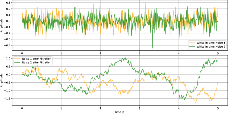
Figure 1: Comparison between white noise and filtered noise in two-dimension case. The above are two independent increment of the white Gaussian noise $dW_{1}$ and $dW_{2}$. The below are the filtered noises with $d\xi_{1}=(-0.1\xi_{1}+\xi_{2})dt+dW_{1}$ and $d\xi_{2}=(\xi_{1}-0.1\xi_{2})dt+dW_{2}$. The filters are coupled with oscillation frequency $1$ and damping rate $0.1$.

Thus, a simple way to model the effect of filtered noise is to augment the state space by a set of filter variables $\xi$ with OU dynamics. It has the advantage of keeping the model in the class of standard SDEs. But a clear consequence of such modelling is that the white noise acts only on the filter variables, not the original system, so the noise is automatically degenerate.

Note, however, that because the filter dynamics are linear, the resulting filtered noise is still Gaussian. More sophisticated approaches to modelling noise leave the Gaussian world, e.g. $t$-processes and stable processes, which have heavier tails than Gaussian, and have more than just first and second order cumulants. We do not address such extensions here.

As discussed in the previous section, a common phenomenon in various domains is the occurrence of escape from a stable equilibrium, due to forcing. In this article, we will investigate a specific circumstance: transition from a stable equilibrium to a nearby saddle, under both filtered and degenerate noise. The motivation is transition to the region on the other side of the saddle’s stable manifold, which is assumed to be of codimension one, but for small noise, the most likely route to the other side is via a set of paths that concentrate on paths that go to the saddle. In the limit of small noise, such transition become rare and are difficult to observe via direct sampling, but their probability can be expressed by Large Deviation Theory.

2.1 Large Deviation Theory

The theory of large deviations in probability theory deals with the behaviour of extreme tails of sequences of probability distributions, going beyond the domain of applicability of central limit theory. It formalises the concepts of concentration of measures and extends the notion of convergence of probability measures [27]. Here we follow the scheme from [11].

Given a generic stochastic differential equation (SDE) taking the form

$$dX_{t}=b(X_{t})dt+\sqrt{\epsilon}\sigma(X_{t})dW_{t}\quad\textrm{,}\quad X_{t}\in\mathbb{R}^{n}$$

with initial condition $X_{0}$, total time $T$ and deterministic drift $b(X_{t})$, the probability that a sample path $\{X_{t}\}^{T}_{t=0}$ is located inside a cylinder of small radius $\delta$ around a chosen path $\phi(t)$ is said to satisfy a large deviation principle if

$$\mathbb{P}(\sup_{t\in[0,T]}|X_{t}-\phi(t)|<\delta)\asymp e^{-\frac{S[\phi]}{\epsilon}}$$ (1)

when $\epsilon\rightarrow 0$, where $S[\phi]$ is a functional called a ‘rate function’. The $\asymp$ denotes that the asymptotic behaviour of both sides is equivalent when taking the logarithm:

$$\lim_{\epsilon\rightarrow 0}\epsilon\log\mathbb{P}(\sup_{t\in[0,T]}|X_{t}-\phi(t)|<\delta)=-S[\phi].$$

The action functional was derived by [8] for the case of non-degenerate noise, i.e. $C=\sigma\sigma^{T}$ positive-definite.

Theorem 1 (Freidlin-Wentzell Theorem)

The sample paths of the stochastic differential equation

$$dX_{t}=b(X_{t})dt+\sqrt{\epsilon}\sigma(X_{t})dW_{t},$$

with $X_{t}\in\mathbb{R}^{n}$, $t\in[0,T]$ satisfy a large deviation principle with rate functional

$$S[\phi]=\frac{1}{2}\int_{0}^{T}\langle\dot{\phi}-b(\phi),C^{-1}(\dot{\phi}-b(\phi))\rangle dt$$ (2)

where $\phi\in\mathbb{R}^{n}$ is any possible deterministic trajectory that an action value could be assigned to and $C(X_{t})=\sigma(X_{t})\sigma^{T}(X_{t})$ denotes the positive-definite covariance matrix.

The stated theorem provides a LDP for paths. We are interested in probability of transition, regardless of the path. The probability to hit (close to) the saddle also fulfils an LDP via a “contraction principle” [5], where the rate function is given by the minimum over all paths that reach the saddle. The only required ingredient is that the mapping from path to endpoint is continuous (which it is), the rest follows directly via contraction.

As a consequence, LDT replaces the ineffective rare event sampling problem with a deterministic optimisation problem to compute the minimiser $\phi^{*}$ of $S$. This reframing has multiple advantages: (i) the computational cost is roughly independent of the rareness of the event, whereas direct sampling of rare events becomes typically exponentially harder in the tails, (ii) the action at the minimum allows to quantify the tail scaling of the expected waiting time to observe the event, and its explicit dependence on the noise strength is known, and (iii) the trajectory $\phi^{*}$ itself represents the most likely way the rare transition is realized, allowing to identify physical mechanisms responsible for, or involved in, the transition.

However, when the noise is degenerate, the action functional (2) is ill-defined due to the loss of invertibility of the covariance matrix. To address this issue, instead of from the perspective of LDP, we use the Hamiltonian Optimal Control Method. This method provides an alternative expression for the rate functional that avoids direct inversion of the noise covariance matrix hence deals nicely with the problem of degenerate noise.

2.2 Hamiltonian Optimal Control Method

Minimising $S(\phi)$ is equivalent to an optimal control problem. We will first introduce the general optimal control result for a system of ODEs with non-degenerate forcing. This reproduces the same expression as the rate functional (2). Then we discuss the Hamiltonian optimal control method, which introduces a conjugate momentum to the system, and has no requirement for inverting the covariance matrix.

For any trajectory $\phi$ of the dynamics $\dot{\phi}=b(\phi)+\sigma\eta$ defined on $t\in[0,T]$, where $b(\phi)$ is a deterministic vector field, $\sigma$ is invertible and $\eta$ is a square-integrable forcing function, we wish to minimise its action $\frac{1}{2}\int_{0}^{T}|\eta|^{2}dt$ subject to the boundary conditions $\phi(0)=\phi_{0}$ and $\phi(T)=\phi_{T}$. This can be written as

$$\frac{1}{2}\int_{0}^{T}|\eta|^{2}dt =\frac{1}{2}\int_{0}^{T}\langle\sigma^{-1}(\dot{\phi}-b(\phi)),\sigma^{-1}(\dot{\phi}-b(\phi))\rangle dt$$

$$=\frac{1}{2}\int_{0}^{T}(\dot{\phi}-b(\phi))^{T}C^{-1}(\dot{\phi}-b(\phi))dt,$$

where $C=\sigma\sigma^{T}$. This expression yields the Freidlin-Wentzell theorem for its rate functional and corresponds to the standard optimal control approach for Lagrangian $\mathcal{L}(\phi,\dot{\phi})=\frac{1}{2}\langle\dot{\phi}-b(\phi),C^{-1}(\dot{\phi}-b(\phi))\rangle$. A necessary condition for an optimal solution is that it satisfy the Euler-Lagrange equations for this Lagrangian.

The above derivation holds only under the condition that the covariance matrix $C$ is invertible. However, in many contexts, this does not hold, as in the example we mentioned above. In such cases, the Hamiltonian Optimal Control method (which goes back to Pontryagin and is for example outlined in [11]) provides a solution to address the issue of non-invertibility. We would like to minimise $\frac{1}{2}\int_{0}^{T}|\eta|^{2}dt$ subject to the constraint $\dot{\phi}=b(\phi)+\sigma\eta$ and the boundary conditions $\phi(0)=\phi_{0}$ and $\phi(T)=\phi_{T}$. By introducing a Lagrange multiplier function $\mu$ and vector $\beta$, followed by integration by parts, the objective function can be chosen to be

$$\frac{1}{2}\int_{0}^{T}\langle\eta,\eta\rangle dt+\int_{0}^{T}\langle\mu,\dot{\phi}-b(\phi)-\sigma\eta\rangle dt+\langle\beta,(\phi(T)-\phi_{T})\rangle$$

$$= \frac{1}{2}\int_{0}^{T}(\eta^{T}\eta-\dot{\mu}^{T}\phi-\mu^{T}b(\phi)-\mu^{T}\sigma\eta)dt+\mu(T)^{T}\phi(T)-\mu(0)^{T}\phi_{0}-\beta^{T}(\phi(T)-\phi_{T}).$$

Varying with respect to $\eta$ and $\phi$ gives the following necessary conditions for finding stationary points of the above optimisation problem:

$$\eta^{T}-\mu^{T}\sigma =0,$$

$$\dot{\mu}^{T}+\mu^{T}\nabla b(\phi) =0,$$

$$\mu(T)+\beta^{T} =0.$$

Substituting $\eta=\sigma^{T}\mu$ and $C=\sigma\sigma^{T}$ one obtains

$$\dot{\phi}=b(\phi)+C\mu=\nabla_{\mu}\mathcal{H}(\phi,\mu)$$ (3)

$$\dot{\mu}=-(\nabla b(\phi))^{T}\mu=-\nabla_{\phi}\mathcal{H}(\phi,\mu).$$ (4)

This pair of equations can be viewed as the Hamilton’s equations of motion for

$$\mathcal{H}(\phi,\mu)=\langle b(\phi),\mu\rangle+\frac{1}{2}\langle\mu,C\mu\rangle,$$

which is the Legendre-Fenchel transform of the Lagrangian $\mathcal{L}(\phi,\dot{\phi})$ with respect to $\dot{\phi}$. One can solve (3) forward in time from $\phi(0)=\phi_{0}$ and solve (4) backward in time from $\mu(T)=-\beta$, and hope to vary $\beta$ until the desired final condition $\phi(T)=\phi_{T}$ is obtained. In our case the endpoint conditions could be the stable equilibrium ($\phi_{0}$) and the saddle ($\phi_{T}$) correspondingly, or points near these, as we will be interested in the limiting case of infinite time from sink to saddle. Moreover, by the forward equation (3), the action takes a simpler form:

$$S[\mu]=\frac{1}{2}\int_{0}^{T}\langle C\mu,\mu\rangle dt.$$ (5)

With this reformulation, the inverse of $C$ is no longer required and the problem is well-defined even if $\sigma$ is degenerate, namely, to minimise (5) subject to (3) and end conditions.

The above approach can be further improved by applying the Augmented Lagrangian method [14]. The point is that finding the right value of $\beta$ is not always easy and it is better to convexify the objective function. This method is based on the Lagrange Multiplier concept but replaces the above constrained optimisation problem with a series of unconstrained problems, by adding a penalty term to the objective function. In our example, this gives

$$\frac{1}{2}\int_{0}^{T}\langle\eta,\eta\rangle dt+\int_{0}^{T}\langle\mu,\dot{\phi}-b(\phi)-\sigma\eta\rangle dt+\langle\beta,(\phi(T)-\phi_{T})\rangle+\lambda||\phi(T)-\phi_{T}||^{2}.$$

Here $\beta$ is to mimic a Lagrange multiplier and $\lambda$ is the penalty parameter. The limit of $\lambda$ to infinity would guarantee the convergence to the ‘true’ solution while an algorithm for updating $\beta$

$$\beta\leftarrow\beta+\lambda\cdot c(\phi)\quad$$

makes it not necessary to take $\lambda$ to infinity, just large enough, thereby avoiding ill-conditioning. Here $c(\phi)$ is the constraint on $\phi$ which equals $c(\phi)=(\phi(T)-\phi_{T})$ in our example. The improved version avoids numerical instabilities and leads to strong theoretical convergence. Detailed derivation is given in Chapter 17 of [22]. This method only affects the pair of Hamilton equations through the boundary condition for $\mu$ in the backward equation (4) via $\phi(T)$ and $\lambda$.

Through the introduced conjugate momentum $\mu$, the Hamiltonian Optimal Control method (HOC) has tackled the issue of non-invertibility of the covariance matrix via the new action form $S[\mu]$ (5). In the derivation, $\mu$ is the Lagrange Multiplier, but also plays the role of ’noise’ in the forward equation (3). In the later context, we will denote $\theta$ as the ’noise’ in the dynamics $\dot{\phi}=b(\phi)+C\theta$ while keeping $\mu$ as the Lagrange multiplier.

3 Method of Division

While the previous section addresses the question of how to overcome complications of degenerate and coloured noise, we now turn our attention to the problem of an infinite time-horizon. To this effect, we introduce a new method in a general context, with one illustrative example and a more realistic but still simplified real-world application discussed in the subsequent section. This approach is specifically designed for handling transitions from a stable equilibrium to a saddle point, defined to be a hyperbolic equilibrium point with one-dimensional unstable manifold.

We would like to determine the probability rate for transition by computing the minimal rate functional for $T\rightarrow\infty$. However, numerical simulation over an infinite time interval is infeasible. Approximating it with a finite time interval leads to very different behaviour (if the time interval is chosen too short) or is computationally prohibitive, especially for high-dimensional systems. At the same time, any transition trajectory on an infinite time interval spends almost all its time near the fixed points, and only briefly visits the transitional region. Any equidistant discretisation of the computational time interval thus constitutes an extremly inefficient use of computational resources, where most effort is spent on regions where the dynamics are almost linear.

The proposed method, called the Method of Division, tackles the above challenges by focusing the numerics exclusively on the nonlinear transitional regime, using analytical approximations for the semi-infinite intervals near the two equilibria by their linearisations. This approach eliminates unnecessary computation near the equilibria, thus enhancing performance without sacrificing accuracy. Furthermore, the approximate dynamics around the endpoints are analysed under an infinite time scale which allows us to study the asymptotic behaviour as $\sqrt{\epsilon}\rightarrow 0$ and $T\rightarrow\infty$ in equation (1). This makes it possible to study the limiting characteristics of the transition, yielding more meaningful insights into rare event dynamics.

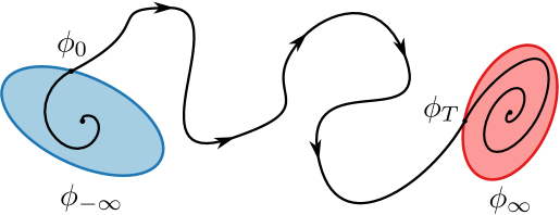
Figure 2: A sketch of the Method of Devision, where the transition process is divided into three parts: linearised dynamics around the sink $\phi_{-\infty}$ (in blue) and the saddle $\phi_{\infty}$ (in red), and the transition from $\phi_{0}$ to $\phi_{T}$.

The Method of Division divides the whole transition process into three parts:

1. Initial Escape ($\phi_{0}$): The process involves the system escaping from the neighbourhood of the stable equilibrium and moving to a point, $\phi_{0}$, near the equilibrium. This is allowed to take an infinite amount of time for interval $(-\infty,0]$.

2. Effective Transition: The core transition phase from $\phi_{0}$ to somewhere near the saddle, denoted as $\phi_{T}$. This part occurs over the finite, effective transition time $[0,T]$.

3. Final Approach: The final part in which the system moves from $\phi_{T}$ to the saddle. Like the initial escape, this part can also take an infinite amount of time for interval $[T,\infty)$.

Rather than finding the optimal trajectory connecting the fixed points, the method begins and terminates the optimal trajectory close enough to these points such that a linear approximation of the dynamics is accurate enough. See Figure [2] as a model sketch. $\phi_{-\infty}$ and $\phi_{\infty}$ represent the sink and the saddle correspondingly. The part in blue is the initial escape and the part in red is the final approach. The trajectory in between spends a finite time $T$ for effective transition. Consequently, the total action now consists of three components: the cost associated with escaping the neighbourhood of attraction, the action for the core transition as defined by the Hamiltonian Optimal Control outlined in section 2.2, and lastly the cost of overcoming the unstable direction of the saddle. Importantly, the optimisation problem for the two linear parts can be solved analytically. The Method of Division handles a more difficult question: we find not only the optimal trajectory for transition but also the optimal starting point $\phi_{0}$ and ending point $\phi_{T}$. We will detailly explain the analysis for these three processes.

Note that for trajectory $\phi$ we mean the dynamics

$$\dot{\phi}=b(\phi)+\sigma\eta,$$

where $b(\phi)$ is the deterministic flow, $\sigma$ is the diffusion matrix and $\eta$ represents the ’noise’ that is to be controlled and optimised to give the smallest overall action.

3.1 Sink

Assume without loss of generality that the sink is at the origin: $\phi_{-\infty}=\textbf{0}$. Firstly, from the sink $\phi_{-\infty}$ to $\phi_{0}$, the dynamics can be approximated by a linearised dynamics with derivative $A_{-\infty}\in\mathbb{R}^{n\times n}$, obtained by setting $A_{-\infty}=\nabla b(\textbf{0})$. The equation of motion is then $\dot{\phi}=A_{-\infty}\phi+\sigma\eta$, with boundary conditions $\phi(-\infty)=0$ and $\phi(0)=\phi_{0}$. We can express the action as the effort needed to overcome friction, with external noise influencing the system. Thus, the action for this part is: $\frac{1}{2}\int_{-\infty}^{0}|\eta(s)|^{2}ds$, subject to a constraint that this trajectory reached the point $\phi_{0}$.

The matrix $A_{-\infty}$ is assumed to be stable, i.e. all eigenvalues have negative real parts. By Duhamel’s principle (e.g. in [28]),

$$\phi(t)=\int^{t}_{-\infty}e^{A_{-\infty}(t-s)}\sigma\eta(s)\,ds.$$

In particular, we have

$$\phi(0)=\int_{-\infty}^{0}e^{-A_{-\infty}s}\sigma\eta(s)\,ds.$$

To clarify the notations used: $\phi(-\infty)$ and $\phi(0)$ refer to the starting and ending points of process 1, where $\phi(-\infty)$ is assumed to be zero and $\phi(0)$ is computed using Duhamel’s principle. On the other hand, $\phi_{0}$ represents a chosen endpoint of process 1 and is also the starting point for transition process 2.

Given $\phi_{0}$, the endpoint for the process 1, as a constraint, there is the following objective function by applying the method of Lagrange multipliers:

$$F[\phi,\eta,\epsilon] =\frac{1}{2}\int_{-\infty}^{0}|\eta(s)|^{2}ds+\langle\epsilon,(\phi_{0}-\phi(0))\rangle$$

$$=\frac{1}{2}\int_{-\infty}^{0}|\eta(s)|^{2}ds+\langle\epsilon,(\phi_{0}-\int_{-\infty}^{0}e^{-A_{-\infty}s}\sigma\eta(s)ds)\rangle$$

$$=\frac{1}{2}\int_{-\infty}^{0}\eta^{T}\eta\,ds+\epsilon^{T}(\phi_{0}-\int_{-\infty}^{0}e^{-A_{-\infty}s}\sigma\eta(s)ds)$$

$$\frac{\delta F}{\delta\eta} =\int_{-\infty}^{0}(\eta^{T}-\epsilon^{T}e^{-A_{-\infty}s}\sigma)ds=0$$

$$\eta^{T} =\epsilon^{T}e^{-A_{-\infty}s}\sigma.$$

Therefore, under the optimal trajectory and noise:

$$\phi(0)=\int_{-\infty}^{0}e^{-A_{-\infty}s}\sigma\sigma^{T}e^{-A_{-\infty}^{T}s}\lambda ds=Q\lambda,$$

$$\frac{1}{2}\int_{-\infty}^{0}|\eta(s)|^{2}ds=\frac{1}{2}\int_{-\infty}^{0}\lambda^{T}e^{-A_{-\infty}s}\sigma\sigma^{T}e^{-A_{-\infty}^{T}s}\lambda ds=\frac{1}{2}\lambda^{T}Q\lambda,$$

where

$$Q=\int_{-\infty}^{0}e^{-A_{-\infty}s}\sigma\sigma^{T}e^{-A_{-\infty}^{T}s}ds.$$

A convenient way to compute $Q$ is to note that it satisfies the Lyapunov equation $A_{-\infty}Q+QA_{-\infty}^{T}=\sigma\sigma^{T}$. As $A_{-\infty}$ is contracting, the solution to this Lyapunov equation is unique [1] and can be computed by standard routines. Furthermore, assuming controllability of the linearised dynamics around the sink ensures that Q is invertible [28]. Since at the constraint $\phi(0)=\phi_{0}$, we can express $\lambda$ as $\lambda=Q^{-1}\phi_{0}$. This leads to a further simplification of the action expression:

$$\frac{1}{2}\int_{-\infty}^{0}|\eta(s)|^{2}ds=\frac{1}{2}\phi_{0}^{T}Q^{-1}\phi_{0}.$$

Given a chosen $\phi_{0}$, we have the optimal $\eta$ such that the trajectory from the stable equilibrium $\phi(-\infty)$ to $\phi_{0}$ is deterministic. By substituting $s=t+\tau$, we can explicitly express $\phi(t)$ as

$$\phi(t) =\int_{-\infty}^{t}e^{A_{-\infty}(t-s)}\sigma\eta(s)\,ds$$

$$=e^{A_{-\infty}t}\int_{-\infty}^{t}e^{-A_{-\infty}s}\sigma\sigma^{T}e^{-A_{-\infty}^{T}s}\lambda\,ds$$

$$=e^{A_{-\infty}t}\int_{-\infty}^{0}e^{-A_{-\infty}(t+\tau)}\sigma\sigma^{T}e^{-A_{-\infty}^{T}(t+\tau)}\lambda\,d\tau$$

$$=\int_{-\infty}^{0}e^{-A_{-\infty}\tau}\sigma\sigma^{T}e^{-A_{-\infty}^{T}\tau}e^{-A_{-\infty}^{T}t}\lambda\,d\tau$$

$$=Qe^{-A_{-\infty}^{T}t}\lambda$$

$$=Qe^{-A_{-\infty}^{T}t}Q^{-1}\phi_{0}.$$ (6)

The final equation is fully specified, leaving no unknowns, which allows for an easy sketch of the linearised dynamics. Equivalently, the optimally controlled dynamics for the linearised system around the sink is given by

$$\dot{\phi}=-QA_{-\infty}^{T}Q^{-1}\phi.$$

3.2 Saddle

Similarly to the case of a sink, we can linearly approximate the dynamics around the saddle s using a matrix $A_{\infty}$ obtained by evaluating $\nabla b(\phi)$ at the saddle s. For simplicity, let us first shift the saddle to the origin 0. An equation that includes the effect of shifting the saddle will be given at the end of this subsection. The saddle has $n-1$ eigenvalues with negative real parts and one positive eigenvalue $\lambda_{+}>0$.

It is convenient to analyse the linearised system in a coordinate system that separates off the unstable direction. Thus, we define a projection $P$ by $P=rl^{T}$ where $r$ and $l$ are the corresponding right and left eigenvectors of the positive (unstable) eigenvalue $\lambda_{+}$ (normalised to have $l^{T}r=1$). This projection decomposes the space into $E_{s}\oplus E_{u}$, where $E_{u}=$ Im($P$) and $E_{s}=$ Ker($P$). At least one component of $l$ is non-zero, without loss of generality the first. Define a transformation matrix $U$ as

$$U=\begin{pmatrix}r_{1}&-\frac{l_{2}}{l_{1}}&-\frac{l_{3}}{l_{1}}&...&-\frac{l_{n}}{l_{1}}\\ r_{2}&1&0&...&0\\ r_{3}&0&1&...&0\\ ...&...&...&...&0\\ r_{n}&0&0&...&1\end{pmatrix}.$$

The image by $U$ of the first unit vector is $r$, and $l^{T}U$ is the row vector $[1,0,\ldots 0]$. This transforms $A_{\infty}$ into a matrix $\tilde{A}=U^{-1}A_{\infty}U$ taking the block form

$$\tilde{A}=\begin{pmatrix}\begin{array}[]{c|c}\tilde{A_{u}}&0\\ \hline\cr 0&\widetilde{A}_{s}\end{array}\end{pmatrix}=\begin{pmatrix}\begin{array}[]{c|c}\lambda_{+}&0\\ \hline\cr 0&\widetilde{A}_{s}\end{array}\end{pmatrix},$$

where $\tilde{A_{s}}\in\mathbb{R}^{(n-1)\times(n-1)}$ is a stable matrix. Compared to diagonalisation, this transformation defined by $U$ is more efficient (it does not require computation of the other eigenvectors) and robust (diagonalisation is unstable near cases of repeated eigenvalues, and in general impossible if there are any repeated eigenvalues). There is freedom to apply any invertible coordinate change to the $(n-1)\times(n-1)$ block, if desired, but we did not use that.

Thus, by changing the coordinates and writing $U^{-1}(\phi-\textbf{s})=\tilde{\phi}$, the linearised dynamics is then equivalent to

$$U^{-1}\dot{\phi} =U^{-1}A_{\infty}\phi+U^{-1}\sigma\eta$$

$$\dot{\tilde{\phi}} =\tilde{A}\tilde{\phi}+\tilde{\sigma}\eta,$$

where $\tilde{\sigma}=U^{-1}\sigma$. Since $\tilde{A}$ is in block form, this can be decomposed as

$$\dot{\tilde{\phi^{1}}} =\lambda_{+}\tilde{\phi^{1}}+\tilde{\sigma}^{1}\eta,$$

$$\dot{\tilde{\phi^{i}}} =(\tilde{A_{s}}\tilde{\phi})^{i}+\tilde{\sigma}^{i}\eta\text{,\quad\quad\quad for $2\leq i\leq n$}.$$

Note that, to travel from the endpoint $\phi_{T}$ to the saddle, external force is only required for the $\phi_{1}$ component. For the components along the stable manifold, the dynamics will naturally flow toward the saddle, as long as the optimal noise $\eta$ associated with the unstable component goes to zero.

Hence, we aim to find an optimal $\eta$ such that for $0\leq t\leq\infty$, the dynamics satisfies $\tilde{\phi^{1}}(0)=\tilde{\phi^{1}}_{\text{end}}$ and $\tilde{\phi^{1}}(\infty)=0$. By Duhamel’s Principle, $\tilde{\phi^{1}}(0)=-\int_{0}^{\infty}e^{-\lambda_{+}s}\tilde{\sigma^{1}}\eta(s)\,ds$, where $\tilde{\sigma}^{1}$ denotes the first row of $\tilde{\sigma}$. Minimising $\frac{1}{2}\int^{\infty}_{0}|\eta|^{2}dt$ subject to the boundary conditions employing the Lagrangian Multiplier method gives:

$$G[\tilde{\phi^{1}}]=\frac{1}{2}\int^{\infty}_{0}|\eta(s)|^{2}ds+\beta(\tilde{\phi}^{1}_{\text{end}}-\tilde{\phi^{1}}(0)).$$

By similar computation as in the sink case,

$$\eta =-(\tilde{\sigma}^{1})^{T}e^{-\lambda_{+}s}\beta,$$

$$\beta =\frac{\tilde{\phi}^{1}_{\text{end}}}{q},$$

$$\frac{1}{2}\int^{\infty}_{0}|\eta|^{2}dt =\frac{1}{2}q^{-1}(\tilde{\phi}^{1}_{\text{end}})^{2},$$

where $q\in\mathbb{R}$ is given by

$$q=\int^{\infty}_{0}e^{-\lambda_{+}s}(\tilde{\sigma}^{1})(\tilde{\sigma}^{1})^{T}e^{-\lambda_{+}s}ds=\frac{(\tilde{\sigma}^{1})(\tilde{\sigma}^{1})^{T}}{2\lambda_{+}}.$$

Assuming controllability of the linearised dynamics around the saddle, $q$ is non-zero. Hence, with a given $\tilde{\phi}_{\text{end}}$ and the optimal noise $\eta$, the controlled dynamics is

$$\hat{A}=\begin{pmatrix}\begin{array}[]{c|c}-\lambda_{+}&0\\ \hline\cr-q^{-1}(\tilde{\sigma}^{i})(\tilde{\sigma}^{1})^{T}&\tilde{A_{s}}\end{array}\end{pmatrix}$$

where the $i^{th}$ entry of the first column is given by $-(\tilde{\sigma}^{i})(\tilde{\sigma}^{1})^{T}q^{-1}$ for $2\leq i\leq 6$. $\hat{A}$ is now contracting. The trajectory for the unstable component takes the form

$$\tilde{\phi}^{1}(t)=\tilde{\phi^{1}}_{\text{end}}e^{-\lambda_{+}t},$$ (7)

and the trajectories for the stable components are

$$\tilde{\phi_{i}}(t)=(e^{\tilde{A_{s}}t}\tilde{\phi}^{\text{end}})_{i}-\tilde{\sigma_{i}}\tilde{\sigma_{1}}^{T}q^{-1}e^{-\lambda_{+}t}\tilde{\phi_{1}}^{\text{end}}$$ (8)

for $i=2\leq i\leq n$. These trajectories can be transformed back to the original coordinate by $\phi=U\tilde{\phi}+\textbf{s}$. Detailed computation for the analysis around the saddle is in the Appendix A.

A question worth asking is how to choose the point $\phi_{\text{end}}$ or in transformed coordinate $\tilde{\phi}_{\text{end}}$? It should be close enough to the saddle so that the linearisation error remains negligible. On the other hand, all stable components make no contribution to the action, so there is freedom to choose the point. Consider an ellipsoid centred at the saddle, defined by $(\tilde{\phi}^{\text{end}})^{T}M(\tilde{\phi}^{\text{end}})-r^{2}=0$ for some positive-definite matrix $M$, such that the optimally controlled dynamics is transverse to the ellipsoid. This ellipsoid restricts an area around the saddle that is small enough for the accuracy of the linearisation approximation. The overall optimisation problem finds an optimal point on the ellipsoid to enter this domain and the motion within this domain is purely analytical. To achieve the transversality, we choose the matrix $M$ to satisfy the Lyapunov equation $\hat{A}^{T}M+M\hat{A}+I_{n}=0$, where $I_{n}$ is the n-dimensional identity matrix, but could be any other positive-definite matrix and $\hat{A}$ is the transformed linearised dynamics under control. Because $\hat{A}$ is contracting, $M$ is positive definite.

3.3 Overall Problem

The analysis of transition process 2 employs the Hamiltonian Optimal Control method discussed in the previous section, where the action is in the parametrised format. Then the optimisation problem is to minimise the overall action:

$$S[\phi,\theta]=\frac{1}{2}\phi_{0}^{T}Q^{-1}\phi_{0}+\frac{1}{2}\int_{0}^{T}\langle a\theta(t),\theta(t)\rangle\,dt+\frac{1}{2}q^{-1}(U^{-1}(\phi(T)-\textbf{s}))_{u}^{2}$$

where $(U^{-1}(\phi(T)-\textbf{s}))_{1}$ is the unstable component of the optimal endpoint. The three terms correspond to the action from the three processes by the Method of Division, where only the middle term is expressed explicitly as an integral over time $t\in[0,T]$. The first term is determined by the initial escape state where the action can be expressed in terms of the starting point of the trajectory $\phi$ at $t=0$. The third term is from the final approach state, where only the unstable component of the end point of the trajectory $\phi(t=T)$ is relevant. The function $S[\phi,\theta]$ is our rate functional in the Large Deviation Principle for computing the probability.

These actions are minimised subject to the following constraints:

$$\phi_{0}=\phi(0),$$ (9)

$$\dot{\phi}=b(\phi)+a\theta,$$ (10)

$$r^{2}=\tilde{\phi}(T)^{T}M\tilde{\phi}(T).$$ (11)

Constraint (9) forces that the transition begins at the starting point $\phi_{0}$ near the sink that is to be optimised. Constraint (11) mandates that the transition ends on an ellipsoid, with $\tilde{\phi}(T)=U^{-1}(\phi(T)-\textbf{s})$ expressed in the transformed coordinate. Constraint (10) is the forward equation of the Hamiltonian method for the transition.

3.3.1 Algorithm and Numerical Solutions

To solve this optimisation problem, we apply the Augmented Lagrangian method, the objective cost function is:

$$J[\phi,\theta,\mu,\epsilon,\beta,\lambda]= \frac{1}{2}\phi_{0}^{T}Q^{-1}\phi_{0}+\frac{1}{2}\int_{0}^{T}\langle a\theta,\theta\rangle dt+\frac{1}{2}q^{-1}\tilde{\phi}(T)_{1}^{2}+\langle\epsilon,\phi_{0}-\phi(0)\rangle$$

$$+\int_{0}^{T}\langle\mu,\dot{\phi}-b(\phi)-a\theta\rangle dt+\beta(\tilde{\phi}(T)^{T}M\tilde{\phi}(T)-r^{2})+\lambda(\tilde{\phi}(T)^{T}M\tilde{\phi}(T)-r^{2})^{2}.$$

The parameters $\epsilon\in\mathbb{R}^{n},\mu\in\mathbb{R}^{n},\beta\in\mathbb{R}$ are the Lagrange multipliers and $\lambda\in\mathbb{R}$ is a penalty parameter. Note that $\phi(0)$ and $\phi(T)$ correspond to the initial point and endpoint of the trajectory in process 2. For convenience, we can substitute $\phi(0)=\phi_{1}$ and $\phi(T)=\phi_{N}$ when discretising the trajectory $\phi$ into $N$ segments. A detailed discretisation scheme is given in the Appendix B.

Varying the discretised cost function $J$ with respect to the variables $\phi_{0}$, $\theta$ and $\phi$ gives:

$$\frac{dJ}{d\phi_{0}} =Q^{-1}\phi_{0}+\epsilon$$

$$\frac{dJ}{d\theta} =a(\theta-\mu)$$

$$\frac{dJ}{d\phi_{1}} =-\epsilon-\mu_{1}-\mu_{1}\nabla b(\phi_{1})^{T}\Delta t$$

$$\frac{dJ}{d\phi_{i}} =\mu_{i-1}-\mu_{i}-\mu_{i}\nabla b(\phi_{i})^{T}\Delta t$$

$$\frac{dJ}{d\phi_{N}} =\mu_{N-1}+2(U^{-T}MU^{-1})(\phi_{N}-\textbf{s})(\beta+2\lambda(\tilde{\phi}_{N}^{T}M\tilde{\phi}_{N}-r^{2})).$$

This follows a very similar idea as discussed in the Hamiltonian Optimal Control method: the constraint and the penalty term on the ellipsoid together provide the boundary condition for the backward Hamiltonian equation (4) on $\mu$. The introduced conjugate momentum $\theta$ is updated via gradient $a(\theta-\mu)$ so that $\theta$ and $\mu$ are equivalent at the optimal. The backward equation on $\mu$ further gives a condition on $\epsilon$ so that $\phi_{0}$ can be optimised. Hence, we have two variables to optimise: $\phi_{0}$ and $\theta$ where $\theta$ depends on time $t\in[0,T]$. The trajectory $\phi$ can be computed from $\phi_{0}$, knowing $\theta$, through the forward Hamilton’s equation (3), and the endpoint $\phi_{N}$ is forced on the ellipsoid that gives the smallest action. The algorithm is as follows:

1. Initialise $\phi_{0}$, $\theta$, and penalty parameters $(\beta,\lambda)$ with constant $1<c<2$.

2. Fix the penalty parameters and update $\phi_{0}$ and $\theta$:

   1. Solve the forward Hamiltonian dynamics

      $$\dot{\phi}=b(\phi)+a\theta,\quad\phi(0)=\phi_{0},$$

      on $[0,T]$ to obtain $\phi(T)$.

   2. Solve the backward adjoint dynamics

      $$\dot{\mu}=-\nabla b(\phi)^{\top}\mu,$$

      with terminal condition

      $$\mu_{N-1}=-2(U^{-T}MU^{-1})(\phi(T)-\mathbf{s})\bigl(\beta+2\lambda(\tilde{\phi}(T)^{\top}M\tilde{\phi}(T)-r^{2})\bigr),$$

      to obtain $\mu$ and $\epsilon$ with

      $$\epsilon=-\mu_{1}-\mu_{1}\nabla b(\phi_{1})^{T}\Delta t.$$

   3. Update the parameters via gradient descent:

      $$\theta\leftarrow\theta-\alpha_{\theta}\,a(\theta-\mu),\quad\phi_{0}\leftarrow\phi_{0}-\alpha_{\phi}(Q\phi_{0}+\epsilon).$$

      for some step sizes $\alpha_{\theta}$ and $\alpha_{\phi}$. Detailed discussion on the norm of the gradient is in Appendix C.

   4. Repeat steps (a)-(c) until the norm of the overall gradient is sufficiently small.

3. Update the penalty parameters:

   $$\beta\leftarrow\beta+\lambda(\tilde{\phi}(T)^{\top}M\tilde{\phi}(T)-r^{2}),\quad\lambda\leftarrow c\lambda.$$

   Repeat step 2 until the endpoint $\phi(T)$ lies sufficiently close to the ellipsoid

Output: Optimised $\theta$ and $\phi_{0}$.

4 Examples

4.1 Inverted Double Well

Consider an inverted double well model with potential $V(x)=\frac{1}{2}x^{2}-\frac{1}{4}x^{4}$. The Newton’s equation of motion for a particle with mass $m$ in this potential is $m\ddot{x}=x^{3}-x$. For simplicity, assume $m=1$. To better illustrate the method of division, let us make this a damped system with damping coefficient $k$ and add degenerate and the simplest filtered noise to the model:

$$dx =y\,dt$$

$$dy =(x^{3}-x-ky+z)dt$$

$$dz =(-z)dt+\sqrt{\epsilon}\,dW,$$

where $k$ is a positive constant denoting the damping coefficient, and $z$ is the one-dimensional filtered noise added. White-in-time noise is only added to the last line, which gives degenerate noise for the system as a whole, i.e, the covariance matrix is singular.

The above simultaneous equations could also be expressed in the generic stochastic differential equation format as

$$d\phi=b(\phi)dt+\sigma dW,\quad\text{with}\quad\phi=\begin{pmatrix}x\\ y\\ z\end{pmatrix}\quad\text{and}\quad\sigma=\begin{pmatrix}0\\ 0\\ \sqrt{\epsilon}\end{pmatrix}.$$

The deterministic dynamics of this system have three equilibrium points: the stable equilibrium $(0,0,0)$ and the two saddles $\pm(1,0,0)$. Due to symmetry, consider only one saddle at $(1,0,0)$. The linearised dynamics $\nabla b$ around the two critical points are given by

$$A_{-\infty}=\begin{pmatrix}0&1&0\\ -1&-k&1\\ 0&0&1\end{pmatrix},\quad A_{\infty}=\begin{pmatrix}0&1&0\\ 2&-k&1\\ 0&0&1\end{pmatrix}.$$ (12)

Choose $k<1$ such that the sink has one negative real eigenvalue and two complex eigenvalues with small negative real parts. The saddle has one positive real eigenvalue and two negative real eigenvalues.

The transition problem is to find the probability rate to escape towards one of the saddles if the system starts at the origin, as well as the trajectory it would take. Figure 3 illustrates the result by the Method of Division. In figure 3(a), the Hamiltonian $H(x,y)=V(x)+\frac{y^{2}}{2}$ for the undamped system is sketched as energy level sets. Note the Hamiltonian $H(x,y)$ is in the sense of mechanics and is different from the Hamiltonian of the optimal control method mentioned before. Figure 3(c) is the 3D graphs with the ellipsoid defined around the saddle. The dashed pink line is the linearised trajectory within the ellipsoid. Figure 3(b) and Figure 3(d) show the filtered noise dimension and the corresponding Gaussian white noise, where the linear part (light green) and non-linear part (dark green) are joined smoothly.

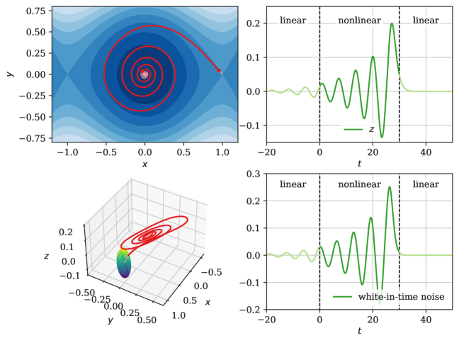
Figure 3: The optimal trajectory from the sink to the saddle in three sections: linearised dynamics at both ends and non-linear dynamics for the transition.

4.2 Ship Capsize Model

A more complicated example is a simple two degree of freedom ship capsize model, proposed by [23]. This archetypal capsize equation of the ship is designed for the beam sea, where waves travel perpendicular to the body of the ship. It has two degrees of freedom: the heave $z$ and the roll $\alpha$ (see Figure 4). The ship potential is given by

$$V(\alpha,z)=\frac{1}{2}c\alpha_{c}^{2}[(\frac{\alpha}{\alpha_{c}})^{2}-\frac{1}{2}(\frac{\alpha}{\alpha_{c}})^{4}]+\frac{1}{2}h[z-\frac{1}{2}\gamma\alpha^{2}]^{2}.$$

The roll and heave natural frequency of the ship is proportional to $\sqrt{c}$ and $\sqrt{h}$, respectively. Here, $\gamma$ is a ship parameter that is determined to best fit the ship, and $\alpha_{c}$ denotes the capsize angle. The restoring force in heave is $-\partial V/\partial z$ and the restoring moment in roll is $-\partial V/\partial\alpha$. All variables are non-dimensionalised. Then by distinguishing the moment dimension and the configuration dimension and by adding damping to heave and roll, we obtain a six-dimensional stochastic dynamical system:

$$\dot{z}=z_{v}$$

$$\dot{z}_{v}=\frac{h}{m}(\frac{1}{2}\gamma\alpha^{2}-z)-k_{1}z_{v}+B_{11}\xi_{1}+B_{12}\xi_{2}$$

$$\dot{\alpha}=\alpha_{v}$$

$$\dot{\alpha}_{v}=\frac{c}{I}\alpha(\frac{\alpha^{2}}{\alpha_{c}^{2}}-1)+\frac{h}{I}\gamma\alpha(z-\frac{1}{2}\gamma\alpha^{2})-k_{2}\alpha_{v}+B_{21}\xi_{1}+B_{22}\xi_{2}$$

$$\dot{\xi}_{1}=A_{11}\xi_{1}+A_{12}\xi_{2}+\sqrt{\epsilon}\sigma_{11}\eta_{1}+\sqrt{\epsilon}\sigma_{12}\eta_{2}$$

$$\dot{\xi}_{2}=A_{21}\xi_{1}+A_{22}\xi_{2}+\sqrt{\epsilon}\sigma_{21}\eta_{1}+\sqrt{\epsilon}\sigma_{22}\eta_{2}$$

where $z_{v}$ and $\alpha_{v}$ are the momentum dimensions. The variables $\xi_{i}$ are the added filtered noise and $\eta_{i}$ are the ’derivative’ of independent Wiener processes - so the system has filtered and degenerate noise.

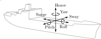
Figure 4: 6 degrees of freedom of a ship

Similarly to the inverted double well example, this system has three equilibrium points, a stable equilibrium at the origin $\textbf{0}\in\mathbb{R}^{6}$ and two saddle points at $(z,z_{v},\alpha,\alpha_{v},\xi_{1},\xi_{2})=(\frac{1}{2}\gamma\alpha_{c}^{2},0,\pm\alpha_{c},0,0,0)$ for some constant $\alpha_{c}$. The saddles have a 1-dimensional unstable manifold and a 5-dimensional stable manifold in the relevant parameter range. The special structure and symmetry of the saddles is due to its physical intuition: the ship loses balance and capsizes when it swings too severely to the left or the right. This instability comes only from the roll direction $\alpha$ and $\pm\alpha_{c}$ is the corresponding capsize angle.

Figures 5 show representative results for the ship capsize problem. The red curves indicate the optimal capsize trajectory—i.e., the most likely path to capsize—while the pink curves illustrate the linearised dynamics near the equilibrium points. In both cases, the linearised dynamics align well with the nonlinear dynamics at the boundaries. The blue and green curves represent noise: filtered noise applied to the heave and roll, and white noise applied to the filtered dimensions.

In Figure 5(a), the effective transition time is $T=20$, whereas in Figure 5(b) it is $T=30$, with all other parameters held fixed. The resulting trajectories are very similar; however, as $T$ increases, the transition from the linearised to the nonlinear regime occurs closer to the sink. This highlights the numerical advantage of the Method of Division: one can identify a sufficient transition time $T^{*}$ such that for any $T>T^{*}$, the trajectory $\phi[T]$ closely resembles $\phi[T^{*}]$, differing only by extending further within the linearised region near the sink. This saves computation cost to a great extend when investigating the change to the trajectory for longer $T$. It is also worth noting that, while the trajectories remain similar, the corresponding noise differ significantly.

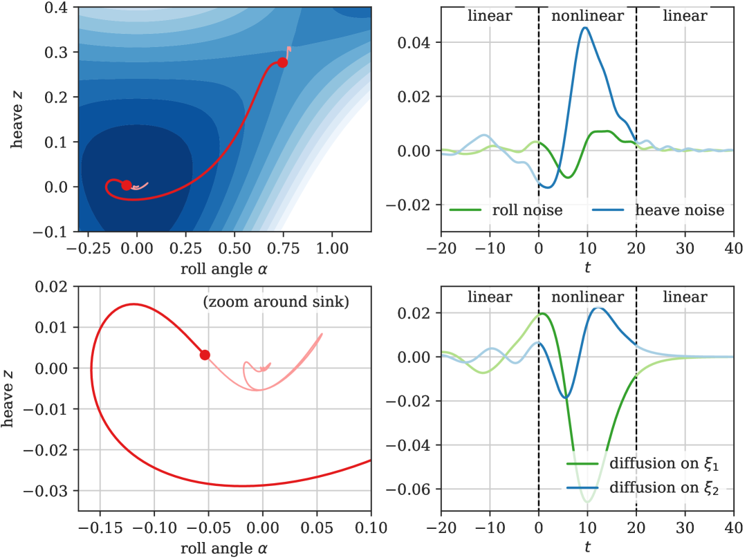
(a) transition time $T=20$

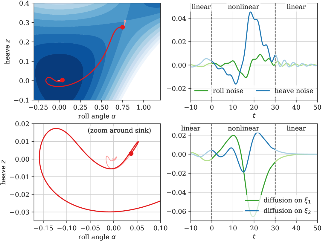
(b) transition time $T=30$

Figure 5: A comparison between two ship capsize trajectories and their corresponding optimal noise under different effective transition time. The diffusion on $\xi_{i}$ means the $i$ dimension of the correlated white Gaussian noise $\sqrt{\epsilon}\sigma_{i1}\eta_{1}+\sqrt{\epsilon}\sigma_{i2}\eta_{2}$.

5 Conclusion

In this paper, we introduced the Method of Division to address transition problems in stochastic dynamical systems over an unbounded time-scale and demonstrated its effectiveness through two examples: an inverted double well and a ship capsize problem. The proposed method accommodates both filtered and degenerate noise, making it more adaptable to real-world scenarios. It also enables an infinite time scale by focusing computational effort on the nonlinear transition phase. We illustrated the method with a transition from a stable sink to a saddle with a one-dimensional unstable manifold and discussed its broader applicability. This approach can be generalized to other disciplines with different stability structures, as transition problems arise across a wide range of fields.

Appendix A Saddle Analysis

The transformed dynamics around the saddle are given by

$$\dot{\tilde{\phi_{1}}} =\lambda_{+}\tilde{\phi_{1}}+\tilde{\sigma}_{1}\eta$$

$$\dot{\tilde{\phi_{i}}} =(\tilde{A_{s}}\tilde{\phi})_{i}+\tilde{\sigma}_{i}\eta\text{\quad\quad\quad for $2\leq i\leq n$}$$

where the first component is the unstable direction. Assume without loss of generality that the saddle is located at the origin. We aim to find an optimal $\eta$ such that for $0\leq t\leq\infty$, the dynamics satisfies $\tilde{\phi_{1}}(0)=\tilde{\phi_{1}}^{\text{end}}$ and $\tilde{\phi_{1}}(\infty)=0$. By Duhamel’s principle

$$\tilde{\phi_{1}}(t) =e^{\lambda_{+}t}\tilde{\phi_{1}}(0)+\int_{0}^{t}e^{\lambda_{+}(t-s)}\tilde{\sigma_{1}}\eta(s)ds$$

$$e^{-\lambda_{+}t}\tilde{\phi_{1}}(t) =\tilde{\phi_{1}}(0)+\int_{0}^{t}e^{-\lambda_{+}s}\tilde{\sigma_{1}}\eta(s)ds$$

Taking limitation of $t\rightarrow\infty$ on both sides would give $\tilde{\phi_{1}}(0)=-\int_{0}^{\infty}e^{-\lambda_{+}s}\tilde{\sigma_{1}}\eta(s)ds$ since $\raisebox{2.15277pt}{\scalebox{0.8}{$\displaystyle\lim_{t\rightarrow\infty}\;$}}e^{-\lambda_{+}t}\tilde{\phi_{1}}(t)=0$. Now, similar to the analysis for the sink, using the Lagrangian Multiplier method:

$$G[\tilde{\phi_{1}}] =\frac{1}{2}\int^{\infty}_{0}|\eta(s)|^{2}ds+\beta(\tilde{\phi}_{1}^{\text{end}}-\tilde{\phi_{1}}(0))$$

$$=\frac{1}{2}\int^{\infty}_{0}|\eta(s)|^{2}ds+\beta(\tilde{\phi}_{1}^{\text{end}}+\int_{0}^{\infty}e^{-\lambda_{+}s}\tilde{\sigma_{1}}\eta(s)ds)$$

$$\frac{\delta G}{\delta\eta} =\int_{0}^{\infty}(\eta^{T}+\beta e^{-\lambda_{+}s}\tilde{\sigma_{1}})ds=0$$

$$\eta =-\beta e^{-\lambda_{+}s}\tilde{\sigma_{1}}^{T}$$

Then the action around the saddle is

$$\frac{1}{2}\int^{\infty}_{0}|\eta|^{2}dt =\frac{\beta^{2}}{2}\int^{\infty}_{0}e^{-\lambda_{+}s}(\tilde{\sigma})_{1}(\tilde{\sigma})_{1}^{T}e^{-\lambda_{+}s}ds$$

$$=\frac{\beta^{2}}{2}\frac{(\tilde{\sigma})_{1}(\tilde{\sigma})_{1}^{T}}{2\lambda_{+}}$$

$$=\frac{\beta^{2}}{2}q$$

where $q=\int^{\infty}_{0}e^{-\lambda_{+}s}(\tilde{\sigma})_{1}(\tilde{\sigma})_{1}^{T}e^{-\lambda_{+}s}ds$. As under the optimal $\eta$, we have $\tilde{\phi_{1}}(0)=\tilde{\phi_{1}}^{\text{end}}$

$$\tilde{\phi_{1}}^{\text{end}} =\int_{=}^{\infty}e^{-\lambda_{+}s}\tilde{\sigma_{1}}\tilde{\sigma_{1}}^{T}e^{-\lambda_{+}s}\beta ds$$

$$=q\beta$$

Then $\beta=q^{-1}\tilde{\phi_{1}}^{\text{end}}$ and that the action takes the form $\frac{1}{2}q^{-1}(\tilde{\phi_{1}}^{\text{end}})^{2}$. Moreover, the dynamics of the unstable component at time $t$ can be explicitly written as

$$\tilde{\phi_{1}}(0) =-\int_{0}^{\infty}e^{-\lambda_{+}s}\tilde{\sigma_{1}}\eta ds$$

$$e^{\lambda_{+}t}\tilde{\phi_{1}}(0) =-\int_{0}^{\infty}e^{\lambda_{+}(t-s)}\tilde{\sigma_{1}}\eta ds$$

$$\tilde{\phi_{1}}(t) =-\int_{0}^{\infty}e^{\lambda_{+}(t-s)}\tilde{\sigma_{1}}\eta ds+\int_{0}^{t}e^{\lambda_{+}(t-s)}\tilde{\sigma_{1}}\eta ds$$

$$=-\int_{t}^{\infty}e^{\lambda_{+}(t-s)}\tilde{\sigma_{1}}\eta ds$$

$$=\int_{t}^{\infty}e^{\lambda_{+}(t-s)}\tilde{\sigma_{1}}\tilde{\sigma_{1}}^{T}e^{-\lambda_{+}s}\beta ds$$

$$=e^{-\lambda_{+}t}\int_{0}^{\infty}e^{-\lambda_{+}\tau}\tilde{\sigma_{1}}\tilde{\sigma_{1}}^{T}e^{-\lambda_{+}\tau}\beta d\tau$$

$$=e^{-\lambda_{+}t}q\tilde{\phi_{1}}^{\text{end}}q^{-1}$$

$$=\tilde{\phi_{1}}^{\text{end}}e^{-\lambda_{+}t}$$

where we have substituted $s=t+\tau$ to shift the limit of the integral. This optimised $\eta$ fully determines the trajectory for the stable components in the following manner, for $2\leq i\leq 6$:

$$\tilde{\phi_{i}} =(\tilde{A_{s}}\tilde{\phi})_{i}+\tilde{\sigma_{i}}\eta$$

$$=(\tilde{A_{s}}\tilde{\phi})_{i}-\tilde{\sigma_{i}}\tilde{\sigma_{1}}^{T}e^{-\lambda_{+}s}\tilde{\phi_{1}}^{\text{end}}q^{-1}$$

$$=(\tilde{A_{s}}\tilde{\phi})_{i}-\tilde{\sigma_{i}}\tilde{\sigma_{1}}^{T}q^{-1}\tilde{\phi_{1}}(s)$$

Hence the linearised dynamics under control is denoted by

$$\hat{A}=\begin{pmatrix}\begin{array}[]{c|c}-\lambda_{+}&0\\ \hline\cr-q^{-1}\tilde{\sigma_{i}}\tilde{\sigma_{1}}^{T}&\tilde{A_{s}}\end{array}\end{pmatrix}$$

where the $i^{th}$ entry of the first column is given by $-\tilde{\sigma_{i}}\tilde{\sigma_{1}}^{T}q^{-1}$ for $2\leq i\leq 6$. Hence, the trajectories sketched out by the stable components are

$$\tilde{\phi_{i}}(t)=(e^{\tilde{A_{s}}t}\tilde{\phi}^{\text{end}})_{i}-\tilde{\sigma_{i}}\tilde{\sigma_{1}}^{T}q^{-1}e^{-\lambda_{+}t}\tilde{\phi_{1}}^{\text{end}}$$

The point $\tilde{\phi}^{\text{end}}$ lies on the ellipsoid and is to be optimised for the overall problem.

Appendix B Discretised Gradient

The objective cost function $J$ in its discrete version takes the form

$$J[\phi,\theta,\mu,\epsilon,\beta,\lambda]= \frac{1}{2}\sum_{i,j=1}^{n}\phi_{0}^{i}Q^{-1}_{ij}\phi_{0}^{j}+\frac{1}{2}\sum_{k=1}^{N-1}(\sum_{i,j=1}^{n}(a_{ij}\theta_{k}^{j})\theta_{k}^{i})\Delta t+\frac{1}{2}q^{-1}\tilde{\phi}(T)_{u}^{2}$$

$$+\sum_{i=1}^{n}\epsilon_{i}(\phi_{0}^{i}-\phi(0)^{i})+\sum_{k=1}^{N-1}\sum_{i,j=1}^{n}\mu_{k}^{i}(\dot{\phi}_{k}^{i}-b(\phi_{k}^{i})-a_{ij}\theta_{k}^{j})\Delta t$$

$$+\beta(\sum_{i,j=1}^{n}\tilde{\phi}(T)^{i}M_{ij}\tilde{\phi}(T)^{j}-r^{2})+\lambda(\sum_{i,j=1}^{n}\tilde{\phi}(T)^{i}M_{ij}\tilde{\phi}(T)^{j}-r^{2})^{2}$$

where $n$ is the dimension of the SDE that $\phi\in\mathbb{R}^{n}$ and the total transition time $T$ is discretised into $N$ points such that $\phi_{1}=\phi(t=0)$ and $\phi_{N}=\phi(t=T)$. The Lagrangian multiplier $\mu$ is correspondingly discretised into $N-1$ points. The reason that $\mu$ has one point less than $\phi$ will be explained later. Also note that, under the transformation, $\tilde{\phi}_{N}=U^{-1}(\phi_{N}-\text{saddle})$. Then the above equation is equivalent to

$$J[\phi]= \frac{1}{2}\sum_{i,j=1}^{n}\phi_{0}^{i}Q^{-1}_{ij}\phi_{0}^{j}+\frac{1}{2}\sum_{k=1}^{N-1}(\sum_{i,j=1}^{n}(a_{ij}\theta_{k}^{j})\theta_{k}^{i})\Delta t+\frac{1}{2}q^{-1}(\tilde{\phi}_{N})_{u}^{2}$$

$$+\sum_{i=1}^{n}\epsilon_{i}(\phi_{0}^{i}-\phi_{1}^{i})+\sum_{k=1}^{N-1}\sum_{i,j=1}^{n}\mu_{k}^{i}(\frac{\phi^{i}_{k+1}-\phi^{i}_{k}}{\Delta t}-b(\phi_{k}^{i})-a_{ij}\theta_{k}^{j})\Delta t$$

$$+\beta(\sum_{i,j=1}^{n}\tilde{\phi}_{N}^{i}M_{ij}\tilde{\phi}_{N}^{j}-r^{2})+\lambda(\sum_{i,j=1}^{n}\tilde{\phi}_{N}^{i}M_{ij}\tilde{\phi}_{N}^{j}-r^{2})^{2}$$

Varying $J$ with respect to $\phi_{0}$ and $\theta$ gives:

$$\frac{dJ}{d\phi_{0}^{i}} =\sum_{j=1}^{n}Q_{ij}\phi_{0}^{j}+\epsilon_{i}$$

$$\frac{dJ}{d\theta_{k}^{i}} =\sum_{j=1}^{n}(a_{ij}\theta_{k}^{j}-a_{ij}\mu_{k}^{j})$$

Varying $J$ with respect to $\phi$ gives:

$$\frac{dJ}{d\phi_{1}^{i}} =-\epsilon_{i}-\mu_{1}^{i}-\mu_{1}^{i}\nabla b(\phi_{1}^{i})^{T}\Delta t$$

$$\frac{dJ}{d\phi_{k}^{i}} =\mu_{k-1}^{i}-\mu_{k}^{i}-\mu_{k}^{i}\nabla b(\phi_{k}^{i})^{T}\Delta t$$

For $\phi$ and $\mu$, the superscript indicates the dimension from $1$ to $n$ and the subscript indicates the time index from $0$ to $N$. Here note that $\tilde{\phi}_{N}^{T}M\tilde{\phi}_{N}=(\phi_{N}-\text{saddle})^{T}U^{-T}MU^{-1}(\phi_{N}-\text{saddle})$, varying $J$ with respect to $\phi_{N}$ gives:

$$\frac{dJ}{d\phi_{N}}=\mu_{N-1}+2(U^{-T}MU^{-1})(\phi_{N}-\text{saddle})(\beta+2\lambda(\tilde{\phi}_{N}^{T}M\tilde{\phi}_{N}-r^{2}))$$

Thus, in optimal conditions,

$$\epsilon=-\mu_{1}-\mu_{1}\nabla b(\phi_{1})^{T}\Delta t$$

$$\mu_{i-1}=\mu_{i}+\mu_{i}\nabla b(\phi_{i})^{T}\Delta t$$

$$\mu_{N-1}=-2(U^{-T}MU^{-1})(\phi_{N}-\text{saddle})(\beta+2\lambda(\tilde{\phi}_{N}^{T}M\tilde{\phi}_{N}-r^{2}))$$

These $\mu$ equations describe the backward Hamilton’s equation where $\phi_{N}$ provides the boundary information for $\mu_{N-1}$ and, iteratively, $\mu_{k}$ is determined by $\mu_{k+1}$ and $\phi_{k+1}$. Therefore, we would only obtain $N-1$ points for $\mu$ and that $\mu_{1}$ and $\phi_{1}$ together determines $\epsilon$ so that the gradient $\frac{dJ}{d\phi_{0}}$ is interpretable.

Varying $J$ with respect to $\mu$ gives:

$$\frac{dJ}{d\mu^{i}_{k}}=\dot{\phi}_{k}^{i}-b(\phi_{k}^{i})-a_{ij}\theta_{k}^{j}$$

that is the forward Hamilton’s equation when $\frac{dJ}{d\mu^{i}_{k}}=0$. We can interpret $\dot{\phi}$ by finite difference such that

$$\phi_{k+1}^{i}=(b(\phi_{k}^{i})+a_{ij}\theta_{k}^{j})\Delta t+\phi_{k}^{i}$$

Appendix C Inner Product for the Gradient

In general, define an inner product on a vector space $V$ via a matrix $g$: $\langle u,v\rangle=u^{i}g_{ij}v^{j}$ for $u$, $v\in V$. Consider a smooth function $f:V\rightarrow\mathbb{R}$. The gradient of $f$ at a general point $x_{0}$ is the vector $\nabla f$ defined by

$$\langle v,\nabla f\rangle =df(v)\text{\quad\quad}\forall v\in V$$

$$v^{i}g_{ij}\nabla^{j}f =v^{i}\frac{\partial f}{\partial x^{i}}\text{\quad\quad}\forall v\in V$$

as $df=\frac{\partial f}{\partial x^{i}}dx^{i}$. Thus

$$\nabla^{j}f=g^{ji}\frac{\partial f}{\partial x^{i}}$$

where $g^{ji}$ is the inverse matrix of $g_{ij}$.

With our model, define an inner product on the vector space $V=(\phi_{0},\theta)$ by

$$\langle(\phi_{0},\theta),(\tilde{\phi_{0}},\tilde{\theta})\rangle=\phi_{0}\tilde{\phi_{0}}+K\sum_{i=1}^{N-1}\theta_{i}\tilde{\theta_{i}}\Delta t$$

for some constant $K$ (for simplicity let $K=1$). Then the inner product is defined by a diagonal matrix $G$ with $g_{11}=1$ and $g_{ii}=\Delta t$ for $2\leq i$. We have the variation $dJ$:

$$dJ= (Q\phi_{0}-\epsilon)d\phi_{0}+\sum_{i=1}^{N-1}a(\theta_{i}-\mu_{i})\Delta td\theta_{i}$$

Then, the gradient of $J$ is given by

$$\nabla J =G^{-1}dJ$$

$$=(Q\phi_{0}+\epsilon,a_{1}(\theta_{1}-\mu_{1}),...,a_{N-1}(\theta_{N-1}-\mu_{N-1}))$$

Therefore, the gradient of $J$ on $\phi_{0}$ is

$$Q\phi_{0}+\epsilon$$

and the gradient of $J$ on $\theta$ is

$$a(\theta-\mu)$$

In practice, we update $\theta$ and $\phi_{0}$ via nonlinear conjugate gradient descent [22] with coefficient Fletcher–Reeves [7]: suppose $g_{k}$ and $r_{k}$ are the gradient for $\theta^{k}$ and $\phi_{0}^{k}$ such that $g_{k}=a(\theta^{k-1}-\mu^{k-1})$ and that $r_{k}=Q^{-1}\phi_{0}^{k-1}+\epsilon$, let $cg_{k}$ and $cr_{k}$ be the corresponding conjugate gradient

$$\gamma =\frac{(\nabla J)_{k}^{T}(\nabla J)_{k}}{(\nabla J)_{k-1}^{T}(\nabla J)_{k-1}}$$

$$CG_{k+1} =-(\nabla J)_{k}+\gamma\cdot CG_{k}$$

$$(\nabla J)_{k+1} =(\nabla J)_{k}+\alpha\cdot CG_{k+1}$$

where $CG_{i}$ denote the conjugate gradient for the $i^{th}$ iteration and $\alpha$ is the step size determined by line search.

Appendix D Ship Dynamics

The detailed ship dynamics is analysed in this session: consider only the ship components with damping, the linearised dynamics is given by

$$\nabla b=\begin{pmatrix}0&1&0&0\\ -\frac{h}{m}&-k_{1}&\frac{h\gamma}{m}\alpha&0\\ 0&0&0&1\\ \frac{h\gamma}{I}\alpha&0&(\frac{c}{I\alpha_{c}^{2}}-\frac{h\gamma^{2}}{2I})3\alpha^{2}+(\frac{h\gamma}{I}z-\frac{c}{I})&-k_{2}\end{pmatrix}$$

Then the linearised dynamics around the sink $\textbf{0}\in\mathbb{R}^{4}$ is

$$A_{-\infty}=\begin{pmatrix}0&1&0&0\\ -\frac{h}{m}&-k_{1}&0&0\\ 0&0&0&1\\ 0&0&-\frac{c}{I}&-k_{2}\end{pmatrix}$$

The eigenvalues are

$$\lambda_{1} =\frac{-k_{1}+\sqrt{k_{1}^{2}-\dfrac{4h}{m}}}{2},\quad\lambda_{2}=\frac{-k_{1}-\sqrt{k_{1}^{2}-\dfrac{4h}{m}}}{2}$$

$$\lambda_{3} =\frac{-k_{2}+\sqrt{k_{2}^{2}-\dfrac{4c}{I}}}{2},\quad\lambda_{4}=\frac{-k_{2}-\sqrt{k_{2}^{2}-\dfrac{4c}{I}}}{2}$$

If there is no damping, i.e. $k_{1}=k_{2}=0$, then we would have completely imaginary eigenvalues $\pm\sqrt{\frac{h}{m}}$ and $\pm\sqrt{\frac{c}{I}}$. These corresponds to the natural oscillation frequencies of the heave and the roll. To have the oscillatory behaviour around the sink, the conditions $0<k_{1}<\sqrt{\frac{4h}{m}}$ and $0<k_{2}<\sqrt{\frac{4c}{I}}$ are required.

The linearised dynamics around the saddle $(\frac{1}{2}\gamma\alpha_{c}^{2},0,\pm\alpha_{c},0)$ is given by

$$A_{\infty}=\begin{pmatrix}0&1&0&0\\ -\frac{h}{m}&-k_{1}&\frac{h\gamma\alpha_{c}}{m}&0\\ 0&0&0&1\\ \frac{h\gamma\alpha_{c}}{I}&0&(\frac{c}{I\alpha_{c}^{2}}-\frac{h\gamma^{2}}{2I})3\alpha_{c}^{2}-\frac{c}{I}&-k_{2}\\ \end{pmatrix}.$$

This equilibrium point has a pair of complex eigenvalues with negative real part and a pair of real eigenvalues with one positive and one negative. The saddle has a one-dimensional unstable manifold and three-dimensional stable manifold.

References

- [1] S. Boyd “Stanford University, Lecture notes in EE363” Stanford University, 2008
- [2] Manuela L. Bujorianu et al. “A new stochastic framework for ship capsizing”, 2021 arXiv: https://arxiv.org/abs/2105.05965
- [3] Peter Collins, Gregory S. Ezra and Stephen Wiggins “Isomerization dynamics of a buckled nanobeam” In Phys. Rev. E 86 American Physical Society, 2012, pp. 056218 DOI: 10.1103/PhysRevE.86.056218
- [4] Giovanni Dematteis, Tobias Grafke, Miguel Onorato and Eric Vanden-Eijnden “Experimental Evidence of Hydrodynamic Instantons: The Universal Route to Rogue Waves” In Phys. Rev. X 9 American Physical Society, 2019, pp. 041057 DOI: 10.1103/PhysRevX.9.041057
- [5] A. Dembo and O. Zeitouni “Large Deviations Techniques and Applications”, Stochastic Modelling and Applied Probability Springer Berlin Heidelberg, 2009 URL: https://books.google.com/books?id=iT9JRlGPx5gC
- [6] Weinan E, Weiqing Ren and Eric Vanden-Eijnden “Minimum action method for the study of rare events” In Communications on Pure and Applied Mathematics 57.5, 2004, pp. 637–656 DOI: https://doi.org/10.1002/cpa.20005
- [7] Reeves Fletcher and Colin M Reeves “Function minimization by conjugate gradients” In The computer journal 7.2 Oxford University Press, 1964, pp. 149–154
- [8] M.. Freidlin and A.. Wentzell “Random Perturbations of Dynamical Systems”, Grundlehren der mathematischen Wissenschaften Springer New York, 2012 URL: https://books.google.co.uk/books?id=3H%5C_gBwAAQBAJ
- [9] Crispin Gardiner “Stochastic Methods: A Handbook for the Natural and Social Sciences.” Springer Berlin, Heidelberg, 2009
- [10] Tobias Grafke, Tobias Schäfer and Eric Vanden-Eijnden “Long Term Effects of Small Random Perturbations on Dynamical Systems: Theoretical and Computational Tools” In Recent Progress and Modern Challenges in Applied Mathematics, Modeling and Computational Science New York, NY: Springer New York, 2017, pp. 17–55 DOI: 10.1007/978-1-4939-6969-2˙2
- [11] Tobias Grafke and Eric Vanden-Eijnden “Numerical computation of rare events via large deviation theory” In Chaos: An Interdisciplinary Journal of Nonlinear Science 29, 2019, pp. 063118 DOI: 10.1063/1.5084025
- [12] John Guckenheimer and Philip Holmes “Nonlinear Oscillations, Dynamical Systems, and Bifurcations of Vector Fields” 42, Applied Mathematical Sciences New York: Springer, 1983
- [13] Peter Hänggi, Peter Talkner and Michal Borkovec “Reaction-rate theory: fifty years after Kramers” In Rev. Mod. Phys. 62 American Physical Society, 1990, pp. 251–341 DOI: 10.1103/RevModPhys.62.251
- [14] Magnus R. Hestenes “Multiplier and gradient methods” In Journal of Optimization Theory and Applications 4, 1969, pp. 303–320 URL: https://api.semanticscholar.org/CorpusID:121584579
- [15] Matthias Heymann and Eric Vanden-Eijnden “The geometric minimum action method: A least action principle on the space of curves” In Communications on Pure and Applied Mathematics 61.8, 2008, pp. 1052–1117 DOI: https://doi.org/10.1002/cpa.20238
- [16] R.. Kautz “Thermally induced escape: The principle of minimum available noise energy” In Phys. Rev. A 38 American Physical Society, 1988, pp. 2066–2080 DOI: 10.1103/PhysRevA.38.2066
- [17] H.A. Kramers “Brownian motion in a field of force and the diffusion model of chemical reactions” In Physica 7.4, 1940, pp. 284–304 DOI: https://doi.org/10.1016/S0031-8914(40)90098-2
- [18] Slava Krylov and Nir Dick “Dynamic stability of electrostatically actuated initially curved shallow micro beams” In Continuum Mechanics and Thermodynamics 22, 2010, pp. 445–468 DOI: 10.1007/s00161-010-0149-6
- [19] Alex McSweeney-Davis, R.. MacKay and Shibabrat Naik “Escape from a potential well under forcing and damping with application to ship capsize”, 2024 arXiv: https://arxiv.org/abs/2311.00065
- [20] Shibabrat Naik and Shane D. Ross “Geometry of escaping dynamics in nonlinear ship motion” In Communications in Nonlinear Science and Numerical Simulation 47, 2017, pp. 48–70 DOI: https://doi.org/10.1016/j.cnsns.2016.10.021
- [21] Ali H. Nayfeh and Dean T. Mook “Nonlinear Oscillations” New York: Wiley, 1979
- [22] Jorge Nocedal and Stephen J. Wright “Numerical optimization”, Springer series in operations research and financial engineering New York, NY: Springer, 2006 URL: http://gso.gbv.de/DB=2.1/CMD?ACT=SRCHA&SRT=YOP&IKT=1016&TRM=ppn+502988711&sourceid=fbw_bibsonomy
- [23] J.M.T. Thompson and J.. Souza “Suppression of escape by resonant modal interactions: in shell vibration and heave-roll capsize”, 1996 URL: https://royalsocietypublishing.org/
- [24] John Thompson and Jonas Souza “Suppression of Escape by Resonant Modal Interactions: In Shell Vibration and Heave-Roll Capsize” In Proceedings of The Royal Society A: Mathematical, Physical and Engineering Sciences 452, 1996, pp. 2527–2550 DOI: 10.1098/rspa.1996.0135
- [25] G.. Uhlenbeck and L.. Ornstein “On the Theory of the Brownian Motion” In Phys. Rev. 36 American Physical Society, 1930, pp. 823–841 DOI: 10.1103/PhysRev.36.823
- [26] N.. Van Kampen “Stochastic processes in physics and chemistry” Amsterdam ; New York : New York: Elsevier, 2008
- [27] S. R.S. Varadhan “Asymptotic probabilities and differential equations” In Communications on Pure and Applied Mathematics 19.3 Wiley-Liss Inc., 1966, pp. 261–286 DOI: 10.1002/cpa.3160190303
- [28] J. Zabczyk “Mathematical Control Theory: An Introduction”, Systems & Control: Foundations & Applications Springer International Publishing, 2020 URL: https://books.google.co.uk/books?id=45tfzQEACAAJ