A double copy from twisted (co)homology at genus $g$

Abstract

We study a family of generalized hypergeometric integrals defined on punctured Riemann surfaces of genus $g$. These integrals are closely related to $g$-loop string amplitudes in chiral splitting, where one leaves the loop-momenta, moduli and all but one puncture un-integrated. We study the twisted homology groups associated to these integrals, and determine their intersection numbers. We make use of these homology intersection numbers to write a double-copy formula for the “complex” version of these integrals – their closed-string analogues. To verify our findings, we develop numerical tools for the evaluation of the integrals in this work. This includes the recently introduced Enriquez kernels – integration kernels for higher-genus polylogarithms.

1 Introduction

Observables in (dimensionally regulated) quantum field theory, string theory and (classical) Einstein gravity are often expressed in terms of generalized hypergeometric functions with arguments that depend on the physical kinematics. These generalized hypergeometric functions have Euler-like integral representations and are often called generalized Euler integrals. The ubiquity of these integrals in many areas of physics is one reason for why experts in quantum field theory are able to contribute to theoretical predictions of black hole observables and classical gravitational wave events – naively unrelated to quantum field theory Kosower:2022yvp ; Buonanno:2022pgc . In the framework of quantum field theory these integrals arise as Feynman integrals, while in string theory, they appear as integrals of over $\mathcal{M}_{g,n}$ – the moduli space of genus $g$ Riemann surfaces with $n$ marked points.

One of the many tools for the studying hypergeometric integrals is twisted de Rham theory (see aomoto2011theory or yoshida2013hypergeometric for a textbook introduction). In physics, twisted de Rham homology and cohomology was first introduced in the context of string theory amplitudes Mizera:2016jhj ; Mizera:2017cqs , and soon afterwards applied to analytically-and-dimensionally regulated Feynman integrals – dimensionally regulated Feynman integrals where the propagator powers are raised to generic powers Mizera:2017rqa ; Mastrolia:2018uzb . To allow for integer propagator powers more relevant for physics, one needs to work with a more robust mathematical framework called relative twisted cohomology Caron-Huot:2021xqj ; Caron-Huot:2021iev . Ever since, methods of twisted cohomology have been effectively used to compute quantities in quantum field theory and gravity: Gasparotto:2023roh uses twisted cohomology methods to compute lattice integrals with high amounts of discrete symmetries, Frellesvig:2024swj studies black hole scattering, and Duhr:2024uid used the cohomology intersection number to obtain differential equations for Feynman integrals that involve genus-$2$ algebraic curves. This last example is perhaps the first, albeit indirect, example of cohomology intersection numbers in a genus two setup.

Remarkably, both gravitational scattering amplitudes and generalized Euler integrals share the so-called double-copy property. Physically, the double-copy expresses gravitational amplitudes as a bilinear in Yang-Mills amplitudes which are much simpler. Mathematically, the double-copy expresses a complex/single-valued integral as a bilinear of generalized Euler integrals. For tree-level (genus-0) string amplitudes, the physical and mathematical notions of the double-copy coincide. At 1-loop (genus-one), there is a proposed double-copy Stieberger:2023nol that is related to the twisted cohomology of certain genus-one hypergeometric integrals Mazloumi:2024wys ; bhardwaj2024double . On the other hand, the double-copy of gravitational amplitudes in quantum field theory has been tested to 5-loops Bern:2017ucb . This highlights the gap in understanding between the double-copy of higher genus string amplitudes.

In this work, we derive a double-copy formula for a family of higher-genus hypergeometric integrals that are closely related to higher-genus string integrals where only one puncture is integrated, at fixed values of loop momenta and moduli.

1.1 A motivating example

To illustrate the double-copy in a simple setting, consider the beta function $\beta(s,t)$. For $s,t\in\mathbb{R}_{+}$, it has the following integral representation:

$$\beta(s,t)=\int_{0}^{1}z^{s}(1-z)^{t}\frac{\text{d}z}{z(z-1)}\,.$$ (1)

A closely related integral is the complex beta function, $\beta_{\mathbb{C}}(s,t)$, which for $s,t>0,s+t<1,$ is given by an integral over the whole complex plane:

$$\beta_{\mathbb{C}}(s,t)=\int_{\mathbb{C}-\{0,1\}}|z|^{2s}|1-z|^{2t}\frac{\text{d}z\wedge\text{d}\overline{z}}{|z|^{2}|z-1|^{2}}\,.$$ (2)

These two are related by a quadratic relation:

$$\beta_{\mathbb{C}}(s,t)=\left(\frac{2}{i}\frac{\sin(\pi s)\sin(\pi t)}{\sin(\pi(s+t))}\right)\big[\beta(s,t)\big]^{2}\,.$$ (3)

The relation in (3) is one of the simplest examples of the double copy. It was discovered independently by physicists and mathematicians, in the context of conformal field theories Dotsenko:1984ad , string scattering amplitudes Kawai:1985xq and hypergeometric functions Aomoto87 .

1.2 Physical motivation

In string theory, the complex beta function $\beta_{\mathbb{C}}(s,t)$ corresponds to a scattering amplitude involving closed strings, while the beta function $\beta(s,t)$ corresponds to a scattering amplitude of open strings. String theorists refer to (3) as the KLT relations, after Kawai, Lewellen and Tye Kawai:1985xq . Physically, KLT relations are interesting because they relate closed string amplitudes (and their low-energy limit, graviton amplitudes) to open string amplitudes (and their low-energy limit, gluon amplitudes). The original KLT relations are only applicable to tree-level string amplitudes, while their field theory implications – referred to as double copy relations – have been extended to multiple loops Bern:2008qj (see also Bern:2019prr for a textbook presentation). Only very recently has a 1-loop version of the KLT relations been proposed Stieberger:2022lss ; Stieberger:2023nol . This raises a natural question: what about $g$-loop KLT relations?

We will not try to find $g$-loop KLT relations in this work. Instead, we will introduce natural genus-$g$ generalizations of the integrals $\beta(s,t)$ and $\beta_{\mathbb{C}}(s,t)$. These are one-fold integrals single variable $z_{1}$ on a punctured Riemann surface of genus $g$, $\Sigma_{g}^{*}=\Sigma_{g}-\{z_{2},z_{3},\ldots,z_{n}\}$. These genus-$g$ hypergeometric integrals are closely related to $g$-loop open string integrals in the chiral splitting formalism, and satisfy quadratic and double-copy relations analogous to (3). The genus-one specialization of these hypergeometric integrals are called Riemann-Wirtinger integrals, and have been studied in Mano2012 ; ghazouani2016moduli ; Goto2022 ; bhardwaj2024double . In fact, the recent work of Mazloumi and Stieberger Mazloumi:2024wys relates the double-copy formulas of Riemann-Wirtinger integrals ghazouani2016moduli ; bhardwaj2024double – i.e. the genus-one version of (3) – to the 1-loop KLT relations in Stieberger:2022lss ; Stieberger:2023nol . This motivates us to look for the $g$-loop version of this double-copy formula.

1.3 Mathematical motivation

Mano and Watanabe introduced the Riemann-Wirtinger Mano2012 integrals – a genus-one version of the beta function $\beta(s,t)$ – see (175) in appendix B. The Riemann-Wirtinger integrals are integrals over $E_{\tau}^{*}$: a punctured complex torus. These integrals can be interpreted as twisted de Rham periods – a non-degenerate bilinear pairing between the twisted (co)homology groups studied in Mano2012 . A few years later, the homology intersection numbers among these twisted cycles were computed in ghazouani2016moduli , to relate the “complex” version of the Riemann-Wirtinger integral,

$$J^{RW}=\int_{E_{\tau}^{*}}|T_{RW}(z_{1})|^{2}\,\text{d}z_{1}\wedge\text{d}\overline{z_{1}}\,,$$ (4)

to a bilinear combination of Riemann-Wirtinger integrals (see (ghazouani2016moduli, , Proposition 4.22)). In view of hanamura1999hodge , these “double copy relations” can be interpreted as twisted Riemann bilinear relations. Goto Goto2022 later extended the (co)homology to allow for quasiperiodic forms, and computed further intersection numbers associated to these Riemann-Wirtinger integrals; paving the way for a more general genus-one double-copy bhardwaj2024double .

Let $\Sigma_{g}$ be a compact Riemann surface of genus $g$ and $\Sigma_{g}^{*}$ be the same surface with $n\geq 2$ points removed. In 2016, Watanabe introduced twisted cohomology groups on $\Sigma_{g}^{*}$ with $g\geq 1$ watanabe2016twisted . However, the hypergeometric functions described by these twisted cohomology groups were left implicit in Watanabe’s work. These hypergeometric functions are the starting point of our work, where we study the twisted homology on $\Sigma_{g}^{*}$ with an aim to find quadratic relations for these hypergeometric functions. Such quadratic relations naturally follow from the twisted Riemann bilinear relations and an isomorphism between a complex-conjugated local and a dual local systems cho1995 ; hanamura1999hodge . In fact, the case of a punctured Riemann surface is already discussed in (hanamura1999hodge, , section 4).

The twisted cohomology setup of Watanabe is flexible, and allows one to consider 1-forms valued in any line bundle of trivial Chern class. Quasiperiodic 1-forms are an example of such forms, i.e. 1-forms that get multiplied by a nonzero number when they are analytically continued along a nontrivial loop $\gamma\in\pi_{1}(*,\Sigma_{g})$. An interesting family of quasiperiodic 1-forms is the Abelianized version of the recently introduced Kronecker forms DHoker:2023vax ; Baune:2024biq ; Lisitsyn_masters_thesis in the physics literature, which are generating functions of integration kernels for polylogarithms on Riemann surfaces of genus $g\geq 1$. In fact, the genus-one version of these Abelian Kronecker forms – called Kronecker-Eisenstein series – were also explicitly studied by Mano and Watanabe in Mano2012 . It is only natural, then, to study hypergeometric functions with Abelian Kronecker forms.

1.4 Summary of the paper

In this work, we study two families of genus $g$ hypergeometric integrals, associated to the twisted cohomology groups found by Watanabe – one of them involving single-valued $1-$forms on a punctured Riemann surface, and the other involving quasiperiodic $1-$forms that obtain a phase after analytically continuing along a $\mathfrak{B}$-cycle.

In section 2, we give a brief introduction to theory of Riemann surfaces, and introduce some functions and $1$-forms needed to define the genus-$g$ hypergeometric integrals. In section 3, we introduce the genus-$g$ hypergeometric integrals $I^{\varphi}_{\gamma}$, and review the twisted cohomology setup of Watanabe. In section 4, we introduce $H_{1}(\Sigma_{g}^{*},\mathcal{L}_{\boldsymbol{s}})$, the twisted homology group that underlies the hypergeometric integrals $I^{\varphi}_{\gamma}$. We find a basis of this twisted homology group in terms of regularized twisted cycles, and compute the homology intersection numbers. In section 5, we introduce some cohomology intersection numbers and, via the Riemann bilinear relations derive quadratic and double-copy relations for the integrals $I^{\varphi}_{\gamma}$. In section 6, we introduce hypergeometric integrals with quasiperiodic 1-forms, built out of an Abelian version of the Kronecker form, and derive a double-copy formula for these integrals. In section 7, we give concrete examples of the double copy relations in the case of genus two ($g=2$). In section 8, we conclude and speculate on future directions.

2 Preliminaries on compact Riemann surfaces of genus $g\geq 1$

Here, we introduce Riemann surfaces of genus $g$ and the main component functions and forms that enter in the definition of genus-$g$ hypergeometric functions. The reader familiar with differentials on a Riemann surfaces, prime forms and prime functions can go ahead to section 3. We follow the exposition of hejhal1972theta .

Let $\Sigma_{g}$ be a compact Riemann surface of genus $g$. Its first homology group with integer coefficients is $2g$-dimensional:

$$H_{1}(\Sigma_{g},\mathbb{Z})=\mathbb{Z}^{2g}.$$ (5)

We can choose a symplectic basis of this homology group, with $g$ $\mathfrak{A}$-cycles, $\{\mathfrak{A}_{I}\}_{I=1}^{g}$, and $g$ $\mathfrak{B}$-cycles, $\{\mathfrak{B}_{I}\}_{I=1}^{g}$. This means we select the cycles such that there exists an antisymmetric intersection form $[\bullet|\bullet]_{\textrm{top}}:H_{1}(\Sigma_{g},\mathbb{Z})\times H_{1}(\Sigma_{g},\mathbb{Z})\rightarrow\mathbb{Z}$ such that:

$$\begin{aligned} [\mathfrak{A}_{I}|\mathfrak{B}_{J}]_{\mathrm{top}}&=\delta_{IJ}=-[\mathfrak{B}_{I},\mathfrak{A}_{J}]_{\mathrm{top}}\,\\ [\mathfrak{A}_{I}|\mathfrak{A}_{J}]_{\mathrm{top}}&=0\,\\ [\mathfrak{B}_{I}|\mathfrak{B}_{J}]_{\mathrm{top}}&=0\,,\end{aligned}$$ (6)

where we have used the Kronecker delta $\delta_{IJ}$. A choice of $\mathfrak{A}$- and $\mathfrak{B}$-cycles for a Riemann surface of genus $g$ is depicted in figure 1.

Figure 1: Canonical homology cycles of a Riemann surface $\Sigma_{g}$.

A compact Riemann surface of genus $g$ is a 1-dimensional complex manifold, and has $g$ linearly independent holomorphic differentials – also called Abelian differentials of first kind. The space of Abelian differentials of first kind is a $\mathbb{C}$-vector space of dimension $g$. Given a choice of $\mathfrak{A}$- and $\mathfrak{B}$-cycles, we can choose a basis of Abelian differentials of first kind, $\{{\omega}_{I}\}_{I=1,\ldots,g}$, normalized such that their $\mathfrak{A}$-cycle integrals are:

$$\oint_{\mathfrak{A}_{I}}{\omega}_{J}=\delta_{IJ}\,.$$ (7)

After normalizing the ${\omega}_{I}$ as above, the $\mathfrak{B}$-cycle integrals of Abelian differentials is given by:

$$\oint_{\mathfrak{B}_{I}}{\omega}_{J}=\Omega_{IJ}\,,$$ (8)

where $\Omega_{IJ}=\Omega_{JI}$ are the (non-trivial) components of the period matrix – these characterize the complex structure of our Riemann surface $\Sigma_{g}$. This is a symmetric matrix whose imaginary part is positive definite:

$$\Im\,\Omega_{IJ}\succ 0\,.$$ (9)

Importantly, this means that $\Im\,\Omega_{IJ}$ is invertible.

We can define Abelian integrals $\nu_{I}(z)$ by integrating the Abelian differentials:

$$\nu_{I}(z)=\int_{P}^{z}{\omega}_{I}(z^{\prime})\,,$$ (10)

where we integrate $z^{\prime}$ starting from the coordinates of some point $z^{\prime}=P$ we keep fixed. Abelian integrals are multivalued functions on $\Sigma_{g}$, and we can read off their multivaluedness from the normalization of Abelian differentials:

$$\nu_{I}(z+\mathfrak{A}_{J}) =\nu_{I}(z)+\delta_{IJ}$$

$$\nu_{I}(z+\mathfrak{B}_{J}) =\nu_{I}(z)+\Omega_{IJ}\,.$$ (11)

Here, we use the notation $f(z+\mathfrak{A}_{J})$ (resp. $f(z+\mathfrak{B}_{J})$) to denote the analytic continuation of $f(z)$ along a cycle homologous to $\mathfrak{A}_{J}$ (resp. $\mathfrak{B}_{J}$).

2.1 The prime function $E(x,y)$

To define rational functions on $\Sigma_{g}$ with prescribed zeroes and poles, we seek a function $E(x,y)$ on $\Sigma_{g}\times\Sigma_{g}$ that behaves like $x-y$ when $x$ and $y$ are close.

A candidate for such an object is the prime form, $\tilde{E}(x,y)$, whose transformation rules can be succinctly summarized by the shorthand:

$$\tilde{E}(x,y)=\frac{E(x,y)}{\sqrt{\text{d}x}\sqrt{\text{d}y}}\,.$$ (12)

That is, $E(x,y)$ transforms as if it were the component function of a holomorphic differential form of degree $(-1/2)$ in both $x$ and $y$. We will refer to $E(x,y)$ as the prime function. The prime function is odd, $E(x,y)=-E(y,x)$, and, when $x$ and $y$ are close to each other, the prime function behaves as:

$$E(x,y)=(x-y)+O\left(\left(x-y\right)^{3}\right)\,.$$ (13)

Moreover, the square of the prime function on $\Sigma_{g}$ can be uniquely characterized. But first, a choice of $\mathfrak{A}$ and $\mathfrak{B}$ cycles as well as a fixed cover $U$ of $\Sigma_{g}$ are required. Then, $[E(x,y)]^{2}$ is uniquely characterized by the following properties, for $n_{I},m_{I}\in\mathbb{Z}$ (hejhal1972theta, , Chapter 3):

$$[E(x,y)]^{2} U$$ is analytic in (14a)

$$[E(x,y)]^{2} =[E(y,x)]^{2}$$ (14b)

$$[E(x,\gamma(x))]^{2} =0\,,\,\,\textrm{of order 2 and zero nowhere else}$$ (14c)

$$[E(\gamma(x),y)]^{2} =\gamma^{\prime}(x){\exp}\left[{-}2\pi i\left(\sum_{I=1}^{g}n_{I}\Omega_{II}{+}2\sum_{I=1}^{g}n_{I}\left(\nu_{I}(x){-}\nu_{I}(y)\right)\right)\right][E(x,y)]^{2}\,,$$ (14d)

where $\gamma(x)=x+n_{I}\mathfrak{A}_{I}+m_{I}\mathfrak{B}_{I}$, furnishes the transformation from different fundamental domains of $\Sigma_{g}$ in the chosen cover.

In this work, we choose the cover $U$ to be the one of Schottky uniformization. There, the $\gamma$ that encode $\mathfrak{B}-$cycle shift are Möbius transformations, and $\mathfrak{A}$-cycle shifts don’t require any Möbius transformation – they are in the same fundamental domain. Thus, if $\gamma(x)=\frac{ax+b}{cx+d}$, subject to $ad-bc=1$, then the factor $\gamma^{\prime}(x)$ in (14) is given by

$$\gamma^{\prime}(x)=\frac{d}{dx}\gamma(x)=\frac{1}{(cx+d)^{2}}\,.$$ (15)

See appendix C for more details about Schottky uniformization. The factor $\gamma^{\prime}(x)$ appears because $[E(x,y)]^{2}$ transforms like the component function of a holomorphic form of degree $(-1,-1)$.

Once we obtain $[E(x,y)]^{2}$ from the conditions in (14) we can take the square root to obtain $E(x,y)$ where we pick the phase such that (13) holds.

2.2 Ratios of prime functions and Abelian differentials

With the prime function $E(x,y)$ we can define more meromorphic functions and differentials. The simplest example is a ratio of prime functions, $\frac{E(z,x)}{E(z,y)}$. We can readily check that this ratio behaves like a multivalued function of $z$ (i.e. transforms as the component of a 0-form in $z$). Furthermore, it has $\mathfrak{B}$-cycle monodromies

$$\frac{E(z+\mathfrak{B}_{I},x)}{E(z+\mathfrak{B}_{I},y)}=\exp\left[-2\pi i\left(\nu_{I}(y)-\nu_{I}(x)\right)\right]\frac{E(z,x)}{E(z,y)}\,,$$ (16)

and no $\mathfrak{A}$-cycle monodromies.

If we further take a logarithm of this function, and then the exterior derivative $\text{d}_{z}$, we obtain a meromorphic differential that is single-valued on $\Sigma_{g}/\{x,y\}$:

$${\omega}_{x,y}(z)=\text{d}_{z}\log\frac{E(z,x)}{E(z,y)}\,.$$ (17)

This meromorphic differential ${\omega}_{x,y}(z)$ has poles at $z=x$ and $z=y$ with residues of $1$ and $-1$. The differential ${\omega}_{x,y}(z)$ is sometimes called an Abelian differential of the third kind.

We can also define a meromorphic differential with a second order pole and no residues. This is accomplished by taking the exterior derivatives of $\log E(x,y)$ with respect to $x$ and $y$. This way, we obtain a differential form ${\tau}(x,y)$:

$${\tau}(x,y)=\text{d}_{x}\text{d}_{y}E(x,y)\,.$$ (18)

For our purposes we will simply need a component of the above differential,

$${\tau}_{y}(x)=\text{d}_{x}\partial_{y}E(x,y)\,.$$ (19)

This differential form is sometimes called an Abelian differential of second kind.

We stress that the Abelian differentials of the first, second and third kind all are monodromy-free; they are single-valued 1-forms on a punctured Riemann surface.

3 The genus-$g$ hypergeometric integral

Let $\Sigma_{g}$ be a Riemann surface of genus $g\geq 1$ and choose a set of $\mathfrak{A}$-cycles and $\mathfrak{B}$-cycles as well as canonically normalized Abelian differentials of the first kind $\{{\omega_{I}}\}_{I=1}^{g}$. This data determines the period matrix $\Omega_{IJ}$ as well as the corresponding Abelian integrals $\nu_{I}(z)=\int_{P}^{z}{\omega}_{I}(z^{\prime})$ for $I=1,\ldots,g$, and the prime function on $\Sigma_{g}$ as $E(x,y)$, for $(x,y)\in\Sigma_{g}\times\Sigma_{g}$.

Let $z_{1},z_{2},\ldots,z_{n}$ be coordinates of $n\geq 3$ points on $\Sigma_{g}$ and $z_{1}\in\Sigma_{g}^{*}=\Sigma_{g}-\{z_{2},z_{3},\ldots,z_{n}\}$ be the punctured Riemann surface. Then, choose numbers $\{s_{1A_{I}}\}_{I=1}^{g}\in\mathbb{C}$ and $\{s_{1j}\}_{j=2}^{n}\in\mathbb{C}\backslash\mathbb{Z}$ subject to momentum conservation:

$$\sum_{j=2}^{n}s_{1j}=0.$$ (20)

After choosing a single-valued 1-form $\varphi(z_{1})$ on $\Sigma_{g}^{*}$, we define the genus-$g$ hypergeometric integral

$$I^{\varphi}_{\gamma}=I^{\varphi}_{\gamma}(z_{i},s_{ij})=\int_{\gamma}\left(\prod_{j=2}^{n}[E(z_{1},z_{j})]^{s_{1j}}\right)\exp\left[2\pi i\sum_{I=1}^{g}s_{1A_{I}}\nu_{I}(z_{1})\right]\varphi(z_{1})\,,$$ (21)

where $\gamma$ is an integration contour for $z_{1}\in\Sigma_{g}^{*}$ that begins at $z_{2}$ and ends at some $z_{j}$ (possibly ending at $z_{2}$ after transversing an $\mathfrak{A}$- or $\mathfrak{B}$-cycle (see figure 2).

To keep track of the multivaluedness of the integrand (21), it is useful to collect all multivalued factors in the integrand into a single function, $T(z_{1})$, called the twist:

$$T(z_{1})=\left(\prod_{j=2}^{n}[E(z_{1},z_{j})]^{s_{1j}}\right)\exp\left[2\pi i\sum_{I=1}^{g}s_{1A_{I}}\nu_{I}(z_{1})\right]\,.$$ (22)

Crucially, $T(z_{1})$ has local monodromies as $z_{1}$ goes around a puncture $z_{j}$ in a counterclockwise manner:

$$T^{M_{j}}(z_{1})=e^{2\pi is_{1j}}T(z_{1})\,.$$ (23)

It also has global monodromies, as we analytically continue $z_{1}$ around an $\mathfrak{A}$- or $\mathfrak{B}$-cycle. Explicitly,

$$T(z_{1}+\mathfrak{A}_{I}) =e^{2\pi is_{1A_{I}}}T(z_{1})\,, T(z_{1}+\mathfrak{B}_{I}) =e^{2\pi is_{1B_{I}}}T(z_{1})\,,$$ (24)

where the numbers $s_{1B_{I}}\in\mathbb{C}$, are fixed from the definition of $T(z_{1})$:

$$s_{1B_{I}}=\sum_{J=1}^{g}{s_{1A_{J}}}\Omega_{IJ}+\sum_{j=2}^{n}s_{1j}\nu_{I}(z_{j})\,, \textrm{for }I=1,2,\ldots,g\,.$$ (25)

Moreover, we require that $T(z_{1})$ vanishes on $\partial\gamma$, the boundary of the integration contour $\gamma$,

$$T(z_{1})=0\,,\,\,\textrm{for $z_{1}\in\partial\gamma$}\,.$$ (26)

Because of this, the contours from $z_{2}$ to $z_{j}$ are “closed” in the sense that there are no boundary terms when applying Stoke’s theorem (more on this in section 4). The vector space of $1$-forms $\varphi(z_{1})$ and 1-chains $\gamma$ is characterized by the twisted (co)homology. For now, we showcase some of the contours $\gamma$ in figure 2, for the case $(g,n)=(3,4)$.

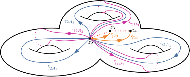
Figure 2: Integration cycles ($\tilde{\gamma}$, locally finite cycles) and branch cuts ( in red) for $T(z_{1})$, for $z_{1}\in\Sigma_{g}$, for $(g,n)=(3,4)$. Not pictured here: branch cuts for $\mathfrak{A}$- and $\mathfrak{B}$-cycle monodromies. Note that we use $A$- and $B$- to refer to the twisted $\mathfrak{A}$- and $\mathfrak{B}$-cycles.

3.1 Twisted cohomology groups of genus $g$ hypergeometric integrals

Watanabe watanabe2016twisted describes a twisted cohomology on a punctured Riemann surface of genus $g$ with $(n-1)$ punctures, $\Sigma_{g}^{*}=\Sigma_{g}-\{z_{2},z_{3},\ldots,z_{n}\}$. To do this, he introduces a multivalued function $T(z_{1})$, which factors,

$$T(z_{1})=T_{1}(z_{1})T_{2}(z_{1})\,,$$ (27)

such that $T_{1}(z_{1})$ and $T_{2}(z_{1})$ behave differently under analytic continuation. We will take the analytic continuation along paths in the fundamental group of $\Sigma_{g}^{*}$.

Let $p$ be a fixed point on $\Sigma_{g}^{*}$. The fundamental group on the punctured Riemann surface $\Sigma_{g}^{*}$ is $\pi_{1}(\Sigma_{g}^{*},p)$; it is generated by loops around the $A$- and $B$-cycles as well as loops that enclose each puncture $\{z_{j}\}_{j=2}^{n}$. We denote these loops by $\alpha_{I}$, $\beta_{I}$ and $M_{n}$, respectively. These generators satisfy a single relation:

$$\prod_{i=I}^{g}\alpha_{I}\beta_{I}\alpha_{I}^{-1}\beta_{I}^{-1}=M_{2}M_{3}\ldots M_{n}\,.$$ (28)

Then, by denoting the analytic continuation of $z_{1}$ along a loop $\delta\in\pi_{1}(\Sigma_{g}^{*})$ as $T^{\delta}(z_{1})$, we have:

$$T^{\delta}(z_{1})=\rho(\delta)T(z_{1})\,,$$ (29)

for some nonzero complex number $\rho(\delta)$. That is, we have a 1-dimensional representation for the first fundamental group

$$\rho:\pi_{1}(x)\rightarrow\mathbb{C}^{*}=\mathbb{C}\backslash\{0\}.$$ (30)

$T_{1}(z_{1})$ differs from $T_{2}(z_{1})$ in that $T_{2}(z_{1})$ has trivial monodromies under the loops $\{M_{j}\}_{j=2}^{n}$:

$$T_{2}^{M_{j}}(z_{1})=T_{2}(z_{1})\,,\,\,j=2,3,\ldots,n\,.$$ (31)

In other words, all the nontrivial of monodromies of $T(z_{1})$ for $z_{1}$ going around the other punctures is carried by $T_{1}(z_{1})$:

$$T_{1}^{M_{j}}(z_{1})=e^{2\pi is_{1j}}T_{1}(z_{1})\,,\,\,j=2,3,\ldots,n\,.$$ (32)

Combining the above equation with (24), the map $\rho$ can be made explicit

$$\rho(M_{i}) :=e^{2\pi is_{1i}}\,, \rho(\mathfrak{A}_{I}) :=e^{2\pi is_{1A_{I}}}\,, \rho(\mathfrak{B}_{I}) :=e^{2\pi is_{1B_{I}}}\,,$$ (33)

where $s_{1B_{I}}$ is fixed in (25). Note that because the target space of $\rho$ is an Abelian group (the multiplicative group of nonzero complex numbers $\mathbb{C}^{*}$), equation (28) implies

$$\rho(M_{2})\rho(M_{3})\ldots\rho(M_{n})=1\,.$$ (34)

This condition is equivalent to the momentum conservation condition in (20).

One can characterize $T_{1}(z)$ by its logarithmic differential watanabe2016twisted :

$$\text{d}_{z_{1}}\log T_{1}(z_{1})=\sum_{j=2}^{n-1}s_{1j}{\omega}(z_{1})_{z_{j},z_{n}}\,.$$ (35)

We claim that $T_{1}(z_{1})$ can be written in terms of prime functions:

$$T_{1}(z_{1})=\prod_{j=2}^{n}[E(z_{1},z_{j})]^{s_{1j}}\,.$$ (36)

This can be readily seen by using momentum conservation, and the definition of the Abelian differential of the third kind:

$$\text{d}_{z_{1}}\log T_{1}(z_{1}) =\text{d}_{z_{1}}\log\prod_{j=2}^{n}[E(z_{1},z_{j})]^{s_{1j}}=\text{d}_{z_{1}}\log\prod_{j=2}^{n-1}\left[\frac{E(z_{1},z_{j})}{E(z_{1},z_{n})}\right]^{s_{1j}}\,$$

$$=\text{d}_{z_{1}}\sum_{j=2}^{n-1}s_{1j}\log\frac{E(z_{1},z_{j})}{E(z_{1},z_{n})}=\sum_{j=2}^{n-1}s_{1j}{\omega}(z_{1})_{z_{j},z_{n}}\,.$$ (37)

Thus, after comparing with (21), we identify the multivalued function $T_{2}(z_{1})$ with the exponential of Abelian integrals:

$$T_{2}(z_{1})=\exp\left[2\pi i\sum_{I=1}^{g}s_{1A_{I}}\nu_{I}(z_{1})\right]\,.$$ (38)

The logarithmic derivative of $T_{2}(z_{1})$,

$$\text{d}_{z_{1}}\log T_{2}(z_{1})=2\pi i\sum_{I=1}^{g}s_{1A_{I}}{\omega}_{I}(z_{1})\,,$$ (39)

is also a linear combination of Abelian differentials of the first kind.

Next, we define the twisted differential, $\nabla_{\omega}:\Omega^{k}(\Sigma_{g})\rightarrow\Omega^{k+1}(\Sigma_{g})$ as:

$$\nabla_{\omega} :=\text{d}_{z_{1}}+\omega\wedge\,, \omega :=\text{d}_{z_{1}}\log T(z_{1})\,.$$ (40)

That is, given $\xi$, a $k$-form (single-valued on $\Sigma_{g}^{*}$), $\nabla_{\omega}\xi=\text{d}_{z_{1}}\xi+\text{d}_{z_{1}}\log T(z_{1})\wedge\xi$ is a $(k+1)$-form (single-valued on $\Sigma_{g}^{*}$). Since the twisted differential is nilpotent $\nabla_{\omega}^{2}=0$, we can define the $k$-th twisted de Rham cohomology group $H^{k}(\Sigma_{g}^{*},\nabla_{\omega})$:

$$H^{k}(\Sigma_{g}^{*},\nabla_{\omega})=\frac{\operatorname{Ker(\nabla_{\omega}:\Omega^{k}(\Sigma_{g}^{*})\rightarrow\Omega^{k+1}(\Sigma_{g}^{*}))}}{\operatorname{Im(\nabla_{\omega}:\Omega^{k-1}(\Sigma_{g}^{*})\rightarrow\Omega^{k}(\Sigma_{g}^{*}))}}\,.$$ (41)

By Watanabe watanabe2016twisted , we have that $H^{k}(\Sigma_{g}^{*},\nabla_{\omega})$ is nontrivial only for $k=1$. He also provides a basis of this twisted cohomology group under certain conditions.

Proposition 3.1.

Under the condition $n>\max(2,2g-1)$, the first twisted cohomology group of the genus-$g$ punctured Riemann surface $\Sigma_{g}^{*}$, $H^{1}(\Sigma_{g}^{*},\nabla_{\omega})$, is spanned by the $(2g{+}n{-}3)$-many 1-forms:

$$H^{1}(\Sigma_{g}^{*},\nabla_{\omega})={\operatorname{span}}( {\omega}_{1},{\omega}_{2},\ldots,{\omega}_{g},{\tau}_{z_{2}}(z_{1}),{\tau}_{z_{3}}(z_{1}),\ldots,{\tau}_{z_{g+1}}(z_{1}),$$

$${\omega}_{z_{2},z_{3}}(z_{1}),{\omega}_{z_{3},z_{4}}(z_{1}),\ldots,{\omega}_{z_{n-2},z_{n-1}}(z_{1}))\,\,.$$ (42)

Moreover, we have $\operatorname{dim}H^{1}(\Sigma_{g}^{*},\nabla_{\omega})=(2g+n-3)$. Therefore, the above spanning set constitutes a basis and this twisted cohomology can be spanned by the Abelian differentials of first, second and third kind where the latter two have poles at $z_{1}=z_{j}\in\{z_{2},z_{3},\ldots,z_{n}\}$.

Proof.

This is the content of (watanabe2016twisted, , theorem 4.1, example 2); what Watanabe calls the holomorphically trivial case. Nontrivially, what we call $\nabla_{\omega}$ differs from Watanabe’s twisted differential (which we call $\nabla_{\textrm{Watanabe}}$) by:

$$\nabla_{\textrm{Watanabe}}-\nabla_{\omega}=-\nabla_{z_{1}}\log T_{2}(z_{1})\,.$$ (43)

That is, the difference between the twisted differential s here and in watanabe2016twisted is a linear combination of holomorphic differentials on the (non-punctured) Riemann surface $\Sigma_{g}$. This does not change the divisor $D$ in Watanabe’s construction – holomorphic differentials do not contribute to the logarithmic singularities generated by the logarithmic derivative of the twist – and our claim follows. ∎

We are interested in these twisted cohomology groups because the genus-$g$ hypergeometric integrals $I_{\gamma}^{\varphi}(z_{i},s_{ij})$ of (21) depend on $\varphi$ only by its equivalence class in the twisted cohomology, i.e. $I_{\gamma}^{\varphi}(z_{i},s_{ij})$ is a function of $[\varphi]\in H^{1}(\Sigma_{g}^{*},\nabla_{\omega})$. This is a consequence of (26) and Stokes’ theorem. The integral $I_{\gamma}^{\varphi}(z_{i},s_{ij})$ also only depends on the equivalence class of integration contours $\gamma$ in twisted homology. This is the subject of the next section.

4 Twisted homology groups of genus-$g$ hypergeometric integrals

To set up the twisted homology, we must first define the local system $\mathcal{L}_{\boldsymbol{s}}$ associated to the twist $T(z_{1})$ where $\boldsymbol{s}=(s_{12},\dots,s_{1n},\allowbreak s_{1A_{1}},\dots,s_{1A_{g}},\allowbreak s_{1B_{1}},\dots,s_{1B_{g}})$ are parameters controlling the monodromies of the twist (33). The local system is a locally trivial line bundle whose sections are $T(z_{1})$. More plainly,

$$\mathcal{L}_{\boldsymbol{s}}=\mathbb{C}T(z_{1})=\{\text{functions }u:\nabla_{-\omega}\;u=0\}\,.$$ (44)

The local system can also be thought of as the line bundle $\mathcal{L}_{\boldsymbol{s}}=(\tilde{\Sigma}_{g}^{*}\times\mathbb{C}^{*})/\pi_{1}(\Sigma_{g}^{*})\to\Sigma_{g}^{*}$ where $\rho$ (c.f., (30)) forms a 1-dimensional representation for $\pi_{1}$ and $\tilde{\Sigma}_{g}^{*}$ is the universal cover of $\Sigma_{g}^{*}$. This viewpoint emphasizes the connection between the local system and the monodromies of the integrands.

Let $C_{m}(\Sigma_{g}^{*})$ be the space of $m$-chains on $\Sigma_{g}^{*}$. The $m$-chains $\Delta\in C_{m}(\Sigma_{g}^{*})$ with coefficients over the local system, $C_{m}(\Sigma_{g}^{*},\mathcal{L}_{\boldsymbol{s}})$, are obtained by tensoring with $T(z_{1})$:

$$\Delta\otimes T(z_{1})\in C_{m}(\Sigma_{g}^{*},\mathcal{L}_{\boldsymbol{s}})\,.$$ (45)

These are known as loaded or twisted chains. Let the twisted boundary operator $\partial_{\omega}$ be the boundary operator naturally defined for such twisted $m$-chains. Explicitly,

$$\partial_{\omega}:\ C_{m}(\Sigma_{g}^{*},\mathcal{L}_{\boldsymbol{s}}) \rightarrow C_{m-1}(\Sigma_{g}^{*},\mathcal{L}_{\boldsymbol{s}})$$

$$\partial_{\omega}:\ \Delta\otimes T(z_{1}) \mapsto\sum_{c_{i}\in\partial\Delta}c_{i}\otimes T(z_{1})|_{c_{i}}\,\,,$$ (46)

where the boundary of the $m$-chain $\Delta$ decomposes into a sum over $(m-1)$-chains $c_{i}\in C_{m-1}(\Sigma_{g}^{*})$, and $T(z_{1})|_{c_{i}}$ denotes the restriction of $T(z_{1})$ to the boundary $c_{i}$.

Since the twisted boundary operator is nilpotent ($\partial_{\omega}^{2}=0$), we can define the twisted homology groups:

$$H_{k}(\Sigma_{g}^{*},\mathcal{L}_{\boldsymbol{s}})=\frac{\operatorname{Ker}\left(\partial_{\omega}:C_{m}(\Sigma_{g}^{*},\mathcal{L}_{\boldsymbol{s}})\rightarrow C_{m-1}(\Sigma_{g}^{*},\mathcal{L}_{\boldsymbol{s}}))\right)}{\operatorname{Im}\left(\partial_{\omega}:C_{m+1}(\Sigma_{g}^{*},\mathcal{L}_{\boldsymbol{s}})\rightarrow C_{m}(\Sigma_{g}^{*},\mathcal{L}_{\boldsymbol{s}})\right)}\,.$$ (47)

Integration forms a non-degenerate pairing between the twisted homology and cohomology groups

$$I^{\varphi}_{\gamma}=[\gamma|\varphi\rangle:\ H^{1}(\Sigma_{g}^{*},\nabla_{\omega}) \times H_{1}(\Sigma_{g}^{*},\mathcal{L}_{\boldsymbol{s}})\!\!\! \rightarrow \mathbb{C}\,,$$ (48)

$$(\varphi,\gamma) \mapsto [\gamma|\varphi\rangle=\int_{\gamma}T(z_{1})\varphi\,.$$

Here, the twisted cycle simply specifies that we use the branch choice (section) $T_{\Delta}$ for the twist:

$$\int_{\gamma}T(z_{1})\varphi=\int_{\Delta\otimes T_{\Delta}}T(z_{1})\varphi=\int_{\Delta}T_{\Delta}(z_{1})\varphi\,.$$ (49)

The fact that the integration pairing between twisted homology and cohomology groups is non-degenerate is the content of twisted de Rham duality. As a consequence, the twisted homology and cohomology groups are isomorphic aomoto2011theory : this implies the only nontrivial twisted homology group is $H_{1}(\Sigma_{g}^{*},\mathcal{L}_{\boldsymbol{s}})$. Moreover, we also sometimes use the notation $H^{1}(\Sigma_{g}^{*},\mathcal{L}_{\boldsymbol{s}})$ for $H^{1}(\Sigma_{g}^{*},\nabla_{\omega})$ to emphasize that it is (de Rham) dual to the homology group $H_{1}(\Sigma_{g}^{*},\mathcal{L}_{\boldsymbol{s}})$.

A closely related homology group to $H_{1}(\Sigma_{g}^{*},\mathcal{L}_{\boldsymbol{s}})$ is the first locally finite twisted homology group, $H^{l\!f}_{1}(\Sigma_{g}^{*},\mathcal{L}_{\boldsymbol{s}})$. The 1-cycles $\tilde{\gamma}\in H^{l\!f}_{k}(\Sigma_{g}^{*},\mathcal{L}_{\boldsymbol{s}})$ are of the form:

$$\tilde{\gamma}=\sum_{i\in I}k_{i}\Delta_{i}\otimes T(z_{1})\,,$$ (50)

where the set $I$ is allowed to be infinite, but there are only finitely many $i\in I$ where the $\Delta_{i}$ intersect a compact subset of $\Sigma_{g}^{*}$. We remark that $\Sigma_{g}^{*}$ is non-compact, so representatives $[\tilde{\gamma}]\in H^{l\!f}_{1}(\Sigma_{g}^{*},\mathcal{L}_{\boldsymbol{s}})$ are generically written as infinite sums over a cover $\{U_{i}\}_{i\in I}$ for $\Sigma_{g}^{*}$. We can get some intuition by drawing such cycles $\tilde{\gamma}$, as in figure 2. Locally finite homology seems to have a complicated definition, but the corresponding integration contours are easy to draw: it just happens that the start and end points of these contours are points that have been removed from the Riemann surface!

The singular and locally finite twisted homology groups are isomorphic. One direction of this isomorphism is via the natural inclusion:

$$i:H_{1}(\Sigma_{g}^{*},\mathcal{L}_{\boldsymbol{s}})\xrightarrow{\sim}H^{l\!f}_{1}(\Sigma_{g}^{*},\mathcal{L}_{\boldsymbol{s}})\,.$$ (51)

The inverse of the above map is called the regularization isomorphism

$$\mathrm{reg}:H^{l\!f}_{1}(\Sigma_{g}^{*},\mathcal{L}_{\boldsymbol{s}})\xrightarrow{\sim}H_{1}(\Sigma_{g}^{*},\mathcal{L}_{\boldsymbol{s}})\,.$$ (52)

and is detailed in section 4.2.

4.1 Generators of twisted homology

An advantage of twisted homology is that we can work with integrands that are multivalued on $\Sigma_{g}^{*}$ without needing to introduce its universal cover $\tilde{\Sigma}_{g}^{*}$. In order to do this, we need to specify branch choices and branch cuts of $T(z_{1})$.

The twist $T(z_{1})$ has short and long branch cuts. The short branch cuts join $z_{j}$ to $z_{j+1}$, for $j=2,3,\ldots,n-1$ (red dashed lines in figure 2). The long branch cuts are homologous to $\mathfrak{A}$- and $\mathfrak{B}$- cycles. For ease of description, let’s assume that the punctures $z_{2},z_{3},\ldots,z_{n}$ are close to each other and arranged such that, in a local chart, $0<\arg(z_{j+1}-z_{j})<\pi/2$. Following ghazouani2016moduli , we say that punctures like these are in a nice position.

The locally finite cycles $\tilde{\gamma}_{2j}$ connecting $z_{2}$ to $z_{j}$ start and end below the short branch cut. These are shown in orange in figures 2. The locally finite cycles $\tilde{\gamma}_{2A_{I}}$ (respectively, $\tilde{\gamma}_{2B_{J}}$) start and end at the puncture $z_{2}$ and are homologous to the $\mathfrak{A}_{I}$-cycles (respectively $\mathfrak{B}_{J}$-cycles).

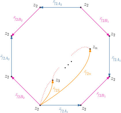
Figure 3: Structure of a genus two surface as the $z_{1}$-space cut open to an octagon, i.e. by its canonical dissection. This is the integration domain for genus-two hypergeometric integrals with $n$ punctures. The red dotted lines show our branch cut residing inside this octagon. For any genus $g\geq 1$, we require this branch cut to reside inside the $4g$-gon.

The relative positions and orientations of the locally finite cycles boils down to the following: if we cut the surface $\Sigma_{g}$ along the $\tilde{\gamma}_{2A_{I}}$ and $\tilde{\gamma}_{2B_{J}}$ cycles, we obtain a canonical dissection of the surface (see e.g. (hejhal1972theta, , figure 9)). Once cut along these cycles, $\Sigma_{g}$ makes a $4g$-gon where the puncture $z_{2}$ is repeated at each vertex. Moreover, the short branch cuts extend into the interior of this $4g$-gon. See figure 3 for an example at genus two.

It turns out that the set of cycles pictured in figure 3 are over-complete and there is one linear relation among them. To see this, let $A$ be the interior of the $4g$-gon, as a loaded $2$-simplex. Its twisted boundary is given by:

$$\partial_{\omega}A =\sum_{I=1}^{g}\left(1-e^{2\pi is_{1B_{I}}}\right)\tilde{\gamma}_{2A_{I}}+\sum_{I=1}^{g}\left(e^{2\pi is_{1A_{I}}}-1\right)\tilde{\gamma}_{2B_{I}}$$

$$\phantom{=}+\sum_{j=2}^{n}e^{-2\pi i(s_{12}+s_{13}+\ldots+s_{1j})}\left(e^{2\pi is_{1j}}-1\right)\tilde{\gamma}_{2j}\,\,.$$ (53)

The above implies the following linear relation in twisted homology:

$$0 =\sum_{I=1}^{g}\left(1-e^{2\pi is_{1B_{I}}}\right)[\tilde{\gamma}_{2A_{I}}]+\sum_{I=1}^{g}\left(e^{2\pi is_{1A_{I}}}-1\right)[\tilde{\gamma}_{2B_{I}}]$$

$$\phantom{=}+\sum_{j=2}^{n}e^{-2\pi i(s_{12}+s_{13}+\ldots+s_{1j})}\left(e^{2\pi is_{1j}}-1\right)[\tilde{\gamma}_{2j}]\,\,,$$ (54)

for $[\tilde{\gamma}_{a}]\in H^{l\!f}_{1}(\Sigma_{g}^{*},\mathcal{L}_{\boldsymbol{s}})$. In the physics literature, relations like the above are known as monodromy relations Casali:2019ihm ; Casali:2020knc . Due to the monodromy relations, we note that the twisted homology group $H^{l\!f}_{1}(\Sigma_{g}^{*},\mathcal{L}_{\boldsymbol{s}})$ is spanned by these $(2g+n-2)$ locally finite cycles $\tilde{\gamma}_{a}$ subject to one linear relation, given by (4.1).

Claim 4.1.

The twisted homology group $H^{l\!f}_{1}(\Sigma_{g}^{*},\mathcal{L}_{\boldsymbol{s}})$ is spanned by locally finite cycles:

$$H^{l\!f}_{1}(\Sigma_{g}^{*},\mathcal{L}_{\boldsymbol{s}})=\mathrm{span}\{\tilde{\gamma}_{2A_{1}},\tilde{\gamma}_{2B_{1}},\tilde{\gamma}_{2A_{2}},\tilde{\gamma}_{2B_{2}},\ldots,\tilde{\gamma}_{2A_{g}},\tilde{\gamma}_{2B_{g}},\tilde{\gamma}_{23},\tilde{\gamma}_{24},\ldots,\tilde{\gamma}_{2n}\}\,.$$ (55)

subject to the single linear relation (4.1).

We will verify this statement analytically in section 4.3 by studying the determinants of specific matrices whose entries are homology intersection numbers. Additionally, we verify this statement by replacing $\gamma\to\int_{\gamma}T(z_{1})\,\omega_{I}$ in (4.1) and numerically evaluating the resulting integrals. See the ancillary files for the numerical implementation.

4.2 Regularization of cycles

The homology intersection numbers are an integral piece of the double copy. In order to compute them, we needed a basis of the twisted homology group $H_{1}(\Sigma_{g}^{*},\mathcal{L}_{\boldsymbol{s}})$ consisting of regulated cycles. To do this, we need to specify a cellular decomposition of $\Sigma_{g}^{*}$ by specifying certain points and $1$-chains.

Let $P_{0},P_{1},\ldots,P_{4g-1}$ be points centered around the puncture $z_{2}$, at a small distance $\epsilon$ from $z_{2}$, numbered counterclockwise. Also put $P_{0}$ below the short branch cut connecting $z_{2}$ to $z_{3}$ and $P_{1}$ above this short branch cut. We will also need points $Q_{j}$, located at a small distance $\epsilon$ from $z_{j}$ below the short branch cut, for $j=3,4,\ldots,n$. See figure 4 for an example of the placements of these points on a genus-$2$ surface.

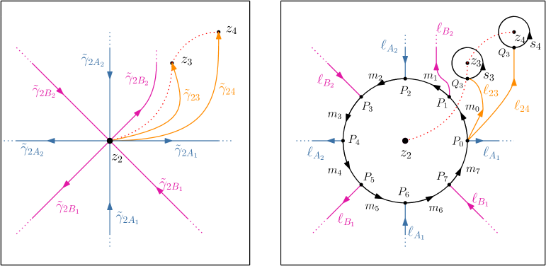
Figure 4: A local picture of a punctured genus-two surface $\Sigma_{2}^{*}$. The contours $\tilde{\gamma}_{2A_{\bullet}}$,$\tilde{\gamma}_{2B_{\bullet}}$,$\ell_{A_{\bullet}}$,$\ell_{B_{\bullet}}$ go around the corresponding homology cycles, and intersect outside this local picture. Left: Locally finite, spanning set of cycles. Right: regulated cycles. For concreteness we use $n=4$ here. Note that the regularization procedure happens only around the punctures, and thus such a local picture like this suffices.

With these points in place, let $m_{j}$ be $1$-chains consisting of circular arcs centered around $z_{2}$ going counterclockwise from $P_{j}$ to $P_{j+1}$, except for $m_{4g-1}$ which goes from $P_{4g-1}$ to $P_{0}$. Let $s_{j}$ be the circular arc centered around $z_{j}$, starting and ending at $Q_{j}$, for $j=3,4,\ldots,n$, and $\ell_{2j}$ be the $1$-chains going from $P_{0}$ to $Q_{j}$. Furthermore, we define the long $1$-chains $\ell_{A_{J}}$ ($\ell_{B_{J}}$) that start at $P_{4g-4J+4}$ ($P_{4g-4J+1}$) and end at $P_{4g-4J+2}$ ($P_{4g-4J+3}$). Here, all all subindices are taken modulo $4g$ and none of the long $1$-chains intersect each other. Lastly, let $\tilde{A}$ be the $2$-chain given by the connected exterior of the circles surrounding the punctures $z_{2},z_{3},\ldots,z_{n}$. The disjoint union of the points $\{P_{\bullet},Q_{\bullet}\}$, $1$-chains $\{\ell_{\bullet},m_{\bullet}\}$, and the $2$-chain $\tilde{A}$, give the cellular decomposition of the punctured genus-$g$ Riemann surface $\Sigma_{g}^{*}$. Thus, we can use these chains to write down bases for the twisted homology group $H_{1}(\Sigma_{g}^{*},\mathcal{L}_{\boldsymbol{s}})$.

To build the regularized cycles, it is useful to record the twisted boundaries of some $1$-chains:

$$\partial_{\omega}s_{j} =\left(e^{2\pi is_{1j}}-1\right)Q_{j}\,, j=3\ldots,n\,,$$

$$\partial_{\omega}m_{0} =e^{2\pi is_{12}}P_{1}-P_{0}\,,$$

$$\partial_{\omega}m_{j} =P_{j+1}-P_{j}\,, j\neq 0\,,$$

$$\partial_{\omega}(m_{0}+e^{2\pi is_{12}}\sum_{j=1}^{4g}m_{j}) =(e^{2\pi is_{12}}-1)P_{0}\,,$$

$$\partial_{\omega}\ell_{A_{J}} =e^{2\pi is_{1A_{J}}}P_{4g-4J+2}-P_{4g-4J+4}\,, J=1,2,\ldots,g\,,$$

$$\partial_{\omega}\ell_{B_{J}} =e^{2\pi is_{1B_{J}}}P_{4g-4J+3}-P_{4g-4J+1}\,, J=1,2,\ldots,g\,,$$ (56)

where the always take the subindex of $P_{i}$ to be modulo $4g$.

Theorem 4.2.

A spanning set of regularized cycles $\gamma_{a}\in H_{1}(\Sigma_{g}^{*},\mathcal{L}_{\boldsymbol{s}})$ is given by:

$$[\gamma_{2j}]=\mathrm{reg}[\tilde{\gamma}_{2j}] =\frac{m_{0}+e^{2\pi is_{12}}\sum_{k=1}^{4g-1}m_{k}}{e^{2\pi is_{12}}-1}+\ell_{2j}-\frac{s_{j}}{e^{2\pi is_{1j}}-1}\,, j=3,\ldots,n\,,$$

$$[\gamma_{2A_{1}}]=\mathrm{reg}[\tilde{\gamma}_{2A_{1}}] =\frac{m_{0}+e^{2\pi is_{12}}\sum_{k=1}^{4g-1}m_{k}}{e^{2\pi is_{12}}-1}$$

$$\phantom{=}+\ell_{A_{1}}$$

$$\phantom{=}-e^{2\pi is_{1A_{1}}}\frac{m_{0}+m_{4g-1}+m_{4g-2}+e^{2\pi is_{12}}\sum_{k=1}^{4g-3}m_{k}}{e^{2\pi is_{12}}-1}\,,$$

$$[\gamma_{2A_{J}}]=\mathrm{reg}[\tilde{\gamma}_{2A_{J}}] =\frac{m_{0}+\sum_{k=4g-4J+4}^{4g-1}m_{k}+e^{2\pi is_{12}}\sum_{k=1}^{4g-4J+3}m_{k}}{e^{2\pi is_{12}}-1}$$

$$\phantom{=}+\ell_{A_{J}}$$

$$\phantom{=}-e^{2\pi is_{1A_{J}}}\frac{m_{0}+\sum_{k=4g-4J+2}^{4g-1}m_{k}+e^{2\pi is_{12}}\sum_{k=1}^{4g-4J+1}m_{k}}{e^{2\pi is_{12}}-1}\,,\, J=2,\ldots,g\,,$$

$$[\gamma_{2B_{g}}]=\mathrm{reg}[\tilde{\gamma}_{2B_{g}}] =\frac{\sum_{k=0}^{4g-1}m_{k}}{e^{2\pi is_{12}}-1}$$

$$\phantom{=}+\ell_{B_{g}}$$

$$\phantom{=}-e^{2\pi is_{1B_{g}}}\frac{m_{0}+\sum_{k=3}^{4g-1}m_{k}+e^{2\pi is_{12}}(m_{1}+m_{2})}{e^{2\pi is_{12}}-1}\,,$$ (57)

$$[\gamma_{2B_{J}}]=\mathrm{reg}[\tilde{\gamma}_{2B_{J}}] =\frac{m_{0}+\sum_{k=4g-4J+1}^{4g-1}m_{k}+e^{2\pi is_{12}}\sum_{k=1}^{4g-4J}m_{k}}{e^{2\pi is_{12}}-1}$$

$$\phantom{=}+\ell_{B_{J}}$$

$$\phantom{=}-e^{2\pi is_{1B_{J}}}\frac{m_{0}+\sum_{k=4g-4J+3}^{4g-1}m_{k}+e^{2\pi is_{12}}\sum_{k=1}^{4g-4J+2}m_{k}}{e^{2\pi is_{12}}-1}\,, J=1,\ldots,g-1\,.$$ (58)

These cycles satisfy one linear relation and any collection of $2g+n-3$ of these cycles form a basis of the twisted homology for generic choices of $\{s_{1j},s_{1A_{J}},s_{1B_{J}}\}v$, $j=2,\ldots,n$, $J=1,\ldots,g$.

Proof.

Using (4.2), one can explicitly verify that these are twisted cycles: $\partial_{\omega}\gamma_{\bullet}=0$. Alternatively, one can show these regularized cycles are proportional to Pochhammer contours which are obviously closed contours.

Moreover, any collection of $2g+n-3$ of these cycles form a basis. This follows from the fact that such a collection of cycles has cardinality equal to the dimension of the twisted homology group and that the determinant of the corresponding $(2g+n-3)\times(2g+n-3)$ intersection matrix is non-vanishing. We demonstrate that the determinant of the intersection matrix associated to the set $\{\gamma_{2A_{J}},\gamma_{2B_{J}},\gamma_{2j}\}_{\begin{subarray}{c}\hskip-10.0ptJ=1,\dots,g\\ j=3,\dots,n-1\end{subarray}}$ is non-vanishing in equation (79). ∎

In (4.2) we have included the cycles $\gamma_{2A_{1}}$ and $\gamma_{2B_{g}}$ as separate cases for convenience of the reader. Moreover, each cycle $\gamma_{2A_{J}}$ and $\gamma_{2B_{J}}$ is written in three lines, where the terms in the first and third lines have simple twisted boundaries. This way, the reader can readily verify that these cycles have no twisted boundary.

Corollary 4.3.

The regularized cycles also satisfy the linear relation (4.1):

$$0 =\sum_{I=1}^{g}\left(1-e^{2\pi is_{1B_{I}}}\right)[\gamma_{2A_{I}}]+\sum_{I=1}^{g}\left(e^{2\pi is_{1A_{I}}}-1\right)[{\gamma}_{2B_{I}}]$$

$$\phantom{=}+\sum_{j=2}^{n}e^{-2\pi i(s_{12}+s_{13}+\ldots+s_{1j})}\left(e^{2\pi is_{1j}}-1\right)[{\gamma}_{2j}]\,\,.$$ (59)

With these regularized cycles, we can compute the intersection pairing in twisted homology.

4.3 Homology intersection numbers

Let $\check{\mathcal{L}}_{\boldsymbol{s}}$ be the local system coming from the multivaluedness of $T(z_{1})^{-1}$. We call this the dual local system of $\mathcal{L}_{\boldsymbol{s}}$. It is related to $\mathcal{L}_{\boldsymbol{s}}$ by changing the sign of all $s_{1j}$’s:

$$\check{\mathcal{L}}_{\boldsymbol{s}}:=[\mathcal{L}_{\boldsymbol{s}}]^{\vee}=\mathcal{L}_{-\boldsymbol{s}}\,,$$ (60)

where $(\bullet)^{\vee}:=\bullet|_{s_{ij}\to-s_{ij}}$. We can define an intersection pairing $[\bullet|\bullet]$ between the twisted homology groups $H_{1}(\Sigma_{g}^{*},\mathcal{L}_{\boldsymbol{s}})$ and $H_{1}(\Sigma_{g}^{*},\mathcal{L}_{-\boldsymbol{s}})$:

$$[\bullet|\bullet]:H_{1}(\Sigma_{g}^{*},\mathcal{L}_{\boldsymbol{s}})\,\times\,H_{1}(\Sigma_{g}^{*},\mathcal{L}_{-\boldsymbol{s}})\rightarrow\mathbb{C}\,,$$ (61)

given by

$$[\gamma\otimes T_{\gamma}(z_{1})|\check{\gamma}\otimes T_{\check{\gamma}}(z_{1})^{-1}]\mapsto\sum_{x\in\gamma\cap\check{\gamma}}\,\left(T_{\gamma}(z_{1})T_{\check{\gamma}}(z_{1})^{-1}|_{x}\right)[\gamma|\check{\gamma}]^{\textrm{top}}_{x},$$ (62)

where the cycles $\gamma$ and $\check{\gamma}$ intersect a finite number of times, $T_{\gamma}(z_{1})$ refers to the local determination of $T(z_{1})$ on the loaded cycle $\gamma$, and $T_{\gamma}(z_{1})T_{\check{\gamma}}(z_{1})^{-1}|_{x}$ evaluates to some phase for any given $x$. The topological intersection index $[\bullet|\bullet]_{x}^{\textrm{top}}$ evaluates to $+1$ or $-1$ depending on the relative orientation of $\gamma$ and $\check{\gamma}$. Following the conventions of Mizera:2017cqs ; mimachi2002intersection we use:

$$\begin{gathered}\includegraphics[scale={0.5}]{figs/topological_intersection_numbers.png}\end{gathered}\,.$$ (64)

Remark 4.4.

If $\check{\gamma}\in H_{1}(\Sigma_{g}^{*},\mathcal{L}_{-\boldsymbol{s}})$ and ${\gamma}\in H_{1}(\Sigma_{g}^{*},\mathcal{L}_{\boldsymbol{s}})$ are regularized cycles, i.e.

$$\check{\gamma} =\mathrm{reg}\,{\check{\gamma}}\,, {\gamma} =\mathrm{reg}\,{\gamma}\,,$$ (65)

for $\tilde{\check{\gamma}}\in H^{l\!f}_{1}(\Sigma_{g}^{*},\mathcal{L}_{-\boldsymbol{s}})$ and $\tilde{\gamma}\in H^{l\!f}_{1}(\Sigma_{g}^{*},\mathcal{L}_{\boldsymbol{s}})$, the homology intersection numbers $[\gamma|\check{\gamma}]$ can be computed by regulating at least one locally finite cycle:

$$[\gamma|\check{\gamma}]=[\tilde{\gamma}|\check{\gamma}]=[\gamma|\tilde{\check{\gamma}}]\,.$$ (66)

That is, we are free to use one locally finite cycle when computing such intersection numbers, and the answer coincides with the result obtained from regularizing both locally finite cycles.

Conveniently, the homology intersection number behaves nicely with respect to the dualizing operation $(\bullet)^{\vee}$ via $\bullet\mapsto\bullet|_{s_{ij}\to-s_{ij}}$. This map is an involution on $\mathbb{C}(\exp(2\pi is_{1j}))$ and maps between the twisted homology groups

$$()^{\vee}: H_{1}(\Sigma_{g}^{*},\mathcal{L}_{\boldsymbol{s}})\rightarrow H_{1}(\Sigma_{g}^{*},\mathcal{L}_{-\boldsymbol{s}})\,,$$

$$()^{\vee}: H_{1}(\Sigma_{g}^{*},{\mathcal{L}}_{-\boldsymbol{s}})\rightarrow H_{1}(\Sigma_{g}^{*},\mathcal{L}_{\boldsymbol{s}})\,.$$ (67)

For example, if $\gamma=\Delta\otimes T_{\Delta}\in H_{1}(\Sigma_{g}^{*},\mathcal{L}_{\boldsymbol{s}})$ is a twisted cycle. Its image under $()^{\vee}$ is $\check{\gamma}=\Delta\otimes T_{\Delta}^{-1}\in H_{1}(\Sigma_{g}^{*},{\mathcal{L}}_{-\boldsymbol{s}})$; changing the signs of $s_{1j}$ simply changes the loading $T_{\Delta}(z_{1})\to T_{\Delta}(z_{1})^{-1}$. Then, the homology intersection number satisfies:

$$[\gamma_{A}|\check{\gamma}_{B}]^{\vee}=-[\check{\gamma}^{\vee}_{B}|\gamma^{\vee}_{A}]=-[\gamma_{B}|\check{\gamma}_{A}]\,,$$ (68)

where the intersection number is valued in $\mathbb{C}(\exp(2\pi is_{1j}))$. This property is convenient because it reduces the number of homology intersection numbers we need to compute.

The homology intersection numbers among the regularized cycles of (4.2) are given by:

$$[\gamma_{2j}|\check{\gamma}_{2k}]=\begin{cases}-\dfrac{e^{2\pi is_{12}}}{e^{2\pi is_{12}}-1}\,,&j<k\vskip 5.0pt\\ -\dfrac{e^{2\pi i(s_{12}+s_{1j})}-1}{(e^{2\pi is_{12}}-1)(e^{2\pi is_{1j}}-1)}\,,&j=k\vskip 5.0pt\\ -\dfrac{1}{e^{2\pi is_{12}}-1}\,,&j>k\end{cases}$$ (69)

$$[\gamma_{2A_{I}}|\check{\gamma}_{2k}] =-\dfrac{1-e^{2\pi is_{1A_{I}}}}{e^{2\pi is_{12}}-1}\,,$$ (70)

$$[\gamma_{2B_{I}}|\check{\gamma}_{2k}] =-\dfrac{1-e^{2\pi is_{1B_{I}}}}{e^{2\pi is_{12}}-1}\,.$$ (71)

$$[\gamma_{2A_{I}}|\check{\gamma}_{2A_{J}}]=\begin{cases}\dfrac{e^{2\pi is_{12}}(1-e^{2\pi is_{1A_{I}}})(1-e^{-2\pi is_{1A_{J}}})}{e^{2\pi is_{12}}-1}\,,&I<J\vskip 5.0pt\\ \dfrac{(e^{2\pi is_{1A_{I}}}-1)(e^{2\pi is_{1A_{I}}}-e^{2\pi is_{12}})}{(e^{2\pi is_{12}}-1)e^{2\pi is_{1A_{I}}}}\,,&I=J\vskip 5.0pt\\ \dfrac{(1-e^{-2\pi is_{1A_{I}}})(1-e^{2\pi is_{1A_{J}}})}{e^{2\pi is_{12}}-1}\,,&I>J\end{cases}$$ (72)

$$[\gamma_{2B_{I}}|\check{\gamma}_{2B_{J}}]=\begin{cases}\dfrac{e^{2\pi is_{12}}(1-e^{2\pi is_{1B_{I}}})(1-e^{-2\pi is_{1B_{J}}})}{e^{2\pi is_{12}}-1}\,,&I<J\vskip 5.0pt\\ \dfrac{(e^{-2\pi is_{1B_{I}}}-1)(e^{-2\pi is_{1B_{I}}}-e^{2\pi is_{12}})}{(e^{2\pi is_{12}}-1)e^{-2\pi is_{1B_{I}}}}\,,&I=J\vskip 5.0pt\\ \dfrac{(1-e^{-2\pi is_{1B_{I}}})(1-e^{2\pi is_{1B_{J}}})}{e^{2\pi is_{12}}-1}\,,&I>J\end{cases}$$ (73)

$$[\gamma_{2A_{I}}|\check{\gamma}_{2B_{J}}]=\begin{cases}\frac{e^{2\pi is_{12}}(1-e^{2\pi is_{1A_{I}}})(1-e^{-2\pi is_{1B_{J}}})}{e^{2\pi is_{12}}-1}\,,&I<J\vskip 5.0pt\\ -\frac{e^{2\pi is_{12}}-e^{2\pi i(s_{1A_{I}}+s_{12})}-e^{2\pi i(s_{12}-s_{1B_{I}})}+e^{2\pi i(s_{1A_{I}}-s_{1B_{I}})}}{e^{2\pi is_{12}}-1}\,,&I=J\vskip 5.0pt\\ \frac{(1-e^{-2\pi is_{1A_{I}}})(1-e^{2\pi is_{1B_{J}}})}{e^{2\pi is_{12}}-1}\,,&I>J\end{cases}$$ (74)

$$[\gamma_{2B_{I}}|\check{\gamma}_{2A_{J}}]=\begin{cases}\frac{e^{2\pi is_{12}}(1-e^{2\pi is_{1B_{I}}})(1-e^{-2\pi is_{1A_{J}}})}{e^{2\pi is_{12}}-1}\,,&I<J\vskip 5.0pt\\ -\frac{1-e^{2\pi is_{1B_{I}}}-e^{-2\pi is_{1A_{I}}}+e^{2\pi i(-s_{1A_{I}}+s_{12}+s_{1B_{I}})}}{e^{2\pi is_{12}}-1}\,,&I=J\vskip 5.0pt\\ \frac{(1-e^{-2\pi is_{1B_{I}}})(1-e^{2\pi is_{1A_{J}}})}{e^{2\pi is_{12}}-1}\,,&I>J\end{cases}$$ (75)

We include the computation of these intersection numbers in appendix A.

We will make use of homology intersection numbers to compute certain cohomology intersection numbers via twisted Riemann bilinear relations. However, we first need to be certain that we have a basis of twisted homology.

As discussed earlier, the dimension of the twisted homology group $H_{1}(\Sigma_{g}^{*},\mathcal{L}_{\boldsymbol{s}})$ is the same as the twisted cohomology group $H^{1}(\Sigma_{g}^{*},\nabla_{\omega})$, which was computed by Watanabe:

$$\dim H_{1}(\Sigma_{g}^{*},\mathcal{L}_{\boldsymbol{s}})=H^{1}(\Sigma_{g}^{*},\nabla_{\omega})=2g+n-3\,.$$ (76)

We have constructed a set of $(2g+n-2)$ twisted cycles $\{\gamma_{2a}\}_{a=3,4,\ldots,n,A_{1},B_{1},\ldots,A_{g},B_{g}}\subset H_{1}(\Sigma_{g}^{*},\mathcal{L}_{\boldsymbol{s}})$ that are subject to the linear relation 4.3. We would like to show that 4.3 is the only linear relation these cycles satisfy. Then, any subset of cycles with cardinality $2g+n-3$ is a basis of the twisted homology.

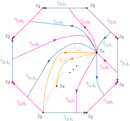
Figure 5: A set of locally finite twisted cycles, shown in the canonical dissection of figure 3. These twisted cycles are constructed such that the intersection numbers of these with the cycles $\tilde{\gamma}_{2\bullet}$ are simple to compute. Now the cycles $\tilde{\gamma}_{nj}$ start at puncture $z_{n}$ and go to puncture $j$, above the branch cut (dotted red line). The cycle $\tilde{\gamma}_{nB_{1}}$ goes from $z_{2}$ to $z_{2}$, is homologous to a $\mathfrak{B}_{1}$-cycle, and starts right below the branch cut. The orientation of the other $\tilde{\gamma}_{nA_{\bullet}}$ and $\tilde{\gamma}_{nB_{\bullet}}$ follows the order depicted here, according to the edges of the $4g$-gon.

To show that there is only one linear relation among these cycles, we could look at the determinants of certain matrices whose elements are intersection numbers that we have already computed. However, it turns out that it’s more convenient to build another set of (locally finite) twisted cycles

$$\{\check{\gamma}_{na}\}_{a=3,4,\ldots,n-1,A_{1},B_{1},\ldots,A_{g},B_{g}}\in H^{l\!f}_{1}(\Sigma_{g}^{*},\mathcal{L}_{-\boldsymbol{s}})\,,$$ (77)

see figure 5. Then, the homology intersection numbers $[\gamma_{2a}|\check{\gamma}_{nb}]$ are remarkably simple; most of them vanish. In fact, let $\mathbf{H}^{(2,n)}$ be the $(2g+n-3)\times(2g+n-3)$ matrix whose components $H^{(2,n)}_{a,b}$ are the intersection numbers:

$$H^{(2,n)}_{a,b}=[\gamma_{2a}|\check{\gamma}_{nb}]\,,\qquad a \in\{3,4,\ldots,n-1,A_{1},B_{1},A_{2},B_{2},\ldots,A_{g},B_{g}\}$$

$$b \in\{3,4,\ldots,n-1,B_{1},A_{1},B_{2},A_{2},\ldots,B_{g},A_{g}\}\,,$$ (78)

where the indices are listed in order. Then $\mathbf{H}^{(2,n)}_{a,b}$ is a diagonal matrix whose determinant is given by:

$$\det\mathbf{H}^{(2,n)}_{a,b}=\left[\prod_{j=3}^{n-1}\dfrac{e^{2\pi i(s_{12}+\ldots+s_{1j})}}{e^{2\pi is_{1j}}-1}\right]\times\left[\prod_{J=1}^{g}{e^{2\pi i(s_{1A_{J}}-s_{1B_{J}})}}\right]\times\left[e^{2g\pi is_{1n}}\right]\,.$$ (79)

In (79), the term in the first square bracket comes from the intersection numbers among the cycles between different punctures, and the last 2 square brackets contain the contribution of the cycles $[\gamma_{2A_{J}}]$, $[\gamma_{2B_{J}}]$, $[\check{\gamma}_{nA_{J}}]$, $[\check{\gamma}_{nB_{J}}]$, for $J=1,2,\ldots,g$. Note that (following the conventions of Goto2022 ) $\gamma_{2B_{J}}$ carries an extra phase $e^{2\pi is_{1n}}$ compared to $\gamma_{2A_{J}}$, which yields the last factor above.

In particular, we note that the determinant being non-singular in (79) is a sufficient condition for both of the sets of twisted cycles appearing in the matrix $\mathbf{H}^{(2,n)}$ to be $\mathbb{C}(e^{2\pi is_{1\bullet}})-$linearly independent:

$$s_{1j}\not\in\mathbb{Z}\,,\textrm{for }j=3,\ldots,n-1\,.$$ (80)

But we have already assumed that

$$s_{1j}\not\in\mathbb{Z}\,,\textrm{for }j=2,\ldots,n\,,$$ (81)

when writing down the regularized cycles in (4.2). Therefore, under these previous assumptions the sets of twisted cycles appearing in the matrix $\mathbf{H}^{(2,n)}$ are bases in twisted homology.

In practice, we will make use of the matrix of homology intersection numbers $\mathbf{H}^{(2,2)}$, with components ${H}^{(2,2)}_{ab}$ given by:

$$H^{(2,2)}_{a,b}= [\gamma_{2a}|\check{\gamma}_{2b}]\,, a,b\in\{3,4,\ldots,n-1,A_{1},B_{1},A_{2},B_{2},\ldots,A_{g},B_{g}\}.$$ (82)

Because the set of cycles $[\gamma_{2a}]$, $a\in\{3,4,\ldots,n-1,A_{1},B_{1},A_{2},B_{2},\ldots,A_{g},B_{g}\}$ is a basis of twisted homology, the matrix $\mathbf{H}^{(2,2)}$ is invertible. We denote the components of the inverse matrix ${[\mathbf{H}^{(2,2)}}]^{-1}$ raised indices $H_{(2,2)}^{ab}$. That is,

$$\sum_{b=3,4,\ldots,n-1,A_{1},B_{1},\ldots,A_{g},B_{g}}H^{(2,2)}_{a,b}H_{(2,2)}^{b,c}=\delta_{a}^{c}\,,$$ (83)

where $\delta_{a}^{c}$ is a Kronecker delta (i.e. the components of the identity matrix).

5 Cohomology intersection numbers and double copy relations

In this section, we introduce cohomology intersection numbers – another ingredient in the double copy. To define the cohomology intersection number, we need to introduce the dual twisted cohomology group

$$\big(H^{1}(\Sigma_{g}^{*},\nabla_{\omega})\big)^{\vee}=H^{1}(\Sigma_{g}^{*},\nabla_{-\omega})\,,$$ (84)

where, as before, the map $()^{\vee}$ sends $s_{1j}\to-s_{1j}$. Consequently, the dual twist and dual connection are simply related to their non-dual counterparts

$$\big(T(z_{1})\big)^{\vee} =T(z_{1})^{-1}\,, (\omega)^{\vee} =-\omega\,.$$ (85)

The map $()^{\vee}$ also maps cohomology classes $[\varphi]$ to dual cohomology classes $[\check{\varphi}]$

$$\check{\varphi}=(\varphi)^{\vee}=\varphi|_{s_{1j}\mapsto-s_{1j}}\,.$$ (86)

In particular, $\check{\varphi}$ is equal to $\varphi$ whenever $\varphi$ does not explicitly depend on $s_{1j}$.

Clearly, dual cohomology representatives $\check{\varphi}\in H^{1}(\Sigma_{g}^{*},\nabla_{-\omega})$ pair (via integration) with dual cycles $\check{\gamma}\in H_{1}(\Sigma_{g}^{*},\mathcal{L}_{-\boldsymbol{s}})$ to form dual genus-$g$ hypergeometric integrals:

$$I^{\check{\varphi}}_{\check{\gamma}}(z_{i},s_{ij})=\int_{\check{\gamma}}T(z_{1})^{-1}{\check{\varphi}}(z_{1})=I^{\varphi}_{\gamma}(z_{i},-s_{ij})=\left(I^{\varphi}_{\gamma}(z_{i},s_{ij})\right)^{\vee}\,.$$ (87)

Moreover, as displayed above, these integrals are simply related to those introduced in section 3.

The cohomology intersection pairing is constructed in a analogously to the homology intersection pairing: by regularizing one of the cocycles. To do this, we note that the twisted de Rham cohomology is isomorphic to the compactly supported cohomology aomoto2011theory

$$H^{1}(\Sigma^{*}_{g},\nabla_{\pm\omega})\simeq H^{1}_{c}(\Sigma^{*}_{g},\nabla_{\pm\omega})\,.$$ (88)

Similar to the twisted homology there is a natural inclusion map

$$i:H^{1}(\Sigma^{*}_{g},\nabla_{\pm\omega})\xrightarrow{\sim}H^{1}_{c}(\Sigma^{*}_{g},\nabla_{\pm\omega})\,,$$ (89)

as well as an inverse called regularization:

$$\mathrm{reg}:H^{1}_{c}(\Sigma^{*}_{g},\nabla_{\pm\omega})\xrightarrow{\sim}H^{1}(\Sigma^{*}_{g},\nabla_{\pm\omega})\,.$$ (90)

Then, the cohomology intersection number is defined to be cho1995 :

$$\langle\bullet|\bullet\rangle:H^{1}(\Sigma_{g}^{*},\nabla_{-\omega})\times H^{1}(\Sigma_{g}^{*},\nabla_{\omega}) \!\!\!\rightarrow\mathbb{C}$$ (91)

$$\langle\bullet|\bullet\rangle:\qquad\qquad\quad(\check{\varphi}_{k},\varphi_{l}) \!\!\!\mapsto\langle\check{\varphi}_{k}|\varphi_{l}\rangle=-\int_{\Sigma_{g}^{*}}\mathrm{reg}[\check{\varphi}_{k}]\wedge\varphi_{l}\,,$$

where it only depends on the cohomology class of $\check{\varphi}_{k}$ and $\varphi_{l}$. The defining integral is also convergent since $\mathrm{reg}[\check{\varphi}_{k}]$ has compact support away from all singularities. Note that like the homology intersection number, one is free to regulate either $\check{\varphi}$ or $\varphi$. For our purposes, we require a generalization of the above intersection number (detailed in the next section). This generalization does not require spelling out the details of the regularization map which are not presented here (the interested reader can consult aomoto2011theory ).

We remark that the cohomology intersection number $\langle\check{\varphi}_{k}|\varphi_{l}\rangle$ is non-zero if and only if there is a $z^{*}\in\Sigma_{g}$ such that $\mathrm{ord}_{z_{1}=z*}^{\mathrm{pole}}(\check{\varphi}_{k})+\mathrm{ord}_{z_{1}=z*}^{\mathrm{pole}}({\varphi}_{l})-\mathrm{ord}_{z_{1}=z*}^{\mathrm{zero}}(\check{\varphi}_{k})-\mathrm{ord}_{z_{1}=z*}^{\mathrm{zero}}({\varphi}_{l})-1>0\,,$ Therefore, since the holomorphic differentials $\omega_{I}$ are free from poles and zeros, the intersection number vanishes

$$\langle\check{\omega}_{J}|\omega_{I}\rangle=0\qquad\forall\qquad I,J\in\{1,\dots,g\}\,.$$ (92)

We will soon see how $\langle\check{\omega}_{J}|\omega_{I}\rangle=0$ leads to quadratic relations that the integrals $I^{\varphi}_{\gamma}(z_{1},s_{1j})$ and $I^{\varphi}_{\gamma}(z_{1},-s_{1j})$ satisfy.

5.1 Complex hypergeometric integrals

Instead of dualizing the cohomology using the map $()^{\vee}$ we can use complex conjugation $\overline{()}$. As far as the local system is concerned, complex conjugation is equivalent to the map $()^{\vee}$ for real parameters $s_{1\bullet}\in\mathbb{R}$ with $\bullet\in\{2,3,\ldots,n,A_{1},B_{1}\ldots,A_{g},B_{g}\}$. The local system $\overline{\mathcal{L}_{\boldsymbol{s}}}$ is given by local determinations of $\overline{T(z_{1})}$, and is naturally isomorphic to $\mathcal{L}_{-\boldsymbol{s}}$, since

$$\overline{T(z_{1})}=\frac{|T(z_{1})|^{2}}{T(z_{1})}\,.$$ (93)

As with $()^{\vee}$, complex conjugation also extends to an isomorphism of twisted (co)homology groups hanamura1999hodge :

$$H_{1}\left(\Sigma_{g}^{*},\overline{\mathcal{L}_{\boldsymbol{s}}}\right) \cong H_{1}(\Sigma_{g}^{*},\mathcal{L}_{-\boldsymbol{s}})\cong H_{1}(\Sigma_{g}^{*},\mathcal{L}_{\boldsymbol{s}})\,,$$ (94)

$$H^{1}\left(\Sigma_{g}^{*},\nabla_{\overline{\omega}}\right) \cong H^{1}(\Sigma_{g}^{*},\nabla_{-\omega})\cong H^{1}(\Sigma_{g}^{*},\nabla_{\omega})\,.$$ (95)

Conveniently, complex conjugation of any $\varphi\in H^{1}(\Sigma_{g}^{*},\nabla_{\omega})$ or $\gamma=\Delta\otimes T_{\Delta}\in H_{1}(\Sigma_{g}^{*},\mathcal{L}_{\boldsymbol{s}})$ yields a representative for a (co)homology class of $H^{1}(\Sigma_{g}^{*},\nabla_{\overline{\omega}})$ or $H_{1}(\Sigma_{g}^{*},\overline{\mathcal{L}_{\boldsymbol{s}}})$

$$\begin{aligned} \overline{()}:&\varphi\mapsto\overline{\varphi}\in H^{1}(\Sigma_{g}^{*},\nabla_{\overline{\omega}})\,,\\ \overline{()}:&\gamma=\Delta\otimes T_{\Delta}\mapsto\overline{\gamma}=\overline{\Delta}\otimes\overline{T_{\Delta}}\in H_{1}(\Sigma_{g}^{*},\overline{\mathcal{L}_{\boldsymbol{s}}})\,.\end{aligned}$$ (96)

The fact that elements of the dual and complex conjugate (co)homologies can be obtained by acting with $()^{\vee}$ and $\overline{()}$ on elements of $H^{1}(\Sigma_{g}^{*},\nabla_{\omega})$ and $H_{1}(\Sigma_{g}^{*},\mathcal{L}_{\boldsymbol{s}})$ is summarized in figure 6.

Naturally, one can pair the complex conjugated cohomology with the complex conjugated homology via integration to produce yet another genus-$g$ hypergeometric function

$$\begin{aligned} I^{\overline{\varphi}}_{\overline{\gamma}}=\langle\overline{\varphi}|\overline{\gamma}]:=\int_{\overline{\gamma}}\;\overline{T(z_{1})}\;\overline{\varphi}=\overline{\int_{\gamma}T(z_{1})\varphi}=\overline{[\gamma|\varphi\rangle}=\overline{I^{\varphi}_{\gamma}}\,,\end{aligned}$$ (97)

where one can only pull the complex conjugation from inside to outside the integration symbol when $s_{1j}\in\mathbb{R}$. We can also pair homology with the complex conjugate homology via an intersection pairing $[\bullet|\bullet]:H_{1}(\Sigma_{g}^{*},{\mathcal{L}_{\boldsymbol{s}}})\times H_{1}(\Sigma_{g}^{*},\overline{\mathcal{L}_{\boldsymbol{s}}})\rightarrow\mathbb{C}$. One peculiarity of this pairing is that it coincides with the one we have computed already mimachi2002intersection ; mimachi2004intersection :

$$[\gamma_{a}|\overline{\gamma}_{b}]=[\gamma_{a}|\check{\gamma}_{b}]\,,$$ (98)

where $\check{\gamma}_{b}$ and $\overline{\gamma}_{b}$ are the image of $\gamma_{b}$ under $()^{\vee}$ and $\overline{()}$ (c.f., figure 6). Because of this equality, we use the notation $[{\gamma}_{a}|\check{\gamma}_{b}]$ for either of these pairings unless further clarification is needed.

On the other hand, the intersection number that pairs the cohomology and the complex conjugate cohomology $\langle\bullet|\bullet\rangle:H^{1}(\Sigma_{g}^{*},\overline{\mathcal{L}_{\boldsymbol{s}}})\times H^{1}({\Sigma_{g}^{*}},{\mathcal{L}_{\boldsymbol{s}}})\rightarrow\mathbb{C}$ cannot be derived from knowledge of the usual intersection pairing (LABEL:eq:coho_int_num). Instead, one interprets the pairing between the cohomology and the complex conjugate cohomology as a single-valued or complex hypergeometric genus-$g$ integral:

$$J^{\overline{\varphi}_{k},\varphi_{l}}(z_{1},s_{1j})=\langle\overline{\varphi}_{k}|\varphi_{l}\rangle:=\int_{\Sigma_{g}^{*}}|T(z_{1})|^{2}\;\varphi_{l}\wedge\overline{\varphi_{k}}\,.$$ (99)

At least at genus-0, the leading term in the $s_{1\bullet}\to 0$ expansion of $J^{\varphi_{k},\varphi_{l}}$ coincides with the intersection pairing (LABEL:eq:coho_int_num); we expect this to hold true at higher genus as well.

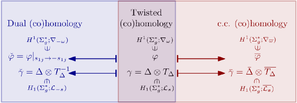
Figure 6: Summary of how the maps $()^{\vee}$ and $\overline{()}$ descend to maps in (co)homology. That is, one only needs to understand how to construct the elements of $H^{1}(\Sigma_{g}^{*};\nabla_{\omega})$ and $H_{1}(\Sigma_{g}^{*};\mathcal{L}_{\boldsymbol{s}})$. The elements of the dual and complex conjugated (co)homologies trivially follow.

5.2 Twisted Riemann bilinear relations and the double copy

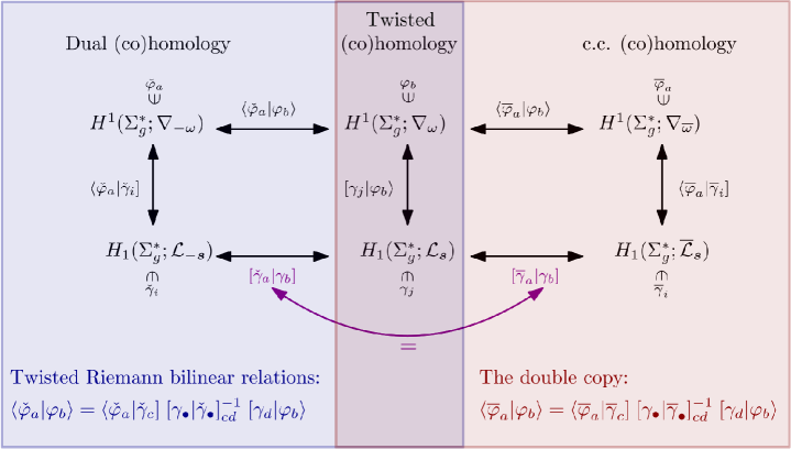
Figure 7: Summary of the introduced twisted (co)homology groups and the various pairings between them: vertical pairings are integration, horizontal pairings are intersection numbers. In particular, the intersection numbers in purple are equal (when $\check{\gamma}$ and $\overline{\gamma}$ are obtained from $\gamma$ as in figure 6).

We have described several twisted (co)homology groups and the various non-degenerate bilinear pairings among them; this is summarized in figure 7. Because these bilinear pairings are compatible with each other, we can use linear algebra to write one in terms of the others. The twisted Riemann bilinear relations (cho1995, , theorem 2) are the twisted version of the usual Riemann bilinear relations (see proposition 5.1); they relate the various pairings between the twisted (co)homologies and their duals (left/blue side of figure 7). On the other hand, the double copy (proposition 5.2) is an analogue of the twisted Riemann bilinear relations where one replaces the dual twisted (co)homologies with the complex conjugated twisted (co)homologies (right/red side of figure 6).

Proposition 5.1.

Twisted Riemann bilinear relations (cho1995, , theorem 2). Let $\check{\varphi}\in H^{1}(\Sigma_{g}^{*},\nabla_{-\omega})$, $\psi\in H^{1}(\Sigma_{g}^{*},\nabla_{\omega})$ be twisted 1-forms and $\langle\varphi|\psi\rangle$ their cohomology intersection number. Let $\{{\gamma}_{a}\}_{a\in\mathcal{K}}$, $\{\check{\gamma}_{b}\}_{b\in\mathcal{J}}$ be bases for their respective twisted homology groups, $\gamma_{a}\in H_{1}(\Sigma_{g}^{*},\mathcal{L}_{\boldsymbol{s}})$, $\check{\gamma}_{b}\in H_{1}(\Sigma_{g}^{*},\mathcal{L}_{-\boldsymbol{s}})$. Denote by $H_{a,b}=[\gamma_{a},\check{\gamma}_{b}]$ the matrix of homology intersection numbers, and $H^{a,b}$ the $(a,b)$-entries of its matrix inverse. Then the twisted Riemann relations hold:

$$\langle\check{\varphi}|\psi\rangle=\sum_{a\in\mathcal{K},b\in\mathcal{J}}H^{a,b}I^{\varphi}_{\gamma_{b}}(z_{1},-s_{1j})I^{\psi}_{\gamma_{a}}(z_{1},s_{1j}).$$ (100)

Proof.

The reader can look at the proof of (cho1995, , theorem 2). More conceptually, we can think of this as a statement in linear algebra: we have 4 finite-dimensional vector spaces with non-degenerate bilinear pairings among them. The matrix element of any one of such pairing can then be written in terms of the others. See (Mizera:2019gea, , Proposition 2.1) for the computation in this linear algebra setting. ∎

As a first example of these relations, consider the cohomology intersection number $\langle\check{\varphi}_{k}|\varphi_{l}\rangle$. Let $\mathcal{K}$ be the following index set of a basis of twisted homology $H_{1}(\Sigma_{g}^{*},\mathcal{L}_{\boldsymbol{s}})$:

$$\mathcal{K}=\{3,4,\ldots,(n-1),A_{1},B_{1},A_{2},B_{2},\ldots,A_{g},B_{g}\}\,,$$ (101)

then, the matrix of homology intersection numbers $\mathbf{H}^{(2,2)}$ introduced in (82) has components given by

$$H^{(2,2)}_{a,b}=[{\gamma}_{2a}|\check{\gamma}_{2b}], a,b\in\mathcal{K}\,.$$ (102)

Then, an example of the Riemann bilinear relations applied on the cohomology intersection number $\langle\check{\varphi}_{k}|\varphi_{l}\rangle$ is:

$$\langle\check{\varphi}_{k}|\varphi_{l}\rangle=\sum_{a,b\in\mathcal{K}}H^{a,b}_{(2,2)}I^{\varphi_{k}}_{\gamma_{b}}(z_{1},-s_{1j})I^{\varphi_{l}}_{\gamma_{a}}(z_{1},s_{1j})\,,$$ (103)

where $H^{a,b}_{(2,2)}$ is the $a,b$- component of the inverse matrix $[\mathbf{H}^{(2,2)}]^{-1}$. We remark that we could have chosen any basis of homology cycles in the formula in (103), and we use this symmetric choice so that the basis of dual integrals is simply related to the basis of non-dual integrals (i.e.  minimize the number of integrals one has to compute).

As a more concrete example, consider the holomorphic differentials $[\omega_{I}]\in H^{1}(\Sigma_{g}^{*},\nabla_{\omega})$, which have a vanishing cohomology intersection numbers with each other (92). Then, the twisted Riemann bilinear relations imply that a certain bilinear combination of hypergeometric integrals $I^{\omega_{J}}_{\gamma_{a}}(z_{i},s_{1j})$ and their duals $I^{\omega_{I}}_{\gamma_{a}}(z_{i},-s_{1j})$ vanishes:

$$\langle\omega_{I}|\omega_{J}\rangle=0=\sum_{a,b\in\mathcal{K}}H^{a,b}_{(2,2)}\bigg[\int_{{\gamma}^{\vee}_{b}}T(z_{1})^{-1}\,\omega_{I}\bigg]\bigg[\int_{{\gamma}_{a}}T(z_{1})\,\omega_{J}\bigg]\,, I,J=1,2,\ldots,g\,.$$ (104)

The twisted Riemann bilinear relations above are the most natural to define, and in the genus-one case have been used to compute differential equations of hypergeometric integrals Mano2012 ; Goto2022 ; bhardwaj2024double . In our work, we found equation (104) useful in performing nontrivial checks of both the homology intersection numbers and numerical implementation of the hypergeometric functions.

We have also introduced the complex hypergeometric integrals $J^{\overline{\varphi_{k}},\varphi_{l}}$, which have an interpretation as cohomology intersection numbers when all the $s_{1\bullet}$ are real, i.e.

$$s_{1\bullet}\in\mathbb{R}, \textrm{for }\bullet\in\{2,3,\ldots,n,A_{1},B_{1},A_{2},B_{2},\ldots,A_{g},B_{g}\}\,.$$ (105)

Thus, there are another four non-degenerate bilinear pairings among twisted homology and cohomology groups. Naturally, one expects an analogue of the twisted Riemann bilinear relations for these.

Proposition 5.2.

Double copy relations (hanamura1999hodge, , equation (5.1)). Let ${\varphi},\psi\in H^{1}(\Sigma_{g}^{*},\nabla_{\omega})$, be twisted 1-forms and $\langle\overline{\varphi},\psi\rangle=J^{\overline{\varphi},\psi}$, and let all the $s_{1\bullet}\in\mathbb{R}$. Let $\{{\gamma}_{a}\}_{a\in\mathcal{K}}$, $\{\check{\gamma}_{b}\}_{b\in\mathcal{J}}$ be bases for their respective twisted homology groups, $\gamma_{a}\in H_{1}(\Sigma_{g}^{*},\mathcal{L}_{\boldsymbol{s}})$, $\check{\gamma}_{b}\in H_{1}(\Sigma_{g}^{*},\mathcal{L}_{-\boldsymbol{s}})$. Denote by $H_{a,b}=[\gamma_{a},\check{\gamma}_{b}]$ the matrix of homology intersection numbers, and $H^{a,b}$ the $(a,b)$-entries of its matrix inverse. Then the double copy relations hold:

$$\langle\overline{\varphi},\psi\rangle=\sum_{a\in\mathcal{K},b\in\mathcal{J}}H^{a,b}\overline{I^{\varphi}_{\gamma_{b}}(z_{1},s_{1j})}I^{\psi}_{\gamma_{a}}(z_{1},s_{1j}).$$ (106)

Proof.

This is just a specialization of the twisted Riemann bilinear relations, and the proof follows similarly. ∎

Using the same homology basis labeled by $\mathcal{K}$, the double copy relations are:

$$J^{\overline{\varphi_{k}},\varphi_{l}}(z_{i},s_{1j})=\sum_{a,b\in\mathcal{K}}H^{a,b}_{(2,2)}\overline{I^{\varphi_{k}}_{\gamma_{b}}(z_{i},s_{1j})}I^{\varphi_{l}}_{\gamma_{a}}(z_{i},s_{1j})\,.$$ (107)

Whenever the integrals $J^{\overline{\varphi_{k}},\varphi_{l}}(z_{i},s_{1j})$, $I^{\varphi_{k}}_{\gamma_{b}}(z_{i},s_{1j})$ and $I^{\varphi_{l}}_{\gamma_{a}}(z_{i},s_{1j})$ converge for all $a,b\in\{3,4,\ldots,n,\linebreak A_{1},B_{1},\ldots,A_{g},B_{g}\}$. There is an elementary proof of this statement in appendix D, with no need for the setup of hanamura1999hodge or twisted (co)homology.

In the physics literature, such bilinear relations are known as KLT relations – following Kawai, Lewellen and Tye Kawai:1985xq – or double copy relations. We will use the latter term to refer to these bilinear relations. A first concrete family of examples of the double copy relations in (107) is obtained, again, from holomorphic differentials $\omega_{I}\in H^{1}(\Sigma_{g}^{*},\nabla_{\omega})$:

$$\int_{\Sigma_{g}^{*}}|T(z_{1})|^{2}\omega_{J}\wedge\overline{\omega_{I}}=\sum_{a,b\in\mathcal{K}}H^{a,b}_{(2,2)}\overline{\bigg[\int_{{\gamma}_{a}}T(z_{1})\,\omega_{I}\bigg]}\bigg[\int_{{\gamma}_{b}}T(z_{1})\,\omega_{J}\bigg]\,.$$ (108)

See the ancillary files for numerical verification of the above relation at genus two.

5.3 Connection to higher-genus string integrals

In this section we make manifest the connection between our “mathematical” twist $T(z_{1})$ and the Koba-Nielsen factor in the chiral splitting formalism of string theory. The Koba-Nielsen $\mathcal{I}_{n}(z_{i},s_{ij},p_{I})$ is an universal factor appearing in the computation of string amplitudes, see e.g. DHoker:1988pdl , and is given by:

$$\begin{aligned} \mathcal{I}_{n}(z_{i},s_{ij},p_{I})&=\exp\bigg\{i\pi\sum_{I,J=1}^{g}\Omega_{IJ}p^{I}\cdot p^{J}+\sum_{I=1}^{g}\sum_{j=1}^{n}2\pi ip^{I}\cdot k_{i}\big(\nu_{I}(z_{i})-\nu_{I}(z_{0})\big)\\ &\phantom{\exp\bigg\{}+\sum_{1\leq i<j\leq n}k_{i}\cdot k_{j}\log E(z_{i},z_{j})\bigg\}\,.\end{aligned}$$ (109)

Here, the $p^{I}\in\mathbb{R}^{10}$ with $I=1,\ldots,g$ are loop momenta, the $k_{i}\in\mathbb{R}^{10}$ with $i=1,\ldots,n$ are the external momenta of the scattered strings, $\cdot$ is the Lorentzian inner product, $z_{j}\in\Sigma_{g}$ are points on a Riemann surface of genus $g$ and $z_{0}\in\Sigma_{g}$ is an arbitrary reference point. Moreover, the $k_{i}$ satisfy the momentum conservation condition:

$$\sum_{j=1}^{n}k_{j}=0\,.$$ (110)

The twist $T(z_{1})$ is highly reminiscent of the chiral splitting Koba-Nielsen factor $\mathcal{I}_{n}$. More specifically, after isolating every term in $\mathcal{I}_{n}$ that contains $z_{1}$, one finds

$$\mathcal{I}_{n}(z_{1})=\exp\bigg\{\sum_{I=1}^{g}\sum_{j=1}^{n}2\pi i\,p^{I}\cdot k_{i}\,\nu_{I}(z_{1})+\sum_{j=2}^{n}s_{1j}\log E(z_{1},z_{j})\bigg\}\,.$$ (111)

This coincides with $T(z_{1})$ after identifying

$$s_{ij} \leftrightarrow k_{i}\cdot k_{j}\,,$$ (112)

$$p^{I}\cdot k_{i} \leftrightarrow s_{1A_{I}}\,.$$ (113)

Next, recall the condition (105) for the reality of the $s_{1\bullet}$. For the $s_{1j}\in\mathbb{R}$, for $j=2,3,\ldots,n$ this is a natural condition since the momenta $k_{i}$ vectors in a real vector space. On the other hand, one often has to complexity the loop momentum $p_{I}$ in order to make sense of string integrals and their analytic continuations. Moreover, the loop momentum is usually unconstrained. Therefore, it is not so obvious how to interpret the reality of $s_{1A_{I}}$ and $s_{1B_{I}}$ in the string theory context.

To find a physical interpretation of the mathematical reality requirements, take the imaginary part of $s_{1B_{J}}$ (c.f., (25)), equate it to zero, and solve for $s_{1A_{I}}$:

$$s_{1A_{I}}=-\sum_{J=1}^{g}Y^{IJ}\sum_{j=2}^{n}s_{1j}\Im[\nu_{J}({z_{j}})]\,,\quad\forall\,I\in\{1,\cdots g\}\,.$$ (114)

Here, $\mathbf{Y}$ is the imaginary part of the $g\times g$ period matrix $Y_{IJ}=\Im(\Omega_{IJ})$. It is a positive definite matrix with an inverse whose components are denoted with raised indices $Y^{IJ}=(Y^{-1})_{IJ}$. In view of (113), the reality condition (114) translates to the following condition on the loop momenta $p^{I}$:

$$p^{I}\rightarrow-\sum_{J=1}^{g}Y^{IJ}\sum_{j=2}^{n}k_{j}\Im[\nu_{J}(z_{j})]\,,$$ (115)

This condition on the loop momentum is exactly the leading substitution rule in string perturbation theory when one performs the loop momentum integration after massaging the integrand into a Gaussian form. In other words, (115) corresponds to the saddle point of a Gaussian integral. See first line of (Mafra:2018pll, , equation (7.13)) for a genus-one example.

To see how the reality of $s_{1A_{I}}$ and $s_{1B_{I}}$ effect the double copy, substitute (114) into the factor of $|T(z_{1})|^{2}$ in the integrand of the complex hypergeometric integral $J^{\overline{\varphi_{k}}\varphi_{l}}$. Before substituting, we do a small rewriting of $|T(z_{1})|^{2}$:

$$|T(z_{1})|^{2} =\exp\bigg\{-4\pi\sum_{J=1}^{g}s_{1A_{J}}\Im[\nu_{J}(z_{1})]+\sum_{j=2}^{n}s_{1j}\log|E(z_{1},z_{j})|^{2}\bigg\}\,.$$ (116)

Next, we substitute (114) into $|T(z_{1})|^{2}$:

$$|T(z_{1})|^{2}\bigg|_{\eqref{eq:reality_condition_solving}} =\exp\bigg\{4\pi\sum_{I,J=1}^{g}\sum_{j=2}^{n}s_{1j}Y^{IJ}\Im[\nu_{I}(z_{j})]\Im[\nu_{J}(z_{1})]+\sum_{j=2}^{n}s_{1j}\log|E(z_{1},z_{j})|^{2}\bigg\}$$

$$=\exp\left\{\sum_{j=2}^{n}s_{1j}\bigg[\log|E(z_{1},z_{j})|^{2}+4\pi\sum_{I,J=1}^{g}Y^{IJ}\Im[\nu_{I}(z_{j})]\Im[\nu_{J}(z_{1})]\bigg]\right\}$$

$$=\exp\left\{\sum_{j=2}^{n}s_{1j}\bigg[G(z_{1},z_{j})+2\pi\sum_{I,J=1}^{g}Y^{IJ}\Im[\nu_{I}(z_{j})]\Im[\nu_{J}(z_{j})]\bigg]\right\}\,,$$ (117)

where we have introduced the string Green’s function $G(z_{1},z_{j})$, which is single-valued for $z_{1},z_{j}\in\Sigma_{g}$:

$$G(z_{1},z_{j})=\log|E(z_{1},z_{j})|^{2}-2\pi\sum_{I,J=1}^{g}Y^{IJ}\Im[\nu_{I}(z_{1})-\nu_{I}(z_{j})]\Im[\nu_{J}(z_{1})-\nu_{J}(z_{j})]\,.$$ (118)

Note that we have “completed the square” in the computation of (118), and we further used momentum conservation to show that the $j$-independent term vanishes:

$$\sum_{j=2}^{n}s_{1j}\sum_{I,J=1}^{g}2\pi\sum_{I,J=1}^{g}Y^{IJ}\Im[\nu_{I}(z_{1})]\Im[\nu_{J}(z_{1})]=0\,.$$ (119)

In view of this computation, we can write the double-copy relations in (107) in terms of the string Green’s function, after multiplying both sides by some $z_{1}$-independent factors:

$$\int_{z_{1}\in\Sigma_{g}^{*}}\varphi_{l}\wedge\overline{\varphi}_{k}\exp\bigg[\sum_{j=2}^{n}s_{1j}G(z_{1},z_{j})\bigg]= \exp\bigg[-2\pi\sum_{j=2}^{n}s_{1j}\ \sum_{I,J=1}^{g}Y^{IJ}\Im[\nu_{I}(z_{j})]\Im[\nu_{J}(z_{j})]\bigg]$$

$$\phantom{=}\times\sum_{a,b\in\mathcal{K}}H^{a,b}_{(2,2)}\overline{\bigg[\int_{{\gamma}_{b}}T(z_{1})\,\varphi_{k}\bigg]}\bigg[\int_{{\gamma}_{a}}T(z_{1})\,\varphi_{l}\bigg]\bigg|_{\eqref{eq:reality_condition_solving}}\,.$$ (120)

Thus, we have obtained a double-copy formula at genus $g$, closely related to string amplitudes, coming from twisted (co)homology.

6 Abelian Kronecker forms and higher genus polylogarithms

In the previous section, we derived double-copy formulas involving single-valued $1$-forms $\varphi$. So far, the $\varphi$ are either holomorphic differentials or meromorphic differentials with poles of order one or two (c.f., (3.1)). However, for string theory practitioners, these are not expected to be enough. To address this, various groups in the physics and mathematics literature Enriquez:2011np ; enriquez2021construction ; DHoker:2023vax ; Baune:2024biq have introduced a richer family of $1$-forms, called Enriquez kernels, ${g^{I_{1},I_{2},\ldots,I_{r}}}_{J}(z_{1},z_{j})$, for $r\in\mathbb{Z}_{\geq 0}$, with the convention that ${g^{\varnothing}}_{J}(z_{1},z_{j})=\omega_{J}(z_{1})\text{d}z_{1}$ is a normalized holomorphic differential. The $1$-forms, ${g^{I_{1},I_{2},\ldots,I_{r}}}_{J}(z_{1},z_{j})$ are meromorphic but not single-valued $1$-forms on $z_{1}\in\Sigma_{g}$, and $0$-forms in $z_{j}\in\Sigma_{g}$. They provide integration kernels for polylogarithms on Riemann surfaces of genus $g\geq 1$. For a friendly introduction to these kernels, see DHoker:2023vax ; Baune:2024biq ; DHoker:2025dhv . Using the integration kernels ${g^{I_{1},I_{2},\ldots,I_{r}}}_{J}(z_{1},z_{j})$, we introduce an alternative version of the genus-$g$ hypergeometric integrals in this section.

The $1$-forms ${g^{I_{1},I_{2},\ldots,I_{r}}}_{J}(z_{1},z_{j})$ can be obtained from $J=1,\ldots,g$ form-valued generating functions, $F_{J}(z_{1},z_{j},\alpha_{I})$:

$$F_{J}(z_{1},z_{j},\alpha_{I})\,\alpha_{J}=\sum_{r\geq 0}\sum_{I_{1},I_{2},\ldots,I_{r}=1}^{g}{g^{I_{1},I_{2},\ldots,I_{r}}}_{J}(z_{1},z_{j})\alpha_{I_{1}}\alpha_{I_{2}}\ldots\alpha_{I_{r}}\,,$$ (121)

where the $\alpha_{j}$, $j=1,\ldots,g$ are formal, non-commutative variables (Baune:2024biq, , (5.23)). These $1$-forms $F_{J}(z_{1},z_{j})$ have prescribed monodromies

$$F_{J}(z_{1}+\mathfrak{A}_{I},z_{j},\alpha_{I}) =F_{J}(z_{1},z_{j},\alpha_{I})\,, F_{J}(z_{1}+\mathfrak{B}_{I},z_{j},\alpha_{I}) =\exp(-2\pi i\alpha_{I})F_{J}(z_{1},z_{j},\alpha_{I})\,,$$ (122)

and $\mathfrak{A}$-cycle periods

$$\oint_{\mathfrak{A}_{I}}F_{J}(z_{1},z_{j},\alpha_{I}) =\frac{\delta_{IJ}}{\exp(2\pi i\alpha_{J})-1}\,, \operatornamewithlimits{res}_{(z_{1},z_{j})}F_{J}(z_{1},z_{j},\alpha_{j}) =1\,,$$ (123)

where $I,J=1\ldots,g$ Lisitsyn_masters_thesis . The $1$-forms $F_{J}(z_{1},z_{j},\alpha_{I})$ were first introduced in Baune:2024biq , denoted by $S_{j}(z_{1},z_{j},\alpha_{I})$ and called Schottky-Kronecker forms. In this work, we refer to the $1$-forms $F_{J}(z_{1},z_{j},\alpha_{I})$ as Kronecker forms. Closely related connections on punctured Riemann surfaces have also appeared in other recent works in both physics and mathematics bernard1988wess ; DHoker:2023vax .

From this point onward, we specialize to Abelian Kronecker forms: genus-$g$ generalizations of the genus-one Kronecker-Eisenstein series Broedel:2014vla . The Abelian Kronecker forms are obtained from the non-Abelian versions by interpreting the $\alpha_{J}$ as commuting variables or setting $\alpha_{J}\in\mathbb{C}$. These forms define another family of genus $g$ hypergeometric integrals with a direct, albeit somewhat limited, connection to higher genus polylogarithms. For example, we cannot extract ${g(z_{1},z_{j})^{1,2}}_{2}$ from the Abelian Kronecker form by isolating the $\alpha_{1}\alpha_{2}$-coefficient of $F_{2}(z_{1},z_{j},\alpha_{I})\,\alpha_{2}$. Instead, one obtains the linear combination

$$\alpha_{1}\alpha_{2}\textrm{- coefficient of }F_{2}(z_{1},z_{j},\alpha_{I})\alpha_{2}:{g(z_{1},z_{j})^{1,2}}_{2}+{g(z_{1},z_{j})^{2,1}}_{2}\,.$$ (124)

On the other hand, we can isolate the term ${g(z_{1},z_{j})^{I}}_{J}$, $I=1,\ldots,g$ unambiguously from Abelian Kronecker forms $F_{J}(z_{1},z_{j},\alpha_{I})\,\alpha_{J}$.

6.1 Twisted (co)homology with Abelian Kronecker forms

To widen the applicability of the techniques and results presented so far, we generalize the genus-$g$ hypergeometric functions and their associated twisted (co)homology to allow for Abelian Kronecker forms in the integrand. This creates a direct link to certain higher genus polylogarithms.

Let $\alpha_{J},J=1,2,\ldots,g$ be complex-valued parameters and let $\varphi^{\boldsymbol{\alpha}}$ be quasiperiodic forms on $\Sigma_{g}^{*}$ that satisfy

$$\varphi^{\boldsymbol{\alpha}}(z_{1}+\mathfrak{A}_{J}) =\varphi^{\boldsymbol{\alpha}}(z_{1})\,, J=1,2,\ldots,g\,,$$

$$\varphi^{\boldsymbol{\alpha}}(z_{1}+\mathfrak{B}_{J}) =\exp(-2\pi i\alpha_{J})\varphi^{\boldsymbol{\alpha}}(z_{1})\,, J=1,2,\ldots,g\,.$$ (125)

That is, the $\varphi^{\boldsymbol{\alpha}}$ have the same quasiperiodicity as Abelian Kronecker forms, $F_{j}(z_{1},z_{j},\alpha_{I})$ (c.f., (122)). In this section, we consider the twisted cohomology associated to the integrals

$$I^{\varphi}_{\gamma}(z_{i},s_{ij},\alpha_{I})=\int_{\gamma^{\boldsymbol{\alpha}}}T(z_{1})\varphi^{\boldsymbol{\alpha}}(z_{1})\,.$$ (126)

Once we have characterized this (co)homology, the double copy construction of section 5 straightforwardly generalizes.

Let $\mathcal{L}_{\boldsymbol{\alpha}}$ be the local system encoding the multivaluedness of the $1$-forms $\varphi^{\boldsymbol{\alpha}}$ and $\mathcal{L}_{\boldsymbol{s}}\otimes\mathcal{L}_{\boldsymbol{\alpha}}$ the local system encoding the multivaluedness of the integrand $T(z_{1})\varphi^{\boldsymbol{\alpha}}$. Then, we can think of the integral (126) as a pairing between the associated twisted homology and twisted cohomology

$$\gamma^{\boldsymbol{\alpha}}\in H_{1}(\Sigma_{g}^{*},\mathcal{L}_{\boldsymbol{s}}\otimes\mathcal{L}_{\alpha_{I}})\,,\qquad\varphi^{\boldsymbol{\alpha}}\in H^{1}(\Sigma^{*}_{g},\mathcal{L}_{\boldsymbol{\alpha}},\nabla_{\omega})\,.$$ (127)

The structure of twisted homology is essentially the same as before, just with a new local system that keeps track of the multivaluedness of twist and quasiperiodicity of the differential form ($T\varphi^{\boldsymbol{\alpha}}$): $\mathcal{L}_{\boldsymbol{s}}\otimes\mathcal{L}_{\boldsymbol{\alpha}}$. For the most part, the structure of the twisted cohomology is unchanged. We still use the twisted differential $\nabla_{\omega}$. It just acts on 1-forms $\varphi^{\boldsymbol{\alpha}}$ valued in $\mathcal{L}_{\boldsymbol{\alpha}}$ (quasiperiodic along the $B$-cycles): $\varphi^{\boldsymbol{\alpha}}\in\Omega^{1}(\Sigma_{g}^{*},\mathcal{L}_{\boldsymbol{\alpha}})$. Explicitly,

$$H^{k}(\Sigma_{g}^{*},\mathcal{L}_{\alpha_{I}},\nabla_{\omega})=\frac{\operatorname{Ker\left(\nabla_{\omega}:\Omega^{k}(\Sigma_{g}^{*},\mathcal{L}_{\boldsymbol{\alpha}})\rightarrow\Omega^{k+1}(\Sigma_{g}^{*},\mathcal{L}_{\boldsymbol{\alpha}})\right)}}{\operatorname{Im\left(\nabla_{\omega}:\Omega^{k-1}(\Sigma_{g}^{*},\mathcal{L}_{\boldsymbol{\alpha}})\rightarrow\Omega^{k}(\Sigma_{g}^{*},\mathcal{L}_{\boldsymbol{\alpha}})\right)}}\,,$$ (128)

where $\Omega^{k}(\Sigma_{g}^{*},\mathcal{L}_{\boldsymbol{\alpha}})$ denotes the $\alpha_{I}$-quasiperiodic $k$-forms on the punctured Riemann surface $\Sigma_{g}^{*}$. Following Watanabe, we can describe this twisted cohomology group.

Proposition 6.1.

Under the condition $n>\max(2,2g-1)$, the first twisted cohomology group of a punctured Riemann surface of genus $g$, $H^{1}(\Sigma_{g}^{*},\mathcal{L}_{\boldsymbol{\alpha}},\nabla_{\omega})$, is spanned by ${\boldsymbol{\alpha}}$-quasiperiodic 1-forms:

$$H^{1}(\Sigma_{g}^{*},\mathcal{L}_{\boldsymbol{\alpha}},\nabla_{\omega})={\operatorname{span}}( {\omega}^{\boldsymbol{\alpha}}_{1},{\omega}^{{\boldsymbol{\alpha}}}_{2},\ldots,{\omega}^{{\boldsymbol{\alpha}}}_{g-1},{\tau}^{{\boldsymbol{\alpha}}}_{z_{2}}(z_{1}),{\tau}^{{\boldsymbol{\alpha}}}_{z_{3}}(z_{1}),\ldots,{\tau}^{{\boldsymbol{\alpha}}}_{z_{g}}(z_{1}),$$

$${\sigma}^{{\boldsymbol{\alpha}}}_{z_{2}}(z_{1}),{\sigma}^{\boldsymbol{\alpha}}_{z_{3}}(z_{1}),\ldots,{\sigma}^{\boldsymbol{\alpha}}_{z_{n}}(z_{1}))\,.$$ (129)

Here, the ${\omega}^{\boldsymbol{\alpha}}_{j}$ are holomorphic ${\boldsymbol{\alpha}}$-quasiperiodic differentials, ${\tau}^{\boldsymbol{\alpha}}_{z_{j}}(z_{1})$ are meromorphic ${\boldsymbol{\alpha}}$-quasiperiodic differentials with a unique pole of order 2 at $z_{j}$, and ${\sigma}^{\boldsymbol{\alpha}}_{z_{j}}(z_{1})$ are meromorphic $\boldsymbol{\alpha}$-quasiperiodic differentials with a unique pole of order 1 at $z_{j}$, with unit residue. In particular, we can take ${\sigma}^{\boldsymbol{\alpha}}_{z_{j}}(z_{1})=F(z_{1},z_{j},\alpha_{I})$. That is, for $n>\max(2,2g-1)$, we have $\operatorname{dim}H^{1}(\Sigma_{g}^{*},\mathcal{L}_{\boldsymbol{\alpha}},\nabla_{\omega})=(2g+n-3)$, and this twisted cohomology can be spanned by ${\boldsymbol{\alpha}}$-quasiperiodic differentials that include the Abelian Kronecker forms.

Proof.

This is essentially the content of (watanabe2016twisted, , theorem 4.1 and example 1). Watanabe proves a theorem with $k$-forms valued in a line bundle $P$, and if we use $P=\mathcal{L}_{\boldsymbol{\alpha}}$ the proof goes through exactly the same way. Because $\mathcal{L}_{\boldsymbol{\alpha}}$ has trivial Chern class, the twisted cohomology is described explicitly as in (watanabe2016twisted, , example 1). ∎

As an interesting remark, we note that the space of holomorphic $\alpha_{I}$-quasiperiodic 1-forms on a compact Riemann surface of genus $g$ has dimension $g-1$. This explains why only $(g-1)$ such forms appear in the basis of $H^{1}(\Sigma_{g}^{*},\mathcal{L}_{\alpha_{I}},\nabla_{\omega})$. A nice proof of this fact can be found in section 6.3 of Lisitsyn_masters_thesis .

The locally finite twisted homology $H_{1}^{l\!f}(\Sigma_{g}^{*},\mathcal{L}_{\boldsymbol{s}}\otimes\mathcal{L}_{\boldsymbol{\alpha}})$ is easy to obtain from $H_{1}^{l\!f}(\Sigma_{g}^{*},\mathcal{L}_{\boldsymbol{s}})$. It is spanned by the same set of twisted cycles (c.f., (55)) where one replaces the loading from $\mathcal{L}_{\boldsymbol{s}}$ with one from $\mathcal{L}_{\boldsymbol{s}}\otimes\mathcal{L}_{\boldsymbol{\alpha}}$. Similarly, the regularized twisted cycles of $H_{1}(\Sigma_{g}^{*},\mathcal{L}_{\boldsymbol{s}}\otimes\mathcal{L}_{\boldsymbol{\alpha}})$ are simply related to those of $H_{1}(\Sigma_{g}^{*},\mathcal{L}_{\boldsymbol{s}})$. To see this, recall that the local systems $\mathcal{L}_{\boldsymbol{s}}\otimes\mathcal{L}_{\boldsymbol{\alpha}}$ and $\mathcal{L}_{\boldsymbol{s}}$ are $\pi_{1}$-bundles where we use the 1-dimensional representation for the monodromies $\rho:\pi_{1}(\Sigma_{g}^{*},*)\to\mathbb{C}^{*}$ (c.f., (33)). Thus, the representation for the local system $\mathcal{L}_{\boldsymbol{s}}\otimes\mathcal{L}_{\boldsymbol{\alpha}}$ is given by the product of representations for $\mathcal{L}_{\boldsymbol{s}}$ and $\mathcal{L}_{\boldsymbol{\alpha}}$: $\rho^{\boldsymbol{s},\boldsymbol{\alpha}}=\rho\times\rho^{\boldsymbol{\alpha}}$. Explicitly,

$$\rho^{\boldsymbol{s},\boldsymbol{\alpha}}(M_{i}) :=e^{2\pi is_{1i}}\,, \rho^{\boldsymbol{s},\boldsymbol{\alpha}}(\mathfrak{A}_{I}) :=e^{2\pi is_{1A_{I}}}\,, \rho^{\boldsymbol{s},\boldsymbol{\alpha}}(\mathfrak{B}_{I}) :=e^{2\pi i(s_{1B_{I}}-\alpha_{I})}\,,$$ (130)

where $i=2,\dots,n$, $I=1,\dots,g$, and $\rho^{\boldsymbol{\alpha}}(\mathfrak{B}_{I})=e^{-2\pi\alpha_{I}}$ is the only non-trivial monodromy associated to $\mathcal{L}_{\boldsymbol{\alpha}}$. The twisted homology $H_{1}(\Sigma_{g}^{*},\mathcal{L}_{\boldsymbol{s}}\otimes\mathcal{L}_{\boldsymbol{\alpha}})$ is spanned by the cycles in (4.2) after making the substitution

$$s_{1B_{J}}\rightarrow s_{1B_{J}}-\alpha_{J}\,, J=1,\ldots,g\,.$$ (131)

We note that this is also the case in the genus-one case, as seen in Mano2012 .

There is also the dual twisted (co)homology groups:

$$\big(H_{1}(\Sigma_{g}^{*},\mathcal{L}_{\boldsymbol{s}}\otimes\mathcal{L}_{\boldsymbol{\alpha}})\big)^{\vee}:=H_{1}(\Sigma_{g}^{*},\mathcal{L}_{-\boldsymbol{s}}\otimes\mathcal{L}_{-\boldsymbol{\alpha}})\,,\qquad\big(H^{1}(\Sigma_{g}^{*},\mathcal{L}_{\boldsymbol{\alpha}},\nabla_{\omega})\big)^{\vee}:=H_{1}(\Sigma_{g}^{*},\mathcal{L}_{-\boldsymbol{\alpha}},\nabla_{-\omega})$$ (132)

where the dualizing operator $()^{\vee}$ also changes the sign of the all the $\alpha_{I}$: $(\bullet)^{\vee}=\bullet|_{s_{1j}\to-s_{1j},\alpha_{I}\to-\alpha_{I}}$. Using the dual (co)homology one can define the usual intersection pairings (62) and (LABEL:eq:coho_int_num). Fortunately, the intersection numbers of the $\boldsymbol{\alpha}$-quasiperiodic twisted (co)homology are obtained by simply applying the substitution (131):

$$\langle\check{\varphi}^{\boldsymbol{\alpha}}_{k}|\varphi^{\boldsymbol{\alpha}}_{l}\rangle =\langle\check{\varphi}_{k}|\varphi_{l}\rangle|_{s_{1B_{J}}\to s_{1B_{J}}-\alpha_{J}}\,, [\gamma^{\boldsymbol{\alpha}}_{k}|\check{\gamma}^{\boldsymbol{\alpha}}_{l}] =[\gamma_{k}|\check{\gamma}_{l}]|_{s_{1B_{J}}\to s_{1B_{J}}-\alpha_{J}}\,.$$ (133)

6.2 Homology intersection numbers and complex hypergeometric integrals

We also introduce complex hypergeometric integrals with $\boldsymbol{\alpha}$-quasiperiodic forms, of the form:

$$J^{\overline{\varphi_{k}},\varphi_{l}}(z_{j},s_{ij},\alpha_{I})=\int_{\Sigma_{g}^{*}}|T(z_{1})|^{2}\,\varphi^{\boldsymbol{\alpha}}_{l}\wedge\overline{\varphi^{\boldsymbol{\alpha}}_{k}}\,.$$ (134)

In the remainder of this section, we describe how to understand (134) as a cohomology intersection number. Then, in the next section, we derive a double copy for these integrals.

To do this, we need to introduce the complex conjugated local system $\overline{\mathcal{L}_{\boldsymbol{s}}\otimes{\mathcal{L}_{\boldsymbol{\alpha}}}}$, which takes into account the multivaluedness of $\overline{T(z_{1})\varphi^{\boldsymbol{\alpha}}}$. This local system is naturally isomorphic to $\mathcal{L}_{-\boldsymbol{s}}\otimes{\mathcal{L}_{-\boldsymbol{\alpha}}}$ whenever:

$$(s_{1B_{J}}-\alpha_{J})\in\mathbb{R}\,, J=1,2,\ldots,g\,.$$ (135)

Thus, assuming (135) the integral (134) forms a non-degenerate pairing between the twisted cohomology groups $H^{1}({\Sigma_{g}^{*}},\mathcal{L}_{\boldsymbol{\alpha}},\nabla_{\omega})$ and $H^{1}(\Sigma_{g}^{*},\overline{\mathcal{L}_{\boldsymbol{\alpha}}},\nabla_{\overline{\omega}})$ whenever it converges (analogous to (LABEL:eq:coho_int_num)). Thus, we interpret the complex hypergeometric integral of $\alpha_{I}$-quasiperiodic $1$-forms as a pairing of twisted cohomology groups:

$$\langle\overline{\bullet}|\bullet\rangle:H^{1}(\Sigma_{g}^{*},\overline{\mathcal{L}_{\boldsymbol{s}}\otimes\mathcal{L}_{\alpha}})\times H^{1}({\Sigma_{g}^{*}},{\mathcal{L}_{\boldsymbol{s}}\otimes\mathcal{L}_{\alpha}})\rightarrow\mathbb{C}\,\quad\text{via}\quad(\overline{\varphi^{\boldsymbol{\alpha}}_{k}},\varphi^{\boldsymbol{\alpha}}_{l})\mapsto\langle\overline{\varphi^{\boldsymbol{\alpha}}_{k}}|\varphi^{\boldsymbol{\alpha}}\rangle\,,$$ (136)

where

$$J^{\overline{\varphi_{k}},\varphi_{l}}(z_{j},s_{ij},\alpha_{I})=\langle\overline{\varphi^{\boldsymbol{\alpha}}_{k}}|\varphi^{\boldsymbol{\alpha}}_{l}\rangle:=\int_{\Sigma_{g}^{*}}|T(z_{1})|^{2}\,\varphi^{\boldsymbol{\alpha}}_{l}\wedge\overline{\varphi^{\boldsymbol{\alpha}}_{k}}=J^{\overline{\varphi_{k}},\varphi_{l}}\,.$$ (137)

Of course, there is also the complex conjugated twisted homology $H_{1}(\Sigma_{g}^{*},\overline{\mathcal{L}_{\boldsymbol{s}}\otimes\mathcal{L}_{\boldsymbol{\alpha}}})$ which can be paired with $H^{1}(\Sigma_{g}^{*},\overline{\mathcal{L}_{\boldsymbol{\alpha}}},\nabla_{\overline{\omega}})$ in the usual way

$$\overline{I^{\varphi}_{\gamma}}: H_{1}(\Sigma_{g}^{*},\overline{\mathcal{\check{L}\otimes}\mathcal{L}_{\alpha_{I}}})\times H^{1}(\Sigma_{g}^{*},\overline{\mathcal{L}_{\boldsymbol{s}}\otimes\mathcal{L}_{\alpha}})\rightarrow\mathbb{C}\,,$$

via

$$(\gamma,\overline{\varphi}) \mapsto\langle\overline{\varphi^{\boldsymbol{\alpha}}}|\overline{\gamma}]:=\int_{\overline{\gamma}}\overline{\varphi^{\boldsymbol{\alpha}}}=\overline{\int_{\gamma}T(z_{1})\varphi^{\boldsymbol{\alpha}}}=\overline{[\gamma^{\boldsymbol{\alpha}}|\varphi^{\boldsymbol{\alpha}}\rangle}\,,$$ (138)

whenever the condition (135) is satisfied. In particular, recall that the homology intersection numbers of complex conjugated cycles are equal to those of the dualized cycles

$$[\gamma_{l}|\overline{\gamma}_{k}] =[\gamma_{l}|\check{\gamma}_{k}]\,.$$ (139)

Therefore, we can avoid performing any new calculations to construct the double copy of Abelian Kronecker forms.

6.3 The double copy of Abelian Kronecker forms

In this section we flesh out the double copy for the complex hypergeometric integral of $\boldsymbol{\alpha}$-quasiperiodic 1-forms in (134). These relations are, once again, obtained from the compatibility of the non-degenerate pairings among homology and cohomology groups (see figure 7). Explicitly,

$$\int_{\Sigma_{g}^{*}}|T(z_{1})|^{2}\,\varphi^{\boldsymbol{\alpha}}_{l}\wedge\overline{\varphi^{\boldsymbol{\alpha}}_{k}}=\sum_{a,b\in\mathcal{K}}\tilde{H}^{a,b}_{(2,2)}\overline{\bigg[\int_{{\gamma}_{b}}T(z_{1})\,\varphi^{\boldsymbol{\alpha}}_{k}\bigg]}\bigg[\int_{{\gamma}_{a}}T(z_{1})\,\varphi^{\boldsymbol{\alpha}}_{l}\bigg]\,,$$ (140)

where, the entries $\tilde{H}^{a,b}_{(2,2)}$ are obtained from the ones that enter in (103) after applying the substitution in (131), and requiring that $(s_{1B_{J}}-\alpha_{J})\in\mathbb{R}$ for $J=1,\ldots,g$ .

For a concrete example, consider the case of Abelian Kronecker forms:

$$\int_{\Sigma_{g}^{*}}|T(z_{1})|^{2} \,{F_{K}(z_{1},z_{3},\alpha_{I})}\wedge\overline{F_{J}(z_{1},z_{2},\alpha_{I})}$$

$$=\sum_{a,b\in\mathcal{K}}\tilde{H}^{a,b}_{(2,2)}\overline{\bigg[\int_{{\gamma}_{b}}T(z_{1})\,F_{J}(z_{1},z_{2},\alpha_{I})\bigg]}\bigg[\int_{{\gamma}_{a}}T(z_{1})\,F_{K}(z_{1},z_{3},\alpha_{I})\bigg]\,.$$ (141)

We can ensure the reality of $s_{1B_{J}}-\alpha_{J}$ by setting

$$s_{1A_{I}}=\sum_{J=1}^{g}Y^{IJ}\Im(\alpha_{J})-\sum_{J=1}^{g}Y^{IJ}\sum_{j=2}^{n}s_{1j}\Im\big[\nu_{J}(z_{j})\big]\,\,\,I=1,\ldots,g\,.$$ (142)

This condition is analogous to (114). After specializing $s_{1A_{I}}$, $|T(z_{1})|^{2}$ is given by (117) with an extra $\alpha_{I}$-dependent factor:

$$|T(z_{1})|^{2}\bigg|_{\eqref{eq:reality_condition_solving_alpha}} =(\textrm{RHS of \eqref{eq:Tofz1Sq_after_substitution}})\times\exp\bigg[-4\pi\sum_{I,J=1}^{g}Y^{IJ}\Im[\alpha_{J}]\Im[\nu_{I}(z_{1})]\bigg]\,,$$

$$=(\textrm{RHS of \eqref{eq:Tofz1Sq_after_substitution}})\times\exp\bigg[2\pi i\sum_{I,J=1}^{g}Y^{IJ}\Im[\nu_{I}(z_{1})](\alpha_{J}-\overline{\alpha_{J}})\bigg]\,.$$ (143)

Then, note that the combination

$$\Omega_{J}(z_{1},z_{j},\alpha_{I})=\exp\bigg[2\pi i\sum_{M,N=1}^{g}Y^{MN}\Im[\nu_{M}(z_{1})]\alpha_{N}\bigg]F_{J}(z_{1},z_{j},\alpha_{I})\,,$$ (144)

is a single-valued (in $z_{1}$) version of the Abelian Kronecker form. Often in the string theory literature, it is advantageous to trade meromorphic forms (e.g., $F_{J}(z_{1},z_{j},\alpha_{I})$) for non-meromorphic but single-valued forms (e.g., $\Omega_{J}(z_{1},z_{j},\alpha_{I})$).

Using $\Omega_{J}(z_{1},z_{j},\alpha_{I})$ in the double copy formula (6.3), after using the substitution (142), yields

$$\int_{\Sigma_{g}^{*}} {\Omega_{K}(z_{1},z_{3},\alpha_{I})}\wedge\overline{\Omega_{J}(z_{1},z_{2},\alpha_{I})_{J}}\exp\bigg[\sum_{j=2}^{n}s_{1j}G(z_{1},z_{j})\bigg]$$

$$=\exp\bigg[-2\pi\sum_{j=2}^{n}s_{1j}\ \sum_{I,J=1}^{g}Y^{IJ}\Im[\nu_{I}(z_{j})]\Im[\nu_{J}(z_{j})]\bigg]$$

$$\phantom{=}\times\sum_{a,b\in\mathcal{K}}\tilde{H}^{a,b}_{(2,2)}\overline{\bigg[\int_{{\gamma}_{b}}T(z_{1})\,F_{J}(z_{1},z_{2},\alpha_{I})\bigg]}\bigg[\int_{{\gamma}_{a}}T(z_{1})\,F_{K}(z_{1},z_{3},\alpha_{I})\bigg]\bigg|_{\eqref{eq:reality_condition_solving_alpha}}\,.$$ (145)

This is an explicit double copy formula for integrals of single-valued Abelian Kronecker forms, $\Omega_{J}(z_{1},z_{j},\alpha_{I})$, and the string Green’s functions, $G(z_{1},z_{j})$.

7 examples in genus 2

In this section we present two explicit examples of the double-copy relations of hypergeometric integrals at genus two. For simplicity, we set $n=3$ in both examples . That is, $\Sigma_{2}^{*}$ is a genus-two Riemann surface two punctures, $z_{2},z_{3}$. With $(n,g)=(3,2)$, the relevant twisted (co)homology groups are $(2(2)+3-3=4)$-dimensional (c.f., (3.1) and (6.1)). In the first example, we present the double copy of holomorphic differentials in the context of section 5. We also spell out the matrix $[\mathbf{H}^{(22)}]^{-1}$. After making the substitution (131), this matrix becomes the (the analogue of the) KLT kernel for our second example involving the $\boldsymbol{\alpha}$-quasiperiodic integrands. Moreover, we make a connection to an integration kernel of higher-genus polylogarithms.

7.1 A genus-two double copy formula with holomorphic differentials

Consider a genus two Riemann surface with two punctures $z_{2},z_{3}$: $\Sigma_{g}^{*}$. With $(n,g)=(3,2)$, the relevant twisted (co)homology groups are 4-dimensional. The twisted homology is spanned by five-cycles

$$H_{1}(\Sigma_{g}^{*},\mathcal{L}_{\boldsymbol{s}})=\mathrm{span}\{\gamma_{2A_{I}},\gamma_{2B_{I}},\gamma_{23}\}\,,\qquad I=1,2\,,$$ (146)

subject to the relation

$$0 =\sum_{I=1}^{2}\left(1-e^{2\pi is_{1B_{I}}}\right)[{\gamma}_{2A_{I}}]+\sum_{I=1}^{2}\left(e^{2\pi is_{1A_{I}}}-1\right)[{\gamma}_{2B_{I}}]+\left(e^{-2\pi is_{12}}-1\right)[{\gamma}_{23}]\,\,,$$ (147)

(c.f., equations (4.2), (4.1), (55) and (4.3)). In this and the next example, we choose a basis consisting of only the $A_{I}$- and $B_{I}$-cycles. A basis for cohomology is not needed, since we restrict the example to exemplifying the double copy of holomorphic forms $J^{(g=2)}(z_{j},s_{ij})=\langle\overline{\omega}_{1}|\omega_{2}\rangle$.

Explicitly, $J^{(g=2)}(z_{j},s_{ij})$ is

$$J^{(g=2)}(z_{j},s_{ij}) =\phantom{=}\int_{\Sigma_{2}^{*}}\omega_{2}\wedge\overline{\omega_{1}}\,|T(z_{1})|^{2}\,$$

$$=\int_{\Sigma_{2}^{*}}\omega_{2}\wedge\overline{\omega_{1}}\,\bigg|\exp\bigg(2\pi i\big[s_{1A_{1}}\nu_{1}(z_{1})+s_{1A_{2}}\nu(z_{1})\big]\bigg)\bigg|^{2}\bigg|\frac{E(z_{1},z_{2})}{E(z_{1},z_{3})}\bigg|^{2s_{12}}\,,$$ (148)

where we use momentum conservation $s_{13}=-s_{12}$ and fix our branch cuts so that

$$T(z_{1})=e^{2\pi i[s_{1A_{1}}\nu_{2}(z_{1})+s_{1A_{1}}\nu_{2}(z_{1})]}\bigg[\frac{E(z_{1},z_{2})}{E(z_{1},z_{3})}\bigg]^{s_{12}}\,.$$ (149)

Furthermore, $J^{(g=2)}(z_{j},s_{ij})$ converges for $-1<s_{12}<1$. To use equation (108), on the genus-two integral $J^{(g=2)}(z_{j},s_{ij})$, we need the inverse of the intersection matrix $\mathbf{H}^{(2,2)}$ as well as the vectors of integrals

$$\mathbf{I}_{1}^{(g=2)}=\begin{pmatrix}\int_{\gamma_{2A_{1}}}T(z_{1})\,\omega_{1}\\ \int_{\gamma_{2B_{1}}}T(z_{1})\,\omega_{1}\\ \int_{\gamma_{2A_{2}}}T(z_{1})\,\omega_{1}\\ \int_{\gamma_{2B_{2}}}T(z_{1})\,\omega_{1}\end{pmatrix}\,, \mathbf{I}_{2}^{(g=2)}=\begin{pmatrix}\int_{\gamma_{2A_{1}}}T(z_{1})\,\omega_{2}\\ \int_{\gamma_{2B_{1}}}T(z_{1})\,\omega_{2}\\ \int_{\gamma_{2A_{2}}}T(z_{1})\,\omega_{2}\\ \int_{\gamma_{2B_{2}}}T(z_{1})\,\omega_{2}\end{pmatrix}\,.$$ (150)

Here, each integral in $\mathbf{I}_{1}^{(g=2)}$ and $\mathbf{I}_{2}^{(g=2)}$ converge for $s_{12}>-1$. These integrals are computed numerically, while the inverse intersection matrix is know analytically.

To present the inverse intersection matrix in a readable manner, we use the abbreviation for the monodromies $\rho(\delta)$:

$$\rho_{2} =e^{2\pi is_{12}}=\rho(\delta_{23})\,, \rho_{A_{I}} =e^{2\pi is_{1A_{I}}}=\rho(\mathfrak{A}_{I})\,, \rho_{B_{I}} =e^{2\pi is_{1B_{I}}}=\rho(\mathfrak{B}_{I})\,,$$ (151)

where $I=1,2$. Then, the intersection matrix $\mathbf{H}^{(2,2)}$ is

$$\mathbf{H}^{(2,2)}=\frac{1}{\rho_{2}-1} \left(\begin{matrix}(\rho_{A_{1}}-1)(\rho_{A_{1}}-\rho_{2})\rho_{A_{1}}^{-1}&\rho_{2}\rho_{A_{1}}+\rho_{2}\rho_{B_{1}}^{-1}-\rho_{A_{1}}\rho_{B_{1}}^{-1}-\rho_{2}&\\ \rho_{B_{1}}-1+\rho_{A_{1}}^{-1}-\rho_{2}\rho_{A_{1}}^{-1}\rho_{B_{1}}&\rho_{B_{1}}(\rho_{B_{1}}^{-1}-1)(\rho_{B_{1}}^{-1}-\rho_{2})\\ (\rho_{A_{1}}^{-1}-1)(1-\rho_{A_{2}})&(\rho_{A_{2}}^{-1}-1)(1-\rho_{B_{1}})\\ (\rho_{A_{1}}^{-1}-1)(1-\rho_{B_{2}})&(\rho_{B_{1}}^{-1}-1)(1-\rho_{B_{2}})\end{matrix}\right.\ldots$$

$$\qquad\qquad\ldots\left.\begin{matrix}\rho_{2}(1-\rho_{A_{1}})(\rho_{A_{2}}^{-1}-1)&\rho_{2}(\rho_{A_{1}}-1)(1-\rho_{B_{2}}^{-1})\\ \rho_{2}(1-\rho_{B_{1}})(\rho_{A_{2}}^{-1}-1)&\rho_{2}(\rho_{B_{1}}-1)(1-\rho_{B_{2}}^{-1})\\ (\rho_{A_{2}}-1)(\rho_{A_{2}}-\rho_{2})\rho_{A_{2}}^{-1}&\rho_{2}\rho_{A_{2}}+\rho_{2}\rho_{B_{2}}^{-1}-\rho_{A_{2}}\rho_{B_{2}}^{-1}-\rho_{2}\\ \rho_{B_{2}}-1+\rho_{A_{2}}^{-1}-\rho_{2}\rho_{A_{2}}^{-1}\rho_{B_{2}}&\rho_{B_{2}}(\rho_{B_{2}}^{-1})(\rho_{B_{2}}^{-1}-\rho_{2})\end{matrix}\right)\,.$$ (152)

We note that $\det\mathbf{H}^{(2,2)}=1$ and therefore this matrix is invertable

$${[\mathbf{H}^{(2,2)}]}^{-1}=\frac{1}{\rho_{2}-1} \left(\begin{matrix}\rho_{B_{1}}^{-1}(\rho_{B_{1}}-1)(\rho_{2}\rho_{B_{1}}-1)&\rho_{A_{1}}\rho_{B_{1}}^{-1}-\rho_{2}\rho_{B_{1}}^{-1}+\rho_{2}-\rho_{2}\rho_{A_{1}}\\ 1-\rho_{A_{1}}^{-1}+\rho_{2}\rho_{A_{1}}^{-1}\rho_{B_{1}}-\rho_{B_{1}}&\rho_{A_{1}}^{-1}(\rho_{A_{1}}-1)(\rho_{2}-\rho_{A_{1}})\\ \rho_{B_{2}}^{-1}(\rho_{B_{1}}-1)(\rho_{B_{2}}-1)&-\rho_{B_{2}}^{-1}(\rho_{A_{1}}-1)(\rho_{B_{2}}-1)\\ -\rho_{A_{2}}(\rho_{A_{2}}-1)(\rho_{B_{1}}-1)&\rho_{A_{2}}^{-1}(\rho_{A_{1}}-1)(\rho_{A_{2}}-1)\end{matrix}\right.\ldots$$

$$\qquad\qquad\ldots\left.\begin{matrix}\rho_{B_{1}}^{-1}\rho_{2}(\rho_{B_{1}}-1)(\rho_{B_{2}}-1)&-\rho_{B_{1}}^{-1}\rho_{2}(\rho_{A_{2}}-1)(\rho_{B_{1}}-1)\\ -\rho_{A_{1}}^{-1}\rho_{2}(\rho_{A_{1}}-1)(\rho_{B_{2}}-1)&\rho_{A_{1}}^{-1}\rho_{2}(\rho_{A_{1}}-1)(\rho_{A_{2}}-1)\\ \rho_{B_{2}}^{-1}(\rho_{B_{2}}-1)(\rho_{2}\rho_{B_{2}}-1)&\rho_{2}-\rho_{2}\rho_{B_{2}}^{-1}+\rho_{A_{2}}\rho_{B_{2}}^{-1}-\rho_{2}\rho_{A_{2}}\\ 1-\rho_{A_{2}}^{-1}+\rho_{2}\rho_{A_{2}}^{-1}\rho_{B_{2}}-\rho_{B_{2}}&\rho_{A_{2}}^{-1}(\rho_{A_{2}}-1)(\rho_{A_{2}}-\rho_{2})\end{matrix}\right)\,.$$ (153)

With the inverse intersection matrix know, we can make the double-copy of the complex genus-two hypergeometric integral in (7.1) explicit:

$$\int_{\Sigma_{2}^{*}}\omega_{2}\wedge\overline{\omega_{1}}\,|T(z_{1})|^{2}=\big[{\mathbf{I}_{2}^{(g=2)}}\big]^{T}[\mathbf{H}^{2,2}]^{-1}\overline{{\mathbf{I}_{1}^{(g=2)}}}\,.$$ (154)

Recall that we have to choose values of $s_{1A_{1}}$ and $s_{1A_{2}}$ such that $s_{1B_{1}},s_{1B_{2}}\in\mathbb{R}$. A way of choosing such values is via equation (114).

In figure 8 we show numerical values for the complex hypergeometric integral $J^{(g=2)}(z_{j},s_{ij})$. For the data obtained, we used the numerical method outlined in section C.1, with Schottky group parameters $\{\delta_{1}=0.5,\delta_{2}=0.5i,q_{1}=0.15,q_{2}=0.1\}$ and puncture positions $\{z_{2}=1+2i,z_{3}=1.5+2i\}$. We vary the value of $s_{12}\in(0.5,2.5)$ and we fix $s_{1A_{1}}$ and $s_{1A_{2}}$ using equation (114). We show the result of this computation by direct integration – i.e. by numerically integrating over the surface $\Sigma_{2}^{*}$, and also by the double copy formula. We note that according to the definition of $J^{(g=2)}(z_{j},s_{ij})$, by the integral over $\Sigma_{2}^{*}$, it converges only for $-1<s_{12}<1$. On the other hand, the double copy provides an analytic continuation of this integral for $s_{12}>1$.

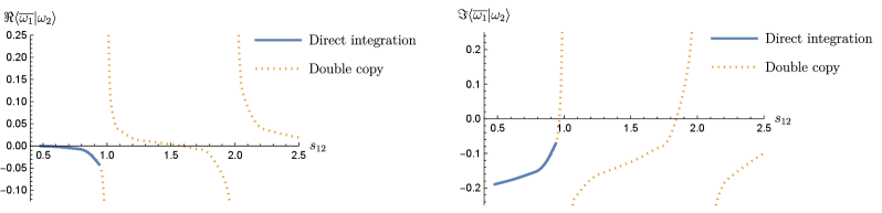
Figure 8: Real and imaginary values for the complex hypergeometric integral $\langle\overline{\omega}_{1}|\omega_{2}\rangle=J^{(g=2)}(z_{j},s_{ij})$. In blue, we plot the values obtained by direct integration, i.e. by performing the integral on the volume of $\Sigma_{2}^{*}$. In dashed orange lines we plot the values obtained by using the double copy formula. See the text for the values of the punctures and the moduli of $\Sigma_{2}^{*}$.

7.2 A double copy formula with a genus-two polylog kernel

In this example, our goal is to exemplify a double copy for the integral

$$J^{(g=2)}_{\textrm{polylog}}(z_{j},s_{ij}):=\int_{\Sigma_{2}^{*}} {\tilde{f}^{1}}_{\;\,2}(z_{1})\wedge\overline{\omega_{1}}\,\exp\big[s_{12}G(z_{1},z_{2})-s_{12}G(z_{1},z_{3})\big]\,,$$ (155)

where ${{\tilde{f}}^{1}}_{\;\,2}$ is a single-valued, bounded and non-holomorphic 1-form on $\Sigma_{2}$ given by the combination

$${\tilde{f}^{1}}_{\;\,2}(z_{1})={g^{1}}_{2}(z_{1})+2\pi i\,\omega_{2}(z_{1})\sum_{J=1}^{2}Y^{1J}\Im(\nu_{J}(z_{1}))\,.$$ (156)

This 1-form is readily obtained by taking the $\alpha_{1}$ coefficient of $\alpha_{2}\Omega_{2}(z_{1},z_{2},\alpha_{I})$, where $\Omega_{2}(z_{1},z_{2},\alpha_{I})$ is the single-valued Abelian Kronecker form (144), whose first few coefficients are:

$$\alpha_{2}\Omega_{2}(z_{1},z_{2},\alpha_{I}) =\omega_{2}+\alpha_{2}\,\bigg[{{g^{2}}_{2}(z_{1},z_{2})+2\pi i\omega_{2}\sum_{J=1}^{2}Y^{2J}\Im(\nu_{J}(z_{1}))}\bigg]$$

$$\phantom{=}+\alpha_{1}\bigg[{{g^{1}}_{2}(z_{1})+2\pi i\omega_{2}\sum_{J=1}^{2}Y^{1J}\Im(\nu_{J}(z_{1}))}\bigg]+\mathcal{O}(\alpha_{I}^{2})\,.$$ (157)

Therefore, we obtain a formula for $J^{(g=2)}_{\textrm{polylog}}(z_{j},s_{ij})$ from $J^{(g=2)}(z_{j},s_{ij},\alpha_{I})$, by isolating the $\overline{\alpha}_{1}^{0}\overline{\alpha}_{2}^{0}\alpha_{1}^{1}\alpha_{2}^{0}$-coefficient of

$$J^{(g=2)}(z_{j},s_{ij}.\alpha_{I})=\overline{\alpha}_{1}\alpha_{2}\int_{\Sigma_{2}^{*}}\Omega_{2}(z_{1},z_{2},\alpha_{I})\wedge\overline{\Omega_{1}(z_{1},z_{2},\alpha_{I})}\,\exp[s_{12}G(z_{1},z_{2})-s_{12}G(z_{1},z_{3})]\,.$$ (158)

We have already derived a general double-copy formula for the integral in the right-hand-side of (158): equation (6.3). For this double copy, we need the flowing vectors of integrals

$$\mathbf{I}_{1}^{(\alpha_{I},g=2)}=\begin{pmatrix}\int_{\gamma_{2A_{1}}}T(z_{1})\,F_{1}(z_{1},z_{2},\alpha_{I})\\ \int_{\gamma_{2B_{1}}}T(z_{1})\,F_{1}(z_{1},z_{2},\alpha_{I})\\ \int_{\gamma_{2A_{2}}}T(z_{1})\,F_{1}(z_{1},z_{2},\alpha_{I})\\ \int_{\gamma_{2B_{2}}}T(z_{1})\,F_{1}(z_{1},z_{2},\alpha_{I})\end{pmatrix} \mathbf{I}_{2}^{(\alpha_{I},g=2)}=\begin{pmatrix}\int_{\gamma_{2A_{1}}}T(z_{1})\,F_{2}(z_{1},z_{2},\alpha_{I})\\ \int_{\gamma_{2B_{1}}}T(z_{1})\,F_{2}(z_{1},z_{2},\alpha_{I})\\ \int_{\gamma_{2A_{2}}}T(z_{1})\,F_{2}(z_{1},z_{2},\alpha_{I})\\ \int_{\gamma_{2B_{2}}}T(z_{1})\,F_{2}(z_{1},z_{2},\alpha_{I})\,,\end{pmatrix}$$ (159)

where the $F_{J}(z_{1},z_{2},\alpha_{I})$ are Abelian Kronecker forms; see (144). Note that we understand these integrals formally, as generating functions, where the $\alpha_{I}$ are seen as expansion parameters (and affected by complex conjugation). Then, the double copy of (158) is

$$J^{(g=2)}(z_{j},s_{ij},\alpha_{I}) =\overline{\alpha}_{1}\alpha_{2}\exp\bigg[-2\pi\sum_{j=2}^{3}\ s_{1j}\sum_{I,J=1}^{2}Y^{IJ}\Im[\nu_{I}(z_{j})]\Im[\nu_{J}(z_{j})]\bigg]$$

$$\phantom{=}\times\big[{\mathbf{I}_{2}^{(\alpha_{I},g=2)}}\big]^{T}[\mathbf{H}^{2,2}_{\boldsymbol{\alpha}}]^{-1}\overline{{\mathbf{I}_{1}^{(\alpha_{I},g=2)}}}\bigg|_{\eqref{eq:substitution_rules_example}}\,$$ (160)

where $\mathbf{H}^{2,2}_{\boldsymbol{\alpha}}$, $\mathbf{I}_{a=1,2}^{(\alpha_{I},g=2)}$ are obtained from $\mathbf{H}^{2,2}$ (c.f., (7.1)) and $\mathbf{I}_{2}^{(g=2)}$ using the substitution rule $s_{1B_{I}}\to s_{1B_{I}}-\alpha_{I}$ (equation (131)). Then we set $s_{1B_{I}}$ as in equation (25), and make the substitution

$$s_{1A_{I}} \rightarrow\frac{1}{2i}\sum_{J=1}^{2}Y^{IJ}(\alpha_{J}-\overline{\alpha}_{J})-\sum_{J=1}^{2}Y^{IJ}s_{12}\Im\big[\nu_{J}(z_{2})-\nu_{J}(z_{3})\big]\,.$$ (161)

This substitution rule ensures that the $s_{1B_{J}}$ are self-conjugate.

Finally, the double copy of $J^{(g=2)}_{\textrm{polylog}}(z_{j},s_{ij})$, is given by taking the corresponding coefficient of $J^{(g=2)}$:

$$J^{(g=2)}_{\textrm{polylog}}(z_{j},s_{ij})=\overline{\alpha}_{1}^{0}\overline{\alpha}_{2}^{0}\alpha_{1}^{1}\alpha_{2}^{0}\textrm{-coefficient of }\eqref{eq:polylog_double_copy_example}\,.$$ (162)

We remark that this last formula is just a relation among integrals, and there is no $\alpha_{I}$-dependence in it. It simply is a double-copy formula for an integral of a single-valued, non-holomorphic and bounded $g=2$ polylogarithm kernel ${\tilde{f}^{1}}_{\;\,2}(z_{1})$, which we defined in equation (156). See ancillary file for a numeric verification of (162).

8 Conclusion and future directions

In this work, we have presented two families of hypergeometric functions on punctured Riemann surfaces of genus $g$, whose linear and quadratic relations – monodromy relations and double copy relations in physics parlance – follow from twisted homology and cohomology. More precisely, we present concrete examples of integrals that arise from pairing certain genus-$g$ twisted cohomology (introduced by Watanabe watanabe2016twisted ) and homology groups (introduced in this work). Exploiting pairings between these and closely related twisted (co)homology groups, this work culminates in a double copy formula for these families of genus-$g$ hypergeometric functions. This double copy is verified numerically using recently developed techniques crowdy2007computing ; crowdy2016schottky .

The hypergeometric integrals introduced in this work are natural generalizations of genus-one integrals known as Riemann-Wirtinger integrals Mano2012 . These integrals come in two flavors: either associated to single-valued differential forms or $\boldsymbol{\alpha}$-quasiperiodic Abelian Kronecker forms. The Kronecker form is a generating function in non-commutative variables for the so-called Enriquez integration kernels of genus-$g$ polylogarithms enriquez2021construction ; DHoker:2023vax ; Baune:2024biq . In particular, the double copy for certain symmetric linear combinations of higher-genus polylogarithms follows from the double copy of the $\boldsymbol{\alpha}$-quasiperiodic hypergeometric integrals introduced in this work.

We limit the scope to Abelian Kronecker forms in order to have a rank-1 local system; a homomorphism $\rho:\pi_{1}(\Sigma_{g}^{*},*)\rightarrow U(1)$. This is because the rank $r=1$ case is well studied and we have computational control over the web of pairings in figure 7 that lead to the twisted Riemann bilinear relations and the double copy. We expect that a better understanding of twisted (co)homology for rank $r>1$ will facilitate the double copy of (non-Abelian) Kronecker forms. This would extend the applicability of twisted (co)homology and the double copy to a wider array of higher genus polylogarithm kernels which are finding more and more applications in string theory DHoker:2025jgb , and hopefully will find application in quantum field theory. Perhaps the recent discovery of a double copy for string amplitudes in Anti-de Sitter spacetimes (Alday:2025bjp, , equation (1.10)) offers a physically well-motivated starting point for investigating twisted (co)homology of higher rank local systems.

Another physical motivation for understanding the twisted (co)homology of higher rank local systems is to provide a twisted (co)homology framework that more closely describes higher-genus string integrals – where two or more punctures are integrated over. We have limited the integrals in this work to one-fold integrals over a punctured genus-$g$ Riemann surface $\Sigma_{g}^{*}$. But in order to compute string amplitudes at $g$-loops, we need to integrate over the configuration space of $n$-punctures on a genus $g$ surface: $\operatorname{Conf}(n,\Sigma_{g})$. At genus-one, such integrals have been shown to involve local systems of rank $r>1$ (bhardwaj2024double, , section 7). The double copy relations on $\operatorname{Conf}(n,\Sigma_{g})$ would have a physical interpretation of “$g$-loop KLT relations”. See Stieberger:2022lss ; Stieberger:2023nol for examples of 1-loop KLT relations in the literature. Tantalizingly, recent work by Mazloumi and Stieberger Mazloumi:2024wys manages to relate the 1-loop KLT relations in Stieberger:2022lss ; Stieberger:2023nol to the double-copy of Riemann-Wirtinger integrals. In light of this, we hope that the methods of Mazloumi:2024wys could point directly to $g$-loop KLT relations, starting from the double copy studied here.

This work has also benefited from the numerical methods of Crowdy and Marshall crowdy2007computing ; crowdy2016schottky to evaluate functions and integrals on a punctured Riemann surface $\Sigma_{g}^{*}$. In this work, we have also extended these methods to evaluate the kernels of higher-genus polylogs. In the ancillary files, we share our numerical implementation, which includes the first publicly available implementation for the evaluation of a genus-two polylogarithmic kernel, namely ${g^{1}}_{2}(z_{1})$. We remark that the numerical method used here is conceptually different from the one described in Baune:2024biq ; SchottkyTools even though both rely on Schottky uniformization. It would be interesting to see how these methods compare in the numerical evaluation of the higher-genus polylogarithms and their special values (for example, the higher-genus multiple zeta values recently introduced in Baune:2025sfy ). We leave these comparisons for future work.

Appendix A Computation of homology intersection numbers

Here, we briefly describe a minimal set of homology intersection numbers so that, using the duality relations of equation (68), one can write down all the intersection numbers in equations (69) to (75). In writing down the intersection numbers, we use the common convention that a homology intersection number $[\gamma_{a}|\check{\gamma_{b}}]$ is written as sum of terms, where each term has three factors: (1) The coefficient in each $1$-chain $\Delta$ (for example, the factor $(e^{2\pi is_{1j}}-1)^{-1}$ in $[\gamma_{2j}]$). (2) Phases coming from comparing loadings – i.e. crossing branch cuts. And (3) a factor of $\pm 1$ coming form the relative orientation of each intersection.

In every computation here, we compute homology intersection numbers using unregularized contours in the second entry.

A.1 Intersection numbers involving $[\gamma_{2j}]$

There are three types of intersection numbers involving $[\gamma_{2j}]$: $[\gamma_{2j}|\check{\gamma}_{2k}]$, $[\gamma_{2A_{I}}|\check{\gamma}_{2j}]$, and $[\gamma_{2B_{I}}|\check{\gamma}_{2j}]$. The unregularized and regularized cycles are depicted in figure 3.

The intersection numbers $[\gamma_{2j}|\check{\gamma}_{2k}]$ are the simplest and have been computed before in many contexts. For example, Ghazouani-Pirio and Goto compute these at genus-one ghazouani2016moduli ; Goto2022 and are the same for any genus $g$. Conceptually, the fact we can reuse these intersection numbers from the genus-one case comes from the branch cuts being short. That is, the branch cuts fit inside a $4g$-gon as in figure 3.

For each pair $(j,k)$ with $j,k\in\{3,\dots,n-1\}$, the contours $\check{\gamma}_{2k}$ can be deformed such that $\gamma_{2j}$ and $\check{\gamma}_{2k}$ intersect at one point if $k<j$ and two points if $k\geq j$. By deforming $\check{\gamma}_{2k}$, one can ensure that it intersects $m_{0}\subset\gamma_{2j}$ below the branch cut for all $j$ and $k$. This intersection point contributes the term $\left((e^{2\pi is_{12}}-1)^{-1}\right)\cdot(1)\cdot(1)$ and is universal to all pairs $(j,k)$. Similarly, we choose $\check{\gamma}_{2k}$ such that it does not intersect $\ell_{2j}\subset\gamma_{2j}$ when $j>k$. With these conventions, $\check{\gamma}_{2k}$ also intersects $s_{j}\subset\gamma_{2j}$ when $j=k$ and contributes the term $\left(-(e^{2\pi is_{1k}}-1)^{-1}\right)\cdot(e^{2\pi is_{1k}})\cdot(-1)$. When $k>j$, $\check{\gamma}_{2k}$ also intersects $\ell_{2j}\subset\gamma_{2j}$ and contributes a term $(1)\cdot(1)\cdot(1)$ Putting this all together, one finds

$$[\gamma_{2j}|\check{\gamma}_{2k}]=\begin{cases}-\dfrac{e^{2\pi is_{12}}}{e^{2\pi is_{12}}-1}\,,&j<k\,,\\ -\dfrac{e^{2\pi i(s_{12}+s_{1j})}-1}{(e^{2\pi is_{12}}-1)(e^{2\pi is_{1j}}-1)}\,,&j=k\,,\\ -\dfrac{1}{e^{2\pi is_{12}}-1}\,,&j>k\,,\end{cases}$$ (163)

These intersection numbers $[\gamma_{2j}|\check{\gamma}_{2k}]$ agree with Goto2022 and (bhardwaj2024double, , equation (5.19)).

The intersection numbers $[\gamma_{2A_{I}}|\check{\gamma}_{2j}]$ and $[\gamma_{2A_{J}}|\check{\gamma}_{2j}]$ are new for $g>1$. Again, we deform $[\check{\gamma}_{2j}]$ so that it intersects the 1-chain $m_{0}$ but never $\ell_{A_{I}}\subset\gamma_{2A_{I}}$ or $\ell_{B_{I}}\subset\gamma_{2B_{I}}$. In both cases, the intersection number is solely generated by the intersection with $m_{0}$:

$$[\gamma_{2A_{I}}|\check{\gamma}_{2j}]=\left(\frac{1-e^{2\pi is_{1A_{I}}}}{e^{2\pi is_{12}}-1}\right)\cdot(1)\cdot(-1)\,.$$ (164)

$$[\gamma_{2B_{I}}|\check{\gamma}_{2j}]=\left(\frac{1-e^{2\pi is_{1B_{I}}}}{e^{2\pi is_{12}}-1}\right)\cdot(1)\cdot(-1)\,.$$ (165)

Up to the sign coming from relative orientation, these intersection numbers are simply the $m_{0}$ coefficient in $[\gamma_{2A_{I}}]$ or $[\gamma_{2B_{I}}]$ (c.f., (4.2)).

A.2 Intersection numbers involving $[\gamma_{2A_{I}}]$, $[\gamma_{2B_{J}}]$, with $I=J$

While these are genuinely new homology intersection numbers, they are easy to compute because the genus-one results can be recycled.

We will refer to the genus-one case of the local system simply by $s_{1A}$ and $s_{1B}$. Similarly, we denote the genus-one intersection numbers by, $[\gamma_{2A}|\check{\gamma}_{2B}]$, $[\gamma_{2A},\check{\gamma}_{2A}]$ and $[\gamma_{2B}|\check{\gamma}_{2B}]$. i.e. the $g=1$ $[\gamma_{2A_{1}}|\check{\gamma}_{2B_{1}}]=[\gamma_{2A}|\check{\gamma}_{2B}]$. Then, we claim:

$$[\gamma_{2A_{I}}|\check{\gamma}_{2B_{I}}] =[\gamma_{2A}|\check{\gamma}_{2B}]\big|_{(s_{1A},s_{1B})\rightarrow(s_{1A_{I}},s_{1B_{I}})}\,\,,$$

$$[\gamma_{2A_{I}}|\check{\gamma}_{2A_{I}}] =[\gamma_{2A}|\check{\gamma}_{2A}]\big|_{s_{1A}\rightarrow s_{1A_{I}}}\,\,,$$

$$[\gamma_{2B_{I}}|\check{\gamma}_{2B_{I}}] =[\gamma_{2B}|\check{\gamma}_{2B}]\big|_{s_{1B}\rightarrow s_{1B_{I}}}\,\,,$$ (166)

where we are using the notation $f(x)\big|_{x\rightarrow y}$ to stand for $f(y)$, i.e. replace the $x$ to $y$ in such expression.

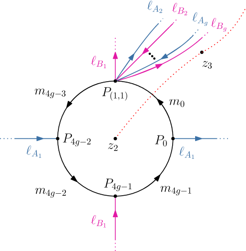
Figure 9: When computing the intersection numbers involving $[\gamma_{2A_{1}}]$ and $[\gamma_{2B_{1}}]$ only, we can use the following configuration, which resembles the genus-one case. We have collapsed all the $1$-simplices $m_{1},m_{2},\ldots,m_{4g-4}$ to the point $P_{(1,1)}$.

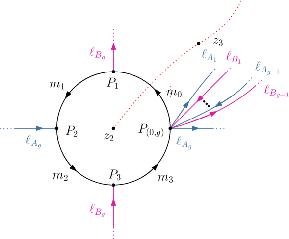
Figure 10: When computing the intersection numbers involving $[\gamma_{2A_{g}}]$ and $[\gamma_{2B_{g}}]$ only, we can use the following configuration, which resembles the genus-one case. We have collapsed all the $1$-simplices $m_{4},m_{5},\ldots,m_{4g-1}$ to the point $P_{(0,g)}$.

This is simplest to prove for $I=1$. The main idea is that when computing $[\gamma_{2A_{1}}|\check{\gamma}_{2B_{1}}]$ we could just squeeze all the 1-simplices $m_{1},m_{2},\ldots,m_{4g-4}$ to a point $P_{(1,1)}$. Then, all the cycles $\ell_{A_{I}}$, $\ell_{B_{I}}$, for $I=2,3,\ldots,g$ now all start and end at $P_{(1,1)}$. But now, we obtain a picture of the 1-simplices relevant to the genus-$g$ intersection number $[\gamma_{2A_{1}}|\check{\gamma}_{2B_{1}}]$ that looks just like the genus-one case. See figure 9. The case $I=g$ is proved in a similar way: for $I=g$, we instead collapse the 1-simplices $m_{4},m_{5},\ldots,m_{4g-1}$ to a point we call $P_{(0,g)}$. See figure 10.

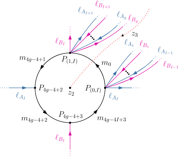
Figure 11: When computing the intersection numbers involving $[\gamma_{2A_{I}}]$ and $[\gamma_{2B_{I}}]$ only, $1<I<g$, we can use the following configuration, which resembles the genus-one case. We have collapsed all the $1$-simplices $m_{4},m_{5},\ldots,m_{4g-4I}$ to the point $P_{(1,I)}$. We have collapsed all the $1$-simplices $m_{4g-4I+4},m_{4g-4I+5},\ldots,m_{4g-1}$ to the point $P_{(0,I)}$.

For $1<I<g$, if we want to use this argument, we need to collapse the $1$-simplices $m_{4},m_{5},\ldots,m_{4g-4I}$ to a point, which we call $P_{(1,I)}$. Then we also collapse the $1$-simplices $m_{4g-4I+4},m_{4g-4I+5},\ldots,m_{4g-1}$ to a point we call $P_{(0,I)}$. The remaining $1$-simplices involved in the computation of any of the intersection numbers in our class are then in the configuration shown in figure 11. We see this resembles precisely the genus-one case, and thus our claim follows.

A.3 Intersection numbers involving $[\gamma_{2A_{I}}]$, $[\gamma_{2B_{J}}]$, with $I\neq J$

These are genuinely new homology intersection numbers that cannot be obtained from the genus-one results. Still they are straightforward to compute.

We remark that the unregulated cycles $\tilde{\gamma}_{2A_{I}}$ and $\tilde{\gamma}_{2B_{I}}$, $I=1,\ldots,g$ only intersect at $z_{2}$, and nowhere else on $\Sigma_{g}^{*}$. Moreover, we note that the unregulated cycles $[\tilde{\gamma}_{2\bullet_{I}}]$, $\bullet\in\{A,B\}$ can be deformed so that they intersect only $m_{4I-4+2}$ (in exactly 2 points: one ingoing and one outgoing). Thus, there are 2 summands in these homology intersection numbers, and we just need to compute them.

Also note that, for $I<J$, we only need to compute four homology intersection numbers here: $[\gamma_{2A_{I}}|\gamma_{2A_{J}}]$, $[\gamma_{2A_{I}}|\gamma_{2B_{J}}]$, $[\gamma_{2B_{I}}|\gamma_{2A_{J}}]$, $[\gamma_{2B_{I}}|\gamma_{2B_{J}}]$. The cases when $I>J$ are determined from equation (68) and the $I<J$ intersection numbers.

For reproducibility, we present the computation of $[\gamma_{A_{I}}|\check{\gamma}_{A_{J}}]$ in some more detail. We use a regularized cycle for $[\gamma_{A_{I}}]$ and an unregularized cycle for $[\check{\gamma}_{A_{J}}]$. Also recall that we deform $[\check{\gamma}_{A_{J}}]$ such that there are two points, $x$ and $y$ on $m_{4J-4+2}$ where $[\check{\gamma}_{A_{J}}]$ and $[\gamma_{A_{I}}]$ intersect. At $x$ let $[\check{\gamma}_{A_{J}}]$ be outgoing from $z_{2}$, and at $y$ let $[\check{\gamma}_{A_{J}}]$ be incoming towards $z_{2}$. Thus, the orientation at $x$ contributes a ($+1$) and the orientation at $y$ contributes a ($-1$). Similarly, the phases from crossing branch cuts at $x$ contribute $1$, and the phase from crossing branch cuts at $y$ contribute a factor of $e^{-2\pi is_{1A_{J}}}$. The remaining factor is the coefficient of the $m_{4J-4+2}$ 1-simplex in the regularized cycle $[\gamma_{2A_{I}}]$. From (4.2), this coefficient is $e^{2\pi is_{12}}\dfrac{1-e^{2\pi is_{1A_{I}}}}{e^{2\pi is_{12}}-1}$. Putting everything together yields:

$$[\gamma_{A_{I}}|\check{\gamma}_{A_{J}}] =\left(e^{2\pi is_{12}}\frac{1-e^{2\pi is_{1A_{I}}}}{e^{2\pi is_{12}}-1}\right)\cdot(1)\cdot(1)+\left(e^{2\pi is_{12}}\frac{1-e^{2\pi is_{1A_{I}}}}{e^{2\pi is_{12}}-1}\right)\cdot(e^{-2\pi is_{1A_{J}}})\cdot(-1)\,$$

$$=\frac{e^{2\pi is_{12}}\left(1-e^{2\pi is_{1A_{I}}}\right)\left(1-e^{-2\pi is_{1A_{J}}}\right)}{e^{2\pi is_{12}}-1}\,,\,\,\,I<J\,.$$ (167)

The hardest part of the procedure sketched above is having to find the coefficient of $m_{4g-4J+2}$ in the regularized cycles $\gamma_{2A_{I}}$ and $\gamma_{2B_{I}}$, for $I<J$. It turns out that this coefficient is always the same:

$$\textrm{Coefficient of }m_{{4g-4J+2}}\textrm{ in }\gamma_{2C_{I}}=e^{2\pi is_{12}}\dfrac{1-e^{2\pi is_{1A_{I}}}}{e^{2\pi is_{12}}-1}\,,\textrm{ for }C\in\{A,B\},\,\,I<J\,.$$ (168)

Further, note again that thanks to our convention in writing each summand in the first line of equation (A.3), we can read off how the factors therein reflect the paragraph above.

We conclude this section by listing the remaining three intersection numbers in a similar format:

$$[\gamma_{B_{I}}|\check{\gamma}_{A_{J}}] =\left(e^{2\pi is_{12}}\frac{1-e^{2\pi is_{1B_{I}}}}{e^{2\pi is_{12}}-1}\right)\cdot(1)\cdot(1)+\left(e^{2\pi is_{12}}\frac{1-e^{2\pi is_{1B_{I}}}}{e^{2\pi is_{12}}-1}\right)\cdot(e^{-2\pi is_{1A_{J}}})\cdot(-1)\,$$

$$=\frac{e^{2\pi is_{12}}\left(1-e^{2\pi is_{1B_{I}}}\right)\left(1-e^{-2\pi is_{1A_{J}}}\right)}{e^{2\pi is_{12}}-1}\,,\,\,\,I<J\,\,,$$ (169)

$$[\gamma_{B_{I}}|\check{\gamma}_{B_{J}}] =\left(e^{2\pi is_{12}}\frac{1-e^{2\pi is_{1B_{I}}}}{e^{2\pi is_{12}}-1}\right)\cdot(e^{-2\pi is_{1B_{J}}})\cdot(-1)+\left(e^{2\pi is_{12}}\frac{1-e^{2\pi is_{1B_{I}}}}{e^{2\pi is_{12}}-1}\right)\cdot(1)\cdot(1)\,$$

$$=\frac{e^{2\pi is_{12}}\left(1-e^{2\pi is_{1B_{I}}}\right)\left(1-e^{-2\pi is_{1B_{J}}}\right)}{e^{2\pi is_{12}}-1}\,,\,\,\,I<J\,\,,$$ (170)

$$[\gamma_{A_{I}}|\check{\gamma}_{B_{J}}] =\left(e^{2\pi is_{12}}\frac{1-e^{2\pi is_{1A_{I}}}}{e^{2\pi is_{12}}-1}\right)\cdot(e^{-2\pi is_{1B_{J}}})\cdot(-1)+\left(e^{2\pi is_{12}}\frac{1-e^{2\pi is_{1A_{I}}}}{e^{2\pi is_{12}}-1}\right)\cdot(1)\cdot(1)\,$$

$$=\frac{e^{2\pi is_{12}}\left(1-e^{2\pi is_{1A_{I}}}\right)\left(1-e^{-2\pi is_{1B_{J}}}\right)}{e^{2\pi is_{12}}-1}\,,\,\,\,I<J\,\,.$$ (171)

Appendix B Hypergeometric integrals in genus 1

Here, we focus on the case of hypergeometric integrals on a punctured genus-one Riemann surface. This appendix satisfies two purposes: We try to both study in particular the $g=1$ specialization of the genus-$g$ integrals (and twisted homology and cohomology groups) introduced in this work. Further, the functions involved in defining the $g=1$ hypergeometric integrals are more widely known, and as such the reader might refer to this section for some intuition and concreteness.

The genus-$1$ case of the hypergeometric integrals $I^{\varphi}_{\gamma}$ coincides precisely with the what the so-called Riemann-Wirtinger integrals Mano2012 ; ghazouani2016moduli ; Goto2022 ; bhardwaj2024double . Here, we will focus on how the twist function of the Riemann-Wirtinger integral coincides precisely with a $g=1$ version of the hypergeometric integrals here, and how the basis of twisted cohomology of Riemann-Wirtinger integrals also coincide with the cohomology bases here.

Let $\tau\in\mathbb{H}$ be the modulus of a torus in the upper-half plane, $\mathbb{H}={\{z\in\mathbb{C}|\Im z>0\}}$, and $E_{\tau}=\mathbb{C}/{(\mathbb{Z}+\tau\,\mathbb{Z})}$. Let $E_{\tau}^{*}=E_{\tau}-\{z_{2},\ldots,z_{n}\}$, where we have removed $(n-1)$ distinct punctures from $E_{\tau}$, and moreover $z_{2}=0$. The first homology of this genus-one Riemann surface, $H_{1}(E_{\tau})$ is of rank-2, generated by an $\mathfrak{A}$-cycle, corresponding to the cycle $\gamma_{2A}=z_{1}\in(0,1)$ and a $\mathfrak{B}$-cycle, corresponding to the cycle $\gamma_{2B}=z_{1}\in(0,\tau)$.

The odd Jacobi Theta function, $\theta_{1}:\mathbb{C}\times\mathbb{H}\rightarrow\mathbb{C}$, is defined by the series:

$$\theta_{1}(z,\tau)=-\sum_{m\in\mathbb{Z}}\exp\bigg(\pi i\left(m+\frac{1}{2}\right)^{2}\tau+2\pi i\left(m+\frac{1}{2}\right)\left(z+\frac{1}{2}\right)\bigg)\,,$$ (172)

which has the following quasiperiodicities:

$$\theta_{1}(z+1,\tau) =-\theta_{1}(z,\tau)\,$$ (173)

$$\theta_{1}(z+\tau,\tau) =-e^{\pi i(\tau+2z)}\theta_{1}(z,\tau)\,.$$ (174)

The theta function $\theta_{1}(z-x,\tau)$ will play the role of the prime function on $E_{\tau}$. Then, for $z_{1}\in E^{*}_{\tau}$, real numbers $s_{1A},s_{1j}$, $j=2,3,\ldots,n$ subject to $\sum_{j=2}^{n}s_{1j=0}$. We define the twist function of the Riemann-Wirtinger integral:

$$T_{RW}(z_{1})=\exp(2\pi is_{1A}z_{1})\,\prod_{j=2}^{n}\big[\theta_{1}(z_{1}-z_{j},\tau)\big]^{s_{1j}}\,.$$ (175)

Then the Riemann-Wirtinger integral, $I^{RW}$ takes the form:

$$I^{RW}=\int_{\gamma}T_{RW}(z_{1})\varphi_{RW}\,,$$ (176)

where the contours $\gamma$ are twisted cycles described in e.g. Fact 3.1 of Goto2022 and the $\varphi_{RW}\in H^{1}(E_{\tau},\nabla_{\omega_{RW}})$, i.e. they belong to the twisted cohomology group obtained form the twist $\omega_{RW}$:

$$\omega_{RW} =\text{d}_{z_{1}}\log T_{RW}(z_{1})\,$$

$$=2\pi is_{1A}\text{d}z_{1}+\sum_{j=2}^{n-1}[g^{(1)}(z_{1}-z_{j},\tau)-g^{(1)}(z_{1}-z_{n},\tau)]\text{d}z_{1}\,,$$ (177)

where $g^{(1)}(z,\tau)\text{d}z_{1}$ denotes the logarithmic differential of $\theta_{1}(z,\tau)$,

$$g^{(1)}(z,\tau)\,\text{d}z=\text{d}_{z}\log\theta_{1}(z,\tau)\,,$$ (178)

which has the quasiperiodicities

$$g^{(1)}(z+1,\tau) =g^{(1)}(z,\tau)\,$$

$$g^{(1)}(z+\tau,\tau) =g^{(1)}(z,\tau)-2\pi i\,,$$ (179)

and moreover $g^{(1)}(z,\tau)$ has a pole at $z=0$ of residue 1.

From this, we can infer that the terms $\big[g^{(1)}(z_{1}-z_{j},\tau)-g^{(1)}(z_{1}-z_{n},\tau)\text{d}z_{1}\big]$ appearing in the twist $\omega_{RW}$ are indeed meromorphic differentials of the third kind. Similarly, $\text{d}z_{1}$ is the unique holomorphic differential of first kind on $E_{\tau}$, so the formula for $\nabla_{RW}=\text{d}_{z_{1}}+\omega_{RW}$ is simply a genus-one version of the formula for the twist in (40), defined at any $g\geq 1$.

We similarly comment on the basis of twisted cohomology at genus-one, $H^{1}(E_{\tau},\nabla_{\omega_{RW}})$ which is generated by the one-forms Goto2022 :

$$H^{1}(E_{\tau},\nabla_{\omega_{RW}})=\operatorname{span}\bigg( \text{d}z_{1},\frac{\partial g^{(1)}}{\partial z_{1}}(z_{1}-z_{2},\tau)\text{d}z_{1},\big[g^{(1)}(z_{1}-z_{2},\tau)-g^{(1)}(z_{1}-z_{3},\tau)\big]\text{d}z_{1},$$

$$\big[g^{(1)}(z_{1}-z_{2},\tau)-g^{(1)}(z_{1}-z_{4},\tau)\big]\text{d}z_{1},\ldots,$$

$$\big[g^{(1)}(z_{1}-z_{2},\tau)-g^{(1)}(z_{1}-z_{n-1},\tau)\big]\text{d}z_{1}\bigg)\,.$$ (180)

This genus-$1$ basis of twisted cohomology coincides with the one at any genus, once we notice that $\frac{\partial g^{(1)}}{\partial z_{1}}(z_{1}-z_{2},\tau)\text{d}z_{1}$ is the unique (up to a holomorphic differential) meromorphic differential, doubly periodic, with a 2nd order pole at $z_{1}=z_{2}$, and that we can add together meromorphic differentials of third kind to obtain others:

$${\omega}(z_{1})_{z_{j},z_{k}}-{\omega}(z_{1})_{z_{k},z_{l}}={\omega}(z_{1})_{z_{j},z_{l}}\,,$$ (181)

and the linear relation in twisted cohomology:

$$[\omega_{RW}(z_{1})]\cong[0]\,,$$ (182)

which relates the holomorphic differential, $\text{d}z_{1}$ and the meromorphic differentials of third kind, ${\omega}(z_{1})_{z_{j},z_{k}}$.

The multivaluedness of the Riemann-Wirtinger twist along $\mathfrak{A}$- and $\mathfrak{B}$-cycles is given by:

$$T(z_{1}+\mathfrak{A}) =T(z_{1}+1)=e^{2\pi is_{1A}}T(z_{1})$$ (183)

$$T(z_{1}+\mathfrak{B}) =T(z_{1}+\tau)=e^{2\pi is_{1B}}T(z_{1})\,,$$ (184)

where $s_{1B}$ is given by:

$$s_{1B}=\tau s_{1A}+\sum_{j=2}^{n}s_{1j}z_{j}\,,$$ (185)

which is the genus-one version of (25).

With these definitions of $s_{1B}$ in mind, one can then proceed to compute regularized cycles in homology – see, e.g. section 3 of Mano2012 , compute homology intersection numbers – see, e.g. Proposition 3.4 of ghazouani2016moduli and obtain twisted Riemann bilinear relations, also known as double copy relations – see e.g. Proposition 4.22 of ghazouani2016moduli or equation (6.4) of bhardwaj2024double , which follows more closely our notation.

Appendix C Schottky uniformization and Numerical setup

In this work we deal with integrals of multivalued functions (times a 1-form) over Riemann punctured surfaces of genus $g$. We have found linear and quadratic relations among these integrals, all of which depend on many terms. As an internal check in our work, we have benefited from being able to numerically evaluate these integrals. Here, we will give a brief sketch of the numerical methods we have used – originally developed by Crowdy and Marshall crowdy2007computing – which use the setup of Schottky uniformization of a Riemann surface $\Sigma_{g}$. We will closely follow the presentation of crowdy2008geometric , and recommend the reader see the monograph crowdy2020solving for a pedagogical, detailed introduction.

Conceptually, Schottky uniformization allows us to give a model for a Riemann surface of genus $g$ starting from the Riemann sphere $\mathbb{CP}^{1}$, and using its complex structure. Consider $2g$ disjoint, non-nested circles on the Riemann sphere, which we will denote as Schottky circles, that come in pairs, $C_{1},C_{1}^{\prime},C_{2},C_{2}^{\prime},\ldots,C_{g},C_{g}^{\prime}$. Then, if we identify $C_{j}$ and $C_{j}^{\prime}$, for $j=1,2,\ldots,g$ in a continuous, one-to-one and orientation preserving way (i.e. a path going around $C_{j}$, with 1 turn in the counter-clockwise direction is mapped to a path going around $C_{j}^{\prime}$ in a clockwise direction, for 1 turn).

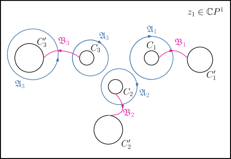
Figure 12: The exterior of the circles $C_{1},C_{1}^{\prime},C_{2},C_{2}^{\prime},C_{3},C_{3}^{\prime}$ is topologically a Riemann surface of genus-3. We draw also $\mathfrak{A}$- and $\mathfrak{B}$-cycles. The two blue cycles labeled $\mathfrak{A}_{3}$ are equivalent in homology – we draw them to emphasize their orientation.

After performing this identification, the exterior of the circles is topologically a compact Riemann surface of genus $g$, $\Sigma_{g}$. On this Riemann surface, we will identify the cycle homologous to $C_{j}$ with the $\mathfrak{A}_{j}$ cycle on $\Sigma_{g}$, and we identify a cycle going from one circle $C_{j}$ to the point on $C_{j}^{\prime}$ to which it is identified, by going along the exterior of the circle, as homologous to the $\mathfrak{B}_{j}$-cycle on $\Sigma_{g}$. See figure 12.

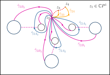
Figure 13: Integration cycles and branch cuts for $T(z_{1})$ for $z_{1}\in\Sigma_{g}$, for $(g,n)=(3,4)$. This corresponds to figure 2. Here, the dashed pink and blue (on the Schottky circles) lines correspond to the branch cuts of $T(z_{1})$ around $\mathfrak{A}$- and $\mathfrak{B}$-cycles.

There is more to Schottky uniformization than this topological identification of the exterior of these $2g$ circles to a Riemann surface $\Sigma_{g}$. We need more data: the data of a Schottky group $\Gamma\subset\operatorname{SL}(2,\mathbb{C})$, a subgroup of the groups of Möbius transformations. The way the circles $C_{j}$ and $C_{j}^{\prime}$ are identified with each other is by specifying a $f_{j}\in\operatorname{SL}(2,\mathbb{C})$ that maps the interior of $C_{j}$ into the exterior of $C_{j}^{\prime}$. Then, the Schottky group $\Gamma=\langle f_{1},f_{2},\ldots,f_{g}\rangle$ is freely generated by these generators and with a nonempty limit set, $\Lambda(\Gamma)$. Then the Riemann surface $\Sigma_{g}$ that is uniformized by $\Gamma$ is given by the quotient:

$$\Sigma_{g}=(\mathbb{CP}^{1}-\Lambda(\Gamma))/\Gamma\,.$$ (186)

More importantly, then, the exterior of the circles $C_{j},C_{j}^{\prime}$ are a fundamental domain for the Schottky group $\Gamma$, and this way we identify $\mathbb{CP}^{1}-\Lambda(\Gamma)$ as a cover for the Riemann surface $\Sigma_{g}$. In twisted (co)homology, we can work directly on the base space of our twist function $T(z_{1})$ rather than its cover, so its sufficient to work on the exterior of the Schottky circles. See figure 13. We remark Schottky uniformization is also convenient to understand the branch cuts of $T(z_{1})$.

The next crucial step is how to write nontrivial functions or forms on $\mathbb{CP}^{1}-\Lambda(\Gamma)$. These should be complex-valued functions which are, for example, automorphic with respect to the Schottky group elements:

$$\Phi(g\circ z)=\Phi(z)\,,\textrm{for }z\in\mathbb{CP}^{1}-\Lambda(\Gamma),g\in\Gamma\,.$$ (187)

equation (187) is a starting point to a theory of Poincaré series over $\Gamma$, out of which one can compute numerical approximations for holomorphic differentials $\omega_{j}$, prime functions $E(x,y)$ and even the kernels of polylogarithms ${g^{I}}_{J}(z_{1},z_{j})$ Baune:2024biq . But notice that if we want to compute functions or forms on $\Sigma_{g}$, we can try to focus on conditions only on the fundamental domain of the Schottky group (i.e. the exterior of the Schottky circles, including its boundary). This insight is the starting point for the Crowdy-Marshall method.

C.1 The Crowdy-Marshall method

The fundamental idea of the Crowdy-Marshall method is that we approximate a function (or form) in the exterior of the circles by rational approximation, and some logarithm terms as required. In the setup of crowdy2007computing , the Schottky group $\Gamma$ uniformizes a so-called $M$-curve, which implies that the period matrix $\Omega_{IJ}$ is purely imaginary for the corresponding Riemann surfaces. Then, in this setup one first obtains an approximation for the primitives of holomorphic differentials, $\nu_{J}(z_{1})$, $J=1,2,\ldots,g$, where the holomorphic differentials $\omega_{J}$ are normalized around the $\mathfrak{A}$-cycles. Because of this, if we denote $\delta_{j},\delta_{j}^{\prime}$ to be the centers of the Schottky circles $C_{j},C_{j}^{\prime}$, its multivaluedness in the exterior of the circles is given by a logarithm:

$$\nu_{j}(z_{1})=\frac{1}{2\pi i}\log\frac{z_{1}-\delta_{j}^{\prime}}{z_{1}-\delta_{j}}+r_{j}(z_{1}),$$ (188)

where $r_{j}(z_{1})$ is a rational function with poles inside the Schottky circles.

Then, these rational functions $r_{j}(z_{1})$ are given by some linear combinations:

$$r_{l}(z_{1})=\sum_{j=1}^{g}\sum_{n=1}^{N}\bigg[\frac{a_{l,j,n}}{(z_{1}-\delta_{j})^{n}}+\frac{b_{l,j,n}}{(z_{1}-\delta^{\prime}_{j})^{n}}\bigg]\,,l=1,2,\ldots,g\,,$$ (189)

and where the coefficients $a_{l,j,n}$ and $b_{l,j,n}$ above are determined from boundary conditions that $\nu_{j}(z_{1})$ satisfies. These boundary conditions are of the form:

$$\nu_{J}(z_{1})-\nu_{J}(h_{I}\circ z_{1})=\Omega_{IJ}\,,z_{1}\in C_{I}\,.$$ (190)

Then, one samples $N_{2}$ points on $C_{I}$, for $I=1,\ldots,g$, and uses linear regression to obtain approximations for the $a_{l,j,n}$ and $b_{l,j,n}$. This method is to give approximations for $\nu_{j}(z_{1})$ that get exponentially better as one increases $N_{1},N_{2}$, see e.g. the discussion on convergence rates in (trefethen2018series, , section 8), or (trefethen2024polynomial, , theorem 3).

Thus, by knowing some analytic properties of functions or forms (e.g. whether they have poles, residues along topological cycles, or whether they are single-valued or quasiperiodic on $\Sigma_{g}$) one can write corresponding functions and obtain similar approximations. Crowdy and Marshall do this too to obtain $E(z_{1},z_{j})$, the prime function (i.e. the components of the prime form).

These approximations are also particularly useful for numerically approximating the hypergeometric integrals $I^{\varphi}_{\gamma}$ because the form $T(z_{1})\varphi(z_{1})$ thus obtained is easy to evaluate and integrate.

C.2 A rational approximation for higher-genus polylogarithm kernels

One can similarly use the Crowdy-Marshall method, as explained above, to obtain approximations for the kernels of polylgarithms, ${g^{I_{1},_{I}2,\ldots,I_{r}}}_{J}(z_{1},z_{j})$ on the fundamental domain of the Schottky group $\Gamma$ – the exterior of the Schottky circles.

To give a concrete example, consider ${g^{1}}_{2}(z_{1})$. This is a 1-form given by (DHoker:2025dhv, , equation 6):

$${g^{1}}_{2}(z_{1})=\oint_{t\in\mathfrak{A_{1}}}\omega_{2}(t)\partial_{x}\log\frac{E(z_{1},z_{j})}{E(z_{1},t)}\,,z_{j}\in\Sigma_{g}\,,g\geq 2\,.$$ (191)

where this 1-form doesn’t depend on $z_{j}$.

Given that we know the quasiperiodicity and integrals around $\mathfrak{A_{J}}$-cycles of ${g^{1}}_{2}(z_{1})$, see equations (2) and (5), respectively, of DHoker:2025dhv , we can use the Crowdy-Marshall method to approximate it as a sum of rational functions, of the form of (189). The knowledge of the $\mathfrak{A_{J}}$-cycles periods of ${g^{1}}_{2}(z_{1})$ fixes the $a_{l,g,1}$, $b_{l,g,1}$ coefficients, and the knowledge of the quasiperiodicities gives us equations analogous to (190) for our linear system.

In supplementary material, we include a Mathematica implementation of the Crowdy-Marshall method, which we have checked against the Matlab implementation of crowdy2016schottky . We also include an implementation of the extension of this method for the Enriquez kernel ${g^{1}}_{2}(z_{1})$, included in ancillary files.

In the code, we include numerical checks of equations (4.1), (108) and (162).

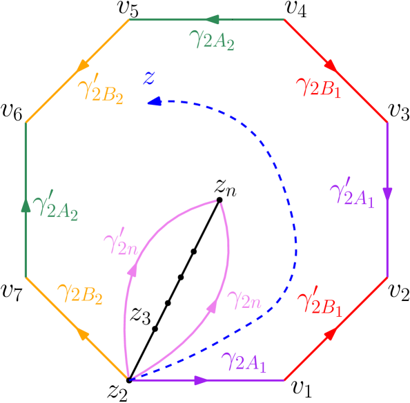
Figure 14: Structure of a genus-two surface as the $z_{1}$-space cut open to an octagon. The black lines denote the out choice of branch cut. The arrowed solid lines serve two purposes: on the one hand, the edges with the same color denote identified cycles, with the arrows specifying the orientation; on the other hand, they denote the integral paths (cycles) in equation (195), and those with the same color differ by a monodromy. The blue dashed line is the path to define the integral $\Omega(z)$ in equation (194): we always draw the path counter-clockwisely around the branch cut from $z_{2}$ to $z_{n}$.

Appendix D An elementary proof for the double copy relations

In this section, we will use Stokes theorem to derive the double copy relation on the integral over one variable. We employ the technique used by Ghazouani and Pirio in (ghazouani2016moduli, , Proposition 4.22) for the double copy relation at genus-one. Here we generalize there technique and give the explicit derivation for genus two, which is straightforward to generalize to higher genera.

We start with a complex hypergeometric integral over the genus-two Riemann surface $\Sigma_{2}^{*}$:

$$J_{2} =\int_{\Sigma_{2}^{*}}\xi(z_{1})\wedge\bar{\psi}(\bar{z}_{1})\,,$$ (192)

with

$$\bar{\psi}(z_{1}) =\bar{T}(z_{1})\bar{\phi}(z_{1})\,,$$ (193)

$$\xi(z_{1}) =T(z_{1})\phi(z_{1})\,.$$

Then, we define $\Xi(z)$ to be a local primitive of $\xi(z_{1})$:

$$\Xi(z):=\int_{z_{2}}^{z}\xi(z_{1})\,$$ (194)

where the integration path from $z_{2}$ to $z$ is taken along the dashed blue line in figure 14. Using Stokes theorem, we then have

$$J_{2} =\int_{\Sigma_{2}^{*}}\text{d}\Xi\wedge\bar{\psi}=\int_{\Sigma_{2}^{*}}\text{d}\big(\Xi\bar{\psi}\,\big)=\int_{\partial\Sigma_{2}}\Xi\,\bar{\psi}$$ (195)

$$=\left[\int_{\gamma_{2A_{1}}}-\int_{\gamma^{\prime}_{2A_{1}}}+\int_{\gamma^{\prime}_{2B_{1}}}-\int_{\gamma_{2B_{1}}}\right.\left.+\int_{\gamma_{2A_{2}}}-\int_{\gamma^{\prime}_{2A_{2}}}+\int_{\gamma^{\prime}_{2B_{2}}}-\int_{\gamma_{2B_{2}}}+\int_{\gamma^{\prime}_{2n}}-\int_{\gamma_{2n}}\right]\Xi\,\bar{\psi}\,,$$

where the contours listed above are given in figure 14. We compute the above summation separately according to the cycles. For the integrals over the $A_{1}$-cycle, we have:

$$\int_{z\in\gamma_{2A_{1}}}\bar{\psi}(\bar{z})\;{\color[rgb]{.5,0,.5}\Xi(z)}-\int_{z^{\prime}\in\gamma^{\prime}_{2A_{1}}}\bar{\psi}(\bar{z}^{\prime})\;{\color[rgb]{1,0,0}\Xi(z^{\prime})}$$ (196)

$$= \int_{z\in\gamma_{2A_{1}}}\bar{\psi}(z)\,{\color[rgb]{.5,0,.5}\left[\int_{z_{2}}^{z}\xi(z_{1})\right]}-\int_{z^{\prime}\in\gamma^{\prime}_{2A_{1}}}\bar{\psi}(z^{\prime})\,{\color[rgb]{1,0,0}\left[\int_{\gamma_{2A_{1}}+\gamma^{\prime}_{2B_{1}}-\gamma^{\prime}_{2A_{1}}}\xi(z_{1})+\int_{v_{3}}^{z^{\prime}}\xi(z_{1})\right]}\,.$$

Note that,

$$\int_{z\in\gamma_{2A_{1}}}\bar{\psi}(z)\,{\color[rgb]{.5,0,.5}\left[\int_{z_{2}}^{z}\xi(z_{1})\right]}=\int_{z^{\prime}\in\gamma^{\prime}_{2A_{1}}}\bar{\psi}(z^{\prime})\,{\color[rgb]{1,0,0}\left[\int_{v_{3}}^{z^{\prime}}\xi(z_{1})\right]}\,,$$ (197)

therefore we have

$$\int_{z\in\gamma_{2A_{1}}}\bar{\psi}(\bar{z})\,{\color[rgb]{.5,0,.5}\Xi(z)}-\int_{z^{\prime}\in\gamma^{\prime}_{2A_{1}}}\bar{\psi}(\bar{z}^{\prime})\,{\color[rgb]{1,0,0}\Xi(z^{\prime})}$$ (198)

$$= \,-\int_{z^{\prime}\in\gamma^{\prime}_{2A_{1}}}\bar{\psi}(z^{\prime})\,{\color[rgb]{1,0,0}\int_{\gamma_{2A_{1}}+\gamma^{\prime}_{2B_{1}}-\gamma^{\prime}_{2A_{1}}}\xi(z_{1})}$$

$$= \,e^{-2\pi is_{1B_{1}}}\bar{I}_{\gamma_{2A_{1}}}\Big[(e^{2\pi is_{1B_{1}}}-1)I_{\gamma_{2A_{1}}}-e^{2\pi is_{1A_{1}}}I_{\gamma_{2B_{1}}}\Big]\,.$$

Adding the contributions for the integrals over both $A_{J}$-cycles, we have

$$\int_{\gamma_{2A_{J}}}\bar{\psi}\,\Xi-\int_{\gamma^{\prime}_{2A_{J}}}\bar{\psi}\,\Xi$$ (199)

$$= \,e^{-2\pi is_{1B_{J}}}\bar{I}_{\gamma_{2A_{J}}}\Big[(e^{2\pi is_{1B_{J}}}-1)I_{\gamma_{2A_{J}}}-e^{2\pi is_{1A_{J}}}I_{\gamma_{2B_{J}}}\Big]\,,\quad J=1,2\,.$$

For integrals over $B_{J}$-cycles, we have

$$\int_{\gamma^{\prime}_{2B_{J}}}\bar{\psi}\,\Xi-\int_{\gamma_{2B_{J}}}\bar{\psi}\,\Xi$$ (200)

$$= \,\bar{I}_{\gamma_{2B_{J}}}\Big[(e^{-2\pi is_{1A_{J}}}+e^{2\pi is_{1B_{J}}}-1)I_{\gamma_{2A_{J}}}+(1-e^{2\pi is_{1A_{J}}})I_{\gamma_{2B_{J}}}\Big]\,,\quad J=1,2\,,$$

and finally, for integrals over $\gamma_{2n}$, we have

$$\int_{\gamma^{\prime}_{2n}}\bar{\psi}\,\Xi-\int_{\gamma_{2n}}\bar{\psi}\,\Xi$$ (201)

$$= \,\sum_{2\leqslant i\leqslant j<n}e^{-2\pi i(s_{12}+\cdots+s_{1i})}(1-e^{2\pi i(s_{12}+\cdots+s_{1j})})\bar{I}_{\gamma_{i,i+1}}I_{\gamma_{j,j+1}}$$

$$+\sum_{i=2}^{n-1}(e^{-2\pi i(s_{12}+\cdots+s_{1i})}-1)\bar{I}_{\gamma_{i,i+1}}I_{\gamma_{2,i}}\,,$$

where $\gamma_{i,i+1}=\gamma_{2,i+1}-\gamma_{2,i}$, for $i=3,4,\ldots,n-1$. Summing over equations (199), (200), and (201), we obtain the final formula for the double copy relation. One can also do these exercise at higher genus. The general double copy formula for arbitrary genus is:

$$\int_{\Sigma_{g}^{*}}T(z_{1})\overline{T(z_{1})}\,\phi(z_{1})\wedge\overline{\phi(z_{1})}$$ (202)

$$= \sum_{J=1}^{g}\,\bigg[(1-e^{-2\pi is_{1B_{J}}})I_{\gamma_{2A_{J}}}\bar{I}_{\gamma_{2A_{J}}}-e^{2\pi i(s_{1A_{J}}-s_{1B_{J}})}I_{\gamma_{2B_{J}}}\bar{I}_{\gamma_{2A_{J}}}$$

$$\qquad\ +(e^{-2\pi is_{1A_{J}}}+e^{2\pi is_{1B_{J}}}-1)I_{\gamma_{2A_{J}}}\bar{I}_{\gamma_{2B_{J}}}+(1-e^{2\pi is_{1A_{J}}})I_{\gamma_{2B_{J}}}\bar{I}_{\gamma_{2B_{J}}}\bigg]$$

$$+\sum_{1\leq J<K\leq g}\bigg[\big(1-e^{2\pi is_{1B_{J}}}\big)I_{\gamma_{2A_{J}}}-\big(1-e^{2\pi is_{1A_{J}}}\big)I_{\gamma_{B_{J}}}\bigg]\bigg[\big(1-e^{-2\pi is_{1B_{K}}}\big)I_{\gamma_{A_{K}}}-\big(1-e^{-2\pi is_{1A_{K}}}\big)I_{\gamma_{2B_{K}}}\bigg]$$

$$+\sum_{2\leq i\leq n-1}e^{-2\pi i(s_{12}+\cdots+s_{1i})}(1-e^{2\pi i(s_{12}+\cdots+s_{1j})})\bar{I}_{\gamma_{i,i+1}}I_{\gamma_{j,j+1}}$$

$$+\sum_{i=2}^{n-1}(e^{-2\pi i(s_{12}+\cdots+s_{1i})}-1)\bar{I}_{\gamma_{i,i+1}}I_{\gamma_{2,i}}\,,$$

with the path shown in figure 14. We have explicitly verified that the above formula coincides with the KLT kernel (7.1) used to build the double copy in (154) for $g=2$ and $n=3$ (once the $\gamma_{ij}$’s are written in terms of the basis of the main text).

References

- (1) S.-J. Matsubara-Heo, S. Mizera and S. Telen, Four lectures on Euler integrals, SciPost Phys. Lect. Notes 75 (2023) 1, [2306.13578].
- (2) D. A. Kosower, R. Monteiro and D. O’Connell, The SAGEX review on scattering amplitudes Chapter 14: Classical gravity from scattering amplitudes, J. Phys. A 55 (2022) 443015, [2203.13025].
- (3) A. Buonanno, M. Khalil, D. O’Connell, R. Roiban, M. P. Solon and M. Zeng, Snowmass White Paper: Gravitational Waves and Scattering Amplitudes, in Snowmass 2021, 4, 2022, 2204.05194.
- (4) K. Aomoto, M. Kita, T. Kohno and K. Iohara, Theory of hypergeometric functions. Springer, 2011.
- (5) M. Yoshida, Hypergeometric functions, my love: modular interpretations of configuration spaces, vol. 32. Springer Science & Business Media, 2013.
- (6) S. Mizera, Inverse of the String Theory KLT Kernel, JHEP 06 (2017) 084, [1610.04230].
- (7) S. Mizera, Combinatorics and Topology of Kawai-Lewellen-Tye Relations, JHEP 08 (2017) 097, [1706.08527].
- (8) S. Mizera, Scattering Amplitudes from Intersection Theory, Phys. Rev. Lett. 120 (2018) 141602, [1711.00469].
- (9) P. Mastrolia and S. Mizera, Feynman Integrals and Intersection Theory, JHEP 02 (2019) 139, [1810.03818].
- (10) S. Caron-Huot and A. Pokraka, Duals of Feynman integrals. Part I. Differential equations, JHEP 12 (2021) 045, [2104.06898].
- (11) S. Caron-Huot and A. Pokraka, Duals of Feynman Integrals. Part II. Generalized unitarity, JHEP 04 (2022) 078, [2112.00055].
- (12) F. Gasparotto, S. Weinzierl and X. Xu, Real time lattice correlation functions from differential equations, JHEP 06 (2023) 128, [2305.05447].
- (13) H. Frellesvig and T. Teschke, General relativity from intersection theory, Phys. Rev. D 110 (2024) 044028, [2404.11913].
- (14) C. Duhr, F. Porkert and S. F. Stawinski, Canonical differential equations beyond genus one, JHEP 02 (2025) 014, [2412.02300].
- (15) S. Stieberger, One-Loop Double Copy Relation in String Theory, Phys. Rev. Lett. 132 (2024) 191602, [2310.07755].
- (16) P. Mazloumi and S. Stieberger, One-loop double copy relation from twisted (co)homology, JHEP 10 (2024) 148, [2403.05208].
- (17) R. Bhardwaj, A. Pokraka, L. Ren and C. Rodriguez, A double copy from twisted (co)homology at genus one, JHEP 07 (2024) 040, [2312.02148].
- (18) Z. Bern, J. J. M. Carrasco, W.-M. Chen, H. Johansson, R. Roiban and M. Zeng, Five-loop four-point integrand of supergravity as a generalized double copy, Phys. Rev. D 96 (2017) 126012, [1708.06807].
- (19) V. S. Dotsenko and V. A. Fateev, Four Point Correlation Functions and the Operator Algebra in the Two-Dimensional Conformal Invariant Theories with the Central Charge c 1, Nucl. Phys. B 251 (1985) 691–734.
- (20) H. Kawai, D. C. Lewellen and S. H. H. Tye, A Relation Between Tree Amplitudes of Closed and Open Strings, Nucl. Phys. B 269 (1986) 1–23.
- (21) K. Aomoto, On the Complex Selberg Integral, The Quarterly Journal of Mathematics 38 (12, 1987) 385–399.
- (22) Z. Bern, J. J. M. Carrasco and H. Johansson, New Relations for Gauge-Theory Amplitudes, Phys. Rev. D 78 (2008) 085011, [0805.3993].
- (23) Z. Bern, J. J. Carrasco, M. Chiodaroli, H. Johansson and R. Roiban, The duality between color and kinematics and its applications, J. Phys. A 57 (2024) 333002, [1909.01358].
- (24) S. Stieberger, A Relation between One-Loop Amplitudes of Closed and Open Strings (One-Loop KLT Relation), 2212.06816.
- (25) T. Mano and H. Watanabe, Twisted cohomology and homology groups associated to the Riemann-Wirtinger integral, Proceedings of the American Mathematical Society 140 (2012) 3867–3881.
- (26) S. Ghazouani and L. Pirio, Moduli spaces of flat tori and elliptic hypergeometric functions, Mémoires de la Société mathématique de France (2016) , [1605.02356].
- (27) Y. Goto, Intersection numbers of twisted homology and cohomology groups associated to the Riemann-Wirtinger integral, International Journal of Mathematics 34 (June, 2022) 2350005, [2206.03177].
- (28) M. Hanamura and M. Yoshida, Hodge structure on twisted cohomologies and twisted Riemann inequalities I, Nagoya mathematical journal 154 (1999) 123–139.
- (29) H. Watanabe, Twisted cohomology of a punctured Riemann surface, Kumamoto J. Math. 29 (2016) 55–63.
- (30) K. Cho and K. Matsumoto, Intersection theory for twisted cohomologies and twisted Riemann’s period relations I, Nagoya Mathematical Journal 139 (1995) 67–86.
- (31) D. Bernard, On the Wess-Zumino-Witten models on Riemann surfaces, Nuclear Physics B 309 (1988) 145–174.
- (32) B. Enriquez, Flat connections on configuration spaces and braid groups of surfaces, Advances in Mathematics 252 (2014) 204–226, [1112.0864].
- (33) B. Enriquez and F. Zerbini, Construction of Maurer-Cartan elements over configuration spaces of curves, 2110.09341.
- (34) K. Baune, J. Broedel, E. Im, A. Lisitsyn and F. Zerbini, Schottky–Kronecker forms and hyperelliptic polylogarithms, J. Phys. A 57 (2024) 445202, [2406.10051].
- (35) A. Lisitsyn, Representations of Kronecker forms at higher genus, Master’s thesis, ETH Zürich, 2024.
- (36) E. D’Hoker, M. Hidding and O. Schlotterer, Constructing polylogarithms on higher-genus Riemann surfaces, Commun. Num. Theor. Phys. 19 (2025) 355–413, [2306.08644].
- (37) D. A. Hejhal, Theta functions, kernel functions and Abelian integrals, vol. 129. American Mathematical Soc., 1972.
- (38) E. D’Hoker and O. Schlotterer, Meromorphic higher-genus integration kernels via convolution over homology cycles, J. Phys. A 58 (2025) 33LT01, [2502.14769].
- (39) P. de Maat, “Twisted Cohomology and Feynman Integrals.” Master’s Thesis, Utrecht University, 2021.
- (40) E. Casali, S. Mizera and P. Tourkine, Monodromy relations from twisted homology, JHEP 12 (2019) 087, [1910.08514].
- (41) E. Casali, S. Mizera and P. Tourkine, Loop amplitudes monodromy relations and color-kinematics duality, JHEP 03 (2021) 048, [2005.05329].
- (42) K. Mimachi and M. Yoshida, Intersection numbers of twisted cycles and the correlation functions of the conformal field theory II, Commun. Math. Phys. 234 (2003) 339–358, [math/0208097].
- (43) K. Mimachi, K. Ohara and M. Yoshida, Intersection numbers for loaded cycles associated with Selberg-type integrals, Tohoku Mathematical Journal, Second Series 56 (2004) 531–551.
- (44) S. Mizera, Aspects of Scattering Amplitudes and Moduli Space Localization, Ph.D. thesis, Princeton, Inst. Advanced Study, 2020. 1906.02099. 10.1007/978-3-030-53010-5.
- (45) E. D’Hoker and D. H. Phong, The Geometry of String Perturbation Theory, Rev. Mod. Phys. 60 (1988) 917.
- (46) E. D’Hoker, C. R. Mafra, B. Pioline and O. Schlotterer, Two-loop superstring five-point amplitudes. Part I. Construction via chiral splitting and pure spinors, JHEP 08 (2020) 135, [2006.05270].
- (47) C. R. Mafra and O. Schlotterer, Towards the n-point one-loop superstring amplitude. Part II. Worldsheet functions and their duality to kinematics, JHEP 08 (2019) 091, [1812.10970].
- (48) J. Broedel, C. R. Mafra, N. Matthes and O. Schlotterer, Elliptic multiple zeta values and one-loop superstring amplitudes, JHEP 07 (2015) 112, [1412.5535].
- (49) E. D’Hoker, B. Enriquez, O. Schlotterer and F. Zerbini, Relating flat connections and polylogarithms on higher genus Riemann surfaces, 2501.07640.
- (50) D. G. Crowdy and J. S. Marshall, Computing the Schottky-Klein prime function on the Schottky double of planar domains, Computational Methods and Function Theory 7 (2007) 293–308.
- (51) D. Crowdy, E. Kropf, C. Green and M. Nasser, The schottky–klein prime function: a theoretical and computational tool for applications, IMA Journal of Applied Mathematics 81 (2016) 589–628.
- (52) E. D’Hoker and O. Schlotterer, Worldsheet fermion correlators, modular tensors and higher genus integration kernels, 2505.07947.
- (53) L. F. Alday, M. Nocchi and A. S. Sangaré, Stringy KLT Relations on , 2504.19973.
- (54) E. Im. SchottkyTools: Software package for numerical evaluation of higher-genus polylogarithms. Work in progress.
- (55) K. Baune, J. Broedel, E. Im, Z. Ji and Y. Moeckli, Higher-genus multiple zeta values, 2507.21765.
- (56) D. Crowdy, Geometric function theory: a modern view of a classical subject, Nonlinearity 21 (2008) T205.
- (57) D. Crowdy, Solving problems in multiply connected domains. SIAM, 2020.
- (58) M. Seppälä, Myrberg’s numerical uniformization of hyperelliptic curves, Annales Fennici Mathematici 29 (2004) 3–20.
- (59) L. N. Trefethen, Series solution of Laplace problems, The ANZIAM Journal 60 (2018) 1–26.
- (60) L. N. Trefethen, Polynomial and rational convergence rates for Laplace problems on planar domains, Proceedings of the Royal Society A 480 (2024) 20240178.
- (61) K. Baune, J. Broedel, E. Im, A. Lisitsyn and Y. Moeckli, Higher-genus Fay-like identities from meromorphic generating functions, SciPost Phys. 18 (2025) 093.