Statistics-Friendly Confidentiality Protection for Establishment Data, with Applications to the QCEW

Abstract.

Confidentiality for business datais an understudied area of disclosure avoidance, where legacy methods struggle to provide acceptable results. Modern formal privacy techniques designed for person-level data do not provide suitable confidentiality/utility trade-offs due to the highly skewed nature of business data and because extreme outlier records are often important contributors to query answers. In this paper, inspired by Gaussian Differential Privacy, we propose a novel confidentiality framework for business data with a focus on interpretability for policy makers. We propose two query-answering mechanisms and analyze new challenges that arise when noisy query answers are converted into confidentiality-preserving microdata. We evaluate our mechanisms on confidential Quarterly Census of Employment and Wages (QCEW) microdata and a public substitute dataset.

1. Introduction

Business data provide crucial snapshots of various sectors of a country’s economy. The collection and dissemination of business statistics is of great value in both the public and private sectors. As with person-level data, there are strong confidentiality concerns, but the requirements are not the same. Protections for person-level data are designed to mask records that are outliers, as individuals with uncommon characteristics can be vulnerable to disclosure and harassment. However, the “outliers” in business data are the large companies whose contributions to employment and wage statistics are important to study. In business data, the analogue to a person is an establishment, which is a single physical location where business activity occurs (e.g., a specific restaurant in a restaurant chain).Disclosure avoidance for person-level data has advanced with the rise of differential privacy (DP) (Dwork et al., 2006), but much less work has focused on protecting establishment data.The dominant methods in use are cell suppression (Adam and Worthmann, 1989) and EZS multiplicative noise (Evans et al., 1996), and to some extent synthetic data (Pistner et al., 2018; Kinney et al., 2011). Although currently used for the QCEW, cell suppression is complex, time-consuming, redacts significant amounts of data, and lacks composition – it can be reverse engineered when additional statistics are published. These are significant drawbacks for the QCEW, which (as we explain in Section 2) effectively has 54 different owners subject to different regulations and almost no coordination. While EZS noise enables the release of more statistics, it under-protects small establishments and distorts high-level aggregates, making it an nonviable option for QCEW (Yang et al., 2011b).Formal privacy for establishment data has so far received little attention (Haney et al., 2017; Seeman et al., 2024; Finley et al., 2024; Tran et al., 2023). The challenges include: interpretability for the mathematical statisticians and policy makers in statistical agencies; flexibility to customize the confidentiality-utility trade-off by allowing policy makers to specify how information leakage for large establishments should differ from leakage for small establishments (this flexibility is necessary because of the sparsity of establishment data and the presence of important outliers); statistics-friendliness requires noisy query answers to have relatively simple noise distributions for downstream analyses. Prior work (Haney et al., 2017; Seeman et al., 2024; Finley et al., 2024) based on concentrated DP (Bun and Steinke, 2016) make interpretation of confidentiality leakage difficult and often do not support a customizable confidentiality-utility trade-off (Haney et al., 2017; Seeman et al., 2024). More recent work (Finley et al., 2024) supports some flexibility, but either adds more noise to aggregate queries than needed (negatively impacting utility) or adds the same amount of noise to a tiny establishment as it does to a huge company (negatively impacting confidentiality). Another unaddressed concern is that the most natural confidentiality mechanisms for establishment data have data-dependent variances. We show this can introduce huge biases when converting noisy query answers into microdata. We analyze the impacts on utility through two metrics: the absolute error (the absolute difference between the sanitized value and the original value) and relative error (the absolute error over the original value).Our contributions are:

• We propose a confidentiality framework for establishment data that we call Gaussian Establishment Differential Privacy (referred to as Gaussian Establishment DP or gedp). It provides confidentiality guarantees directly in terms of uncertainty intervals and hypothesis tests, making it interpretable to mathematical statisticians and economists who typically help set policies in federal statistical agencies. We precisely characterize the class of functions (which we call “neighbor functions”) that can be used to specify how information leakage for large establishments should differ from small establishments.

• Most work on business data confidentiality focuses on protecting inference about establishments up to a certain amount of relative error. In a sharp break from tradition, we argue why such an approach is inadequate for utility and for confidentiality. We propose an alternative using the neighbor functions mentioned above.

• Microdata is often obtained from noisy query answers by solving a weighted least squares optimization problem (Li et al., 2015; Abowd et al., 2022). We demonstrate, mathematically and experimentally, how query-answering mechanisms with data-dependent variances (whose exact values cannot be released) impact this process. Specifically, we show how uncertainty about the true variance, combined with its data dependence, can introduce significant bias in microdata.

• We introduce two mechanisms for Gaussian Establishment DP, the $\psi$-mechanism and pnc-mechanism, to help combat this problem with microdata generation. The $\psi$-mechanism (which is similar to the transformation mechanisms of Finley et al. (Finley et al., 2024)) has data-dependent variance that cannot be revealed exactly. However, the pnc-mechanism piggybacks on top of the $\psi$-mechanism to provide query answers with data-dependent Gaussian noise whose variance can be released exactly. This makes it suitable for creating microdata out of the noisy query answers.

• We evaluate our mechanisms on real-world data (a historical, confidential QCEW dataset) and on a publicly shareable synthetic dataset that we generated from available U.S. Census datasets to mimic QCEW structure.

This paper is organized as follows. We provide background information on the QCEW in Section 2 since the design of formal privacy definitions for establishment data require an understanding of the confidentiality concerns and characteristics of such data. In Section 3, we present notation and technical background on Gaussian Differential Privacy (Dong et al., 2021) (which motivates our framework) and discuss related work in Section 4. In Section 5, we propose and carefully analyze the privacy definition Gaussian Establishment DP. We present two query-answering mechanisms in Section 6. In Section 7, we analyze the effects of data-dependent query noise variance on the synthetic data generation process. We present experiments on (confidential) real and (publicly available) partially synthetic data in Section 8. We conclude and outline future work in Section 9.

2. Background on the QCEW

The Bureau of Labor Statistics (BLS) Quarterly Censusof Employment and Wages (QCEW) data is an economically and politically important dataset containing wage and employment information about businesses in the United States.The data provided by QCEW are crucial for measuring labor trends and industry developments, provide a sample-frame for all BLS establishment surveys, and are used to benchmark the Current Employment Statistics survey, which is a primary economic indicator used by the federal reserve (Brave et al., 2021). QCEW data has also been used for a wide range of analyses that have helped economists understand the effects of minimum wage, the non-profit sector and the effect of the COVID-19 pandemic on employment levels (Meer and West, 2016; Salamon and Sokolowski, 2005; Dalton et al., 2020).

2.1. Data Collection, Schema and Dissemination

The QCEW is collected each quarter under a cooperative program between BLS and the State Employment Security Agencies.States collect the data from unemployment insurance (UI) administrative records which firms are legally obligated to submit quarterly. The primary unit of analysis is an establishment, which is a single physical location where one predominant activity, classified by a single industry code, occurs (Sadeghi et al., 2016). Meanwhile, a firm is a business made up of one or more establishments. All of the state-collected, administrative data, coveringover 10 million establishments, are sent to the BLS (U.S. Bureau of Labor Statistics, 2024a; Cohen and Li, 2006).Since the UI data are collected for all U.S. workers covered by state unemployment insurance laws or by the Unemployment Compensation for Federal Employees program, they represent a virtual census of employment and wages, providing a complete overview of the national economic picture.BLS supplements the states’ UI data collection by conducting an annual refiling survey to ensure each establishment is labeled under the correct industry code and further cleans the data. The data from each state are then sent back to the state along with BLS produced aggregated estimates protected by a disclosure limitation method. Each state retains ownership over its own data under this arrangement. Thus, there are 54 different data curators/publishers (50 states, the District of Columbia, Puerto Rico, Virgin Islands, and BLS), each covered by different laws and policies.Data Schema: Quarterly data about each establishment include (1) location (e.g., county and state), (2) total quarterly wages, (3) three monthly employment counts, (4) an ownership type (private, local government, etc.) and (5) a six-digit industry code known as the North American Industry Classification System (NAICS) code. The NAICS code (U.S. Census Bureau, 2024) is hierarchically structured. For example, “construction” has the NAICS prefix 23, “construction of buildings” has the prefix 236 and the NAICS code for “new multifamily housing construction” is 236116. The wages and employment data are considered confidential while the rest of the attributes (county, NAICS code, ownership type) are considered public.Dissemination: The QCEW establishment-level data are published in aggregated form, mostly as group-by sum queries, also known as marginals and are identified by an aggregation level code (U.S. Bureau of Labor Statistics, 2024b); e.g., aggregation level 15 (“National, by NAICS 3-digit – by ownership sector”) provides the national-level total quarterly wages and monthly employment totals for each combination of 3-digit NAICS code and ownership type (private, foreign government, state government, etc.) while aggregation level 55 provides the same information, but broken down by state, and 75 breaks it down by county.BLS also receives requests for custom tabulations. Thus a highly desirable property for a disclosure avoidance system is the ability to convert noisy query answers into confidentiality-protected microdata from which those custom tabulations can be computed.

2.2. Disclosure Avoidance

The BLS is obligated to use statistical disclosure limitation methods to protect sensitive values (employment and wages) of individual establishments. Internal policy and federal law, specifically the Confidential Information Protection and Statistical Efficiency Act (CIPSEA) of 2002, require confidentiality protections to all data acquired and maintained by the BLS under a pledge of confidentiality.The current disclosure avoidance method for the QCEW is cell suppression.According to the cell suppression methodology (Adam and Worthmann, 1989), sensitive cells are initially identified by either the $p\%$ rule, the $qp$-rule or the $nk$-rule (Schmutte and Vilhuber, 2020). The $p\%$ rule, for example, considers the question of whether the second largest establishment in a cell can use the cell total to learn the largest establishment’s confidential value up to $p\%$ relative error (a cell is flagged as sensitive if the cell total minus the contributions of the two largest establishments is less than $p\%$ of the largest establishment). These cells are suppressed in a step called primary suppression. The secondary suppression phase then identifies combinations of cells from which the suppressed cells can be deduced via linear algebra. This phase removes additional cells so that such combinations no longer exist.Primary and secondary suppression procedures result in the BLS suppressing the majority of the cells before they are released (U.S. Bureau of Labor Statistics, 2024a). Over 60% of more than 3.6 million cells in the QCEW tables are suppressed (Cohen and Li, 2006; Yang et al., 2011a; Toth, 2014). Apart from concerns about loss of data, secondary suppression can be complex to implement and often requires solving computationally expensive linear programs (Cox, 1980).Cell suppression also has two major confidentiality vulnerabilities. First, it is brittle against external knowledge –it is possible for, say Pennsylvania, to release additional data about its establishments that, when combined with cell-suppressed QCEW data, allows attackers to reverse engineer other cells (e.g., compromising confidentiality for businesses in New York). Second, cell suppression is only designed to protect against linear attackers – those who only use addition, subtraction, and scalar multiplication to attack data. It is not designed to protect against more sophisticated statistical attacks (Holan et al., 2010), which is why the $p$ parameter from the $p\%$ rule is also kept confidential. It is therefore not possible to realistically determine what confidential values might become vulnerable to disclosure when new types of data tabulations are published. This prevents the BLS from publishing new statistics and analyses from the QCEW microdata because of the unknown ways that new data products could impact the disclosure protections of existing products.

3. Notation and Background

Differential privacy (DP), as used for person data, does not provide suitable confidentiality/utility trade-off for protecting establishment data that are highly skewed by nature and extreme outlier records are key contributors to statistics of interest. The amount of noise needed to mask large establishments (such as those belonging to Disneyland Resort) would render many statistics unfit for use.Our framework for protecting establishment data extends DP by specifying how information leakage about large establishments should differ from small establishments. It is compatible with any version of DP that supports adaptive composition and additive noise. For this paper, we utilize Gaussian DP (Dong et al., 2021) because its semantics appeal to statisticians working at statistical government agencies.

Table 1. Table of Notation

$\Phi$:	Gaussian CDF
$\mu$:	Gaussian DP and gedp Privacy Parameter
${{\color[rgb]{0,0,0}\mathcal{E}}}$:	An establishment
${{\color[rgb]{0,0,0}n}}$:	Number of establishments
${{\color[rgb]{0,0,0}\mathcal{D}}}$:	Data set of records for establishments ${{\color[rgb]{0,0,0}\mathcal{E}}}_{1},\dots,{{\color[rgb]{0,0,0}\mathcal{E}}}_{{\color[rgb]{0,0,0}n}}$
${{\color[rgb]{0,0,0}A}}_{1},\dots,{{\color[rgb]{0,0,0}A}}_{{\color[rgb]{0,0,0}{{\color[rgb]{0,0,0}k}}_{p}}}$:	Public attributes of an establishment
${{\color[rgb]{0,0,0}C}}_{1},\dots,{{\color[rgb]{0,0,0}C}}_{{\color[rgb]{0,0,0}{{\color[rgb]{0,0,0}k}}_{c}}}$:	Confidential attributes of an establishment
${{\color[rgb]{0,0,0}r}}$:	Establishment record. ${{\color[rgb]{0,0,0}r}}[{{\color[rgb]{0,0,0}C}}_{i}]$ is the value for ${{\color[rgb]{0,0,0}C}}_{i}$
${{\color[rgb]{0,0,0}\psi}}$:	Neighbor function (Definition 5.1).
${{\color[rgb]{0,0,0}\gamma}}$:	Closeness parameter (Definition 5.1).
${{\color[rgb]{0,0,0}\mathcal{M}}}$:	Mechanism.
${{\color[rgb]{0,0,0}\mathcal{I}}}_{{{\color[rgb]{0,0,0}\psi}},{{\color[rgb]{0,0,0}\gamma}}}(x)$:	Uncertainty interval around $x$ induced by ${{\color[rgb]{0,0,0}\psi}},{{\color[rgb]{0,0,0}\gamma}}$.
${{\color[rgb]{0,0,0}gsum}}_{\langle{{\color[rgb]{0,0,0}\mathcal{G}}},{{\color[rgb]{0,0,0}C}}_{i}\rangle}$:	Group-by sum query over ${{\color[rgb]{0,0,0}C}}_{i}$ with grouper ${{\color[rgb]{0,0,0}\mathcal{G}}}$.

The notation used in the paper is summarized in Table 1.A dataset ${{\color[rgb]{0,0,0}\mathcal{D}}}$ contains records about establishments ${{\color[rgb]{0,0,0}\mathcal{E}}}_{1},\dots,{{\color[rgb]{0,0,0}\mathcal{E}}}_{{{\color[rgb]{0,0,0}n}}}$. Establishments have public attributes ${{\color[rgb]{0,0,0}A}}_{1},\dots,{{\color[rgb]{0,0,0}A}}_{{{\color[rgb]{0,0,0}{{\color[rgb]{0,0,0}k}}_{p}}}}$ and confidential attributes ${{\color[rgb]{0,0,0}C}}_{1},\dots,{{\color[rgb]{0,0,0}C}}_{{\color[rgb]{0,0,0}{{\color[rgb]{0,0,0}k}}_{c}}}$. The confidential attributes are numeric and nonnegative (e.g., number of employees). The nonnegativity condition is natural and, as we explain, is without loss of generality. First, sensitive establishment attributes are often aggregations of business operations (e.g., number of employees, total wages, etc.) that are intrinsically nonnegative. Second, even attributes that can be negative (like profit) can be incorporated in at least two ways:

• Sometimes an attribute can be naturally expressed as the difference of two nonnegative attributes; e.g., profit can be replaced by revenue and cost, since profit is the difference of the two.

• Otherwise, a confidential attribute ${{\color[rgb]{0,0,0}C}}$ that is sometimes negative can be replaced with ${{\color[rgb]{0,0,0}C}}^{\prime}=\max(0,{{\color[rgb]{0,0,0}C}})$ and ${{\color[rgb]{0,0,0}C}}^{{}^{\prime\prime}}=|\min(0,{{\color[rgb]{0,0,0}C}})|$. If ${{\color[rgb]{0,0,0}C}}$ is profit, ${{\color[rgb]{0,0,0}C}}^{\prime}$ can be interpreted as the gain and ${{\color[rgb]{0,0,0}C}}^{\prime\prime}$ can be interpreted as the loss. Both ${{\color[rgb]{0,0,0}C}}^{\prime}$ and ${{\color[rgb]{0,0,0}C}}^{\prime\prime}$ are nonnegative and ${{\color[rgb]{0,0,0}C}}={{\color[rgb]{0,0,0}C}}^{\prime}-{{\color[rgb]{0,0,0}C}}^{\prime\prime}$.

We use ${{\color[rgb]{0,0,0}a}}_{i}$ (resp., ${{\color[rgb]{0,0,0}c}}_{i}$) to refer to specific values of attribute ${{\color[rgb]{0,0,0}A}}_{i}$ (resp., ${{\color[rgb]{0,0,0}C}}_{i}$). Thus, we can represent an establishment record $r$ as a tuple ${{\color[rgb]{0,0,0}r}}=({{\color[rgb]{0,0,0}a}}_{1},\dots,{{\color[rgb]{0,0,0}a}}_{{\color[rgb]{0,0,0}{{\color[rgb]{0,0,0}k}}_{p}}},{{\color[rgb]{0,0,0}c}}_{1},\dots,{{\color[rgb]{0,0,0}c}}_{{{\color[rgb]{0,0,0}{{\color[rgb]{0,0,0}k}}_{c}}}})$ and refer to attributes within a record using indexing notation; e.g., the value of attribute ${{\color[rgb]{0,0,0}C}}_{1}$ in ${{\color[rgb]{0,0,0}r}}$ is ${{\color[rgb]{0,0,0}r}}[{{\color[rgb]{0,0,0}C}}_{1}]$.A mechanism ${{\color[rgb]{0,0,0}\mathcal{M}}}$ is a randomized algorithm whose input is confidential data and whose output is intended for public distribution.Let $\Phi$ denote the cumulative distribution function of the standard normal distribution.Gaussian DP (Dong et al., 2021) for person data is defined as:

Definition 3.1 ($f$-DP and $\mu$-Gaussian DP (Dong et al., 2021)).

Let $f$ be a continuous, concave, non-decreasing function such that $f(x)\geq x$. A mechanism ${{\color[rgb]{0,0,0}\mathcal{M}}}$ satisfies $f$-DP if for all pairs of datasets ${{\color[rgb]{0,0,0}\mathcal{D}}}_{1},{{\color[rgb]{0,0,0}\mathcal{D}}}_{2}$ that differ on the value of one record and for all $S\subseteq{{\color[rgb]{0,0,0}range}}({{\color[rgb]{0,0,0}\mathcal{M}}})$,

$$P({{\color[rgb]{0,0,0}\mathcal{M}}}({{\color[rgb]{0,0,0}\mathcal{D}}}_{1})\in S)\leq x\Rightarrow P({{\color[rgb]{0,0,0}\mathcal{M}}}({{\color[rgb]{0,0,0}\mathcal{D}}}_{2})\in S)\leq f(x).$$

In particular, when $f(x)\equiv\Phi(\Phi^{-1}(x)+\mu)$ for some number $\mu\geq 0$, then ${{\color[rgb]{0,0,0}\mathcal{M}}}$ satisfies $\mu$-Gaussian DP or $\mu$-GDP for short. Note that the privacy requirement on such an ${{\color[rgb]{0,0,0}\mathcal{M}}}$ is equivalent to the condition:

$$\Phi^{-1}(P({{\color[rgb]{0,0,0}\mathcal{M}}}({{\color[rgb]{0,0,0}\mathcal{D}}}_{2})\in S))\leq\Phi^{-1}(P({{\color[rgb]{0,0,0}\mathcal{M}}}({{\color[rgb]{0,0,0}\mathcal{D}}}_{1})\in S))+\mu.$$

Intuitively, $f$-DP means that if an attacker is trying to distinguish between ${{\color[rgb]{0,0,0}\mathcal{D}}}_{1}$ and ${{\color[rgb]{0,0,0}\mathcal{D}}}_{2}$ based on the output of ${{\color[rgb]{0,0,0}\mathcal{M}}}$, then no matter what method the attacker uses, if its false positive rate is $x$ then the true positive rate is $\leq f(x)$. Similarly, if the false negative rate is $y$ then the true negative rate is $\leq f(y)$. Thus the function $f$ is a trade-off between true and false positive rates. Note that when $f(x)=x$ then the attacker does no better than random guessing, which represents perfect confidentiality.From a statistics perspective, an attacker is using the output of ${{\color[rgb]{0,0,0}\mathcal{M}}}$ to perform a hypothesis test of whether the input to ${{\color[rgb]{0,0,0}\mathcal{M}}}$ was ${{\color[rgb]{0,0,0}\mathcal{D}}}_{1}$ (the null hypothesis) or ${{\color[rgb]{0,0,0}\mathcal{D}}}_{2}$ (the alternative hypothesis). GDP guarantees that if the significance level (probability of incorrectly rejecting the null hypothesis) of the test is at most $\alpha$, then the power of the test (probability of correctly rejecting the null hypothesis) is at most $f(\alpha)$ (Dong et al., 2021).$\mu$-GDP also has the following interpretation: the ability of an attacker to distinguish between ${{\color[rgb]{0,0,0}\mathcal{D}}}_{1}$ and ${{\color[rgb]{0,0,0}\mathcal{D}}}_{2}$ is at least as difficult as distinguishing whether a random variable $y$ was sampled from a $N(0,1)$ distribution or a $N(\mu,1)$ distribution (Dong et al., 2021).Gaussian DP (along with all major variations of DP) has several desirable properties that simplify the design of mechanisms. The first is postprocessing invariance that says if a mechanism ${{\color[rgb]{0,0,0}\mathcal{M}}}$ satisfies $\mu$-GDP and ${{\color[rgb]{0,0,0}\mathcal{A}}}$ is a (randomized) algorithm whose domain contains the range of ${{\color[rgb]{0,0,0}\mathcal{M}}}$, then the combined function ${{\color[rgb]{0,0,0}\mathcal{A}}}\circ{{\color[rgb]{0,0,0}\mathcal{M}}}$ (which first runs ${{\color[rgb]{0,0,0}\mathcal{M}}}$ on the input dataset and then runs ${{\color[rgb]{0,0,0}\mathcal{A}}}$ on the output of ${{\color[rgb]{0,0,0}\mathcal{M}}}$) also satisfies $\mu$-GDP.The second important property is fully adaptive composition (Smith and Thakurta, 2022). Let ${{\color[rgb]{0,0,0}\mathcal{M}}}_{1},\dots,{{\color[rgb]{0,0,0}\mathcal{M}}}_{k}$ be a sequence of mechanisms. They can be adaptively chosen, so that each ${{\color[rgb]{0,0,0}\mathcal{M}}}_{j}$ and its privacy parameter $\mu_{j}$ is chosen after seeing the outputs of ${{\color[rgb]{0,0,0}\mathcal{M}}}_{1},\dots,{{\color[rgb]{0,0,0}\mathcal{M}}}_{j-1}$. If $\sqrt{\sum_{i=1}^{k}\mu^{2}_{j}}\leq\mu$ in all possible situations, then releasing all of their outputs satisfies $\mu$-GDP.Thus a larger mechanism ${{\color[rgb]{0,0,0}\mathcal{M}}}$ can be constructed out of smaller mechanisms ${{\color[rgb]{0,0,0}\mathcal{M}}}_{1},\dots,{{\color[rgb]{0,0,0}\mathcal{M}}}_{k}$. The parameter $\mu$ is known as the overall privacy loss budget and the adaptive composition result allows the privacy budget to be allocated among its components ${{\color[rgb]{0,0,0}\mathcal{M}}}_{1},\dots,{{\color[rgb]{0,0,0}\mathcal{M}}}_{k}$. This type of privacy accounting is a desirable feature of formal privacy definitions.Another important feature of Gaussian DP is group privacy, which is the guarantee that is achieved for pairs of datasets ${{\color[rgb]{0,0,0}\mathcal{D}}}_{1}$ and ${{\color[rgb]{0,0,0}\mathcal{D}}}_{2}$ that differ on the addition/removal of multiple records.

Lemma 3.2 (Group Privacy (Dong et al., 2021)).

Let ${{\color[rgb]{0,0,0}\mathcal{M}}}$ be a mechanism satisfying $f$-DP. Let ${{\color[rgb]{0,0,0}\mathcal{D}}}_{1}$ and ${{\color[rgb]{0,0,0}\mathcal{D}}}_{2}$ be datasets that differ on the values of $k$ people. Let $f^{(k)}$ denote application of $f$ for $k$ times (e.g., $f^{(3)}(x)=f(f(f(x)))$). Then, for any set $S$, $P({{\color[rgb]{0,0,0}\mathcal{M}}}({{\color[rgb]{0,0,0}\mathcal{D}}}_{2})\in S)\leq f^{(k)}(P({{\color[rgb]{0,0,0}\mathcal{M}}}({{\color[rgb]{0,0,0}\mathcal{D}}}_{1})\in S))$. In particular, if ${{\color[rgb]{0,0,0}\mathcal{M}}}$ satisfies $\mu$-GDP, then $\Phi^{-1}(P({{\color[rgb]{0,0,0}\mathcal{M}}}({{\color[rgb]{0,0,0}\mathcal{D}}}_{2})\in S))\leq\Phi^{-1}(P({{\color[rgb]{0,0,0}\mathcal{M}}}({{\color[rgb]{0,0,0}\mathcal{D}}}_{1})\in S))+k\mu$.

4. Related Work

Confidentiality protection for business data has received much less research attention than confidentiality for surveys of individuals. Two of the most popular classical techniques used in practice are cell suppression (Cox, 1980) and EZS noise infusion (Evans et al., 1996). As discussed in Section 2.2, cell suppression is combined with a sensitivity measure such as the $p\%$ rule (Cox, 1981) to identify sensitive cells, with the goal of protecting inference up to a pre-specified relative error. Additional cells must also be suppressed so that the sensitive cells cannot be inferred from the remaining cells via linear algebraic techniques. Cell suppression significantly reduces data availability and is not robust to multiple agencies publishing data independently. EZS multiplicative noise (Evans et al., 1996) is another relative error protection scheme. It was evaluated by Yang et al. (Yang et al., 2011b), who found that it underprotects small cells and adds significant distortions to large aggregates.One of the earliest formal approaches to business data confidentiality was proposed by Haney et al. (Haney et al., 2017). They modified pure and approximate DP to provide relative error protections for confidential aggregates using multiplicative Laplace noise and also additive noise via the smooth sensitivity framework (Nissim et al., 2007). Seeman et al. (Seeman et al., 2024) generalized this idea with zero-Concentrated DP (zCDP) (Bun and Steinke, 2016) and introduced the splitting mechanism that repeatedly uses any arbitrary underlying zCDP mechanisms to protect data. In this paper, we take a strong stance that relative error protections are inappropriate from a confidentiality and utility standpoint.The most similar to ours is the concurrent work of Finley et al.(Finley et al., 2024) since it is not restricted to relative error protections. They measure leakage of aggregated business data using a modification of zCDP. Their transformation mechanisms are similar to our $\psi$-mechanism in Section 6. However, our $\psi$-mechanism has extra conditions to ensure that absolute error increases with establishment size. Finley et al. additionally propose additive heavy-tailed noise mechanisms, but this means that large establishments get the same absolute error protections as small establishments (which can underprotect large establishments, as we explain in Section 5). Since zCDP-based frameworks are difficult to interpret for statistical agency staff, we strive towards interpretabilityby modifying Gaussian DP (Dong et al., 2021) to allow more fine-grained control of confidentiality than prior works on formal privacy for establishment data (i.e., data publishers can directly customize how relative and additive error protections change with establishment sizes). We also study the impact of data-dependent privacy-protected query variances on synthetic data construction and propose the pnc-mechanism, which provides unbiased query answers with public (but data-dependent) variances.

5. Confidentiality for Establishments

Differential Privacy (DP), applied to person data, considers two datasets ${{\color[rgb]{0,0,0}\mathcal{D}}}_{1}$ and ${{\color[rgb]{0,0,0}\mathcal{D}}}_{2}$ to be neighbors if ${{\color[rgb]{0,0,0}\mathcal{D}}}_{1}$ can be obtained from ${{\color[rgb]{0,0,0}\mathcal{D}}}_{2}$ by adding, removing, or arbitrarily modifying one person’s information. DP mechanisms inject enough noise into their computation to mask the effect of any individual’s records on the output.In establishment data, masking the effect of one person does not properly address the confidentiality requirements of establishments (protecting aggregate data like total employment and wages) (Haney et al., 2017). Masking the effect of one establishment often results in no utilityas making the contributions of Disneyland Resort indistinguishable from that of an ice-cream shop would severely distort statistics used to measure regional economies. Furthermore, some attributes are viewed as publicly known, including the existence of an establishment, its location, and its industry sector. Businesses also often publicly reveal “ballpark numbers” (approximate information) about themselves; e.g., Disneyland Resort shared in 2025 that they employee over 36,000 employees in the Orange County, CA (Resorts, 2025).In this paper, we propose that establishment confidentiality protections should be structured as follows. When an attacker tries to estimate the confidential information of an establishment, the attacker’s absolute error should increase with establishment size, but the relative error should decrease. Justification for this recommendation is discussed in detail in section 5.3.

5.1. The Neighbor Function

Inspired by metric DP (Chatzikokolakis et al., 2013) and Pufferfish (Kifer and Machanavajjhala, 2014), we introduce the concept of a neighbor function ${{\color[rgb]{0,0,0}\psi}}$ that allows data curators to specify uncertainty intervals for confidential attributes (the uncertainty interval lengths grow with the magnitude of the attribute values).Then we use DP-based methods to make any two values indistinguishable if they are inside each other’s uncertainty intervals.

Definition 5.1 (Neighbor function, ${{\color[rgb]{0,0,0}\psi}}$-close).

A real-valued function with nonnegative domain ${{\color[rgb]{0,0,0}\psi}}:\mathbb{R}_{\geq 0}\rightarrow\mathbb{R}$ is called a neighbor function if it is (1) strictly increasing, (2) continuous,(3) concave, and (4) the function $g(x)={{\color[rgb]{0,0,0}\psi}}(\exp(x))$ is convex.Let ${{\color[rgb]{0,0,0}\gamma}}_{1},\dots,{{\color[rgb]{0,0,0}\gamma}}_{{\color[rgb]{0,0,0}{{\color[rgb]{0,0,0}k}}_{c}}}$ be nonnegative real numbers, which we call distance parameters.An establishment record $({{\color[rgb]{0,0,0}a}}_{1}^{(1)},\dots,{{\color[rgb]{0,0,0}a}}_{{\color[rgb]{0,0,0}{{\color[rgb]{0,0,0}k}}_{p}}}^{(1)},{{\color[rgb]{0,0,0}c}}_{1}^{(1)},\dots,{{\color[rgb]{0,0,0}c}}_{{{\color[rgb]{0,0,0}{{\color[rgb]{0,0,0}k}}_{c}}}}^{(1)})$ is ${{\color[rgb]{0,0,0}\psi}}$-close to an establishment record $({{\color[rgb]{0,0,0}a}}_{1}^{(2)},\dots,{{\color[rgb]{0,0,0}a}}_{{\color[rgb]{0,0,0}{{\color[rgb]{0,0,0}k}}_{p}}}^{(2)},{{\color[rgb]{0,0,0}c}}_{1}^{(2)},\dots,{{\color[rgb]{0,0,0}c}}_{{{\color[rgb]{0,0,0}{{\color[rgb]{0,0,0}k}}_{c}}}}^{(2)})$ with respect to those distance parameters when:

• ${{\color[rgb]{0,0,0}a}}_{i}^{(1)}={{\color[rgb]{0,0,0}a}}_{i}^{(2)}$ for $i=1,\dots,{{\color[rgb]{0,0,0}{{\color[rgb]{0,0,0}k}}_{p}}}$ (i.e., the public attributes match), and

• $|{{\color[rgb]{0,0,0}\psi}}({{\color[rgb]{0,0,0}c}}_{j}^{(1)})-{{\color[rgb]{0,0,0}\psi}}({{\color[rgb]{0,0,0}c}}_{j}^{(2)})|\leq{{\color[rgb]{0,0,0}\gamma}}_{j}$ for $j=1,\dots,{{\color[rgb]{0,0,0}{{\color[rgb]{0,0,0}k}}_{c}}}$ (i.e., the confidential attributes are close enough in a transformed space defined by ${{\color[rgb]{0,0,0}\psi}}$)

Thus, for example, for establishment ${{\color[rgb]{0,0,0}\mathcal{E}}}_{2}$ having $y$ employees to be considered close to ${{\color[rgb]{0,0,0}\mathcal{E}}}_{2}$ having $x$ employees with respect to ${{\color[rgb]{0,0,0}\psi}}$ and a distance parameter ${{\color[rgb]{0,0,0}\gamma}}$, Definition 5.1 requires $|{{\color[rgb]{0,0,0}\psi}}(x)-{{\color[rgb]{0,0,0}\psi}}(y)|\leq{{\color[rgb]{0,0,0}\gamma}}$ (and similarly for all confidential attributes of the two establishments). This is the same as requiring ${{\color[rgb]{0,0,0}\psi}}(y)\in[\max({{\color[rgb]{0,0,0}\psi}}(0),{{\color[rgb]{0,0,0}\psi}}(x)-{{\color[rgb]{0,0,0}\gamma}}),~~{{\color[rgb]{0,0,0}\psi}}(x)+{{\color[rgb]{0,0,0}\gamma}}]$.

Definition 5.2 (Uncertainty Interval ${{\color[rgb]{0,0,0}\mathcal{I}}}_{{{\color[rgb]{0,0,0}\psi}},{{\color[rgb]{0,0,0}\gamma}}}$).

The uncertainty interval around $y$ induced by ${{\color[rgb]{0,0,0}\psi}}$ and ${{\color[rgb]{0,0,0}\gamma}}$ is defined as ${{\color[rgb]{0,0,0}\mathcal{I}}}_{{{\color[rgb]{0,0,0}\psi}},{{\color[rgb]{0,0,0}\gamma}}}(y)=[{{\color[rgb]{0,0,0}L}},~{{\color[rgb]{0,0,0}U}}]$ where ${{\color[rgb]{0,0,0}L}}={{\color[rgb]{0,0,0}\psi}}^{-1}\left(\max({{\color[rgb]{0,0,0}\psi}}(0),{{\color[rgb]{0,0,0}\psi}}(x)-{{\color[rgb]{0,0,0}\gamma}})\right)$ and ${{\color[rgb]{0,0,0}U}}={{\color[rgb]{0,0,0}\psi}}^{-1}\left({{\color[rgb]{0,0,0}\psi}}(x)+{{\color[rgb]{0,0,0}\gamma}}\right)$. Denote the length of the uncertainty interval as $|{{\color[rgb]{0,0,0}\mathcal{I}}}_{{{\color[rgb]{0,0,0}\psi}},{{\color[rgb]{0,0,0}\gamma}}}|={{\color[rgb]{0,0,0}U}}-{{\color[rgb]{0,0,0}L}}$.

If $|{{\color[rgb]{0,0,0}\psi}}(x)-{{\color[rgb]{0,0,0}\psi}}(y)|\leq{{\color[rgb]{0,0,0}\gamma}}$ then $x\in{{\color[rgb]{0,0,0}\mathcal{I}}}_{{{\color[rgb]{0,0,0}\psi}},{{\color[rgb]{0,0,0}\gamma}}}(y)$ and $y\in{{\color[rgb]{0,0,0}\mathcal{I}}}_{{{\color[rgb]{0,0,0}\psi}},{{\color[rgb]{0,0,0}\gamma}}}(x)$ (i.e., $x$ and $y$ are inside each other’s intervals). So, if two records ${{\color[rgb]{0,0,0}r}}_{1}$ and ${{\color[rgb]{0,0,0}r}}_{2}$ are ${{\color[rgb]{0,0,0}\psi}}$-close then they are in each other’s uncertainty intervals for all confidential attributes. We discuss specific examples of ${{\color[rgb]{0,0,0}\psi}}$ in Section 5.3.The conditions on ${{\color[rgb]{0,0,0}\psi}}$ in Definition 5.1 ensure that uncertainty intervals behave as intended (increasing absolute error but decreasing relative error as the attribute value increases): ep˙main-pratendmodel.tex

Theorem 5.3.

Let ${{\color[rgb]{0,0,0}\psi}}$ be a function satisfying the conditions of Definition 5.1. Then for any $x,y,t$ such that $0\leq x<y$ and $t\geq 0$

1. ${{\color[rgb]{0,0,0}\psi}}^{-1}$ exists and is increasing.

2. We have $|{{\color[rgb]{0,0,0}\psi}}(y+t)-{{\color[rgb]{0,0,0}\psi}}(x+t)|\leq|{{\color[rgb]{0,0,0}\psi}}(y)-{{\color[rgb]{0,0,0}\psi}}(x)|$.

3. The length of the uncertainty interval around $y$ is at least as big as the interval around $x$: $|{{\color[rgb]{0,0,0}\mathcal{I}}}_{{{\color[rgb]{0,0,0}\psi}},t}(y)|\geq|{{\color[rgb]{0,0,0}\mathcal{I}}}_{{{\color[rgb]{0,0,0}\psi}},t}(x)|$.

4. The length of the uncertainty interval around $x$ relative to $x$ is at least as big as the length of the uncertainty interval around $y$ relative to $y$, $\frac{|{{\color[rgb]{0,0,0}\mathcal{I}}}_{{{\color[rgb]{0,0,0}\psi}},t}(y)|}{y}\leq\frac{|{{\color[rgb]{0,0,0}\mathcal{I}}}_{{{\color[rgb]{0,0,0}\psi}},t}(x)|}{x}$

ep˙main-pratendmodel.texSee proof on page LABEL:proof:prAtEndii.ep˙main-pratendmodel.tex ep˙main-pratendmodel.tex ep˙main-pratendmodel.texep˙main-pratendmodel.tex

Remark 5.4.

Definition 5.1 uses one neighbor function ${{\color[rgb]{0,0,0}\psi}}$ and then a separate distance parameter ${{\color[rgb]{0,0,0}\gamma}}_{i}$ for each confidential attribute ${{\color[rgb]{0,0,0}C}}_{i}$. In the most general case, one can have a separate ${{\color[rgb]{0,0,0}\psi}}_{i}$ and ${{\color[rgb]{0,0,0}\gamma}}_{i}$ for each ${{\color[rgb]{0,0,0}C}}_{i}$. We chose the simpler version to increase readability. However, the more general version is needed for a few results in Section 5.4 about interactions between privacy definitions.

Using ${{\color[rgb]{0,0,0}\psi}}$-closeness, we define neighboring datasets as follows:

Definition 5.5 (${{\color[rgb]{0,0,0}\psi}}$-neighbors).

Let ${{\color[rgb]{0,0,0}\psi}}$ be a function satisfying the requirements of Definition 5.1.Let ${{\color[rgb]{0,0,0}\gamma}}_{1},\dots,{{\color[rgb]{0,0,0}\gamma}}_{{\color[rgb]{0,0,0}{{\color[rgb]{0,0,0}k}}_{c}}}$ be nonnegative real numbers.Two datasets ${{\color[rgb]{0,0,0}\mathcal{D}}}_{1}$ and ${{\color[rgb]{0,0,0}\mathcal{D}}}_{2}$ are ${{\color[rgb]{0,0,0}\psi}}$-neighbors if ${{\color[rgb]{0,0,0}\mathcal{D}}}_{1}$ can be obtained from ${{\color[rgb]{0,0,0}\mathcal{D}}}_{2}$ by replacing one record ${{\color[rgb]{0,0,0}r}}$ with another record ${{\color[rgb]{0,0,0}r}}^{\prime}$ that is ${{\color[rgb]{0,0,0}\psi}}$-close to ${{\color[rgb]{0,0,0}r}}$ (with distance parameters ${{\color[rgb]{0,0,0}\gamma}}_{1},\dots,{{\color[rgb]{0,0,0}\gamma}}_{{\color[rgb]{0,0,0}{{\color[rgb]{0,0,0}k}}_{c}}}$).

5.2. Gaussian Establishment DP

The neighbor function makes it easy to adapt variants of DP to establishment data. We adapt Gaussian DP (Dong et al., 2021) due to its interpretable semantics (as explained in Section 3).

Definition 5.6 ($\mu$-gedp).

Let ${{\color[rgb]{0,0,0}\psi}}:\mathbb{R}_{\geq 0}\rightarrow\mathbb{R}$ be a function satisfying the requirements of Definition 5.1 andlet ${{\color[rgb]{0,0,0}\gamma}}_{1},\dots,{{\color[rgb]{0,0,0}\gamma}}_{{\color[rgb]{0,0,0}{{\color[rgb]{0,0,0}k}}_{c}}}$ be nonnegative real numbers. A mechanism ${{\color[rgb]{0,0,0}\mathcal{M}}}$ satisfies $\mu$-Gaussian Establishment DP ($\mu$-gedp) if for all pairs of ${{\color[rgb]{0,0,0}\psi}}$-neighbors ${{\color[rgb]{0,0,0}\mathcal{D}}}_{1},{{\color[rgb]{0,0,0}\mathcal{D}}}_{2}$ (with distance parameters ${{\color[rgb]{0,0,0}\gamma}}_{1},\dots,{{\color[rgb]{0,0,0}\gamma}}_{{\color[rgb]{0,0,0}{{\color[rgb]{0,0,0}k}}_{c}}}$) and all sets $S$, the following is satisfied: $\Phi^{-1}(P({{\color[rgb]{0,0,0}\mathcal{M}}}({{\color[rgb]{0,0,0}\mathcal{D}}}_{2})\in S))\leq\Phi^{-1}(P({{\color[rgb]{0,0,0}\mathcal{M}}}({{\color[rgb]{0,0,0}\mathcal{D}}}_{1})\in S))+\mu.$

Theorem 5.7 (Adaptive Composition).

Let ${{\color[rgb]{0,0,0}\mathcal{M}}}_{1},\dots,{{\color[rgb]{0,0,0}\mathcal{M}}}_{K}$ be a sequence of mechanisms such that ${{\color[rgb]{0,0,0}\mathcal{M}}}_{i+1}$ can access the output of ${{\color[rgb]{0,0,0}\mathcal{M}}}_{1},\dots,{{\color[rgb]{0,0,0}\mathcal{M}}}_{i}$. Suppose each ${{\color[rgb]{0,0,0}\mathcal{M}}}_{i}$ satisfies $\mu_{i}$-gedp with the same neighbor function ${{\color[rgb]{0,0,0}\psi}}$ and distance parameters ${{\color[rgb]{0,0,0}\gamma}}_{1},\dots,{{\color[rgb]{0,0,0}\gamma}}_{{\color[rgb]{0,0,0}{{\color[rgb]{0,0,0}k}}_{c}}}$. Then the mechanism that releases all of their outputs satisfies $\sqrt{\sum_{i=1}^{K}\mu_{i}^{2}}$-gedp with the same neighbor function and distance parameters.

ep˙main-pratendmodel.texSee proof on page LABEL:proof:prAtEndiv.ep˙main-pratendmodel.texWe discuss specific choices of ${{\color[rgb]{0,0,0}\psi}}$ in Section 5.3, then analyze the interactions between different neighboring functions in Section 5.4.

5.3. Semantics and Choices of ${{\color[rgb]{0,0,0}\psi}}$

Suppose establishment ${{\color[rgb]{0,0,0}\mathcal{E}}}$ has $x$ employees.Intuitively, $\mu$-gedp ensures that $x$ is nearly indistinguishable from any $y$ in the uncertainty interval ${{\color[rgb]{0,0,0}\mathcal{I}}}_{{{\color[rgb]{0,0,0}\psi}},{{\color[rgb]{0,0,0}\gamma}}}(x)$ around $x$ (Definition 5.2). Note that $x$ is also in the uncertainty interval around $y$. That is, $y\in{{\color[rgb]{0,0,0}\mathcal{I}}}_{{{\color[rgb]{0,0,0}\psi}},{{\color[rgb]{0,0,0}\gamma}}}(x)\Leftrightarrow x\in{{\color[rgb]{0,0,0}\mathcal{I}}}_{{{\color[rgb]{0,0,0}\psi}},{{\color[rgb]{0,0,0}\gamma}}}(y)$ (which is mathematically equivalent to $|{{\color[rgb]{0,0,0}\psi}}(x)-{{\color[rgb]{0,0,0}\psi}}(y)|\leq{{\color[rgb]{0,0,0}\gamma}}$).The level of indistinguishability between such $x$ and $y$ is controlled by the $\mu$ parameter. Suppose an attacker wishes to determine whether the employment count of ${{\color[rgb]{0,0,0}\mathcal{E}}}$ is $x$ or $y$. For any attack based on the output of a $\mu$-gedp mechanism ${{\color[rgb]{0,0,0}\mathcal{M}}}$, if the false positive rate (over the randomness in ${{\color[rgb]{0,0,0}\mathcal{M}}}$) is $\alpha$, then the true positive rate is $\leq\Phi(\mu+\Phi^{-1}(\alpha))$ and if the method’s false negative rate is $\alpha$ then the true negative rate is $\leq\Phi(\mu+\Phi^{-1}(\alpha))$. Intuitively, distinguishing between any $x$ and $y$ in the same uncertainty interval is at least as hard as distinguishing between the Gaussians $N(0,1)$ and $N(\mu,1)$ based on a data point sampled from one of those two Gaussians.Note that this is not a separate guarantee for each attribute. It is a simultaneous guarantee – any two records whose attributes belong to the uncertainty intervals of each other have this indistinguishability guarantee.

Remark 5.8.

The group privacy properties of Gaussian DP, which are inherited by gedp, also provide indistinguishability guarantees for wider intervals. If $|{{\color[rgb]{0,0,0}\psi}}(x)-{{\color[rgb]{0,0,0}\psi}}(y)|\leq m{{\color[rgb]{0,0,0}\gamma}}$ then distinguishing between $x$ and $y$ is at least as hard as distinguishing between the Gaussians $N(0,1)$ and $N(m\mu,1)$ based on a point sampled from one of the Gaussians. Stated differently, if ${{\color[rgb]{0,0,0}\mathcal{M}}}$ satisfies $\mu$-gedp with respect to ${{\color[rgb]{0,0,0}\psi}}$ and distance parameters ${{\color[rgb]{0,0,0}\gamma}}_{1},\dots,{{\color[rgb]{0,0,0}\gamma}}_{{\color[rgb]{0,0,0}{{\color[rgb]{0,0,0}k}}_{c}}},$ then ${{\color[rgb]{0,0,0}\mathcal{M}}}$ satisfies $(m\mu)$-gedp with respect to ${{\color[rgb]{0,0,0}\psi}}$ and distance parameters $m{{\color[rgb]{0,0,0}\gamma}}_{1},\dots,m{{\color[rgb]{0,0,0}\gamma}}_{{\color[rgb]{0,0,0}{{\color[rgb]{0,0,0}k}}_{c}}}$.

Our algorithms work with any ${{\color[rgb]{0,0,0}\psi}}$ compatible with Definition 5.1. However, we believe there are two important potential choices for practical applications: ${{\color[rgb]{0,0,0}\psi}}=\log$ and ${{\color[rgb]{0,0,0}\psi}}={{\color[rgb]{0,0,0}\sqrt{\phantom{x}}}}$.The choice of ${{\color[rgb]{0,0,0}\psi}}=\log$ ensures that the length of the uncertainty interval ${{\color[rgb]{0,0,0}\mathcal{I}}}_{{{\color[rgb]{0,0,0}\psi}},{{\color[rgb]{0,0,0}\gamma}}}(x)$ is proportional to $x$. This is consistent with historical tradition of attempting to limit attacker inference about establishments up to within a pre-specified relative error (e.g., $1\%$ or $10\%$). Notably, this is the motivation for the $p\%$ rule used in cell suppression (Cox, 1981) and the purpose of multiplicative EZS noise (Evans et al., 1996). The choice of ${{\color[rgb]{0,0,0}\psi}}={{\color[rgb]{0,0,0}\sqrt{\phantom{x}}}}$ is an alternative we advocate for instead. It makes the length of an uncertainty interval around $x$ equal to $O(\sqrt{x})$, which matches the error an attacker would get by alternative means, such as randomly sampling people in a region and obtaining their employment information:

Example 5.9.

Suppose an establishment ${{\color[rgb]{0,0,0}\mathcal{E}}}$ has $x$ employees and a statistician (e.g., an attacker or labor economist) wants to estimate its employment count.Suppose nearly all employees of ${{\color[rgb]{0,0,0}\mathcal{E}}}$ live within a region whose total population, $N$, is known with high accuracy (e.g., from Census data). For some $q\in[0,1]$, the statistician may take a random sample of $n=Nq$ people in the region and record the proportion $p$ that work for ${{\color[rgb]{0,0,0}\mathcal{E}}}$. The quantity $np$ can be modeled as the sum of $n$ Bernoulli$(x/N)$ random variables. So, an unbiased estimate of the number of employees of ${{\color[rgb]{0,0,0}\mathcal{E}}}$ is $\hat{x}=np(N/n)$. The variance of this estimate is $\operatorname{Var}(\hat{x})=n(x/N)(1-x/N)N^{2}/n^{2}=x\frac{N-x}{n}\leq\frac{1}{q}x$. The standard deviation is therefore $O(\sqrt{x})$ and confidence intervals would therefore have lengths $O(\sqrt{x})$.

We next argue (with justificationbelow) that reasonable protections for establishment data should adhere to the following principles (for which ${{\color[rgb]{0,0,0}\sqrt{\phantom{x}}}}$ is more suitable than $\log$):

Principle 1::

Relative error protections should be decreasing with establishment size.

Principle 2::

Absolute error protections should be increasing with establishment size.

	Neighbor function
$x$	${{\color[rgb]{0,0,0}\sqrt{\phantom{x}}}}$	$\log$
3	[1.5 – 5.0]	[2.7 – 3.3]
36	[30.2 – 42.2]	[32.6 – 39.8]
360	[341.3 – 379.2]	[325.7 – 397.9]
36,000	[35,810.5 – 36,190.0]	[32,574.1 – 39.786.2]

Table 2. Uncertainty interval ${{\color[rgb]{0,0,0}\mathcal{I}}}_{{{\color[rgb]{0,0,0}\psi}},{{\color[rgb]{0,0,0}\gamma}}}(x)$ for ${{\color[rgb]{0,0,0}\psi}}(x)=\sqrt{x}$ (with ${{\color[rgb]{0,0,0}\gamma}}=0.5$) and ${{\color[rgb]{0,0,0}\psi}}(x)=\log(x)$ (with ${{\color[rgb]{0,0,0}\gamma}}=0.1$).

Why are these principles reasonable? As an example, consider ${{\color[rgb]{0,0,0}\psi}}=\log$ with distance parameter ${{\color[rgb]{0,0,0}\gamma}}=0.1$. The resulting uncertainty interval around any confidential $x$ is approximately $[0.9x,~1.10x]$ – meaning all establishments, large and small, are to be protected with the same relative error of $10\%$ . For a small ice-cream shop with 3 employees, the statement that the number of employees is between $2.7$ and $3.3$ offers no protections at all (under-protection). What about a large establishment? In 2025, Disneyland Resort reported they had 36,000 employees (Resorts, 2025). It is presumably rounded to the nearest thousand and so they may be comfortable with an uncertainty interval somewhere between $\pm 500$ (rounding to the nearest thousand) and $\pm 50$ (rounding to the nearest hundred). This represents a desired relative error/uncertainty somewhere between $0.3\%$ and $2.8\%$. Thus, protecting inference about the true employment for DisneyLand to $10\%$ is unnecessary and loses utility. Lowering the distance parameter ${{\color[rgb]{0,0,0}\gamma}}$ will further erode protections for the smaller establishments, while raising it would unnecessarily lose utility for the larger establishments. Thus a fixed relative error seems to be unsuitable — smaller establishments need higher relative error than larger ones. In contrast to ${{\color[rgb]{0,0,0}\psi}}=\log$, the choice of ${{\color[rgb]{0,0,0}\psi}}={{\color[rgb]{0,0,0}\sqrt{\phantom{x}}}}$ with distance parameter, say, $0.5$ naturally increases relative error for smaller establishments while decreasing it for the larger establishments (see Table 2 for comparison of ${{\color[rgb]{0,0,0}\psi}}={{\color[rgb]{0,0,0}\sqrt{\phantom{x}}}}$ vs. ${{\color[rgb]{0,0,0}\psi}}=\log$).

5.4. Deeper Semantics Analysis

We next consider the following more advanced confidentiality semantics questions. $\langle$1$\rangle$ What protections are received by individuals (units smaller than an establishment) and firms (groups of establishments with the same owners)? $\langle$2$\rangle$ Can (person-based) differential privacy protections be expressed in the $\mu$-gedp framework? $\langle$3$\rangle$ How can one combine the protections and semantics of two different neighbor functions? $\langle$4$\rangle$ What happens when different data publishers use different neighbor functions when publishing statistics about the same establishments (heterogeneous composition)?

5.4.1. Confidentiality for Firms

A firm is a business made up of one or more establishments, and its confidentiality is equivalent to the group privacy semantics of gedp. Consider a firm that consists of $\ell$ establishments. We can model the ability of an attacker to detect $\ell$ total changes to the data from those establishments as follows. Given ${{\color[rgb]{0,0,0}\psi}}$ and distance parameters ${{\color[rgb]{0,0,0}\gamma}}_{1},\dots,{{\color[rgb]{0,0,0}\gamma}}_{{\color[rgb]{0,0,0}{{\color[rgb]{0,0,0}k}}_{c}}}$, suppose ${{\color[rgb]{0,0,0}\mathcal{D}}}_{1},{{\color[rgb]{0,0,0}\mathcal{D}}}_{2},\dots,{{\color[rgb]{0,0,0}\mathcal{D}}}_{\ell}$ are a sequence of pairwise-neighboring datasets; i.e., for any $i$, ${{\color[rgb]{0,0,0}\mathcal{D}}}_{i+i}$ is obtainable from ${{\color[rgb]{0,0,0}\mathcal{D}}}_{i}$ by replacing 1 record with a ${{\color[rgb]{0,0,0}\psi}}$-close record (Definition 5.1). Let ${{\color[rgb]{0,0,0}\mathcal{M}}}$ be a mechanism that satisfies $\mu$-gedp with respect to ${{\color[rgb]{0,0,0}\psi}},{{\color[rgb]{0,0,0}\gamma}}_{1},\dots,{{\color[rgb]{0,0,0}\gamma}}_{{\color[rgb]{0,0,0}{{\color[rgb]{0,0,0}k}}_{c}}}$. Then for any set $S$, the group privacy properties from Remark 5.8 imply that $\Phi^{-1}(P({{\color[rgb]{0,0,0}\mathcal{M}}}({{\color[rgb]{0,0,0}\mathcal{D}}}_{1})\in S))\leq(\ell-1)\mu+\Phi^{-1}(P({{\color[rgb]{0,0,0}\mathcal{M}}}({{\color[rgb]{0,0,0}\mathcal{D}}}_{\ell})\in S))$. Equivalently, distinguishing between ${{\color[rgb]{0,0,0}\mathcal{D}}}_{1}$ and ${{\color[rgb]{0,0,0}\mathcal{D}}}_{\ell}$ based on the output of ${{\color[rgb]{0,0,0}\mathcal{M}}}$ is equivalent to distinguishing between $N(0,1)$ and $N((\ell-1)\mu,1)$ based on a sampled point from one of those two distributions.

5.4.2. Confidentiality for People

When considering the direct and indirect (group privacy) properties of $\mu$-gedp,protection for individuals is at least as strong as for establishments having one employee. Employees in larger establishments even benefit from blending in a crowd – the protections are obtained by taking the uncertainty intervals around the establishment attributes, and re-centering them around the person’s attributes. For example, let ${{\color[rgb]{0,0,0}\psi}}={{\color[rgb]{0,0,0}\sqrt{\phantom{x}}}}$ and ${{\color[rgb]{0,0,0}\gamma}}=100$ for the wages attributes. Suppose person $X$ earns $20,000 in a quarter and is known to work at establishment ${{\color[rgb]{0,0,0}\mathcal{E}}}$.

• If the total quarterly wages for ${{\color[rgb]{0,0,0}\mathcal{E}}}$ is $\mathdollar 20,000$ (i.e., $X$ is the only worker), the uncertainty interval for wages is $\approx[\mathdollar 1,715.7-\mathdollar 58,284.3]$ and so distinguishing between X’s true salary vs. any other salary in that range is at least as hard as distinguishing between $N(0,1)$ vs. $N(\mu,1)$.

• If the total quarterly wages for ${{\color[rgb]{0,0,0}\mathcal{E}}}$ is $\mathdollar 1,000,000$, the uncertainty interval for ${{\color[rgb]{0,0,0}\mathcal{E}}}$’s wages is $\approx[\mathdollar 810,000-\mathdollar 1,210,000]$. Thus any decrease in wages by $\mathdollar 190,000$ or increase by up to $\mathdollar 210,000$ are nearly indistinguishable. So, changes to X’s quarterly wages by up to $\mathdollar 190,000$ are nearly indistinguishable (hence the presence of other workers in ${{\color[rgb]{0,0,0}\mathcal{E}}}$ help to better hide the wages of X).

More generally, and formally, suppose the confidential numerical attributes of individual X are ${{\color[rgb]{0,0,0}C}}^{(p)}_{1},\dots,{{\color[rgb]{0,0,0}C}}^{(p)}_{{{\color[rgb]{0,0,0}{{\color[rgb]{0,0,0}k}}_{c}}}}$ and for establishment ${{\color[rgb]{0,0,0}\mathcal{E}}}$, the aggregate values are ${{\color[rgb]{0,0,0}C}}^{(e)}_{1},\dots,{{\color[rgb]{0,0,0}C}}^{(e)}_{{{\color[rgb]{0,0,0}{{\color[rgb]{0,0,0}k}}_{c}}}}$. Let ${{\color[rgb]{0,0,0}\mathcal{M}}}$ be a $\mu$-gedp mechanism with ${{\color[rgb]{0,0,0}\psi}}$ and distance parameters ${{\color[rgb]{0,0,0}\gamma}}_{1},\dots,{{\color[rgb]{0,0,0}\gamma}}_{{\color[rgb]{0,0,0}{{\color[rgb]{0,0,0}k}}_{c}}}$. Define the intervals $I_{1},\dots,I_{{\color[rgb]{0,0,0}{{\color[rgb]{0,0,0}k}}_{c}}}$ as the uncertainty intervals for ${{\color[rgb]{0,0,0}\mathcal{E}}}$ that are re-centered around the values for $X$; i.e., $I_{i}={{\color[rgb]{0,0,0}\mathcal{I}}}_{{{\color[rgb]{0,0,0}\psi}},{{\color[rgb]{0,0,0}\gamma}}_{i}}({{\color[rgb]{0,0,0}C}}_{i}^{(e)})-{{\color[rgb]{0,0,0}C}}_{i}^{(e)}+{{\color[rgb]{0,0,0}C}}_{i}^{(p)}$. Then distinguishing between the true values ${{\color[rgb]{0,0,0}C}}^{(p)}_{1},\dots,{{\color[rgb]{0,0,0}C}}^{(p)}_{{{\color[rgb]{0,0,0}{{\color[rgb]{0,0,0}k}}_{c}}}}$ vs. any other choice $\widehat{{{\color[rgb]{0,0,0}C}}}^{(p)}_{1},\dots,\widehat{{{\color[rgb]{0,0,0}C}}}^{(p)}_{{{\color[rgb]{0,0,0}{{\color[rgb]{0,0,0}k}}_{c}}}}$ from those intervals is at least as hard as distinguishing between $N(0,1)$ vs. $N(\mu,1)$.Group privacy (Remark 5.8) lets us consider what protections are provided within wider intervals. For instance, given an integer $k\geq 1$, if we define the wider intervals$I^{(k)}_{1},\dots,I^{(k)}_{{\color[rgb]{0,0,0}{{\color[rgb]{0,0,0}k}}_{c}}}$ as $I^{(k)}_{i}={{\color[rgb]{0,0,0}\mathcal{I}}}_{{{\color[rgb]{0,0,0}\psi}},k{{\color[rgb]{0,0,0}\gamma}}_{i}}({{\color[rgb]{0,0,0}C}}_{i}^{(e)})-{{\color[rgb]{0,0,0}C}}_{i}^{(e)}+{{\color[rgb]{0,0,0}C}}_{i}^{(p)}$ then distinguishing between the true values for $X$ and any other choices from those intervals is at least as hard as $N(0,1)$ vs. $N(k\mu,1)$.

5.4.3. Encoding (person-based) Gaussian DP in gedp

We next consider how to directly encode DP protections in this framework; in Section 5.4.4, we consider how to combine protections from different ${{\color[rgb]{0,0,0}\psi}}$ choices, such as combining DP protections for people with ${{\color[rgb]{0,0,0}\psi}}={{\color[rgb]{0,0,0}\sqrt{\phantom{x}}}}$ protections for establishments. Suppose the contributions of any person to an establishment’s confidential attributes ${{\color[rgb]{0,0,0}C}}_{i}$ is bounded by a constant $d_{i}$ (e.g., person X can only add at most 1 to an employment count, or salary is clipped by some constant $d$ before being aggregated). Then set neighbor function ${{\color[rgb]{0,0,0}\psi}}^{(DP)}(x)=x$ and distance parameters ${{\color[rgb]{0,0,0}\gamma}}^{(DP)}_{1},\dots,{{\color[rgb]{0,0,0}\gamma}}^{(DP)}_{{\color[rgb]{0,0,0}{{\color[rgb]{0,0,0}k}}_{c}}}$ to $d_{1},\dots,d_{{\color[rgb]{0,0,0}{{\color[rgb]{0,0,0}k}}_{c}}}$, respectively. This makes two datasets neighbors if they differ on the contributions of one person to an establishment’s values.

5.4.4. Combining Neighbor Functions

We next consider how to combine the protections provided by some neighbor function ${{\color[rgb]{0,0,0}\psi}}^{(A)}$ having distance parameters ${{\color[rgb]{0,0,0}\gamma}}^{(A)}_{1},\dots,{{\color[rgb]{0,0,0}\gamma}}^{(A)}_{{\color[rgb]{0,0,0}{{\color[rgb]{0,0,0}k}}_{c}}}$ with another neighbor function ${{\color[rgb]{0,0,0}\psi}}^{(B)}$ having distance parameters ${{\color[rgb]{0,0,0}\gamma}}^{(B)}_{1},\dots,{{\color[rgb]{0,0,0}\gamma}}^{(B)}_{{\color[rgb]{0,0,0}{{\color[rgb]{0,0,0}k}}_{c}}}$. This requires using the more general form of $\mu$-gedp, as discussed in Remark 5.4, in which each confidential attribute ${{\color[rgb]{0,0,0}C}}_{i}$ has its own neighbor function ${{\color[rgb]{0,0,0}\psi}}^{*}_{i}$ (instead of all confidential attributes sharing the same neighbor function). The goal is to obtain a new neighbor function${{\color[rgb]{0,0,0}\psi}}^{*}_{i}$ and distance parameter ${{\color[rgb]{0,0,0}\gamma}}^{*}_{i}$ for each attribute ${{\color[rgb]{0,0,0}C}}_{i}$ so that for every $x$ and $i$, the resulting uncertainty interval ${{\color[rgb]{0,0,0}\mathcal{I}}}_{{{\color[rgb]{0,0,0}\psi}}_{i}^{*},{{\color[rgb]{0,0,0}\gamma}}_{i}^{*}}(x)$ contains the uncertainty intervals ${{\color[rgb]{0,0,0}\mathcal{I}}}_{{{\color[rgb]{0,0,0}\psi}}^{(A)},{{\color[rgb]{0,0,0}\gamma}}^{(A)}_{i}}(x)$ and ${{\color[rgb]{0,0,0}\mathcal{I}}}_{{{\color[rgb]{0,0,0}\psi}}^{(B)},{{\color[rgb]{0,0,0}\gamma}}^{(B)}_{i}}(x)$. This non-obvious result is provided by the following theorem.

Theorem 5.10.

Let ${{\color[rgb]{0,0,0}\psi}}^{(A)}$ and ${{\color[rgb]{0,0,0}\psi}}^{(B)}$ be neighbor functions satisfying the conditions of Definition 5.1. Let ${{\color[rgb]{0,0,0}\gamma}}^{(A)}$ and ${{\color[rgb]{0,0,0}\gamma}}^{(B)}$ be positive numbers. Then ${{\color[rgb]{0,0,0}\psi}}^{(A)}$ and ${{\color[rgb]{0,0,0}\psi}}^{(B)}$ are continuously differentiable almost everywhere. Set ${{\color[rgb]{0,0,0}\gamma}}^{*}=1$ and define ${{\color[rgb]{0,0,0}\psi}}^{*}$ as follows:

$$\frac{d{{\color[rgb]{0,0,0}\psi}}^{*}(x)}{dx} =\min\left(\frac{1}{{{\color[rgb]{0,0,0}\gamma}}^{(A)}}\frac{d{{\color[rgb]{0,0,0}\psi}}^{(A)}(x)}{dx},~\frac{1}{{{\color[rgb]{0,0,0}\gamma}}^{(B)}}\frac{d{{\color[rgb]{0,0,0}\psi}}^{(B)}(x)}{dx}\right)$$

$${{\color[rgb]{0,0,0}\psi}}^{*}(x) =\int_{0}^{x}\frac{d{{\color[rgb]{0,0,0}\psi}}^{*}(x)}{dx}~dx$$

Then ${{\color[rgb]{0,0,0}\psi}}^{*}$ satisfies the conditions of Definition 5.1 to be a neighbor function. Furthermore, the uncertainty intervals defined by ${{\color[rgb]{0,0,0}\psi}}^{(A)},{{\color[rgb]{0,0,0}\gamma}}^{(A)}$ and ${{\color[rgb]{0,0,0}\psi}}^{(B)},{{\color[rgb]{0,0,0}\gamma}}^{(B)}$ are contained in the uncertainty interval defined by ${{\color[rgb]{0,0,0}\psi}}^{*},{{\color[rgb]{0,0,0}\gamma}}*$. That is for any $x$, we have ${{\color[rgb]{0,0,0}\mathcal{I}}}_{{{\color[rgb]{0,0,0}\psi}}^{(A)},{{\color[rgb]{0,0,0}\gamma}}^{(A)}}(x)\subseteq{{\color[rgb]{0,0,0}\mathcal{I}}}_{{{\color[rgb]{0,0,0}\psi}}^{*},{{\color[rgb]{0,0,0}\gamma}}^{*}}(x)$ and ${{\color[rgb]{0,0,0}\mathcal{I}}}_{{{\color[rgb]{0,0,0}\psi}}^{(B)},{{\color[rgb]{0,0,0}\gamma}}^{(B)}}(x)\subseteq{{\color[rgb]{0,0,0}\mathcal{I}}}_{{{\color[rgb]{0,0,0}\psi}}^{*},{{\color[rgb]{0,0,0}\gamma}}^{*}}(x)$.

ep˙main-pratendmodel.texSee proof on page LABEL:proof:prAtEndv.ep˙main-pratendmodel.texAs an application of Theorem 5.10, we show how to combine the setting ${{\color[rgb]{0,0,0}\psi}}={{\color[rgb]{0,0,0}\sqrt{\phantom{x}}}}$ having distance parameters ${{\color[rgb]{0,0,0}\gamma}}_{1},\dots,{{\color[rgb]{0,0,0}\gamma}}_{{\color[rgb]{0,0,0}{{\color[rgb]{0,0,0}k}}_{c}}}$ with the differential privacy setting (from Section 5.4.3) of neighbor function ${{\color[rgb]{0,0,0}\psi}}^{(DP)}(x)=x$ and distance parameters $d_{1},\dots,d_{{\color[rgb]{0,0,0}{{\color[rgb]{0,0,0}k}}_{c}}}$. ep˙main-pratendmodel.texApplying the theorem for each attribute, we get ${{\color[rgb]{0,0,0}\gamma}}^{*}_{i}=1$ and

$${{\color[rgb]{0,0,0}\psi}}^{*}_{i}(x)=\begin{cases}\frac{x}{d_{i}}&\text{ if }x\leq\frac{d_{i}^{2}}{4{{\color[rgb]{0,0,0}\gamma}}_{i}^{2}}\\ \frac{\sqrt{x}}{{{\color[rgb]{0,0,0}\gamma}}_{i}}-\frac{d_{i}}{4{{\color[rgb]{0,0,0}\gamma}}_{i}^{2}}&\text{ if }x\geq\frac{d_{i}^{2}}{4{{\color[rgb]{0,0,0}\gamma}}_{i}^{2}}\end{cases}$$

for $i=1,\dots,{{\color[rgb]{0,0,0}{{\color[rgb]{0,0,0}k}}_{c}}}$.Thus, two records ${{\color[rgb]{0,0,0}r}}_{1}$ and ${{\color[rgb]{0,0,0}r}}_{2}$ are said to be “close” if they have the same value for their public attributes and

$$\Big|{{\color[rgb]{0,0,0}\psi}}^{*}_{i}({{\color[rgb]{0,0,0}r}}_{1}[{{\color[rgb]{0,0,0}C}}_{i}])-{{\color[rgb]{0,0,0}\psi}}^{*}_{i}({{\color[rgb]{0,0,0}r}}_{2}[{{\color[rgb]{0,0,0}C}}_{i}])\Big|\leq{{\color[rgb]{0,0,0}\gamma}}_{i}^{*}\text{ for }i=1,\dots,{{\color[rgb]{0,0,0}{{\color[rgb]{0,0,0}k}}_{c}}}$$

and two datasets would be neighbors if one can be obtained from the other by replacing one record with another record that is close. The mechanisms we propose in Section 6 work directly with this generalization of closeness. However, to keep the amount of notation manageable, the discussion in the rest of the paper uses the same neighbor function for each confidential attribute.

5.4.5. Heterogeneous Composition

Suppose two different data publishers $A$ and $B$ release statistics about the same underlying data, but with completely different settings. One uses $\mu^{(A)}$-gedp with ${{\color[rgb]{0,0,0}\psi}}^{(A)}$ and ${{\color[rgb]{0,0,0}\gamma}}^{(A)}_{1},\dots,{{\color[rgb]{0,0,0}\gamma}}^{(A)}_{{\color[rgb]{0,0,0}{{\color[rgb]{0,0,0}k}}_{c}}}$ and the other uses $\mu^{(B)}$-gedp with ${{\color[rgb]{0,0,0}\psi}}^{(B)}$ and ${{\color[rgb]{0,0,0}\gamma}}^{(B)}_{1},\dots,{{\color[rgb]{0,0,0}\gamma}}^{(B)}_{{\color[rgb]{0,0,0}{{\color[rgb]{0,0,0}k}}_{c}}}$. We call this heterogeneous composition. The goal is to find new neighbor function ${{\color[rgb]{0,0,0}\psi}}^{*}_{i}$ and distance parameter ${{\color[rgb]{0,0,0}\gamma}}^{*}_{i}$ for each attribute, such that the resulting uncertainty intervals are contained inside both ${{\color[rgb]{0,0,0}\mathcal{I}}}_{{{\color[rgb]{0,0,0}\psi}}^{(A)},{{\color[rgb]{0,0,0}\gamma}}^{(A)}_{i}}(x)$ and ${{\color[rgb]{0,0,0}\mathcal{I}}}_{{{\color[rgb]{0,0,0}\psi}}^{(B)},{{\color[rgb]{0,0,0}\gamma}}^{(B)}_{i}}(x)$ foreach $i$ and $x$. This means mechanism ${{\color[rgb]{0,0,0}\mathcal{M}}}^{(A)}$ also satisfies $\mu^{(A)}$-gedp with respect to the (per-attribute) neighbor functions ${{\color[rgb]{0,0,0}\psi}}^{*}_{1},\dots,{{\color[rgb]{0,0,0}\psi}}^{*}_{{\color[rgb]{0,0,0}{{\color[rgb]{0,0,0}k}}_{c}}}$ and distance parameters ${{\color[rgb]{0,0,0}\gamma}}^{*}_{1},\dots,{{\color[rgb]{0,0,0}\gamma}}^{*}_{{\color[rgb]{0,0,0}{{\color[rgb]{0,0,0}k}}_{c}}}$ (i.e., the general version of gedp discussed in Remark 5.4 and Section 5.4.4) and ${{\color[rgb]{0,0,0}\mathcal{M}}}^{(B)}$ satisfies $\mu^{(B)}$-gedp for those neighbor functions and distance parameters as well. Then this reduces to the standard composition and the overall confidentiality parameter becomes $\sqrt{(\mu^{(A)})^{2}+(\mu^{(B)})^{2}}$.The following theorem shows to create the appropriate ${{\color[rgb]{0,0,0}\psi}}^{*}_{i}$ and ${{\color[rgb]{0,0,0}\gamma}}^{*}_{i}$ for each attribute.

Theorem 5.11.

Let ${{\color[rgb]{0,0,0}\psi}}^{(A)}$ and ${{\color[rgb]{0,0,0}\psi}}^{(B)}$ be neighbor functions satisfying the conditions of Definition 5.1.Let ${{\color[rgb]{0,0,0}\gamma}}^{(A)}$ and ${{\color[rgb]{0,0,0}\gamma}}^{(B)}$ be positive numbers. Then ${{\color[rgb]{0,0,0}\psi}}^{(A)}$ and ${{\color[rgb]{0,0,0}\psi}}^{(B)}$ are continuously differentiable almost everywhere.Set ${{\color[rgb]{0,0,0}\gamma}}^{*}=1$ and define ${{\color[rgb]{0,0,0}\psi}}^{*}$ as follows:

$$\frac{d{{\color[rgb]{0,0,0}\psi}}^{*}(x)}{dx} =\max\left(\frac{1}{{{\color[rgb]{0,0,0}\gamma}}^{(A)}}\frac{d{{\color[rgb]{0,0,0}\psi}}^{(A)}(x)}{dx},~\frac{1}{{{\color[rgb]{0,0,0}\gamma}}^{(B)}}\frac{d{{\color[rgb]{0,0,0}\psi}}^{(B)}(x)}{dx}\right)$$

$${{\color[rgb]{0,0,0}\psi}}^{*}(x) =\int_{0}^{x}\frac{d{{\color[rgb]{0,0,0}\psi}}^{*}(x)}{dx}~dx$$

Then ${{\color[rgb]{0,0,0}\psi}}^{*}$ satisfies the conditions of Definition 5.1 to be a neighbor function. Furthermore, the uncertainty intervals defined by ${{\color[rgb]{0,0,0}\psi}}^{(A)},{{\color[rgb]{0,0,0}\gamma}}^{(A)}$ and ${{\color[rgb]{0,0,0}\psi}}^{(B)},{{\color[rgb]{0,0,0}\gamma}}^{(B)}$ contain the uncertainty interval defined by ${{\color[rgb]{0,0,0}\psi}}^{*},{{\color[rgb]{0,0,0}\gamma}}^{*}$. That is for any $x$, we have ${{\color[rgb]{0,0,0}\mathcal{I}}}_{{{\color[rgb]{0,0,0}\psi}}^{(A)},{{\color[rgb]{0,0,0}\gamma}}^{(A)}}(x)\supseteq{{\color[rgb]{0,0,0}\mathcal{I}}}_{{{\color[rgb]{0,0,0}\psi}}^{*},{{\color[rgb]{0,0,0}\gamma}}^{*}}(x)$ and ${{\color[rgb]{0,0,0}\mathcal{I}}}_{{{\color[rgb]{0,0,0}\psi}}^{(B)},{{\color[rgb]{0,0,0}\gamma}}^{(B)}}(x)\supseteq{{\color[rgb]{0,0,0}\mathcal{I}}}_{{{\color[rgb]{0,0,0}\psi}}^{*},{{\color[rgb]{0,0,0}\gamma}}^{*}}(x)$.

ep˙main-pratendmodel.texSee proof on page LABEL:proof:prAtEndvi.ep˙main-pratendmodel.tex

6. Mechanisms for gedp

Mechanisms for Gaussian Establishment DP can be designed using the appropriate concept of sensitivity. However, the requirement that absolute error protections increase with establishment size means that the mechanisms have data-dependent variance. As we show in Section 7, this can negatively affect downstream tasks such as creating microdata from noisy answers. Thus, considering accurate estimation of mechanism variance is also crucial. We first present the sensitivity-based framework for gedp. We then propose two mechanisms: (1) the $\psi$-mechanism, which has data-dependent variance that cannot be released exactly (to avoid compromising the confidentiality guarantees), and (2) the pnc-mechanism, which piggybacks on the $\psi$-mechanism to provide answers with data-dependent variances that are safe to release.

Definition 6.1 (${{\color[rgb]{0,0,0}\psi}}$-neighbor sensitivity).

Given a vector-valued query function $q$, the ${{\color[rgb]{0,0,0}\psi}}$-neighbor sensitivity of $q$ denoted as ${{\color[rgb]{0,0,0}{{\color[rgb]{0,0,0}\Delta}}_{{{\color[rgb]{0,0,0}\psi}}}}}(q)$ is defined as:${{\color[rgb]{0,0,0}{{\color[rgb]{0,0,0}\Delta}}_{{{\color[rgb]{0,0,0}\psi}}}}}(q)=\sup_{{{\color[rgb]{0,0,0}\mathcal{D}}}_{1},{{\color[rgb]{0,0,0}\mathcal{D}}}_{2}}||q({{\color[rgb]{0,0,0}\mathcal{D}}}_{1})-q({{\color[rgb]{0,0,0}\mathcal{D}}}_{2})||_{2}$, where the supremum is taken over all pairs of ${{\color[rgb]{0,0,0}\psi}}$-neighboring datasets with associated distance parameters ${{\color[rgb]{0,0,0}\gamma}}_{1},\dots,{{\color[rgb]{0,0,0}\gamma}}_{{{\color[rgb]{0,0,0}{{\color[rgb]{0,0,0}k}}_{c}}}}$.

The resulting Gaussian-style mechanism is similar to the one used by GDP (Dong et al., 2021), but with ${{\color[rgb]{0,0,0}\psi}}$-neighbor sensitivity in place of $L_{2}$ sensitivity:

Definition 6.2 (Estab-Gaussian mechanism).

Let $\mu$ be a positive real-valued privacy parameter and let $q$ be a vector-valued function. Given a neighbor function ${{\color[rgb]{0,0,0}\psi}}$ with associated distance parameters ${{\color[rgb]{0,0,0}\gamma}}_{1},\dots,{{\color[rgb]{0,0,0}\gamma}}_{{{\color[rgb]{0,0,0}{{\color[rgb]{0,0,0}k}}_{c}}}}$ and an input dataset ${{\color[rgb]{0,0,0}\mathcal{D}}}$, the Estab-Gaussian mechanism for gedp returns $q({{\color[rgb]{0,0,0}\mathcal{D}}})+N\left(0,\frac{{{\color[rgb]{0,0,0}{{\color[rgb]{0,0,0}\Delta}}_{{{\color[rgb]{0,0,0}\psi}}}}}^{2}(q)}{\mu^{2}}I\right)$.

ep˙main-pratendmechanism.tex

Theorem 6.3.

Given a privacy budget $\mu>0$, neighbor function ${{\color[rgb]{0,0,0}\psi}}$ and distance parameters ${{\color[rgb]{0,0,0}\gamma}}_{1},\dots,{{\color[rgb]{0,0,0}\gamma}}_{{\color[rgb]{0,0,0}{{\color[rgb]{0,0,0}k}}_{c}}}$,the Estab-Gaussian mechanism (Definition 6.2) satisfies $\mu$-gedp.

ep˙main-pratendmechanism.texSee proof on page LABEL:proof:prAtEndvii.ep˙main-pratendmechanism.tex

6.1. The $\psi$-mechanism.

Group-by sum queries are some of the most important types of queries for establishment data.We represent them as ${{\color[rgb]{0,0,0}gsum}}_{\langle{{\color[rgb]{0,0,0}\mathcal{G}}},{{\color[rgb]{0,0,0}C}}_{i}\rangle}$, where ${{\color[rgb]{0,0,0}\mathcal{G}}}$ is a function that creates groups from the public attributes of an establishment and ${{\color[rgb]{0,0,0}C}}_{i}$ is the confidential attribute to sum over. For example, consider the query “total wages for each combination of county and 2-digit NAICS prefix.” Here ${{\color[rgb]{0,0,0}\mathcal{G}}}$ would return a tuple consisting of the county and 2-digit NAICS prefix of an establishment, and ${{\color[rgb]{0,0,0}C}}_{i}$ would be the wages attribute.

Definition 6.4.

Let ${{\color[rgb]{0,0,0}gsum}}_{\langle{{\color[rgb]{0,0,0}\mathcal{G}}},{{\color[rgb]{0,0,0}C}}_{i}\rangle}$ be a groupby-sum query that aggregates over confidential attribute ${{\color[rgb]{0,0,0}C}}_{i}$ having distance parameter ${{\color[rgb]{0,0,0}\gamma}}_{i}$. Let $\mu>0$ be a privacy parameter. The $\psi$-mechanism ${{\color[rgb]{0,0,0}\mathcal{M}}}_{{\color[rgb]{0,0,0}\psi}}$ is defined as ${{\color[rgb]{0,0,0}\mathcal{M}}}_{{{\color[rgb]{0,0,0}\psi}}}({{\color[rgb]{0,0,0}\mathcal{D}}})={{\color[rgb]{0,0,0}\psi}}({{\color[rgb]{0,0,0}gsum}}_{\langle{{\color[rgb]{0,0,0}\mathcal{G}}},{{\color[rgb]{0,0,0}C}}_{i}\rangle}({{\color[rgb]{0,0,0}\mathcal{D}}}))+N(\mathbf{0},\frac{{{\color[rgb]{0,0,0}\gamma}}_{i}^{2}}{\mu^{2}}\mathbf{I})$ – it applies ${{\color[rgb]{0,0,0}\psi}}$ to every entry in the group-by query result, then adds independent Gaussian noise, with standard deviation ${{\color[rgb]{0,0,0}\gamma}}_{i}/\mu$, to each entry.

Theorem 6.5.

Let ${{\color[rgb]{0,0,0}\psi}}$ be a neighbor function satisfying Definition 5.1. Let ${{\color[rgb]{0,0,0}\gamma}}_{1},\dots,{{\color[rgb]{0,0,0}\gamma}}_{{\color[rgb]{0,0,0}{{\color[rgb]{0,0,0}k}}_{c}}}$ be the associated distance parameters. Then the $\psi$-mechanism ${{\color[rgb]{0,0,0}\mathcal{M}}}_{{\color[rgb]{0,0,0}\psi}}$ satisfies $\mu$-gedp with neighbor function ${{\color[rgb]{0,0,0}\psi}}$ and distance parameters ${{\color[rgb]{0,0,0}\gamma}}_{1},\dots,{{\color[rgb]{0,0,0}\gamma}}_{{\color[rgb]{0,0,0}{{\color[rgb]{0,0,0}k}}_{c}}}$.

ep˙main-pratendmechanism.texSee proof on page LABEL:proof:prAtEndviii.ep˙main-pratendmechanism.texThe properties of a neighbor function are critical for the confidentiality guarantees in Theorem 6.5 (proof is in the full version (Webb et al., 2023)).Although the $\psi$-mechanism looks similar to the transformation mechanisms proposed by Finley et al. (Finley et al., 2024) for their zCDP-based privacy notion (where ${{\color[rgb]{0,0,0}\psi}}$ corresponds to their transformation), a critically important distinction is that our conditions on ${{\color[rgb]{0,0,0}\psi}}$ (specifically Condition 4 in Definition 5.1) prevent paradoxes in which small establishments would get lower relative error protections than large establishments (prevented by Item 4 of Theorem 5.3).What can one do with a noisy answer ${{\color[rgb]{0,0,0}\omega}}_{g}$ corresponding to a group $g$ in a group-by query? First if for some $z$ the interval $[-z,z]$ is a 95$\%$ confidence interval for the standard Gaussian, then $[{{\color[rgb]{0,0,0}\psi}}^{-1}({{\color[rgb]{0,0,0}\omega}}_{g}-z{{\color[rgb]{0,0,0}\gamma}}_{i}/\mu),\quad{{\color[rgb]{0,0,0}\psi}}^{-1}({{\color[rgb]{0,0,0}\omega}}_{g}+z{{\color[rgb]{0,0,0}\gamma}}_{i}/\mu)]$ isa $95\%$ confidence interval for the true aggregation of ${{\color[rgb]{0,0,0}C}}_{i}$ in that group $g$. The quantity ${{\color[rgb]{0,0,0}\psi}}^{-1}({{\color[rgb]{0,0,0}\omega}}_{g})$ is the maximum likelihood estimate of the true value, but is biased. The following theorem provides (1) unbiased estimators when ${{\color[rgb]{0,0,0}\psi}}={{\color[rgb]{0,0,0}\sqrt{\phantom{x}}}}$ or ${{\color[rgb]{0,0,0}\psi}}=\log,$ (2) the distributionof the unbiased estimators and (3) the true variance. Since the variance is a function of the true value, it cannot be released but may be estimated from the noisy answer. The following theorem shows that the variance can be accurately estimated when ${{\color[rgb]{0,0,0}\psi}}={{\color[rgb]{0,0,0}\sqrt{\phantom{x}}}}$, but for ${{\color[rgb]{0,0,0}\psi}}=\log$, the variance estimates will never converge.

Theorem 6.6.

Given a group-by sum query ${{\color[rgb]{0,0,0}gsum}}_{\langle{{\color[rgb]{0,0,0}\mathcal{G}}},{{\color[rgb]{0,0,0}C}}_{i}\rangle}$, let $x$ be the true sum within a given group $g$, and let ${{\color[rgb]{0,0,0}\omega}}_{g}={{\color[rgb]{0,0,0}\psi}}(x)+N(0,{{\color[rgb]{0,0,0}\gamma}}_{i}^{2}/\mu^{2})$ be the noisy answer provided by ${{\color[rgb]{0,0,0}\mathcal{M}}}_{{{\color[rgb]{0,0,0}\psi}}}$. Then

• If ${{\color[rgb]{0,0,0}\psi}}={{\color[rgb]{0,0,0}\sqrt{\phantom{x}}}},$ then ${{\color[rgb]{0,0,0}\omega}}_{g}^{2}$ has the distribution of a non-central $\chi^{2}$ random variable with 1 degree of freedom and non-centrality parameter $x\mu^{2}/{{\color[rgb]{0,0,0}\gamma}}^{2}$, multiplied by ${{\color[rgb]{0,0,0}\gamma}}^{2}_{i}/\mu^{2}$. Then $\widetilde{x}\equiv{{\color[rgb]{0,0,0}\omega}}_{g}^{2}-({{\color[rgb]{0,0,0}\gamma}}_{i}^{2}/\mu^{2})$ is an unbiased estimate of $x$. The variance of $\widetilde{x}$ is $v\equiv 2({{\color[rgb]{0,0,0}\gamma}}_{i}/\mu)^{2}\left(2x+({{\color[rgb]{0,0,0}\gamma}}_{i}/\mu)^{2}\right)$. Replacing $x$ with $\widetilde{x}$ in this formula results in a releasable estimate $\widetilde{v}$ of the variance, and $\widetilde{v}/v\rightarrow 1$ in probability as $x\rightarrow\infty$.

• If ${{\color[rgb]{0,0,0}\psi}}=\log,$ then $e^{{{\color[rgb]{0,0,0}\omega}}_{g}}$ has the log-normal distribution with location parameter $\log(x)$ and scale ${{\color[rgb]{0,0,0}\gamma}}_{i}^{2}/\mu^{2}$. Then $\widetilde{x}\equiv\exp({{\color[rgb]{0,0,0}\omega}}_{g}-{{\color[rgb]{0,0,0}\gamma}}_{i}^{2}/(2\mu^{2}))$ is an unbiased estimate of $x$. The variance of $\widetilde{x}$ is $v\equiv x^{2}(-1+\exp({{\color[rgb]{0,0,0}\gamma}}_{i}^{2}/\mu^{2}))$. Replacing $x$ with $\widetilde{x}$ in this formula gives a releasable estimate $\widetilde{v},$ but $\widetilde{v}/v$ does not converge in probability as $x\rightarrow\infty$.

ep˙main-pratendmechanism.texSee proof on page LABEL:proof:prAtEndix.ep˙main-pratendmechanism.texUnbiased (noisy) query answers and estimates of their variances are important for the postprocessing step of converting the noisy answers into confidentiality-preserving microdata (see Section 7). Such microdata are useful to statistical agencies, who are often requested to release additional special tabulations. Having confidentiality-preserving microdata on hand means that the agencies can tabulate query answers from the microdata. It is an advantage over the prevailing cell suppression approach, for which it is difficult to analyze interactions with new data products.From Theorem 6.6, we see that use of ${{\color[rgb]{0,0,0}\psi}}=\log$, which is consistent with historical tradition of constant relative error protections, is poorly suited for the microdata creation process as it does not allow good estimates of noisy query variances – the variance estimates do not converge no matter how large an establishment is. The requirement to estimate the variance can have serious consequences on the quality of the confidentiality-preserving microdata (as we explain in Section 7). Hence we next propose the pnc-mechanism whose data-dependent variance is safe to release. ep˙main-pratendmechanism.tex

6.2. Probably-No-Clipping (pnc) Mechanism

To answer group-by sum queries ${{\color[rgb]{0,0,0}gsum}}_{\langle{{\color[rgb]{0,0,0}\mathcal{G}}},{{\color[rgb]{0,0,0}C}}_{i}\rangle}$ with data-dependent Gaussian noise but variances that are safe to release, we propose the probably-no-clipping mechanism (pnc-mechanism). The prerequisite is a simultaneous high-probability upper bound $u_{j,i}$ on ${{\color[rgb]{0,0,0}r}}_{j}[{{\color[rgb]{0,0,0}C}}_{i}]$ (the value of confidential attribute ${{\color[rgb]{0,0,0}C}}_{i}$ for the record belonging to establishment ${{\color[rgb]{0,0,0}\mathcal{E}}}_{j}$) for all $i,j$. Given such an upper bound, we replace the true values ${{\color[rgb]{0,0,0}r}}_{j}[{{\color[rgb]{0,0,0}C}}_{i}]$ with $\min({{\color[rgb]{0,0,0}r}}_{j}[{{\color[rgb]{0,0,0}C}}_{i}],u_{j,i})$ when aggregating records in a group, and add Gaussian noise to satisfy $\mu$-gedp. We obtain the $u_{j,i}$ by running a $\psi$-mechanism to answer the identity query and applying Theorem 6.7:.

Theorem 6.7.

Given establishment records ${{\color[rgb]{0,0,0}r}}_{1},\dots,{{\color[rgb]{0,0,0}r}}_{{\color[rgb]{0,0,0}n}}$, a neighboring function ${{\color[rgb]{0,0,0}\psi}}$ with distance parameters ${{\color[rgb]{0,0,0}\gamma}}_{1},\dots,{{\color[rgb]{0,0,0}\gamma}}_{{{\color[rgb]{0,0,0}{{\color[rgb]{0,0,0}k}}_{c}}}}$, and a privacy loss budget allocations $\mu_{1},\dots,\mu_{{\color[rgb]{0,0,0}{{\color[rgb]{0,0,0}k}}_{c}}}$, define the noisy values ${{\color[rgb]{0,0,0}\omega}}_{j,i}$ as ${{\color[rgb]{0,0,0}\omega}}_{j,i}={{\color[rgb]{0,0,0}\psi}}({{\color[rgb]{0,0,0}r}}_{j}[{{\color[rgb]{0,0,0}C}}_{i}])+N(0,{{\color[rgb]{0,0,0}\gamma}}_{i}^{2}/\mu_{i}^{2})$. Let ${{\color[rgb]{0,0,0}\zeta}}\in(0,1)$ be a confidence parameter. First, define the probably-no-clipping parameter ${{\color[rgb]{0,0,0}\widehat{\tau}}}=\Phi^{-1}((1-{{\color[rgb]{0,0,0}\zeta}})^{1/({{\color[rgb]{0,0,0}{{\color[rgb]{0,0,0}k}}_{c}}}{{\color[rgb]{0,0,0}n}})})$. Next, define upper bounds $u_{j,i}$ as $u_{j,i}={{\color[rgb]{0,0,0}\psi}}^{-1}({{\color[rgb]{0,0,0}\omega}}_{j,i}+{{\color[rgb]{0,0,0}\gamma}}_{i}{{\color[rgb]{0,0,0}\widehat{\tau}}}/\mu_{i})$. Then with probability $1-{{\color[rgb]{0,0,0}\zeta}}$ the following inequalities simultaneously hold: ${{\color[rgb]{0,0,0}r}}_{j}[{{\color[rgb]{0,0,0}C}}_{i}]\leq u_{j,i}$ for all $j$ and $i$.

ep˙main-pratendmechanism.texSee proof on page LABEL:proof:prAtEndx.ep˙main-pratendmechanism.texThe upper bounds $u_{j,i}$ from Theorem 6.7 are public, since they result from postprocessing the answers to a $\psi$-mechanism.We use them to define the pnc-mechanism for group-by sum queries.

Definition 6.8 (Probably no clipping mechanism).

Let ${{\color[rgb]{0,0,0}gsum}}_{\langle{{\color[rgb]{0,0,0}\mathcal{G}}},{{\color[rgb]{0,0,0}C}}_{i}\rangle}$ be a group-by sum-query, $g_{1},\dots,g_{\ell}$ be the corresponding disjoint groupings of establishments, and the $u_{j,i}$ be the upper bounds from Theorem 6.7. The pnc-mechanism for ${{\color[rgb]{0,0,0}gsum}}_{\langle{{\color[rgb]{0,0,0}\mathcal{G}}},{{\color[rgb]{0,0,0}C}}_{i}\rangle}$ with privacy budget $\mu>0$ is: (1) For each group $g_{\ell}$ compute the maximum establishment contribution: $u^{*}_{\ell}=\max_{{{\color[rgb]{0,0,0}\mathcal{E}}}_{j}\in g_{\ell}}u_{j,i}$. (2)Compute the per-group sensitivity for each group $g_{\ell}$: ${{\color[rgb]{0,0,0}\Delta}}_{\ell}=u^{*}_{\ell}-{{\color[rgb]{0,0,0}\psi}}^{-1}(\max(0,{{\color[rgb]{0,0,0}\psi}}(u^{*}_{\ell})-{{\color[rgb]{0,0,0}\gamma}}_{i}))$.(3) Produce the per-group truncated summation for each group $g_{\ell}$: $T_{g_{\ell}}=\sum_{{{\color[rgb]{0,0,0}\mathcal{E}}}_{j}\in g_{\ell}}\min({{\color[rgb]{0,0,0}r}}[{{\color[rgb]{0,0,0}C}}_{i}],u^{*}_{\ell})$. (4) Release the aggregate values. For each group $g_{\ell}$ release $T_{g_{\ell}}+N(0,({{\color[rgb]{0,0,0}\Delta}}_{\ell}/\mu)^{2})$ and the variance $({{\color[rgb]{0,0,0}\Delta}}_{\ell}/\mu)^{2}$.

Theorem 6.9.

The pnc-mechanism from Definition 6.8 satisfies $\mu$-gedp with neighboring function ${{\color[rgb]{0,0,0}\psi}}$ and distance parameters ${{\color[rgb]{0,0,0}\gamma}}_{1},\dots,{{\color[rgb]{0,0,0}\gamma}}_{{\color[rgb]{0,0,0}{{\color[rgb]{0,0,0}k}}_{c}}}$.

ep˙main-pratendmechanism.texSee proof on page LABEL:proof:prAtEndxi.ep˙main-pratendmechanism.texThe complete workflow is: (1) Run the $\psi$-mechanism with privacy budgets $\mu^{(a)}_{1},\dots,\mu^{(a)}_{{\color[rgb]{0,0,0}{{\color[rgb]{0,0,0}k}}_{c}}}$ to answer the identity queries for confidential attributes ${{\color[rgb]{0,0,0}C}}_{1},\dots,{{\color[rgb]{0,0,0}C}}_{{{\color[rgb]{0,0,0}{{\color[rgb]{0,0,0}k}}_{c}}}}$. (2) Compute the $u_{j,i}$ using Theorem 6.7. (3) Use the pnc-mechanism to answer group-by queries ${{\color[rgb]{0,0,0}gsum}}_{\langle{{\color[rgb]{0,0,0}\mathcal{G}}}_{1},{{\color[rgb]{0,0,0}C}}_{i_{1}}\rangle},\dots,{{\color[rgb]{0,0,0}gsum}}_{\langle{{\color[rgb]{0,0,0}\mathcal{G}}}_{m},{{\color[rgb]{0,0,0}C}}_{i_{m}}\rangle}$ with budgets $\mu^{(b)}_{1},\dots,\mu^{(b)}_{m}$. The total privacy budget is:

$$\mu^{(total)}=\sqrt{(\mu^{(a)}_{1})^{2}+\cdots+(\mu^{(a)}_{{\color[rgb]{0,0,0}{{\color[rgb]{0,0,0}k}}_{c}}})^{2}+(\mu^{(b)}_{1})^{2}+\cdots+(\mu^{(b)}_{m})^{2}}.$$

7. Postprocessing into Microdata

Postprocessing a set of confidentiality-preserving query answers into confidentiality-preserving establishment-level data $\widehat{{{\color[rgb]{0,0,0}\mathcal{D}}}}$ (also known as microdata) is an important task in practice(Li et al., 2015; Abowd et al., 2022) as it allows agencies to answer additional queries from $\widehat{{{\color[rgb]{0,0,0}\mathcal{D}}}}$ without spending additional privacy budget. A common approach is inverse-variance-weighted least squares (Li et al., 2015; Abowd et al., 2022; Hay et al., 2009). Starting with a collection of queries, $q_{1},\dots,q_{k}$ and their respective noisy answers, $a_{1},\dots,a_{k}$ (e.g., produced via the $\psi$-mechanism with postprocessing via Theorem 6.6 or pnc-mechanism),let $v_{1},\dots,v_{k}$ be the corresponding public estimates of the noisy answer variances.In the case of the pnc-mechanism, the true variances are publicly known; for the $\psi$-mechanism with ${{\color[rgb]{0,0,0}\psi}}=\log$ or ${{\color[rgb]{0,0,0}\psi}}={{\color[rgb]{0,0,0}\sqrt{\phantom{x}}}}$ (followed by postprocessing), the $v_{i}$ are approximations (e.g., using Theorem 6.6). To create $\widehat{{{\color[rgb]{0,0,0}\mathcal{D}}}}$, one solves the following optimization problem:

(1) $$\widehat{{{\color[rgb]{0,0,0}\mathcal{D}}}}\leftarrow\arg\min_{\widehat{{{\color[rgb]{0,0,0}\mathcal{D}}}}}\sum_{i=1}^{k}\frac{1}{v_{i}}(q_{i}(\widehat{{{\color[rgb]{0,0,0}\mathcal{D}}}})-a_{i})^{2}.$$

Non-negativity or other domain-specific constraints can also be added, although their effects on data quality can have unintended consequences (Abowd et al., 2021) that require study for each application.It is important to analyze how approximation errors in $v_{1},\dots,v_{k}$ affect the quality of $\widehat{D}$. The pnc-mechanism and $\psi$-mechanism are too complex to analyze in closed form, so instead we next analyze simple mathematical models that are tractable. They show that if the $v_{i}$ are approximations to the true variances, the error of queries computed from $\widehat{D}$ can increase. If the approximations are data-dependent, then this introduces bias as well. Numerical simulations in Appendix H and Section 8 support these findings and hence support the use of pnc-mechanism as much as possible when bias is a concern.

Case 1: known variances

Suppose there is just one establishment ${{\color[rgb]{0,0,0}\mathcal{E}}}$ with $X$ employees and we have $n$ independent unbiased noisy estimates $a_{1},\dots,a_{n}$ of the employment count (i.e., $E[a_{i}]=X$). Each $a_{i}$ has known variance $\sigma^{2}$. Applying Equation 1, we get the intuitive result that the overall guess of the employment count $X$ should be $(a_{1}+\cdots+a_{n})/n$ and the variance of this guess is $\sigma^{2}/n$.

Case 2: estimated, but data-independent, variances

Next, we examine how error increases when the true variances of the $a_{i}$ (i.e., $\sigma^{2}$) are unknown, but noisy variance estimates $v_{1},\dots,v_{n}$ are available. Suppose the variance estimates $v_{i}$ have independent inverse Gamma distributions. If each $v_{i}$ has distribution IG$(2+\tau,\sigma^{2}(1+\tau)),$ then $E[v_{i}]=\sigma^{2}$, and$Var(v_{i})=\sigma^{4}/\tau$ and $\tau$ controls how accurate the $v_{i}$ are. Solving Equation 1, the guess for employment count $X$ is $\frac{\sum_{i=1}^{n}a_{i}/v_{i}}{\sum_{j=1}^{n}1/v_{j}}$. It is unbiased (the expected value equals $X$) and the squared error of the guess is:

$$E\left[\left(X-\frac{\sum_{i}a_{i}/v_{i}}{\sum_{j}1/v_{j}}\right)^{2}\right]=\sum_{i}E\left[\frac{(X-a_{i})^{2}/v_{i}^{2}}{(\sum_{j}1/v_{j})^{2}}\right]=\frac{\sigma^{2}}{n}\frac{n(3+\tau)}{1+n(2+\tau)},$$

where the last equality follows from the following facts: (1) If $v_{i}$ has the IG$(\alpha,\beta)$ distribution, then $1/v_{i}$ has the Gamma$(\alpha,\beta)$ distribution. (2) If $1/v_{1},\dots,1/v_{n}$ are independent samples from a Gamma$(\alpha,\beta)$ distribution then the vector $\frac{(1/v_{1},\dots,1/v_{n})}{\sum_{j}1/v_{j}}$ has the Dirichlet$(\alpha,\dots,\alpha)$ distribution and its $i^{\text{th}}$ component has mean $\alpha/n$, variance $(\alpha/n)(1-\alpha/n)/(1+\alpha/n)$, and second moment $\frac{1}{n}\frac{1+\alpha}{1+n\alpha}$. Comparing to Case 1, we see that uncertainty about the variance of the $a_{i}$ increases the squared error by a factor of $\frac{n(3+\tau)}{1+n(2+\tau)}$. For example, with $n=2$ and $\tau=1$, this factor is $\approx 1.14$, representing a 14% increased error simply for not knowing exactly how accurate are our noisy estimates of the employment at establishment ${{\color[rgb]{0,0,0}\mathcal{E}}}$.

Case 3: estimated and data-dependent variances

To make the variances of the $a_{i}$ both uncertain and data-dependent (like with the $\psi$-mechanism), suppose $a_{1},\dots,a_{n}$ are samples from an Inverse Gamma IG$(2+X/c,X+X^{2}/c)$ distribution, where $c>0$ is some constant. Then $E[a_{i}]=X$ and $Var(a_{i})=cX$. Thus the variance estimate is $v_{i}=a_{i}/c$. This relation between the mean and estimated variance is similar to when ${{\color[rgb]{0,0,0}\psi}}={{\color[rgb]{0,0,0}\sqrt{\phantom{x}}}}$ (see Theorem 6.6). Solving Equation 1, the guess for employment count $X$ is $\frac{\sum_{i=1}^{n}a_{i}/v_{i}}{\sum_{j=1}^{n}1/v_{j}}=\frac{n}{\sum_{j}1/a_{j}}$. We use the following facts: (1) if $v_{i}$ has distribution $IG(\alpha,\beta)$ then $1/v_{i}$ has the Gamma$(\alpha,\beta)$ distribution, and (2) the sum of $n$ independent Gamma$(\alpha,\beta)$ random variables is a Gamma$(n\alpha,\beta)$ distribution. Then the expected value of the guess is $\frac{n(2+X/c)-n}{n(2+X/c)-1}$, which is slightly less than $X$; i.e., the guess has a downward bias.The above analysis suggests that the pnc-mechanism (whose true variance is publicly releasable) is preferable to the $\psi$-mechanism (whose variance is both data dependent and must be approximated) when bias in the confidentiality-preserving microdata $\widehat{D}$ is a concern. Further numerical results can be found in Appendix H and Section 8. ep˙main-pratendmicrodata.texep˙main-pratendmicrodata.tex ep˙main-pratendmicrodata.tex ep˙main-pratendmicrodata.tex

8. Experiments

We evaluate our proposed methods on real and synthetic data. The real dataset is a historical QCEW dataset (the state, year, and quarter cannot be disclosed for legal and policy reasons).We generated synthetic data by combining publicly available data sources (Bureau, 2024a, b; Eckert et al., 2020a) with statistical techniques like imputation; the details of this process can be found in Appendix A. The synthetic data will be made available during publication.In both datasets, the public attributes of an establishment are its NAICS code and county, while the 4 private attributes are the employment counts for the first, second and third months in the quarter, and the total wages paid during the quarter. The neighbor function for Gaussian Establishment DP is set to ${{\color[rgb]{0,0,0}\psi}}={{\color[rgb]{0,0,0}\sqrt{\phantom{x}}}}$. We compare the accuracy of (1) privacy-preserving microdata generated from queries entirely answered by the $\sqrt{\phantom{x}}$-mechanism (i.e., $\psi$-mechanism with ${{\color[rgb]{0,0,0}\psi}}={{\color[rgb]{0,0,0}\sqrt{\phantom{x}}}}$) combined with Theorem 6.6, followed by conversion into microdata to (2) privacy-preserving microdata generated from queries answered by the pnc-mechanism (except for the identity query, which must be answered by the $\sqrt{\phantom{x}}$-mechanism, as explained in Section 6.2).

8.1. Evaluations on Confidential QCEW Data

	$\sqrt{\phantom{x}}$-mechanism				pnc-mechanism
Level	1st	Median	Mean	3rd	1st	Median	Mean	3rd
State Level Employment
Total	-6,198	-6,198	-6,198	-6,198	-118	-118	-118	-118
Supersector	-1,083	-293	-563	-233	-100	-48	-11	24
NAICS-5	-32	-9	-9	8	-14	-1	-0	12
County Level Employment
Total	-420	-252	-4,604	-143	-64	-11	-4,331	27
Supersector	-69	-18	-419	16	-43	-4	-394	30
NAICS-5	-7	-1	-10	4	-6	-1	-9	5

Table 3. Quartiles of signed differences between group-by query answers computed from confidentiality-preserving microdata vs. ground truth. Note super-sector is essentially 2-digit NAICS prefix.

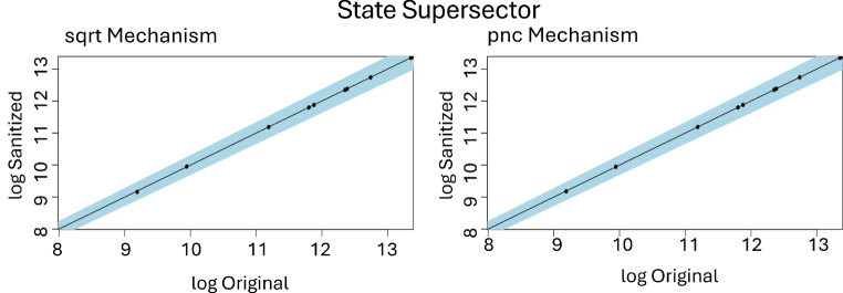
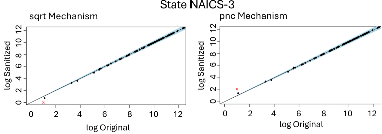
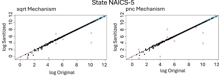
Figure 1. (Employment) Scatter plot of confidentiality-preserving microdata vs. ground truth for the groups in group-by queries for the workflow based on the $\sqrt{\phantom{x}}$-mechanism (first column) and pnc-mechanism (second column). The blue band shows $\pm 3\%$ of the original value. Points outside this band are colored red.Only the smallest groups (where error must be large to protect confidentiality) have values that are further than $3\%$ from the ground truth.

We next describe the settings for the experiment on QCEW data for which we have permission to share results, which only cover employment data (not wages).The measurement queries are the group-by queries for which the mechanisms produced noisy answers for the 3 monthly employment counts using the following groupings: (Q1) Identity – no grouping, (Q2) State total – grouping all establishments in the (redacted) state covered by the data, (Q3) 5-digit NAICS prefix, (Q4) County, (Q5) County by 5-digit NAICS prefix. For each of the 3 months, the respective query budgets were: (Q1) $0.7$, (Q2) $0.2$, (Q3) $0.6$, (Q4) $0.6$, (Q5) $0.7$. This results in an overall privacy budget (square root of the sum of squares) $\mu=\sqrt{0.7^{2}*3+0.2^{2}*3+0.6^{2}*3+0.6^{2}*3+0.7^{2}*3}\approx 2.28$. The distance parameter for employment was ${{\color[rgb]{0,0,0}\gamma}}_{emp}=0.5$. The pnc-mechanism confidence parameter was ${{\color[rgb]{0,0,0}\zeta}}=0.01$ (i.e., with probability $0.99$, no group-by query was changed by clipping). The noisy measurement query answers are postprocessed into confidentiality-preserving microdata. The evaluation queries are the group-by queries for which we evaluated accuracy – they can be different from the measurement queries.Table 3 shows the signed difference between employment group-by-queries computed from the confidentiality-preserving microdata and the ground truth (i.e., we don’t take the absolute value). Negative numbers indicate a negative difference (i.e., downward bias). In addition to state total, the groupings used for evaluation are supersector (2-digit NAICS prefix) and 5-digit NAICS prefix. The table summarizes the differences by computing the quartiles across groups in the group-by-queries (for state total, all establishments are grouped together into 1 group, so all quartiles are the same). We see that using the pnc-mechanism produces greater accuracy and less bias. This serves as additional empirical validation for Section 7, as it shows the pnc-mechanism reduces bias in the microdata. Some bias is still present because usage of the pnc-mechanism requires that the identity query be answered by the $\psi$-mechanism (with all other group-by queries answered by the pnc-mechanism).Figure 1 shows a scatter-plot of true vs. noisy answers for individual groups within employment group-by-queries (supersector, 3-digit NAICS prefix, 5-digit NAICS prefix), with a 3% band around the true value. Points outside the band are colored red. The results show both methods are accurate. All but the smallest groups have answers within $3\%$ of the true value. The groups with small employment counts, especially if they contain few establishments, would raise the most confidentiality concerns, and therefore should exhibit large errors. This is reflected by more red points in fine-grained groupings (e.g., group by 5-digit NAICS prefix) compared to coarser groupings (e.g., group by 3-digit NAICS prefix).

8.2. Evaluations on Synthetic Data

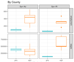
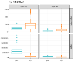
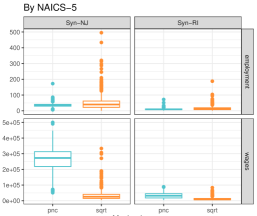
Figure 2. Absolute error averaged across 34 replications for employment group-by queries (top) and wages (bottom) for Synthetic New Jersey and Synthetic Rhode Island data.

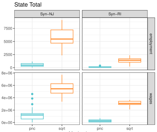
Figure 3. Absolute error of trivial grouping at state-level for employment (top) and wages (bottom) for Synthetic New Jersey and Synthetic Rhode Island data across 34 replicates.

Since experiments on confidential QCEW data are limited by policy, we synthesized a dataset with the same schema using public information (Bureau, 2024a, b; Eckert et al., 2020a) and statistical imputation (see the appendix for details). We use synthetic New Jersey (Syn-NJ) and Synthetic Rhode Island (Syn-RI) data, which serve as examples of fairly large and fairly small states, for further experimentation. This allows us to add results for wages as well. Synthetic New Jersey (Syn-NJ) includes 208,868 establishments and 21 counties.The number of establishments in a county ranges from 999 to 28,689 with mean 9,894, median 9,385 and standard deviation 6,968.The number of establishments for different NAICS codes present in Syn-NJ ranges from 1 to 8,172 with mean 364 and median 79 – so this distribution is highly skewed.Synthetic Rhode Island has only 5 counties and 25,420 establishments. The number of establishments in a county ranges from 1,102 to 14,414 with mean 5,084, median 3,354, and standard deviation 5,340. The number of establishments for different NAICS codes present in Syn-RI ranges from 1 to 610, with mean 13, median 4 and standard deviation 34.For the privacy settings, we set the privacy budget allocation for wages to be the same as the QCEW allocations for employment in Section 8.1 and then rescaled everything so that the total privacy budget was nearly the same as in Section 8.1. Specifically, each month of employment, and also the quarterly wages had the following privacy budgets for the group-by query groupings: (Q1) Identity – no grouping: 0.611, (Q2) State total – grouping all establishments in the same: 0.179, (Q3) 5-digit NAICS prefix: 0.525, (Q4) County: 0.525, (Q5) County by 5-digit NAICS prefix: 0.611. We used the distance parameter ${{\color[rgb]{0,0,0}\gamma}}_{w}=50$. The overall privacy budget was $\mu=\sqrt{0.611^{2}*4+0.179^{2}*4+0.525^{2}*4+0.525^{2}*4+0.611^{2}*4}\approx 2.31$.For each workflow (pnc-mechanism vs. $\sqrt{\phantom{x}}$-mechanism), we compute the absolute error of query answers and then repeat the experiment for 34 repetitions in order to assess variability of the errors.Figure 2 and 3 compare the absolute error achieved by pnc-mechanism and $\sqrt{\phantom{x}}$-mechanism for employment and wages on a variety of group-by queries on Synthetic New Jersey and Rhode Island. The figures summarize the errors using a box plot, which shows the median, upper and lower quartiles (the top and bottom of the box) and the spread of points outside the quartiles (the whiskers and dots outside the boxes). Figure 2 summarizes the absolute error for each group within a query is averaged across the replicates.The group-by queries cover (1) grouping by county to get county-level employment and wage totals, (2) grouping by 3-digit NAICS prefix – this is an important query that is not ameasurement query, and (3) grouping by 5-digit NAICS prefix – this is an important query and is expected to be sparse (i.e., many of the groups have very few establishments). Figure 3 summarizes the absolute error from each replicate of the trivial grouping in which all establishments are combined together to get state-level employment and wages totals.For employment counts (the top rows of the Figures 2 and 3 ), the pnc-mechanism performs substantially better than $\sqrt{\phantom{x}}$-mechanism. This is because the amount of noise injected into a group by $\sqrt{\phantom{x}}$-mechanism depends on the total within that group. However, the amount of noise added to a group by pnc-mechanism depends on the value of the largest establishment in the group. Specifically, ${\color[rgb]{0,0,0}pnc-mechanism}$ uses the noisy identity query to estimate simultaneous high-probability upper bounds on each establishment and then clips each establishment’s wages and employment to ensure that the upper bounds are not exceeded. It adds up the clipped values in a group, and then adds noise based on the largest establishment upper bound in the group. If no establishment dominates the group (i.e., is much larger than the rest), then the largest of the establishment upper bounds estimated by pnc-mechanism is significantly smaller than the total within a group, leading to less noise compared to $\sqrt{\phantom{x}}$-mechanism.Thus, for high-level aggregations like state total (Figure 3), there are so many establishments in a single group that no establishment can dominate the employment or wages. Hence pnc-mechanism significantly outperforms $\sqrt{\phantom{x}}$-mechanism on state totals. However, as the number of establishments in a group decreases, a single establishment is more likely to dominate the total within its group.For medium-level aggregations, like County (first plot of Figure 2), there is an increasing chance that some groups in the group-by queries contain a single establishment that can dominate the rest. Hence, the advantage of pnc-mechanism over $\sqrt{\phantom{x}}$-mechanism starts to decrease. It still performs better on employment and also Syn-RI wages, but the $\sqrt{\phantom{x}}$-mechanism is slightly better for Syn-NJ wages.The comparison for the NAICS-3 (second plot of Figure 2) and NAICS-5 (last plot of Figure 2) is particularly interesting because NAICS-5 is a sparse group-by query (this should benefit the $\sqrt{\phantom{x}}$-mechanism) containing many groups, and NAICS-3 is a non-measurement query (all the information about it contained in the confidentiality-preserving microdata mostly comes from the noisy answers to the group-by 5-digit NAICS prefix query). Surprisingly, we continue to see that pnc-mechanism outperforms $\sqrt{\phantom{x}}$-mechanism on employment counts for NAICS-5 and NAICS-3, although the difference between the performance of the two mechanisms has become very small.However, for total wages grouped by NAICS-3 or NAICS-5, we see that $\sqrt{\phantom{x}}$-mechanism clearly outperforms pnc-mechanism. This suggests that wages data are more highly skewed than employment count and an establishment is more likely to dominate the total wages in its industry than the total employment.The exact relationship between a group (in a group-by query) and which mechanism works best for it depends on the skewness in a group, the distance parameters, and privacy parameters. An interesting direction for future work is to use the confidentiality-preserving answers to the identity query to help estimate skewness in all groups of all group-by queries and (along with the public privacy parameters) to determine whether the pnc-mechanism or $\sqrt{\phantom{x}}$-mechanism should be used for a particular query.

9. Conclusions and Future Work

In this paper, we introduced Gaussian Establishment DP, a privacy definition for establishment data, designed to be interpretable to mathematical statisticians in statistical agencies. We proposed two mechanisms, the $\psi$-mechanism with non-releasable data-dependent variance, and the pnc-mechanism with releasable data-dependent variance. We showed that when converting noisy answers into microdata, one should avoid mechanisms with non-releasable variance whenever possible, because converting noisy query answers into microdata requires knowledge of how inaccurate the query answers could be (i.e., how much the answers can be trusted). Having to estimate the uncertainty therefore increases the error in the microdata and we showed that this can also introduce a downward bias.Future work includes predicting when one mechanism is more accurate than the other, based on the noisy answers to the identity query and privacy parameters. Another interesting direction is how to optimize a workload – adaptively selecting measurement queries and privacy budgets in order to maximize accuracy. Here again, the noisy identity query may be useful in estimating the expected gain in accuracy that can be obtained from candidate measurement queries.Acknowledgments: This work was supported by a NSF BAA grant. We thank Spencer Jobe for help with running our experiments on internal BLS data.

Appendix A Generation of Synthetic Evaluation data

We aim to create a synthetic establishment-level dataset that mirrors the structure of the QCEW data from publicly accessible data sources in order to run experiments to access our proposed privacy mechanisms and postprocessing procedures. The QCEW structure includes 18 variables, as described in Table 4.We use three main sources of publicly accessible data for this task: the Quarterly Workforce Indicators (QWI) (Bureau, 2024b), the County Business Patterns (CBP) dataset (Bureau, 2024a), and an employment count imputed CBP created by Eckert et al.(Eckert et al., 2020a, b). The variables of these datasets are summarized in Table 5. We focus on privately-owned establishment data from the 50 states for quarter 1 of 2016 since this matches the most recent imputed CBP dataset (Eckert et al., 2020a).There are four main steps to create the synthetic data. First, we combine the data sources by county and industry code. Next, we extract and impute monthly employment counts and quarterly wages for each county and NAICS-4 combination. Then, we get month 1 and 3 employment counts, quarterly wages, and number of establishments for each NAICS-6 by county combination. Finally, we generate establishment-level data that matches the QCEW structure.

Variable	Description
year	year of data; all entries $=2016$
qtr	quarter of data; all entries $=1$
state	SOC numeric state/territory value from 1 to 56
cnty	numeric county value, numbered within each state
naics	6-digit industry code using North American Industry ClassificationSystem (NAICS)
naics5, naics4, naics3	5, 4, and 3 digit industry code respectively
sector	2-digit NAICS sector code
supersector	BLS sector code groups NAICS sectors
own	ownership code (our data is all code-$5=$ “privately owned”)
m1emp, m2emp, m3emp	monthly employment counts
wage	total quarterly wages
primary_key	unique identifier for each establishment
can_agg	(metadata variable) all entries =”Y”
rectype	(metadata variable) all entries =”C”

Table 4. Variables for the establishment-level synthetic microdata.

A.1. Public Access Data

The U.S. Census offers many publicly accessible datasets that contain information similar to the QCEW data, namely the Quarterly Workforce Indicators (QWI) (Bureau, 2024b) and the County Business Patterns (CBP) (Bureau, 2024a). The CBP dataset has values aggregated at the County by NAICS-6 level up to the County by Sector level, while county by NAICS-4 is the most precise aggregation level of the QWI dataset. Additionally, both datasets have many missing and suppressed values (Table 6).The CBP dataset includes values for number of establishments (estnum), a mid-March (month 3 of quarter 1) employment count (emp) and quarterly total payroll values (qp1) (Table 5). The CBP dataset is not ideal for creating the monthly employment counts for the synthetic QCEW data, since it only has one of the three monthly employment counts that the QCEW data has. The QWI dataset has several employment variables discussed in Table 5: the employment at the beginning and end of the quarter (Emp and EmpEnd respectively) and the number of workers stably employed through the whole quarter (EmpS). The CBP data can help fill suppressed QWI month 3 employment values, especially since Eckert et al. have imputed the 2016 suppressed CBP employment values up to the county by NAICS-6 level and released the imputed dataset (Eckert et al., 2020a). The quarterly payroll value of the CBP data is a good base for the total quarterly data. However, 50% of qp1 are suppressed at the county by NAICS-4 level and the imputed CBP dataset does not include wages (Table 10. The QWI dataset has the average monthly earnings of workers employed at the beginning of the quarter (EarnBeg) and only 2% of the county by NAICS-4 cells are suppressed. Using EarnBeg and the monthly employment counts we can fill in suppressed values at the county by NAICS-4 level. For denoting a variable from here on, we refer to it by its data source, public attribute grouping, and then variable name. For example, QWI.cnty.EmpEnd is the employment at the end of the quarter at the county level from the QWI dataset.

All Datasets (never suppressed)
Public Attributes	state, county, sector, NAICS3, NAICS4
County Business Patterns (CBP) (Bureau, 2024a)
Public Attribute Levels	County by Sector (cntySect), County by NAICS-3 (cntyN3) to County by NAICS-6 (cntyN6)
Variables	estnum: the number of establishments
	qp1: quarterly total payroll values
Imputed CBP (imputeCBP) (Eckert et al., 2020a)
Public Attribute Levels	County by Sector (cntySect), County by NAICS-3 (cntyN3) to County by NAICS-6 (cntyN6)
Variable	emp: the imputed month 3 employment count
Quarterly Workforce Indicators (QWI) (Bureau, 2024b)
Public Attribute Levels	County (cnty), County by NAICS4 (cntyN4)
Variables	Emp: Beginning of quarter employment
	EmpEnd: End of quarter employment
	EmpS: number of employees who work the whole quarter
	EarnBeg: average month 1 earnings of workers

Table 5. The three public access datasets we use have a variety of variables describing the number of establishments, the number of employees, and the quarterly wages aggregated at various county and industry levels. Within the text, we refer to a variable by its data source, public attribute grouping, and then variable name. For example, CBP.cntyN4.qp1 is the quarterly total payroll aggregated by county and NAICS4 from the CBP dataset.

	Geographic Level
	cntySect	cntyN3	cntyN4	cntyN5	cntyN6
CBP.estnum	0 (0%)	0 (0%)	0 (0%)	0 (0%)	0 (0%)
CBP.qp1	10,813 (18%)	67,190 (36%)	210,047 (50%)	393,634 (58%)	480,987 (61%)
imputeCBP.emp	0 (0%)	0 (0%)	0 (0%)	0 (0%)	0 (0%)

	Geographic Level
	cnty	cntyN4
QWI.Emp	1 (0%)	187,814 (43%)
QWI.EmpEnd	1 (0%)	189,021 (43%)
QWI.EmpS	1 (0%)	184,082 (42%)
QWI.EarnBeg	0 (0%)	8,100 (2%)

Table 6. The number suppress values at each public attribute group level for each variable. The percent of rows at a given level that are suppressed in shown in parentheses.

A.2. Synthetic County by NAICS-4 Data

Since the the NAICS-4 by county level is the most specific level of public attribute groups in the QWI data, we start by creating a dataset of monthly employment counts and quarterly wages at this level. We describe the process in detail and in Algorithms 1 to 4. Algorithm 1 gets the monthly employment values and uses Algorithm 2 to get the month 2 employment count. Algorithm 2 is used in the final stage of the data generation as well to get the establishment level month 2 employment counts. Algorithm 3 is for the wage values and uses Algorithm 4 to bound the wages above using hierarchical industry values.We use a combination of QWI.cntyN4.Emp, QWI.cntyN4.EmpEnd, and imputeCBP.cntyN4.emp to generate the monthly employment counts for the county by NAICS-4 code cells (Algorithm 1). We denote these monthly employment counts as cntyN4.m1emp, cntyN4.m2emp, and cntyN4.m3emp to avoid confusion with the monthly employment counts at the establishment level or at the county by NAICS-6 level.When QWI.cntyn4.Emp values are not suppressed, we set cntyn4.m1emp to be equal to them. However, when they are suppressed we use a regression model to impute the values.First, we fit the model on the rows where QWI.cntyN4.Emp and QWI.cntyN4.EmpEnd are available. The following linear model is used:

(2) $$\texttt{QWI.cntyN4.Emp}_{c,k}=\beta_{0}+\beta_{1}\texttt{QWI.cntyN4.EmpEnd}_{c,k}+\beta_{2}\texttt{CBP.cntyN4.estnum}_{c,k}+\beta_{3}\texttt{cntyN4.state}_{c,k}+\beta_{4}\texttt{cntyN4.sector}_{c,k}+\epsilon_{c,k}$$

where $\epsilon_{c,k}\overset{iid}{\sim}N(0,\sigma^{2})$ for all $(c,k)$ such that $\texttt{QWI.cntyN4.Emp}_{c,k}$ and $\texttt{QWI.cntyN4.EmpEnd}_{c,k}$ are not missing for the combination of county code $c$ and NAICS-4 code $k$. This model was selected to include both geographic and industry code features as well as the number of establishments in cell. For the geographic predictor variable, we cannot use county as a predictor since there are counties that suppress all QWI.cntyN4.Emp values. State is used as the geographic predictor instead. Sector is used for similar reasons. Once the model is fitted, we check that the residuals for normality and equal variance, and identify one outlier. The model is refitted without the outlier. If QWI.cntyN4.EmpEnd is suppressed, we use the impute.cntyN4.emp as the predictor. Then we simulate the missing cntyN4.m1emp values using the refitted model. The QWI.cntyN4.EmpEnd filled with the imputeCBP.cntyN4.emp values are used as month 3 employment counts.Then we generate month 2 employment counts using Algorithm 2 and noise parameter $\eta=1.69$. This algorithm sets cntyN4.m2emp to zero if month 1 and 3 employment counts are zero. Otherwise the change from the midpoint of month 1 and 3 is randomly generated from a normal distribution with mean $0$ and variance proportional to the ratio of the absolute difference and the average of the monthly employment values. More specifically, the variance is $\sigma^{2}=\eta\frac{|\texttt{cntyN4.m3emp}-\texttt{cntyN4.m1emp}|}{\texttt{cntyN4.m1emp}+\texttt{cntyN4.m3emp}}$. Thus there is more variation from the midpoint when the monthly employment counts are vastly different. When the change between month 1 and month 3 is large relative to the monthly employment counts, the variation from the midpoint will be larger than if the same change is small relative to the monthly employment counts. If industries with a large number of employees are likely to have more steady changes in employment than small but fast-growing industries, then this algorithm mimics that behavior. The Month 2 Employment Algorithm is also used later when generating the establishment level month 2 employment counts.

Input: QWI.cntyN4.Emp, QWI.cntyN4.EmpEnd, QWI.cntyN4.EmpS;

/* county by NAICS-4 employment values from QWI */

1

QWI.cnty.Emp ;

/* county-level employment values from QWI */

2

imputeCBP.cntyN4.emp, CBP.cntyN4.estnum ;

/* county by NAICS-4 values from CBP and imputed CBP */

3

$\mathcal{I}=\{(c,k):(c,k)\in\texttt{QWI.cntyN4}\cap\texttt{imputeCBP.cntyN4}\}$, ;

/* county by NAICS-4 indices in QWI and imputed CBP */

4

cntyN4.state, cntyN4.sector, ;

/* state and sector corresponding to county by NAICS-4 cells */

5

$\eta>0$ ;

/* noise parameter for m2emp */

6

/* Defining sets of indices based on missing values */

7Let $\mathcal{I}_{/\texttt{Emp}}=\{(c,k)\in\mathcal{I}:\texttt{QWI.cntyN4.Emp}_{c,k}\text{ is missing}\}$;

8Let $\mathcal{I}_{/\texttt{EmpEnd}}=\{(c,k)\in\mathcal{I}:\texttt{QWI.cntyN4.EmpEnd}_{c,k}\text{ is missing}\}$;

9Let $\mathcal{I}_{*}=\{(c,k)\in\mathcal{I}:\texttt{QWI.cntyN4.Emp}_{c,k}\text{ and }\texttt{QWI.cntyN4.EmpEnd}_{c,k}\text{ are not missing}\}$;

/* Fit a model to predict QWI.cntyN4.Emp from QWI.cntyN4.EmpEnd and other predictors. */

10Fit model (2) with $(c,k)\in\mathcal{I}_{*}$;

11If necessary, identify outliers based on residual normality plot and fitted verses residual plot. Remove them and refit model (2);

12Let $\hat{f}_{\texttt{cntyN4.Emp}}(\cdot)$ be the function that takes in the predictor variable values and returns the fitted value of the model;

13Let $se_{pred}(\hat{y})$ be the function that takes in a fitted value, $\hat{y}$, from the model and returns the standard error of the prediction;

14foreach $(c,k)\in\mathcal{I}_{*}$ do

   $\texttt{m3emp}_{c,k}\leftarrow\texttt{QWI.cntyN4.EmpEnd}_{c,k}$;

    /* use QWI.cntyN4.Emp and QWI.cntyN4.EmpEnd is available */

15   $\texttt{m1emp}_{c,k}\leftarrow\texttt{QWI.cntyN4.Emp}_{c,k}$

16foreach $(c,k)\in\mathcal{I}_{/\texttt{EmpEnd}}$ do

   $\texttt{m3emp}_{c,k}\leftarrow\texttt{imputeCBP.cntyN4.emp}_{c,k}$ ;

    /* use imputeCBP.cntyN4.emp if QWI.cntyN4.EmpEnd is missing */

17   

18foreach $(c,k)\in\mathcal{I}_{/\texttt{Emp}}$ do

19   $\hat{y}_{c,k}\leftarrow\hat{f}_{\texttt{cntyN4.Emp}}(\texttt{m3emp}_{c,k},\texttt{CBP.cntyN4.estnum},\texttt{QWI.cntyN4.state},\texttt{QWI.cntyN4.sector})$;

   $\texttt{m1emp}_{c,k}\leftarrow\hat{y}_{c,k}+Z_{c,k}$ where $Z_{c,k}\overset{indep.}{\sim}N(0,se_{pred}^{2}(\hat{y}_{c,k}))$;

    /* use refitted model if QWI.cntyN4.Emp is missing */

20   

21foreach $(c,k)\in\mathcal{I}$ do

22   $\texttt{m2emp}_{c,k}\leftarrow\text{Month 2 Employment}(\eta,\texttt{m1emp}_{c,k},\texttt{m3emp}_{c,k})$ where Month 2 Employment is Algorithm 2if $\texttt{QWI.cntyN4.EmpS}_{c,k}$ is not missing then

      $\texttt{m}M\texttt{emp}_{c,k}=\max(\texttt{m}M\texttt{emp}_{c,k},\texttt{QWI.cntyN4.EmpS}_{c,k})$ for $M=1,2,3$ ;

       /* QWI.cntyN4.EmpS lower bound if available */

23      

24   else

      $\texttt{m}M\texttt{emp}_{c,k}=\max(\texttt{m}M\texttt{emp}_{c,k},0)$ for $M=1,2,3$ ;

       /* lower bound by 0 if QWI.cntyN4.EmpS is missing */

25      

26   

/* Adjust m1emp values from model using the county total value QWI.cnty.Emp if available. */

27foreach $c^{\prime}$ such that $(c^{\prime},k)\in\mathcal{I}_{/\texttt{Emp}}$ do

28   if $\texttt{QWI.cnty.Emp}_{c^{\prime}}$ is not missing then

29      Let $\mathcal{I}_{c^{\prime},model}=\{k:(c^{\prime},k)\in\mathcal{I}_{/\texttt{Emp}}\}$;

30      $\Sigma_{c^{\prime},model}\texttt{m1emp}\leftarrow\sum_{k\in\mathcal{I}_{c^{\prime},model}}\texttt{m1emp}_{c^{\prime},k}$;

31      $\Sigma_{c^{\prime},QWI}\texttt{QWI.cntyN4.Emp}\leftarrow\sum_{k\in\mathcal{I}_{c^{\prime},QWI}}\texttt{QWI.cntyN4.Emp}_{c^{\prime},k}$ where $\mathcal{I}_{c^{\prime},QWI}=\{k:(c^{\prime},k)\in\mathcal{I}^{C}_{/\texttt{Emp}}\}$;

32      if $\Sigma_{c^{\prime},model}\texttt{m1emp}\neq 0$ then

33         $\texttt{m1emp}_{c^{\prime},k}\leftarrow\texttt{m1emp}_{c^{\prime},k}+(\texttt{QWI.cnty.Emp}_{c^{\prime}}-\Sigma_{c^{\prime},QWI}\texttt{QWI.cntyN4.Emp})\frac{\texttt{m1emp}_{c^{\prime},k}}{\Sigma_{c^{\prime},model}\texttt{m1emp}}$ for each $k\in\mathcal{I}_{c^{\prime},model}$

34      else

35         $\texttt{m1emp}_{c^{\prime},k}\leftarrow\texttt{m1emp}_{c^{\prime},k}+\frac{1}{|\mathcal{I}_{c^{\prime},model}\texttt{m1emp}|}(\texttt{QWI.cnty.Emp}_{c^{\prime}}-\Sigma_{c^{\prime},QWI}\texttt{QWI.cntyN4.Emp})$ for each $k\in\mathcal{I}_{c^{\prime},model}$

36      

37   

38Let cntyN4.m1emp be a vector of $\max(0,\texttt{m1emp}_{c,k})$ for $(c,k)\in\mathcal{I}$;

39Let cntyN4.m2emp be a vector of $\max(0,\texttt{m2emp}_{c,k})$ for $(c,k)\in\mathcal{I}$;

40Let cntyN4.m3emp be a vector of $\max(0,\texttt{m3emp}_{c,k})$ for $(c,k)\in\mathcal{I}$;

Result: $\texttt{cntyN4.m1emp},\texttt{cntyN4.m2emp},\texttt{cntyN4.m3emp}$

Algorithm 1 (Employment for County by NAICS-4) We use QWI.cntyN4.Emp and QWI.cntyN4.EmpEnd as m1emp and m3emp when available. Otherwise, we use impute.CBP.cntyN4.emp as m3emp and predict m1emp from a model fitted on a combination of QWI.cntyN4 and CBP.cntyN4 variables. Then m2emp is derived from Algorithm 2. Adjustments to the employment counts are made based on QWI.cnty.Emp and QWI.cntyN4.EmpS when available. For an set of indices such as $\mathcal{I}_{*}$ let the complement be denoted $\mathcal{I}^{C}_{*}$. Let the sum of values over an empty set be equal to $0$.

Now that all three monthly employment counts have been determined, we check and adjust these values. First, if a stable employment count QWI.cntyN4.EmpS is available, we force this value to be a lower bound on each monthly employment count. We then use in county total QWI.cnty.Emp values to adjust any model-simulated m1emp values. Denote the value for county $c$ as $\texttt{QWI.cnty.Emp}_{c}$. We are unable to adjust the values in Kalawao County, Hawaii (FIPS code 15005), since the county total is suppressed. For each other county, we sum the QWI.cntyN4.Emp values in the county and sum the m1emp values that came from the fitted model for that county. For county $c$, denote the sum of the QWI.cntyN4.Emp data as $\Sigma_{c,QWI}\texttt{Emp}$ and the sum from the fitted model as $\Sigma_{c,model}\texttt{m1emp}$. If $\Sigma_{c,model}\texttt{m1emp}\neq 0$, then each model-fitted m1emp is adjusted proportional to its share of the model-fitted sum:

$$\texttt{cntyN4.m1emp}_{c,k}=\texttt{cntyN4.m1emp}_{c,k}+\left(\texttt{QWI.cnty.Emp}_{c}-\Sigma_{c,QWI}\texttt{QWI.cntyN4.Emp}\right)\frac{\texttt{cntyN4.m1emp}}{\Sigma_{c,model}\texttt{m1emp}}.$$

Otherwise m1emp is adjusted by $(\texttt{QWI.cnty.Emp}_{c}-\Sigma_{c,QWI}\texttt{QWI.cntyN4.Emp})$ over the number of cells that were simulated from the model.

Input: $\eta>0$, m1emp$\geq 0$, and m3emp$\geq 0$

1if $\texttt{m1emp}=\texttt{m3emp}=0$ then

2   $\texttt{m2emp}=0$

3else

4   $\sigma^{2}=2\eta\frac{|\texttt{m3emp}-\texttt{m1emp}|}{\texttt{m3emp}+\texttt{m1emp}}$;

5   Generate $Z\sim\operatorname{Normal}(0,\sigma^{2})$;

6   $\texttt{m2emp}=\texttt{m1emp}+\frac{\texttt{m3emp}-\texttt{m1emp}}{2}+Z$;

7   if $\texttt{m2emp}\leq 0$ then

8      if $\texttt{m3emp}=0|\texttt{m1emp}=0$ then

9         $\texttt{m2emp}=0$

10      else

11         $\texttt{m2emp}=1$

12      

13   

Result: m2emp

Algorithm 2 (Month 2 Employment) Using a noise parameter $\eta$, we make a m2emp value from the m1emp and m3emp values. This algorithm is used within Algorithms 1 and 7

Finally, we can consider the wage values using Algorithm 3. If the CBP.cntyN4.qp1 value is not suppressed, it is used as the wage value. Otherwise, if the average monthly employee earnings at the beginning of the quarter QWI.cntyN4.EarnBeg is available,then we set $\texttt{wage}=\texttt{QWI.cntyN4.EarnBeg}(\texttt{cntyN4.m1emp}+\texttt{cntyN4.m2emp}+\texttt{cntyN4.m3emp})$ where the monthly employment counts are from Algorithm 1. For the remaining missing NAICS-4 by county cells, we use a regression model. Instead of predicting the wage value outright, we predict the difference between the county by NAICS-4 wage value and the sum of available county by NAICS-6 wage value within the NAICS-4 code.First, we get the sum of the available NAICS-6 CBP.cntyN6.qp1 values and the count of suppressed NAICS-6 cells corresponding to the NAICS-4 by county cell. For NAICS-4 code $k$ and county $c$, denote the sum of available NAICS-6 values as $\Sigma^{(6,4)}_{c,k}$, the count of suppressed cells as $M_{c,k}$. If there are no available county by NAICS-6 values for county $c$ and NAICS-4 code $k$, then $\Sigma^{(6,4)}_{c,k}=0$. For cells that have a CBP.cntyN4.qp1 value available, we fit a model:

$$\sqrt{\texttt{CBP.cntyN4.qp1}_{c,k}-\Sigma^{(6,4)}_{c,k}} =\beta_{0}+\beta_{1}\texttt{cntyN4.state}_{c,k}+\beta_{2}\texttt{cntyN4.sector}_{c,k}+\beta_{3}M_{c,k}+\beta_{4}\texttt{cntyN4.m3emp}_{c,k}$$

(3) $$\phantom{=}+\beta_{5}\texttt{cntyN4.m3emp}_{c,k}M_{c,k}+\beta_{6}\texttt{cntyN4.m3emp}_{c,k}^{2}+\beta_{7}\texttt{cntyN4.m3emp}_{c,k}^{3}+\epsilon_{c,k}$$

where $\epsilon_{c,k}\overset{iid}{\sim}\operatorname{Normal}(0,\sigma^{2})$. The predictors cntyN4.state and cntyN4.sector were chosen for similar reasons as the model in (2). The number of suppressed cells is important when predicting the amount missing from a cell higher in the hierarchy of industry codes. The cntyN4.m3emp is chosen over the other monthly employment counts since it was not imputed by our model (2). The square root transformation of the response variable is select trial and error until the residual plots suggested the assumptions on the residuals seemed reasonable. The structure of the equation for the predictors was chosen based on trial and error and comparing the AIC and residual plots across considered models.Once the model is fitted, we find five outliers (FIPS_NAICS-4: 21033_4452, 21107_5619, 36007_2361, 6007_3399, 6109_5231). These are removed and the model is refitted. For the wage cells at the NAICS-4 by county level that are not generate from CBP.cntyN4.qp1 or QWI.cntyN4.EarnBeg, we simulate $\sqrt{\texttt{qp1}_{c,k}-\Sigma_{c,k}^{(6,4)}}$ using the refitted model. Since $\Sigma^{(6,4)}_{c,k}$ is known for all combinations of counties and NAICS-4 codes, we transform the simulated value from the model to generate $\texttt{wage}_{c,k}$ which becomes the wage value for county $c$ and NAICS-4 code $k$. Then we bound all $\texttt{wage}_{c,k}$ values below by $\Sigma_{c,k}^{(6,4)}$. In Algorithm 4, we find an upper bound for $\texttt{wage}_{c,k}$ using information from the county by NAICS-3, and county by NAICS sector and county levels. Denote the sum of available $d$-digit NAICS qp1 values in the code $k$ of NAICS $r$ level for county $c$ as $\Sigma_{k,c}^{(d,r)}$. If the NAICS-3 by county $\texttt{CBP.cntyN3.qp1}_{c,j}$ value is not suppressed where $j$ is the NAICS-3 code corresponding to NAICS-4 code $k$, then the maximum $\texttt{wage}_{c,k}$ is $\texttt{CBP.cntyN3.qp1}_{c,j}-\Sigma_{c,k}^{(4,3)}$. Otherwise, if the NAICS sector (i.e. 2 digit NAICS) by county $\texttt{CBP.cntySect.qp1}_{c,i}$ value is not suppressed where $i$ is the NAICS Sector corresponding to NAICS-4 code $k$, then the maximum is $\texttt{CBP.cntySect.qp1}_{c,i}-\Sigma_{c,k}^{(3,2)}$. If both the NAICS 3-digit and NAICS sector are suppressed, we use the county total wages minus the sum of available NAICS sector wages as the maximum.

Input: QWI.cntyN4.EarnBeg, ;

/* county by NAICS-4 average earnings values from QWI */

1

cntyN4.m1emp,cntyN4.m2emp, cntyN4.m3emp ;

/* county by NAICS-4 employment values from Algorithm 1 */

2

CBP.cntyN6.qp1,CBP.cntyN4.qp1, CBP.cntyN3.qp1,CBP.cntySect.qp1, CBP.cnty.qp1 ;

/* quarterly payroll values */

3

$\mathcal{I}=\{(c,k):(c,k)\in\texttt{QWI.cntyN4}\cap\texttt{CBP.cntyN4}\}$, ;

/* county by NAICS-4 indices in QWI and CBP */

4

cntyN4.state, cntyN4.sector, ;

/* state and sector corresponding to county by NAICS-4 cells */

5

6foreach $(c,k)\in\mathcal{I}$ do

7   Let $\mathcal{I}_{c,k}^{(6,4)}=\{\ell\in\text{NAICS-6 codes within }k:\texttt{CBP.cntyN6.qp1}_{c,\ell}\text{ is not missing}\}$;

8   $\Sigma_{c,k}^{(6,4)}\leftarrow\sum_{\ell\in\mathcal{I}_{c,k}^{(6,4)}}\texttt{CBP.cntyN6.qp1}_{c,\ell}$$M_{c,k}\leftarrow|\{\ell\in\text{NAICS-6 codes within }k:\texttt{CBP.cntyN6.qp1}_{c,\ell}\text{ is suppressed}\}|$;

9Let $\mathcal{I}_{/\texttt{cntyN4.qp1}}=\{(c,k)\in\mathcal{I}:\texttt{CBP.cntyN4.qp1}\text{ is missing}\}$ ;

10Let $\mathcal{I}_{/\texttt{EarnBeg}}=\{(c,k)\in\mathcal{I}:\texttt{QWI.cntyN4.EarnBeg}\text{ is missing}\}$;

11foreach $(c,k)\in\mathcal{I}^{C}_{/\texttt{cntyN4.qp1}}$ do

   $\texttt{wage}_{c,k}\leftarrow\texttt{CBP.cntyN4.qp1}_{c,k}$ ;

    /* use CBP.cntyN4.qp1 if available */

12   

13Fit model (A.2) with $(c,k)\in\mathcal{I}^{C}_{/\texttt{cntyN4.qp1}}$;

14If necessary, identify outliers based on residual normality plot and fitted verses residual plot. Remove them and refit model (A.2);

15Let $\hat{f}_{\texttt{cntyN4.qp1}}(\cdot)$ be the function that takes in the predictor variable values and returns the fitted value of the model;

16Let $se_{pred}(\hat{y})$ be the function that takes in a fitted value, $\hat{y}$, from the model and returns the standard error of the prediction;

17foreach $(c,k)\in\mathcal{I}_{/\texttt{cntyN4.qp1}}\cap\mathcal{I}_{/\texttt{EarnBeg}}$ do

18   $\hat{y}_{c,k}\leftarrow\hat{f}_{\texttt{cntyN4.qp1}}(\texttt{cntyN4.state},\texttt{cntyN4.sector},M_{c,k},\texttt{cntyN4.m3emp})$;

   $\texttt{wage}_{c,k}\leftarrow(\hat{y}_{c,k}+Z_{c,k})^{2}+\Sigma_{c,k}^{(6,4)}$ where $Z_{c,k}\overset{indep.}{\sim}N(0,se_{pred}^{2}(\hat{y}_{c,k}))$ ;

    /* predict wage value with model */

19   

20foreach $(c,k)\in\mathcal{I}_{/\texttt{cntyN4.qp1}}\cap\mathcal{I}^{C}_{/\texttt{EarnBeg}}$ do

21   $w\leftarrow\texttt{QWI.cntyN4.EarnBeg}_{c,k}(\texttt{cntyN4.m1emp}_{c,k}+\texttt{cntyN4.m2emp}_{c,k}+\texttt{cntyN4.m3emp}_{c,k})$;

   $\texttt{wage}_{c,k}\leftarrow\max(w,\Sigma_{k,c}^{(6,4)})$ ;

    /* lower bound is $\Sigma_{k,c}^{(6,4)}$ */

22   

/* Adjust based on an upper bound for the wage value */

23foreach $(c,k)\in\mathcal{I}_{/\texttt{cntyN4.qp1}}$ do

24   $u_{c,k}\leftarrow\text{Wage Upper Bound}(c,k,\texttt{CBP.cntyN3.qp1},\texttt{CBP.cntySct.qp1},\texttt{CBP.cnty.qp1})$ where Wage Upper Bound is Algorithm 4;

25   $\texttt{wage}_{c,k}=\min(u_{c,k},\texttt{wage}_{c,k})$

26cntyN4.wage is a vector of $\texttt{wage}_{c,k}$ for $(c,k)\in\mathcal{I}$;

Result: cntyN4.wage

Algorithm 3 (Wage for County by NAICS-4) For an set of indices such as $\mathcal{I}_{/\texttt{cntyN4.qp1}}$ let the complement be denoted $\mathcal{I}^{C}_{/\texttt{cntyN4.qp1}}$.Let any sum of values over an empty set be equal to $0$.

Input: $(c,k)$;

/* county and NAICS-4 code */

1

CBP.cntyN3.qp1,CBP.cntySect.qp1, CBP.cnty.qp1;

/* quarterly payroll values from CBP data */

2

3$i$ and $j$ are the Sector and the NAICS-3 codes corresponding to NAICS-4 code $k$, respectively;

4if $\texttt{CBP.cntySect.qp1}_{c,i}$ is not missing then

5   Let $\mathcal{I}_{c,k}^{(3,2)}=\{j^{\prime}\in\text{NAICS-3 codes within Sector code }i:\texttt{CBP.cntyN3.qp1}_{c,j^{\prime}}\text{ is not missing}\}$;

6   $u_{c,k}\leftarrow\texttt{CBP.cntySect.qp1}_{c,i}-\sum_{j^{\prime}\in\mathcal{I}_{c,k}^{(3,2)}}\texttt{CBP.cntyN3.qp1}_{c,j^{\prime}}$

7if $\texttt{CBP.cntyN3.qp1}_{c,j}$ is not missing then

8   Let $\mathcal{I}_{c,k}^{(4,3)}=\{k^{\prime}\in\text{NAICS-4 codes within NAICS-3 code }j:\texttt{CBP.cntyN4.qp1}_{c,k^{\prime}}\text{ is not missing}\}$;

9   $u_{c,k}\leftarrow\texttt{CBP.cntyN3.qp1}_{c,j}-\sum_{k^{\prime}\in\mathcal{I}_{c,k}^{(4,3)}}\texttt{CBP.cntyN4.qp1}_{c,k^{\prime}}$

10if $\texttt{CBP.cntyN3.qp1}_{c,j}$ and $\texttt{CBP.cntySect.qp1}_{c,i}$ are missing then

11   Let $\mathcal{I}_{c,k}^{(2)}=\{i^{\prime}\in\text{NAICS Sectors codes that appear in county }c:\texttt{CBP.cntySect.qp1}_{c,i^{\prime}}\text{ is not missing}\}$;

12   $u_{c,k}\leftarrow\texttt{CBP.cnty.qp1}_{c}-\sum_{i^{\prime}\in\mathcal{I}_{c,k}^{(2)}}\texttt{CBP.cntySect.qp1}_{c,j^{\prime}}$

Result: $u_{k,c}$

Algorithm 4 (Wage Upper Bound) Using the CBP data, we get an upper bound on the quarterly wages for county $c$ and NAICS-4 code $k$. Let the sum of qp1 values over an empty set be set equal to $0$.

A.3. Synthetic County by NAICS-6 Data

We use the NAICS-4 by county data to create a NAICS-6 by county dataset (Algorithm 5). First we identify any NAICS-4 and county combinations which only have one NAICS-6 code within them according the CBP data. For these cells we set cntyN6.m1emp, cntyN6.m3emp, and cntyN6.wage to be the values from the corresponding NAICS-4 level and add a column for the number of establishments CBP.cntyN6.estnum. Then we focus on the NAICS-6 by county cells that have not been filled by the NAICS-4 by county values.Since we are going to use the CBP imputed imputeCBP.cntyN6.emp value for the cntyN6.m3emp value at the NAICS-6 by county level, we need to adjust our imputeCBP.cntyN6.emp values to match the scale of the QWI.cntyN4.EmpEnd values from the QWI that inform some of the NAICS-4 cntyN4.m3emp values. We create a column in the NAICS-4 by county data,

$$\texttt{EmpScale}=\begin{cases}\frac{\texttt{imputeCBP.cntyN4.emp}}{\texttt{cntyN4.m3emp}}&\text{ if }\texttt{cntyN4.m3emp}>0\\ 1&\text{otherwise}\end{cases}.$$

For the NAICS-6 codes that did not automatically inherit the NAICS-4 value, we set cntyN6.m3emp to be the NAICS-6 imputeCBP.cntyN6.emp from the imputed CBP over the EmpScale for the corresponding county by NAICS-4 code. For example, in some county, consider the NAICS-4 code 2361, if the CBP imputeCBP.cntyN4.emp for NAICS-4 2361 is $1000$ and the QWI $\texttt{QWI.cntyN4.EmpEnd}=1250$, let our $\texttt{cntyN4.m3emp}=1250$ for that county and NAICS-4 combination. Then the $\texttt{EmpScale}=0.8$. If the county has CBP imputed $\texttt{imputeCBP.cntyN6.emp}=700$ for NAICS-6 code 236115 and $\texttt{imputeCBP.cntyN6.emp}=300$ for NAICS-6 code 236116, then our adjusted cntyN6.m3emp for that county are $875$ for NAICS 236115 and $375$ for NAICS 236116.

Input: cntyN4.m1emp, cntyN4.m2emp, cntyN4.m3emp, cntyN4.wage, ;

/* from Algorithms 1 and 3 */

1

CBP.cntyN6.qp1,CBP.cntyN6.estnum,imputeCBP.cntyN6.emp ;

/* county by NAICS-6 values */

2$\mathcal{I}_{\texttt{cntyN6}}=\{(c,k,\ell):\text{county, NAICS-4, and NAICS-6 code combination corresponding to }\texttt{imputeCBP.cntyN6}\text{ rows}\}$,

3$\mathcal{I}_{\texttt{cntyN4}}=\{(c,k):\text{county, NAICS-4 code combination corresponding to }\texttt{cntyN4.m3emp}\text{ rows}\}$

4foreach $(c,k)\in\mathcal{I}_{\texttt{cntyN4}}$ do

5   $\mathcal{I}_{c,k}=\{\ell:(c,k,\ell)\in\mathcal{I}_{\texttt{cntyN6}}\}$;

6   if $|\mathcal{I}_{c,k}|=1$ then

7      $\texttt{m1emp}_{c,\ell}=\texttt{cntyN4.m1emp}_{c,k}$ for $\ell\in\mathcal{I}_{c,k}$;

8      $\texttt{m3emp}_{c,\ell}=\texttt{cntyN4.m3emp}_{c,k}$ for $\ell\in\mathcal{I}_{c,k}$;

9      $\texttt{wage}_{c,\ell}=\texttt{cntyN4.wage}_{c,k}$ for $\ell\in\mathcal{I}_{c,k}$

10   else

11      if $\texttt{cntyN4.m3emp}_{c,k}>0$ and $\texttt{imputeCBP.cntyN4.emp}_{c,k}>0$ then

12         $\texttt{EmpScale}_{c,k}=\frac{\texttt{imputeCBP.cntyN4.emp}_{c,k}}{\texttt{cntyN4.m3emp}_{c,k}}$;

13         $\texttt{m3emp}_{c,\ell}=\texttt{imputeCBP.cntyN6.emp}_{c,\ell}/\texttt{EmpScale}_{c,k}$ for all $\ell\in\mathcal{I}_{c,k}$

14      else

15         $\texttt{m3emp}_{c,k}=\texttt{imputeCBP.cntyN6.emp}_{c,\ell}$ for all $\ell\in\mathcal{I}_{c,k}$

16      $(\texttt{m1emp}_{c,\ell}:\ell\in\mathcal{I}_{c,k})^{T}\leftarrow\text{Dirichlet Divider}((\texttt{m3emp}_{c,\ell}:\ell\in\mathcal{I}_{c,k})^{T},\texttt{cntyN4.m1emp})$ where Dirichlet Divider is Algorithm 6;

17      $\mathcal{I}_{c,k}^{(6,4)}=\{\ell\in\mathcal{I}_{c,k}:\texttt{CBP.cntyN6.qp1}_{c,\ell}\text{ is not missing}\}$;

18      $\Sigma_{c,k}^{(6,4)}=\sum_{\ell\in\mathcal{I}_{c,k}^{(6,4)}}\texttt{CBP.cntyN6.qp1}_{c,\ell}$;

      $\texttt{wage}_{c,\ell}=\texttt{CBP.cntyN6.qp1}_{c,\ell}$ for $\ell\in\mathcal{I}_{c,k}^{(6,4)}$ ;

       /* use CBP.cntyN6.qp1 if available */

19      $A_{c,k}=\texttt{cntyN4.wage}_{c,k}-\Sigma_{c,k}^{(6,4)}$;

20      $(\texttt{wage}_{c,\ell}:\ell\in\mathcal{I}_{c,k}\cap\ell\notin\mathcal{I}_{c,k})^{T}\leftarrow\text{Dirichlet Divider}((\texttt{m3emp}_{c,\ell}:\ell\in\mathcal{I}_{c,k}\cap\ell\notin\mathcal{I}_{c,k})^{T},A_{c,k})$

21   

22cntyN6.wage is a vector of $\texttt{wage}_{c,\ell}$ for $(c,\ell)\in\mathcal{I}_{\texttt{cntyN6}}$;

23cntyN6.m1emp is a vector of $\texttt{m1emp}_{c,\ell}$ for $(c,\ell)\in\mathcal{I}_{\texttt{cntyN6}}$;

24cntyN6.m3emp is a vector of $\texttt{m3emp}_{c,\ell}$ for $(c,\ell)\in\mathcal{I}_{\texttt{cntyN6}}$;

25$\texttt{cntyN6.estnum}\leftarrow\texttt{CBP.cntyN6.estnum}$;

Result: cntyN6.m1emp, cntyN6.m3emp, cntyN6.wage, cntyN6.estnum

Algorithm 5 (County by NAICS-6)

To get a cntyN6.m1emp for each NAICS-6 by county we use an algorithm based on the Dirichlet distribution which we call the Dirichlet Divider (Algorithm 6). The algorithm uses a concentration vector parameter of size $d$ where $d$ is the desired output size. The algorithm randomly divides an inputted total value into $d$ subtotals proportional to the concentration parameter. In this case, our concentration parameter is cntyN6.m3emp at the NAICS-6 level corresponding to a given NAICS-4 code. If all concentration vector elements are $0$, the algorithm sets them all to be $1$. The algorithm generates an observation from a Dirichlet distribution that is a random vector of $d$ proportions that sum to 1. A inputted total value is multiplied by the random vector to get $d$ non-negative subtotals which sum to to the total. In this case we use the cntyN4.m1emp value from the corresponding NAICS-4 code as the total and the resulting subtotals become the cntyN6.m1emp values for the NAICS-6 by county codes. We will not get m2emp values again until we are at the establishment level.

Input: $\mathbf{b}=(b_{1}~b_{2}~\dots~b_{d})^{T}\in\mathbb{R}^{d}$ such that $b_{i}\geq 0$, total value $A\geq 0$

1if $b_{1}=b_{2}=\dots b_{d}=0$ then

2   $\mathbf{b}\leftarrow\mathbf{1}\in\mathbb{R}^{d}$

3Generate $\mathbf{p}\sim\operatorname{Dirichlet}(\mathbf{b})$ ;

4$(a_{1}~a_{2}~\dots~a_{d})^{T}\leftarrow\mathbf{p}A$;

Result: $\mathbf{a}=(a_{1}~a_{2}~\dots~a_{d})^{T}$

Algorithm 6 (Dirichlet Divider) Using a concentration input vector $\mathbf{b}\in\mathbb{R}^{d}_{\geq 0}$, the Dirichlet Divider randomly splits a total value $A$ into $d$ values, $a_{1},a_{2},\dots,a_{d}$ such that $A=\sum_{i=1}^{d}a_{i}$ and $a_{i}\geq 0$ for $i=1,\dots,d$.

Finally, we just need to derive wage values at the NAICS-6 by county level. We get the sum of NAICS-6-level CBP.cntyN6.qp1 for a specific NAICS-4 code, $\Sigma_{c,k}^{(6,4)}$. Then we get the difference between that sum and the cntyN4.wage value at the NAICS-4 level. For NAICS-6 codes within the specified NAICS-4 code that do not have CBP.cntyN6.qp1 values we use the Dirichlet Divider with the cntyN6.m3emp values as the concentration vector elements and $\texttt{CBP.cntyN4.qp1}_{c,k}-\Sigma_{c,k}^{(6,4)}$ as the total.

A.4. Establishment-level Synthetic Data

The last stage uses the County by NAICS-6 cell values and the Dirichlet Divider Algorithm 6 from previous steps (Algorithm 7). We randomly generate the concentration parameters for the Dirichlet Divider as independent and identically distributed random variables from a Gamma distribution with a shape of 10 and a scale parameter of 200 for each establishment in a NAICS-6 by county cell. We use these randomly generated concentration parameters across three applications of the Dirichlet Divider, one for wages, month 1 employment, and month 3 employment. The Gamma distribution produces positive-valued random variables with probability 1 which matches the parameter space of the Dirichlet distribution. Establishment data for wages and employment is often right-skewed (Sadeghi and Cooksey, 2021; Toth, 2014) and the gamma distribution has a right skew can be easily adjusted using the shape and scale parameters, making it an appropriate choice. Using the same shape parameters for the three applications of the Dirichlet Divider means an establishment should get roughly similar proportions of the wages and employment totals while still allowing the proportion to vary across the wage and employment values. This preserves a relationship between the number of employees and the quarterly wages, but allows the wage per employee to vary across establishments. The shape and scale parameters of the gamma distribution were chosen through trial and error to find values that would result in generated sets of proportions did not vary too much across replications and resulted in values that where not so close to zero that they would be often be rounded down to zero when applied to the total value. A low shape value such as 1 results in low and near zero proportions being generated and varies heavily across applications of the Dirichlet divider. In Figure 4, the proportions up to $0.1$ across repetitions. High shape and scale parameters do not produce much variation across the establishments.

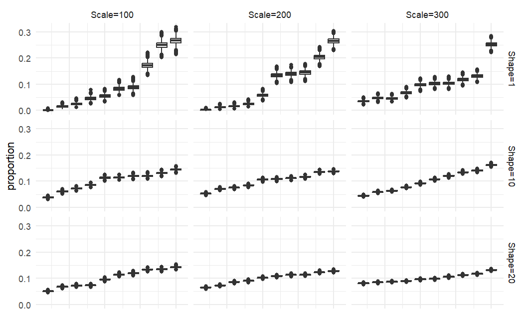
Figure 4. For each of nine different combinations of shape and scale parameters of a Gamma distribution a set of concentration parameters is generated for ten establishments. With each set of concentration parameters, the corresponding proportions are generated over 10,000 replications.

Using month 1 and 3 employment values from the Dirichlet Divider, month 2 employment is generated with Algorithm 2 and noise parameter $0.5$. The state and higher levels of industry codes can be extracted from the county and NAICS-6 codes. In Table 4, five variables take constant values in our synthetic QCEW data. We complete the generation of the synthetic establishment dataset by adding these constant-valued variables to the dataset.

Input: cntyN6.m1emp, cntyN6.m3emp, cntyN6.wage, cntyN6.estnum ;

/* From Algorithm 5 output */

1

$\eta>0$ ;

/* noise parameter for m2emp */

2

$\alpha_{prior},\theta_{prior}$;

/* shape and scale parameters for the Dirichlet prior respectively */

3

$n=0$ ;

/* initialize index for establishments */

4foreach $(c,\ell)\in\texttt{cntyN6}$ do

5   $d\leftarrow\texttt{cntyN6.estnum}_{c,\ell}$;

6   $\mathbf{a}=(a_{1},\dots,a_{d})$ where $a_{j}\overset{i.i.d.}{\sim}\operatorname{Gamma}(\alpha_{prior},\theta_{prior})$;

7   $\texttt{m1emp}_{n+1},\dots\texttt{m1emp}_{n+d}\leftarrow\text{Dirichlet Divider}(\mathbf{a},\texttt{cntyN6.m1emp})$ where Dirichlet Divider is Algorithm 6;

8   $\texttt{m3emp}_{n+1},\dots\texttt{m3emp}_{n+d}\leftarrow\text{Dirichlet Divider}(\mathbf{a},\texttt{cntyN6.m3emp})$ ;

9   $\texttt{wage}_{n+1},\dots\texttt{wage}_{n+d}\leftarrow\text{Dirichlet Divider}(\mathbf{a},\texttt{cntyN6.wage})$ ;

10   $\texttt{cnty}_{n+j}=c$ for $j=1,\dots,d$;

11   $\texttt{naics}_{n+j}=\ell$ for $j=1,\dots,d$;

12   $\texttt{primary\_key}_{n+j}=n+j$ for $j=1,\dots,d$;

13   $\texttt{m2emp}_{n+j}\leftarrow\text{Month 2 Employment}(\eta,\texttt{m1emp}_{n+j},\texttt{m3emp}_{n+j})$ for $j=1,\dots,d$ where Month 2 Employment is Algorithm 2;

14   $n=n+d$;

/* fill in other variables from naics and cnty values */

15foreach $\texttt{id}\in\texttt{primary\_key}$ do

16   Extract $\texttt{supersector}_{\texttt{id}},\texttt{sector}_{\texttt{id}},\texttt{naics3}_{\texttt{id}},\texttt{naics4}_{\texttt{id}},$ and $\texttt{naics5}_{\texttt{id}}$ from $\texttt{naics}_{\texttt{id}}$;

17   Extract $\texttt{state}_{\texttt{id}}$ from $\texttt{cnty}_{\texttt{id}}$;

18   Set constant-valued variables $\texttt{year}_{\texttt{id}}=2016,~\texttt{qtr}_{\texttt{id}}=1,~\texttt{own}_{\texttt{id}}=5,\texttt{can\_agg}_{\texttt{id}}="Y",$ and $\texttt{rectype}_{\texttt{id}}="C"$

Result: dataset with a row for each primary_key and columns for each variable from Table 4

Algorithm 7 (Employment and Wages Microdata) This algorithm uses the Dirichlet Divider (Algorithm 6 and the Month 2 Employment (Algorithm 2 to generate synthetic establishment-level monthly employment and quarterly wage values based on the output from County by NAICS-6 (Algorithm 5). Then from the NAICS-6 code and county code the remaining variable described in Table 4 are generated.

Potential improvements to this method would be to utilize the size class information from the CBP data to inform the generation of monthly employment values at the establishment level. Additionally, a more sophisticated imputation technique could be employed rather than simulating from regression models. The regression models could also be improved by incorporating more publicly-accessible county-level data or by using more subject-area informed variable selection.

Appendix B An additional result for QCEW

In Section 8.1, the quartiles and mean difference between the sanitized and original aggregate cell values for six aggregation levels are reported (Table 3). For a more complete picture of the distribution, the corresponding boxplots for four of these aggregation levels are include in Figure 5.

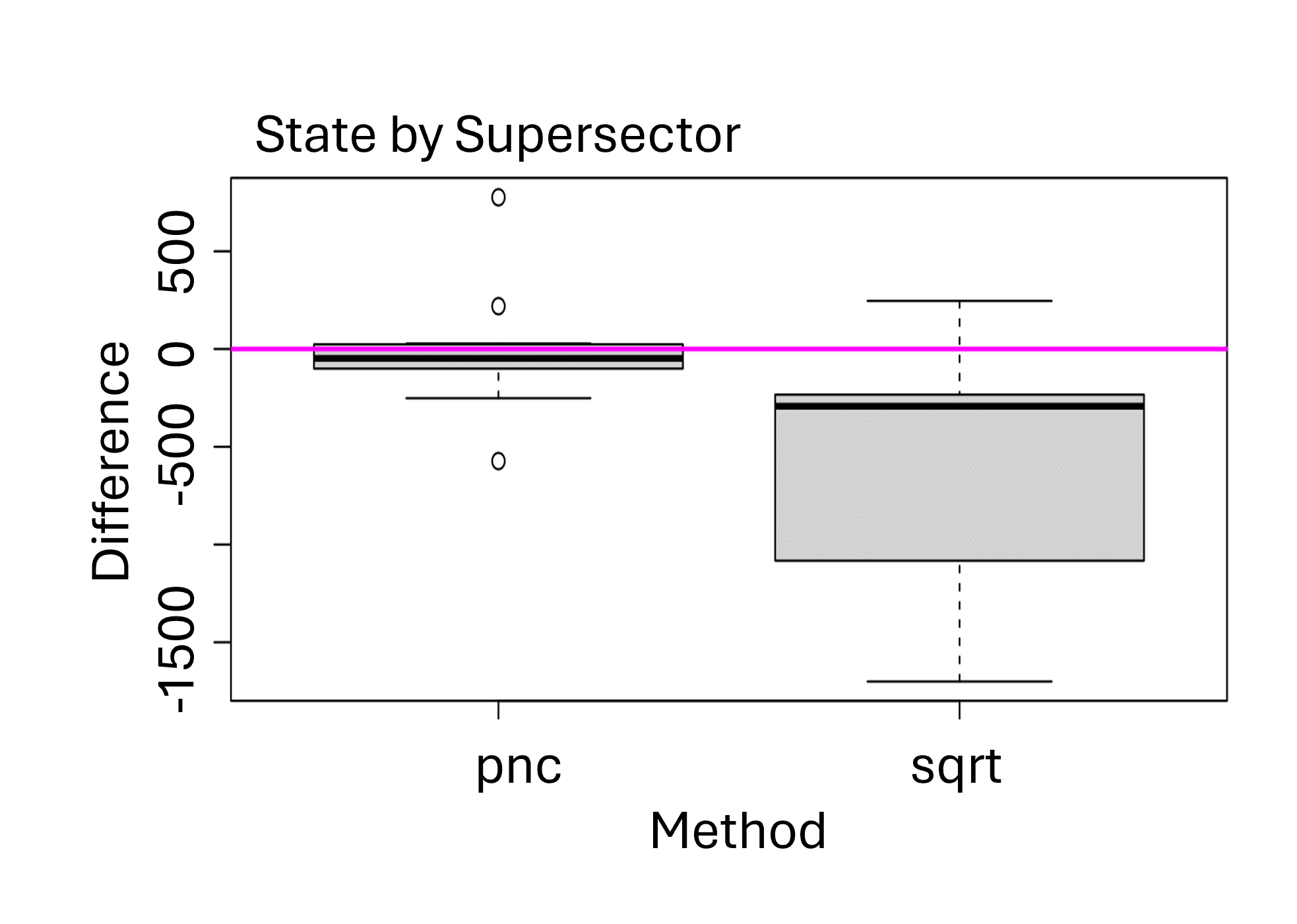
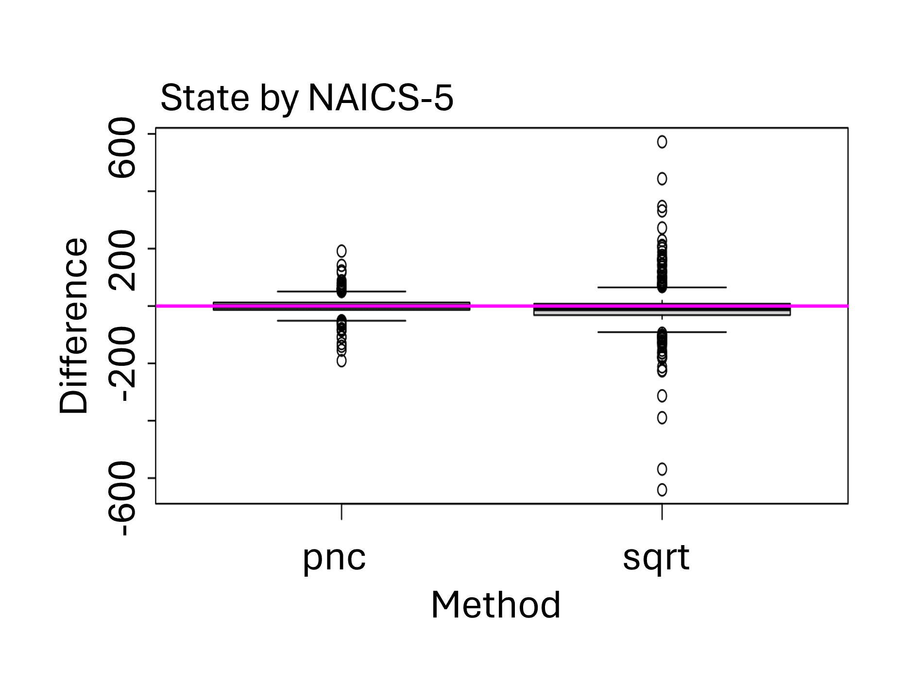
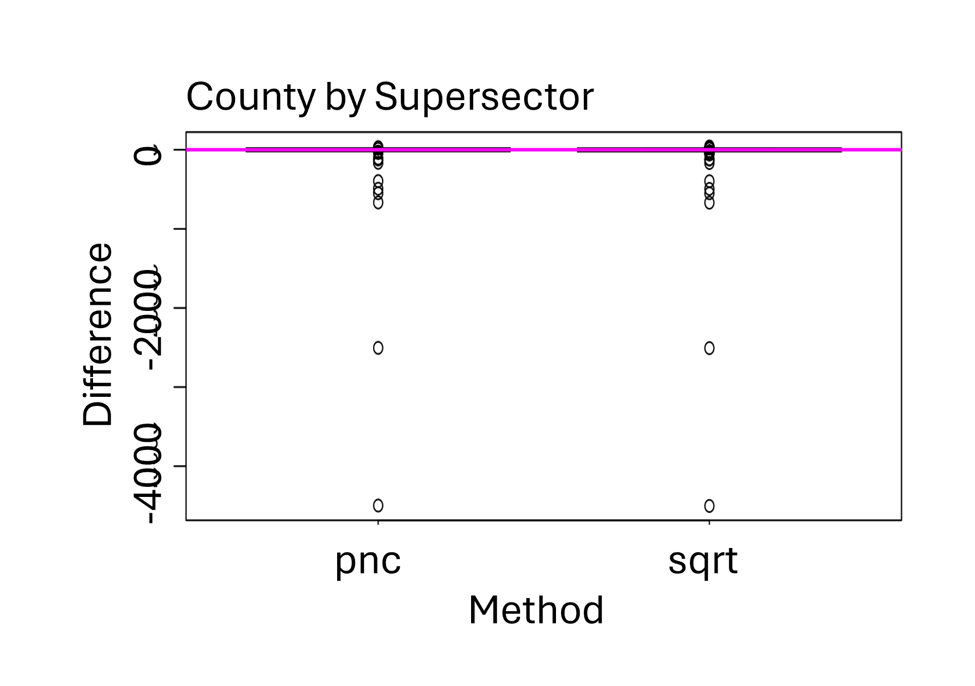
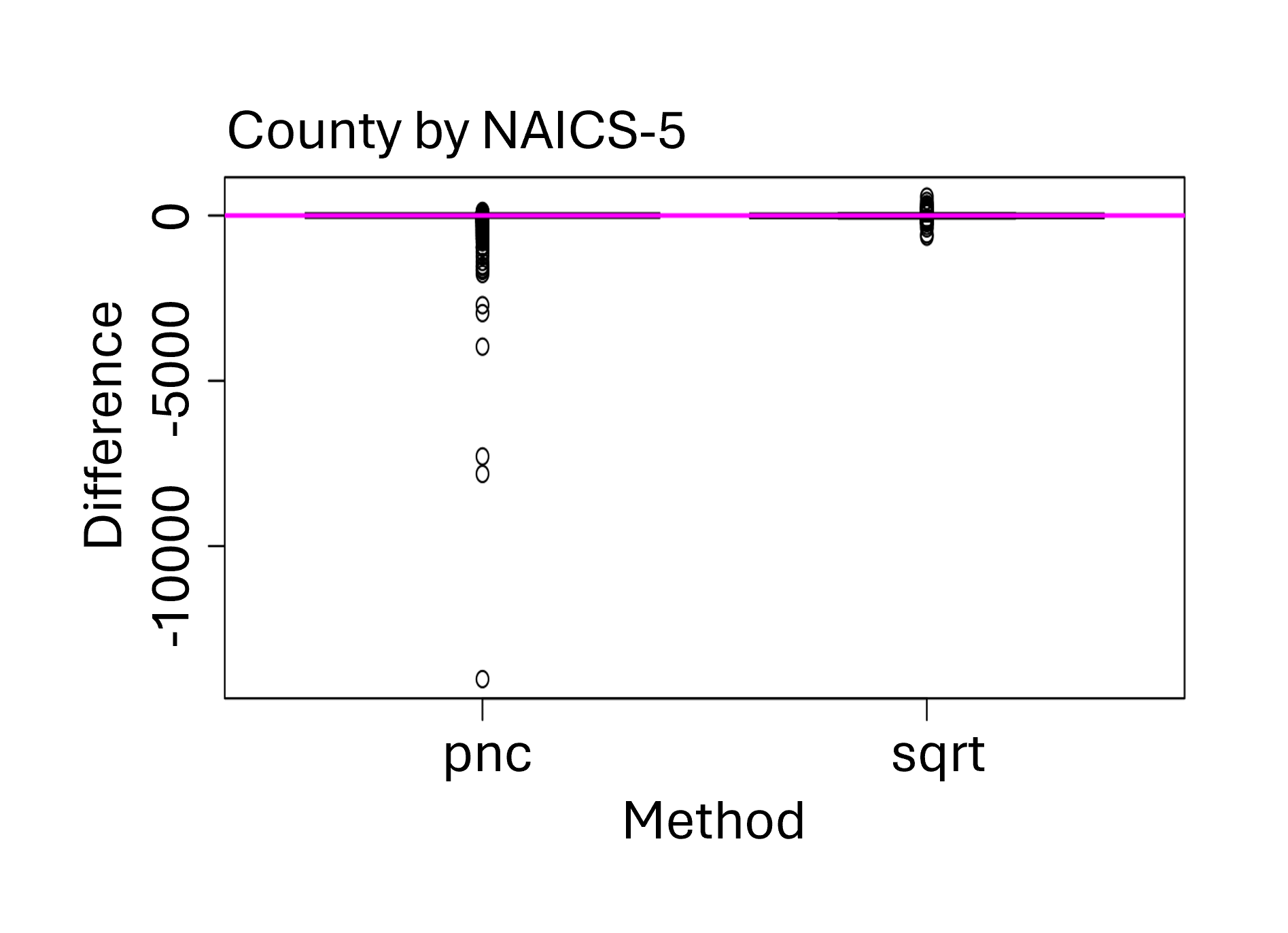
Figure 5. Comparison of the differences of the output from the two disclosure limitation methods and the original values for the state at different levels of aggregation. Going from left to right we cansee the distribution of the difference for the totals of cells by super-sector (aggregation level 53),5-digit NAICS (aggregation level 57), super-sector by county (aggregation level 73), and 5-digit NAICS by county (aggregation level 57).

We can also compare what happens when groupings get more fine-grained.Figure 6 shows boxplots (median, 1st and 3rd quartile, and outliers) of the signed differences for the group by queries “3-digit NAICS prefix” (left) and “3-digit NAICS prefix within each county” (right). Thus, each group in the right-most plot (all establishments with the same 3-digit NAICS prefix) gets subdivided in the left-most plot (a group consists of all establishments in the same county having the same 3-digit NAICS prefix). Figure 6 shows high utility (the quartiles and median are near 0), except for the outliers caused by confidentiality concerns as explained above. By comparing to Figure 1, we see that outliers are caused when the true employment total within a group is small (and hence would raise confidentiality problems if the answer in such a group was too accurate, especially if the group only had 1 establishment). For this reason, plots of confidentiality-preserving vs. true value (e.g., Figure 1) appear to be more informative than the distribution of raw differences across groups (e.g., Figure 6) as they present context that is not present in Figure 6.

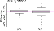
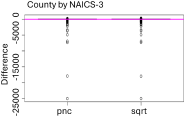
Figure 6. (Employment) Box-plot of signed difference for group-by 3-digit NAICS prefix (left) vs. group-by county and 3-digit NAICS prefix (right). Box-plots show median, 1st and 3rd quartiles, and the outliers. Both plots show downward bias. Median and quartiles for the right plot are all near 0.

Appendix C Error Tables from Synthetic Evaluation data

$q$	Query	$\mu_{q}$	$\mu_{q}^{2}/\mu^{2}$	$\mu_{q,e}$	$\mu_{q,w}$	$\mu_{q,w}^{2}/\mu_{q}^{2}$
$I$	Identity	1.22	.281	0.70	0.15	.015
$\Sigma$	State Total	0.36	.024	0.20	0.10	.077
$N5$	State NAICS-5	1.05	.207	0.60	0.15	.020
$C$	County Total	1.05	.207	0.60	0.15	.020
$C\text{x}N5$	County by NAICS-5	1.22	.281	0.70	0.15	.015

Table 7. The baseline privacy loss budget allocation to queries. The overall privacy budget $\mu\approx 2.31$ is allocated to five queries. The query level budget is denoted $\mu_{q}$ for query $q$. Within each query $q$, the budget is allocated to each month’s employment (denoted $\mu_{q,e}$) and quarterly wage (denoted $\mu_{q,w}$). Columns with headings $\mu_{q,e}$ and $\mu_{q,w}$ are exact values; everything else is computed from them using the composition rule (square root of the sum of squares) and rounded.

For our experiments, we focus on synthetic data for New Jersey and look at error metrics for quarterly wage and month 3 employment level query values. The creation of this synthetic dataset is described in Section A. We use two additional utility metrics in the appendix: absolute difference and relative absolute difference. We define absolute difference as $|x-\widetilde{x}|$ where $x$ is a confidential cell value of a query and $\widetilde{x}$ is the corresponding sanitized cell value. The relative absolute difference is the absolute difference scaled by the original value (i.e. $|x-\widetilde{x}|/(x+1)$). When we summarize the utility of cells across a query we use the mean for absolute difference and the median for the relative absolute difference. Median metrics are more robust to outliers than mean metrics so the combination of the two can be helpful to capture error behavior. However, the state total (51) and state by domain (52) queries only have one and two cells respectively, so these summary statistics should be identical in these cases. Additionally, we may be interested in how the distribution of the cell values within a query and the number of establishments aggregated into a cell will influence the utility of the queries. In Table 8 and Table 9, for each query we show the number of cells and some summary statistics for the number of establishments in each cell. The 3-,4-, and 5- digit NAICS codes at both the state and county level have a wide range of establishments per cell with a minimum of 1 and the maximum over 1,000. Most queries result in the standard deviation of establishments per cell that is larger than the mean number of establishments. All this suggests highly variable cells in terms of the number of establishments.

Synthetic New Jersey State-level Queries
	Min	Median	Max	Mean	Std.Dev.
State by Domain (52) has 2 cells
$n$	28476	103884	179292	103884	106643
$emp$	389796	1513961	2638126	1513961	1589809
$w$	56870451	65671540	74472630	65671540	12446620
State by Supersector (53) has 10 cells
$n$	250	22542	44429	20777	14141
$emp$	3457	236286	648521	302792	245261
$w$	1164792	5928548	51028965	13134308	16676271
State NAICS Sector (54) has 22 cells
$n$	67	5070	29073	9444	9538
$emp$	1261	97925	561919	137633	129971
$w$	34977	2829067	24074883	5970140	7101329
State NAICS 3-digit (55) has 74 cells
$n$	1	641	29073	2808	5253
$emp$	9	18359	298154	40918	61407
$w$	97	596856	19955782	1774906	3123361
State NAICS 4-digit (56) has 258 cells
$n$	1	144	16950	805	1716
$emp$	1	3679	200556	11736	21559
$w$	39	161771	9017144	509082	1250695
State NAICS 5-digit (57) has 571 cells
$n$	1	79	16950	364	1075
$emp$	1	1530	200556	5303	14205
$w$	39	40925	8276039	230023	747805
State NAICS 6-digit (58) has 853 cells
$n$	1	33	8172	244	692
$emp$	0	819	140800	3550	10231
$w$	0	21351	8276039	153978	591643

Synthetic New Jersey County Queries
	Min	Median	Max	Mean	Std.Dev.
County Total (71) has 21 cells
$n$	999	9385	28689	9894	6968
$emp$	15581	157835	370634	144187	103475
$w$	938253	5954245	16382122	6254432	5017341
County by Supersector (73) has 208 cells
$n$	1	676	6170	999	1069
$emp$	5	6844	99154	14557	18051
$w$	279	131295	9177485	631457	1344169
County NAICS Sector (74) has 454 cells
$n$	1	177	4146	458	638
$emp$	1	3280	77820	6669	9323
$w$	56	77536	8096919	289302	777652
County NAICS 3-digit (75) has 1324 cells
$n$	1	33	4146	157	348
$emp$	0	694	44129	2287	4458
$w$	5	13925	8096919	99202	440438
County NAICS 4-digit (76) has 3992 cells
$n$	1	12	2110	52	121
$emp$	0	209	28438	758	1704
$w$	0	3920	5935630	32902	201878
County NAICS 5-digit (77) has 8026 cells
$n$	1	7	2110	26	79
$emp$	0	84	25265	377	1159
$w$	0	1180	5935630	16365	137917
County NAICS 6-digit (78) has 10067 cells
$n$	1	5	1289	21	55
$emp$	0	63	25265	301	933
$w$	0	834	5929093	13047	120849

Table 8. Summary statistics for number of establishments in a cell ($n$), month 3 employment count ($emp$), and quarterly wages ($w$) for each aggregate level code for the synthetic New Jersey. Overall, synthetic New Jersey has 207,768 establishments.

Synthetic Rhode Island State-level Queries
	Min	Median	Max	Mean	Std.Dev.
State by Domain (52) has 2 cells
$n$	4439	12710	20981	12710	11697
$emp$	57050	188016	318981	188016	185213
$w$	5985933	5989127	5992321	5989127	4517
State by Supersector (53) has 10 cells
$n$	47	2994	4903	2542	1570
$emp$	297	34772	100286	37603	30426
$w$	64248	548588	5309640	1197825	1606737
State NAICS Sector (54) has 22 cells
$n$	14	687	3272	1155	1165
$emp$	111	14654	79298	17092	17778
$w$	35043	240442	3079880	544466	769112
State NAICS 3-digit (55) has 68 cells
$n$	4	109	2986	374	634
$emp$	8	2604	42028	5530	7873
$w$	104	73695	1250070	176151	247533
State NAICS 4-digit (56) has 224 cells
$n$	1	32	2409	113	227
$emp$	1	674	36147	1679	3292
$w$	27	19038	670281	53474	104387
State NAICS 5-digit (57) has 484 cells
$n$	1	16	2409	53	144
$emp$	1	200	36147	777	2278
$w$	1	4243	670281	24748	71079
State NAICS 6-digit (58) has 663 cells
$n$	1	10	1144	38	94
$emp$	1	147	20274	567	1617
$w$	1	2604	670281	18067	58239

Synthetic Rhode Island County Queries
Variable	Min	Median	Max	Mean	Std.Dev.
County Total (71) has 5 cells
$n$	1102	3354	14414	5084	5340
$emp$	10955	38191	237653	75206	92665
$w$	699819	1959523	4255187	2395651	1470599
County by Supersector (73) has 50 cells
$n$	1	274	2764	508	634
$emp$	1	2936	68784	7521	12431
$w$	1232	63424	2346055	239565	432476
County NAICS Sector (74) has 107 cells
$n$	1	104	1957	238	384
$emp$	1	1462	54369	3514	6694
$w$	87	25122	1314614	111946	241131
County NAICS 3-digit (75) has 303 cells
$n$	1	17	1698	84	197
$emp$	0	328	22958	1241	2834
$w$	0	6722	1175186	39532	109617
County NAICS 4-digit (76) has 854 cells
$n$	1	8	1323	30	73
$emp$	0	104	19551	440	1204
$w$	0	2232	510039	14026	48852
County NAICS 5-digit (77) has 1620 cells
$n$	1	4	1323	16	49
$emp$	0	42	19551	232	861
$w$	0	702	510039	7394	34446
County NAICS 6-digit (78) has 1996 cells
$n$	1	4	610	13	34
$emp$	0	35	12845	188	674
$w$	0	498	510039	6001	30892

Table 9. Summary statistics for number of establishments ($n$), employment count ($emp$), and quarterly wages ($w$) for each aggregate level code for the synthetic Rhode Island. Overall, synthetic Rhodes Island has 25,420 establishments.

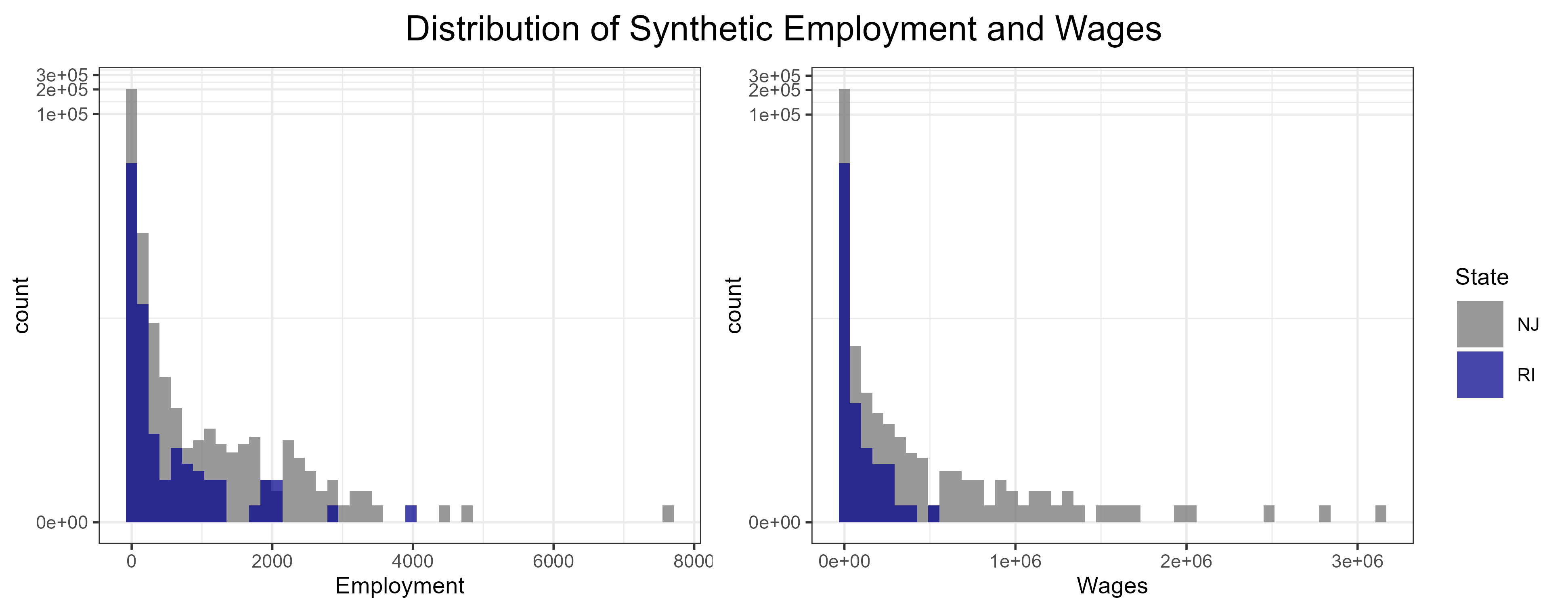
Figure 7. The distributions of wages and employment of the establishments in the Synthetic New Jersey and Rhode Island Datasets features a heavy tail. The skew of the data is so intense that the scale of the y-axis have to be transformed so the counts of the higher values bins are visible.

For all experiments, we use a baseline pnc-mechanism implementation with ${{\color[rgb]{0,0,0}\zeta}}=0.01$ and $\sqrt{\phantom{x}}$-mechanism implementation for comparison. This baseline matches the parameters used in Section 8. The baseline overall privacy budget is $\mu=2.31$ and the privacy distance for monthly employment is ${{\color[rgb]{0,0,0}\gamma}}_{emp}=0.5$ and for quarterly wages is ${{\color[rgb]{0,0,0}\gamma}}_{w}=50$. The baseline implementations use the queries and privacy parameters described in Table 7

Syn-NJ Employment:

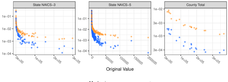
Syn-NJ Wages:

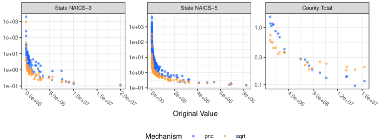
Figure 8. Comparison of pnc-mechanism in blue vs. $\sqrt{\phantom{x}}$-mechanism in orange on Synthetic NJ for employment and wages, using the baseline configuration from Table 7 ($\mu\approx 2.31$). The first column is the query that groups by 3-digit NAICS prefix (not a measurement query), while the other two columns evaluate accuracy on 2 measurement queries. $x$-axis: ground truth answer for a group, $y$-axis: corresponding relative error for that group.

When we vary privacy allocation with a fixed overall budget, we scale the privacy share of a query or confidential value type (i.e. wages or employment). This share is described as the squared ratio of the privacy cost to its next highest cost level. In other words, for query $k$ the wage privacy share is the squared privacy cost to wage ($\mu_{Q,w}^{2}$) over the query-level privacy budget ($\mu_{Q}^{2}$). For the baseline parameters this value is in the last column of Table 7. When we look at privacy allocation to queries, we look at the squared query budget $\mu_{Q}^{2}$ over the squared total budget $\mu^{2}$. For the baseline parameters, this is fourth column labeled $\mu^{2}_{Q}/\mu^{2}$ in Table 7.

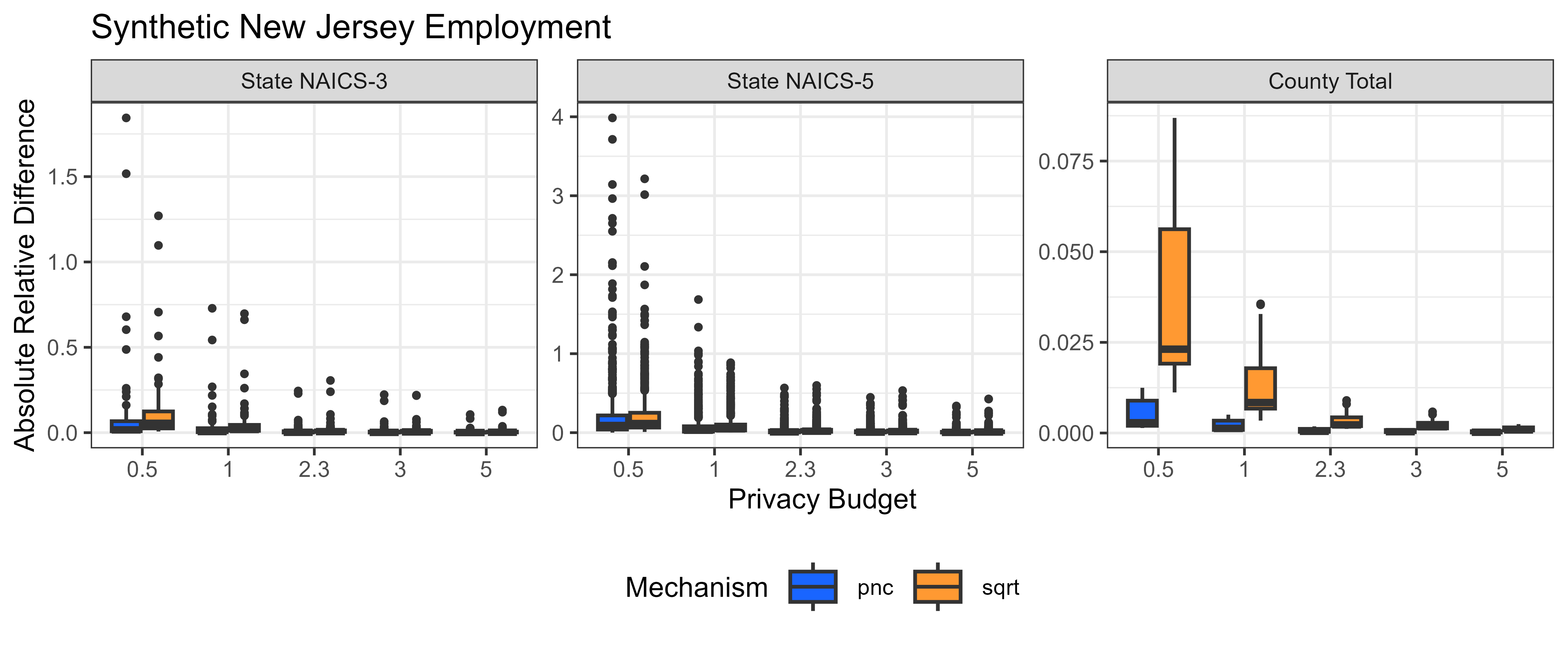
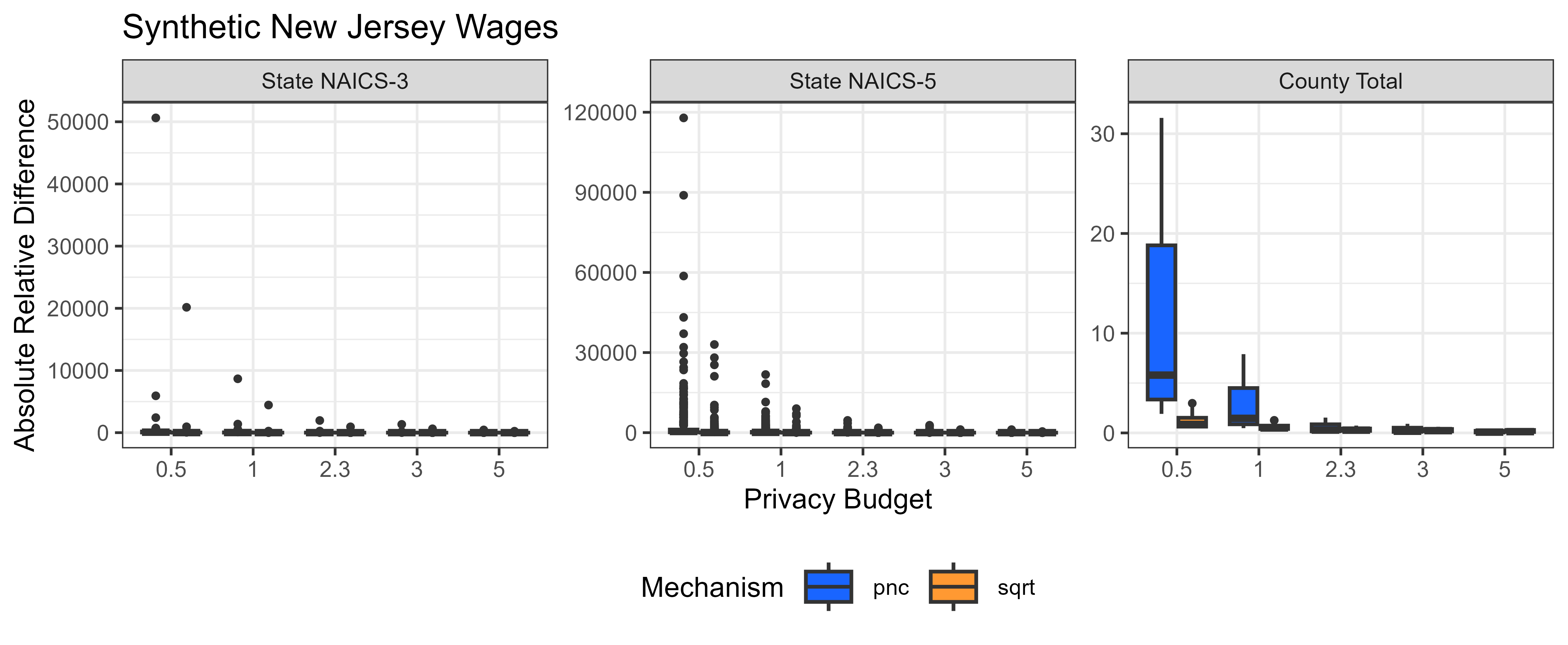
Figure 9. Employment and Wages relative errors, as overall privacy budget varies, using the base configuration from Table 7.

Appendix D Analyzing attacker error due to sampling.

The following example demonstrates why $\psi=\sqrt{}$ makes statistical sense and how it relates to estimating establishment count.

Example D.1.

Suppose an establishment ${{\color[rgb]{0,0,0}\mathcal{E}}}$ has $x$ employees and a statistician (e.g., an attacker or labor economist) wants to estimate its employment count.Suppose nearly all employees of ${{\color[rgb]{0,0,0}\mathcal{E}}}$ live within a region whose total population, $N$, is known with high accuracy (e.g., from Census data). For some $q\in[0,1]$, the statistician may take a random sample of $n=Nq$ people in the region and record the proportion $p$ that work for ${{\color[rgb]{0,0,0}\mathcal{E}}}$. The quantity $np$ can be modeled as the sum of $n$ Bernoulli$(x/N)$ random variables. So, an unbiased estimate of the number of employees of ${{\color[rgb]{0,0,0}\mathcal{E}}}$ is $\hat{x}=np(N/n)$. The variance of this estimate is $\operatorname{Var}(\hat{x})=n(x/N)(1-x/N)N^{2}/n^{2}=x\frac{N-x}{n}\leq\frac{1}{q}x$. The standard deviation is therefore $O(\sqrt{x})$ and confidence intervals would therefore have lengths $O(\sqrt{x})$.

Appendix E Discussion of Cell Suppression Weaknesses

Table 10. Establishment microdata and three marginals computed from it. Primary suppression must remove the cells for County X and Sector 52 (red), as they are directly revealing of the wages $\mathbb{B}$. Secondary suppression is needed to prevent $\mathbb{B}$ from being reconstructed by the remaining cells.

Establishment	County	Sector	Wages
Bob’s Building	X	52	$\mathbb{B}$
Carlos’s Construction	Y	23	$\mathbb{C}$
Green Hills Farming	Y	11	$\mathbb{G}$
Isaac’s Foundations	Z	23	$\mathbb{F}$
Alice’s Apples	Z	11	$\mathbb{A}$

Total Wages

$\mathbb{B}\!+\!\mathbb{C}\!+\!\mathbb{G}\!+\!\mathbb{F}\!+\!\mathbb{A}$

  By County X Y Z $\mathbb{B}$ $\mathbb{C}\!+\!\mathbb{G}$ $\mathbb{F}\!+\!\mathbb{A}$   By Sector 52 23 11 $\mathbb{B}$ $\mathbb{C}\!+\!\mathbb{F}$ $\mathbb{A}\!+\!\mathbb{G}$

Table 10 shows a simplified microdata set and 3 marginals computed from it: total wages, wages by county, and wages by sector (2-digit NAICS code) prefix. The values in cells for County X and also for Sector 52 (displayed in red) are directly disclosive because they only contain one establishment, and hence would undergo primary suppression.The secondary suppression phase then identifies which non-suppressed cells can be used to deduce the cells suppressed in the first phase, or can isolate additional establishments. For example, the total wages minus the combined wages of counties Y and Z, or total wages minus the combined wages of sectors 23 and 11 recover the wages $\mathbb{B}$. Meanwhile, the wages in counties Y and Z along with the wages in sectors 23 and 11 form a linear system of 4 equations and 4 unknowns and hence is uniquely solvable. A subset of these problematic cells needs to be suppressed with the goal that the remaining cells cannot be used to reconstruct sensitive values. Thus, for example, one could additionally suppress the total wages table, along with total wages of County Y. All that remains to be published are the wages of County Z, Sector 23, and Sector 11. In our example 50% of the cells end up being suppressed. This is not an anomaly. Primary and secondary suppression procedures results in the BLS suppressing the majority of the cells before they are released (U.S. Bureau of Labor Statistics, 2024a).

Appendix F Proofs from Section 5

Appendix G Proofs from Section 6

Several results in Section 6 rely on existing properties of Gaussian Differential Privacy (Dong et al., 2021) and adapt definitions associated with the GDP framework. The $\psi$-neighbor sensitivity (Definition 6.1) adapts $L_{2}$-sensitivity (Definition G.1) to our proposed framework.

Definition G.1 ($L_{2}$ sensitivity).

The $L_{2}$ sensitivity of a vector-valued function $q$ is defined as ${{\color[rgb]{0,0,0}{{\color[rgb]{0,0,0}\Delta}}_{2}}}(q)\equiv\sup_{{{\color[rgb]{0,0,0}\mathcal{D}}}_{1}\sim{{\color[rgb]{0,0,0}\mathcal{D}}}_{2}}||q({{\color[rgb]{0,0,0}\mathcal{D}}}_{1})-q({{\color[rgb]{0,0,0}\mathcal{D}}}_{2})||_{2}$, where the supremum is taken over all pairs of datasets that differ on the value of one record.

The ${{\color[rgb]{0,0,0}\psi}}$-neighbor sensitivity restricts the pairs of dataset to any which are ${{\color[rgb]{0,0,0}\psi}}$-neighbors (Definition 5.5) where as $L_{2}$-sensitivity considers all pairs of datasets differing on one record. Then the Estab-Gaussian mechanism in Definition 6.2 adapts the Gaussian Mechanism (Definition G.2) using the ${{\color[rgb]{0,0,0}\psi}}$-neighbor sensitivity (Definition 6.1).

Definition G.2 (Gaussian Mechanism (Dong et al., 2021)).

Let $q$ be a query represented by a vector-valued function. Given a privacy parameter $\mu$ and input dataset ${{\color[rgb]{0,0,0}\mathcal{D}}}$, the Gaussian Mechanism returns $q({{\color[rgb]{0,0,0}\mathcal{D}}})+N\left(0,\frac{{{\color[rgb]{0,0,0}{{\color[rgb]{0,0,0}\Delta}}_{2}}}^{2}(q)}{\mu^{2}}\mathbf{I}\right)$ and satisfies $\mu$-GDP.

Appendix H An Empirical Exploration of Bias Caused by Estimated Variances

For a simple, but illuminating scenario, consider a dataset with 100 counties and 2 establishments per county. To simplify interpretation of the outcome, set the ground truth to be 10 employees in each establishment. The queries of interest are the ID: the identity query (how many employees are in each establishment), County: the number of employees in each county, and Total: the total employment. In the first setting, we add noise to each query using $\psi$-mechanism with ${{\color[rgb]{0,0,0}\psi}}={{\color[rgb]{0,0,0}\sqrt{\phantom{x}}}}$ (${{\color[rgb]{0,0,0}\gamma}}=0.5$ and $\mu=1$); in the second setting, ${{\color[rgb]{0,0,0}\psi}}=\log$ (${{\color[rgb]{0,0,0}\gamma}}=0.1$ and $\mu=1$). In both cases, Theorem 6.6 is used to recover unbiased query answers. We consider 3 postprocessing strategies:

• Est: Postprocessing with Equation 1 using estimated variances.

• Act: (Non-privacy-preserving) ablation experiment using the true variances in Equation 1.

• Hybrid: (Non-privacy-preserving) ablation experiment that uses Equation1 with estimated variances for the ID query the true variances for the rest. By comparing to Act, we will see the effect of having exact variances for non-identity queries. The full recommended setup, using $\psi$-mechanism (with estimated variances) for the identity query and pnc-mechanism (whose exact variances are safe to release) will be studied in Section 8.

Table 11 shows that the impact of uncertain variances is significant – the total employment query, which often is the most important, has the most significant accuracy degradation (Est vs. Act columns). The effects are ameliorated when the true variance is unknown only for the identity query (Hybrid column). Hence, one should avoid mechanisms with non-releasable variance whenever possible.

	Ablation Setting, Reporting Mean Squared Errors
	$\mathbf{{{\color[rgb]{0,0,0}\psi}}={{\color[rgb]{0,0,0}\sqrt{\phantom{x}}}}}$			$\mathbf{{{\color[rgb]{0,0,0}\psi}}=\log}$
Query	Est	Act	Hybrid	Est	Act	Hybrid
ID	$7.5$	$7.6$	$7.5$	$18.0$	$23.7$	$19.2$
County	$10.5$	$10.0$	$10.1$	$40.0$	$37.9$	$35.0$
Total	$624.4$	$335.2$	$407.4$	$22,215.3$	$1,882.8$	$4,842.6$

Table 11. Postprocessing ablation study for evaluating the impact of using estimated variances with Equation 1. When ${{\color[rgb]{0,0,0}\psi}}={{\color[rgb]{0,0,0}\sqrt{\phantom{x}}}}$, then ${{\color[rgb]{0,0,0}\gamma}}=0.5,\mu=1$. When ${{\color[rgb]{0,0,0}\psi}}=\log$, then ${{\color[rgb]{0,0,0}\gamma}}=0.1,\mu=1$. Metric: mean-squared errors averaged over $1,000,000$ trials.

Appendix I Calculations from Section 7

References

- Abowd et al. (2021) John Abowd, Robert Ashmead, Ryan Cumings-Menon, Simson Garfinkel, Daniel Kifer, Philip Leclerc, William Sexton, Ashley Simpson, Christine Task, and Pavel Zhuravlev. 2021. An uncertainty principle is a price of privacy-preserving microdata. Advances in neural information processing systems 34 (2021), 11883–11895.
- Abowd et al. (2022) John M Abowd, Robert Ashmead, Ryan Cumings-Menon, Simson Garfinkel, Micah Heineck, Christine Heiss, Robert Johns, Daniel Kifer, Philip Leclerc, Ashwin Machanavajjhala, Brett Moran, William Sexton, Matthew Spence, and Pavel Zhuravlev. 2022. The 2020 census disclosure avoidance system topdown algorithm. Harvard Data Science Review 2 (2022).
- Adam and Worthmann (1989) Nabil R Adam and John C Worthmann. 1989. Security-control methods for statistical databases: a comparative study. ACM Computing Surveys (CSUR) 21, 4 (1989), 515–556.
- Brave et al. (2021) Scott A Brave, Charles Gascon, William Kluender, and Thomas Walstrum. 2021. Predicting benchmarked US state employment data in real time. International Journal of Forecasting 37, 3 (2021), 1261–1275.
- Bun and Steinke (2016) Mark Bun and Thomas Steinke. 2016. Concentrated differential privacy: Simplifications, extensions, and lower bounds. In Theory of cryptography conference. Springer, 635–658.
- Bureau (2024a) U.S. Census Bureau. (retrieved May 14, 2024)a. County Business Patterns 2016. https://www.census.gov/data/datasets/2016/econ/cbp/2016-cbp.html.
- Bureau (2024b) U.S. Census Bureau. (retrieved May 14, 2024)b. Quarterly Workforce Indicators 2016. https://ledextract.ces.census.gov/qwi/all.
- Casella and Berger (2002) George Casella and Roger L. Berger. 2002. Statistical Infence (2 ed.). Duxbury.
- Chatzikokolakis et al. (2013) Konstantinos Chatzikokolakis, Miguel E Andrés, Nicolás Emilio Bordenabe, and Catuscia Palamidessi. 2013. Broadening the scope of differential privacy using metrics. In 13th International Symposium (PETS).
- Cohen and Li (2006) Steve Cohen and Bogong T Li. 2006. A Comparison of Data Utility between Publishing Cell Estimates as Fixed Intervals or Estimates based upon a Noise Model versus Traditional Cell Suppression on Tabular Employment Data. https://www.bls.gov/osmr/research-papers/2006/pdf/st060100.pdf.
- Cox (1980) Lawrence H Cox. 1980. Suppression methodology and statistical disclosure control. J. Amer. Statist. Assoc. 75, 370 (1980), 377–385.
- Cox (1981) Lawrence H. Cox. 1981. Linear sensitivity measures in statistical disclosure control. Journal of Statistical Planning and Inference 5, 2 (1981), 153–164.
- Dalton et al. (2020) Michael Dalton, Elizabeth Weber Handwerker, and Mark A Loewenstein. 2020. Employment changes by employer size using the current employment statistics survey microdata during the COVID-19 pandemic. Covid Economics 46 (Sept. 2020), 123–136.
- Dong et al. (2021) Jinshuo Dong, Aaron Roth, and Weijie Su. 2021. Gaussian Differential Privacy. Journal of the Royal Statistical Society (2021).
- Dwork et al. (2006) Cynthia Dwork, Frank McSherry, Kobbi Nissim, and Adam Smith. 2006. Calibrating noise to sensitivity in private data analysis. In Theory of Cryptography: Third Theory of Cryptography Conference, TCC 2006, New York, NY, USA, March 4-7, 2006. Proceedings 3. Springer, 265–284.
- Eckert et al. (2020a) Fabian Eckert, Teresa C Fort, Peter K Schott, and Natalie J Yang. 2020a. County Business Patterns Database. https://doi.org/10.3886/E117464V1
- Eckert et al. (2020b) Fabian Eckert, Teresa C Fort, Peter K Schott, and Natalie J Yang. 2020b. Imputing Missing Values in the US Census Bureau’s County Business Patterns. Working Paper 26632. National Bureau of Economic Research. https://doi.org/10.3386/w26632
- Evans et al. (1996) Timothy Evans, Laura Zayatz, and John Slanta. 1996. Using noise for disclosure limitation of establishment tabular data. In Proceedings of the Annual Research Conference, US Bureau of the Census, Washington, DC, Vol. 20233. 65–86.
- Finley et al. (2024) Brian Finley, Anthony M Caruso, Justin C Doty, Ashwin Machanavajjhala, Mikaela R Meyer, David Pujol, William Sexton, and Zachary Terner. 2024. Slowly Scaling Per-Record Differential Privacy. arXiv preprint arXiv:2409.18118 (2024).
- Haney et al. (2017) Samuel Haney, Ashwin Machanavajjhala, John M Abowd, Matthew Graham, Mark Kutzbach, and Lars Vilhuber. 2017. Utility cost of formal privacy for releasing national employer-employee statistics. In Proceedings of the 2017 ACM International Conference on Management of Data. 1339–1354.
- Hay et al. (2009) Michael Hay, Vibhor Rastogi, Gerome Miklau, and Dan Suciu. 2009. Boosting the accuracy of differentially-private histograms through consistency. arXiv preprint arXiv:0904.0942 (2009).
- Holan et al. (2010) Scott H. Holan, Daniell Toth, Marco A. R. Ferreira, and Alan F. Karr. 2010. Bayesian Multiscale Multiple Imputation With Implications for Data Confidentiality. J. Amer. Statist. Assoc. 105, 490 (2010), 564–577. https://doi.org/10.1198/jasa.2009.ap08629
- Kifer and Machanavajjhala (2014) Daniel Kifer and Ashwin Machanavajjhala. 2014. Pufferfish: A framework for mathematical privacy definitions. ACM Transactions on Database Systems (TODS) 39, 1 (2014), 1–36.
- Kinney et al. (2011) Satkartar K Kinney, Jerome P Reiter, Arnold P Reznek, Javier Miranda, Ron S Jarmin, and John M Abowd. 2011. Towards unrestricted public use business microdata: The synthetic longitudinal business database. International statistical review 79, 3 (2011), 362–384.
- Lancaster (1969) H. O. Lancaster. 1969. The Chi-Squared Distribution. Hutchinston Educational.
- Li et al. (2015) Chao Li, Gerome Miklau, Michael Hay, Andrew McGregor, and Vibhor Rastogi. 2015. The matrix mechanism: optimizing linear counting queries under differential privacy. The VLDB journal 24 (2015), 757–781.
- Meer and West (2016) Jonathan Meer and Jeremy West. 2016. Effects of the minimum wage on employment dynamics. Journal of Human Resources 51, 2 (2016), 500–522.
- Nissim et al. (2007) Kobbi Nissim, Sofya Raskhodnikova, and Adam Smith. 2007. Smooth sensitivity and sampling in private data analysis. In Proceedings of the thirty-ninth annual ACM symposium on Theory of computing. 75–84.
- Pistner et al. (2018) Michelle Pistner, Aleksandra Slavković, and Lars Vilhuber. 2018. Synthetic data via quantile regression for heavy-tailed and heteroskedastic data. In International Conference on Privacy in Statistical Databases. Springer, 92–108.
- Resorts (2025) Disneyland Resorts. (retrieved June 20, 2025). Frequently asked questions about working at the Disneyland Resort. https://disneyexperiences.com/disneyland/our-cast/frequently-asked-questions-about-working-at-the-disneyland-resort/.
- Rockafellar (2015) Ralph Tyrell Rockafellar. 2015. Convex analysis:(pms-28). (2015).
- Sadeghi and Cooksey (2021) Akbar Sadeghi and Kevin Cooksey. 2021. Business employment dynamics by wage class. Monthly Lab. Rev. 144 (2021), 1.
- Sadeghi et al. (2016) Akbar Sadeghi, David M. Talan, and Richard L. Clayton. 2016. Establishment, firm, or enterprise: does the unit of analysis matter? Monthly Labor Review (2016). https://doi.org/10.21916/mlr.2016.51
- Salamon and Sokolowski (2005) Lester M Salamon and S Wojciech Sokolowski. 2005. Nonprofit organizations: New insights from QCEW data. Monthly Lab. Rev. 128 (2005), 19.
- Schmutte and Vilhuber (2020) Ian M Schmutte and Lars Vilhuber. 2020. Balancing privacy and data usability: An overview of disclosure avoidance methods. Handbook on Using Administrative Data for Research and Evidence-Based Policy (2020).
- Seeman et al. (2024) Jeremy Seeman, William Sexton, David Pujol, and Ashwin Machanavajjhala. 2024. Privately Answering Queries on Skewed Data via Per-Record Differential Privacy. Proc. VLDB Endow. 17, 11 (Aug. 2024), 3138–3150. https://doi.org/10.14778/3681954.3681989
- Smith and Thakurta (2022) Adam Smith and Abhradeep Thakurta. 2022. Fully Adaptive Composition for Gaussian Differential Privacy. https://doi.org/10.48550/ARXIV.2210.17520
- Toth (2014) Daniell Toth. 2014. Data smearing: an approach to disclosure limitation for tabular data. Journal of official statistics 30, 4 (2014), 839–857.
- Tran et al. (2023) Tran Tran, Matthew Reimherr, and Aleksandra Slavković. 2023. Differentially Private Synthetic Heavy-tailed Data. arXiv:2309.02416 [stat.AP]https://arxiv.org/abs/2309.02416
- U.S. Bureau of Labor Statistics (2024a) U.S. Bureau of Labor Statistics. (retrieved August 21, 2024)a. Handbook of Methods: Quarterly Census of Employment and Wages. https://www.bls.gov/opub/hom/cew/.
- U.S. Bureau of Labor Statistics (2024b) U.S. Bureau of Labor Statistics. (retrieved August 21, 2024)b. QCEW Public-Use Data Files. https://www.bls.gov/cew/downloadable-data-files.htm.
- U.S. Census Bureau (2024) U.S. Census Bureau. (retrieved August 21, 2024). North American Industry Classification System. https://www.census.gov/naics/.
- Washio et al. (1956) Yasutoshi Washio, Haruki Morimoto, and Nobuyuki Ikeda. 1956. Unbiased estimation based on sufficient statistics. Bulletin of Mathematical Statistics 6 (1956), 69–93.
- Webb et al. (2023) Kaitlyn Webb, Prottay Protivash, John Durrell, Daniell Toth, Aleksandra Slavković, and Daniel Kifer. 2023. Statistics-Friendly Confidentiality Protection for Establishment Data, with Applications to the QCEW. .
- Yang et al. (2011a) Y.M. Yang, A. Mushtaq, S. Pramanik, F. Scheuren, D. Hiles, M. Buso, and S. Butani. 2011a. Evaluation of Three Disclosure Limitation Models for the QCEW Program. BLS Research Papers https://www.bls.gov/osmr/research-papers/2011/pdf/st110120.pdf.
- Yang et al. (2011b) Y. Michael Yang, Ali Mushtaq, Santanu Pramanik, Fritz Scheuren, David Hiles, Michael Buso, and Shail Butani. 2011b. An Evaluation of BLS Noise Research for the Quarterly Census of Employment and Wages. BLS Research Papers https://www.bls.gov/osmr/research-papers/2011/pdf/st110120.pdf.