FPGA Design and Implementation of Fixed-Point Fast Divider
Using Goldschmidt Division Algorithm and Mitchell
Multiplication Algorithm

Abstract

This paper presents a variable bit-width fixed-point fast divider using Goldschmidt division algorithm and Mitchell multiplication algorithm. Described using Verilog HDL and implemented on a Xilinx XC7Z020-2CLG400I FPGA, the proposed divider achieves over 99% computational accuracy with a minimum latency of 99.1 ns, which is 31.7 ns faster than existing single-precision dividers. Compared with a Goldschmidt divider using a Vedic multiplier, the proposed design reduces Slice Registers by 46.68%, Slice LUTs by 4.93%, and Slices by 11.85%, with less than 1% accuracy loss and only 24.1 ns additional delay. These results demonstrate an improved balance between computational speed and resource utilization, making the divider well-suited for high-performance FPGA-based systems with strict resource constraints.

I Introduction

Hardware dividers implemented on field-programmable gate arrays (FPGAs) are critical components in many digital integrated circuit systems. Traditional fixed-point and floating-point dividers suffer from large computational latency and inflexible input bit-width. Function iteration methods provide an effective approach to improving divider performance. Among them, Newton–Raphson method [1] and Goldschmidt division algorithm [2] are widely adopted. Since the multiplications in Newton–Raphson method must be performed sequentially, while Goldschmidt algorithm achieves faster convergence with inherently parallel multiplications, the latter offers significant advantages in hardware implementations.

This paper proposes a variable bit-width fixed-point fast divider using Goldschmidt division algorithm and Mitchell multiplication algorithm [4]. By employing Mitchell algorithm in the multiplication units of the Goldschmidt iterations, the proposed divider achieves higher computational speed with modest accuracy loss, while maintaining relatively low resource utilization. Furthermore, the input and output bit-widths of the divider can be configured through parameters, enabling more flexible applications. Section II of this paper introduces the principles of Goldschmidt division algorithm and Mitchell multiplication algorithm. Section III presents the FPGA-based implementation of the proposed divider. Section IV provides the on-board operation results and performance analysis. Section V concludes the paper.

II The Principles of Algorithms

II-A Goldschmidt division algorithm

Goldschmidt division algorithm [2] is an iterative method based on multiplication and addition. Given a dividend $a$ and divisor $b$, the quotient is expressed as $q=a/b$. Letting $b=1-y$, the expression can be rewritten as:

$$q =\frac{a}{b}=\frac{a}{1-y}=\frac{a\left(1+y\right)}{\left(1-y\right)\left(1+y\right)}=\frac{a\left(1+y\right)\left(1+y^{2}\right)}{\left(1-y^{2}\right)\left(1+y^{2}\right)}$$

$$=\frac{a\left(1+y\right)\left(1+y^{2}\right)\cdots\left(1+y^{s}\right)}{1-y^{s}}.$$ (1)

From equation (1), if the convergence condition $b\in[1/2,1)$ is satisfied, the denominator $b_{s}=1-y^{s}$ approaches 1 as the iteration count $s$ increases, while the numerator $a_{s}=a(1+y)(1+y^{2})\cdots(1+y^{s})$ gradually converges to $q$. Based on this principle, the quotient can be approximated. At each iteration, the iteration coefficient is defined as $m_{s}=1+y^{s}=2-b_{s-1}$. The updated numerator and denominator are given by:

$$a_{s} =m_{s}a_{s-1},$$ (2a)

$$b_{s} =m_{s}b_{s-1}.$$ (2b)

The approximation accuracy of $a_{s}$ improves exponentially with $s$. The error between the approximate quotient $a_{s}$ and the exact quotient $q$ can be expressed by:

$$q-a_{s}\leq 2^{-2s}q.$$ (3)

Equation (3) indicates that after $s$ iterations, the precision of $a_{s}$ reaches $2^{s}$ bits. Each iteration of the Goldschmidt division algorithm involves only one subtraction and two parallel multiplications. Due to its fast convergence and parallelism, the algorithm enables high-speed division.

II-B Mitchell approximate multiplication algorithm

Mitchell multiplication algorithm [4] is an approximate binary multiplication method that replaces multiplication with addition. In traditional shift-based multipliers, both the number of computational steps and hardware resource usage increase with the growth of the input bit-width. In contrast, Mitchell algorithm maintains a fixed number of computational steps, thereby significantly improving multiplication speed while requiring relatively fewer hardware resources. This advantage becomes more obvious for long input bit-width, making this algorithm particularly suitable for constructing multipliers in Goldschmidt iteration units.

For a decimal number $N(N>1)$, its binary representation can be written as:

$$N=z_{k}z_{k-1}\cdots z_{1}z_{0}.z_{-1}z_{-2}\cdots z_{j},$$ (4)

where $z_{k}=1$. Thus, $N$ can be expressed as:

$$N=\sum_{i=j}^{k}2^{i}z_{i}=2^{k}\left(1+\sum_{i=j}^{k-1}2^{i-k}z_{i}\right)=2^{k}(1+x),$$ (5)

where

$$x=\sum_{i=j}^{k-1}2^{i-k}z_{i}=0.z_{k-1}z_{k-2}\cdots z_{j}.$$ (6)

In equation (6), $x$ corresponds to the fractional part of $N$ when $N$ is right-shifted by $k$ bits. Taking the base-2 logarithm on both sides of (5) and using the approximation $\log_{2}(1+x)\approx x$, we obtain:

$$\log_{2}N\approx k+x.$$ (7)

Accordingly, the multiplication of two non-negative real numbers $N$ and $M$ can be approximated as:

$$\log_{2}(NM)=\log_{2}N+\log_{2}M\approx k_{N}+k_{M}+x_{N}+x_{M}.$$ (8)

By applying the inverse transform of (5) and (7), the product $NM$ can be approximated as:

$$NM \approx 2^{k_{N}+k_{M}}(1+x_{N}+x_{M}),\ x_{N}+x_{M}<1$$ (9a)

$$NM \approx 2^{k_{N}+k_{M}+1}(x_{N}+x_{M}),\ \ \ x_{N}+x_{M}\geq 1$$ (9b)

Equations (9a) and (9b) represent the Mitchell multiplication without correction terms, where the maximum relative error is $1/9$. Its accuracy is insufficient for Goldschmidt iteration.

From equation (5), the precise product can be expressed as:

$$NM=2^{k_{N}+k_{M}}(1+x_{N}+x_{M}+x_{N}x_{M}).$$ (10)

Subtracting (9a) and (9b) from (10) respectively yields the correction terms:

$$(\ref{deqn_ex10})-(\ref{eq:9A}) =2^{k_{N}+k_{M}}(x_{N}x_{M}),\ \ x_{N}+x_{M}<1$$ (11a)

$$(\ref{deqn_ex10})-(\ref{eq:9B}) =2^{k_{N}+k_{M}}\left(x_{N}^{\prime}x_{M}^{\prime}\right),\ x_{N}+x_{M}\geq 1$$ (11b)

where $x_{N}^{\prime}=1-x_{N}$ and $x_{M}^{\prime}=1-x_{M}$. Adding the correction terms to (9a) and (9b), the exact product can be obtained. For hardware design convenience, let $k_{NM}$ be the integer part of $(k_{N}+k_{M}+x_{N}+x_{M})$, and $x_{NM}$ be the corresponding fractional part. Then, the exact product can be simplified without considering carry propagation:

$$NM =2^{k_{NM}}(1+x_{NM})+2^{k_{N}+k_{M}}(x_{N}x_{M}),\ x_{N}+x_{M}<1$$ (12a)

$$NM =2^{k_{NM}}(1+x_{NM})+2^{k_{N}+k_{M}}(x_{N}^{\prime}x_{M}^{\prime}),\ x_{N}+x_{M}\geq 1$$ (12b)

By recursively calculate the product terms $x_{N}x_{M}$ and $x_{N}^{\prime}x_{M}^{\prime}$ using (12a) and (12b), arbitrary precision of the product can be achieved. However, such nesting leads to excessive chip area consumption and computational latency. In practice, the correction terms are often approximated using (9a) or (9b), which reduces the maximum error to about 2.8% while preserving high calculation speed. Since the combined error behavior of Mitchell and Goldschmidt algorithms is difficult to analyses theoretically, error analysis for the proposed divider is provided in Section IV through empirical evaluation.

Additionally, although Mitchell algorithm can directly approximate the division by replacing addition with subtraction, the accuracy is limited to 87.5%, and no correction term can effectively improve the precision. Therefore, this approach is generally not adopted.

III FPGA-Based Implementation

III-A Overall Hardware Architecture

The overall hardware architecture of the proposed divider is shown in Fig. 1. It consists of an input sign converter, an iteration trigger, a finite state machine (FSM) controller, a data register, a normalization shifter, a Goldschmidt iteration unit, which incorporates Mitchell multiplier units and adders, as well as an output sign converter.

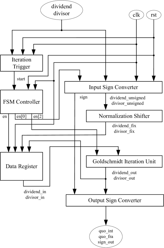
Figure 1: The overall hardware architecture of the proposed divider.

In Fig. 1, the dividend, divisor, clock signal (clk), and reset signal (rst) are the input signals. The signals dividend_unsigned and divisor_unsigned are the absolute value of dividend and divisor. The signal sign is the sign of the quotient. The signal start is the trigger signal initiating one division iteration. The signals en[3-0] are the enable signals. The signals dividend_fix, divisor_fix, dividend_out and divisor_out are the intermediate results of the iterations.

For convenience of description, the algorithm flow discussed in the following sections assumes that the enable signal en is active and rst is inactive. When the divisor is zero, the computation is considered invalid, and the output data is undefined.

III-B Input Sign Converter

The input signals dividend and divisor are signed integers, where the bit-widths are parameterized as $width\_dividend$ and $width\_divisor$, respectively. Their data formats are shown in Fig. 2.

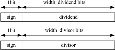
Figure 2: The data formats of input signals.

As shown in Fig. 3, the format of the input sign converter’s output is the unsigned fixed-point, in which the bit-width of the fractional part is defined by parameter $extension$, while the bit-width of the integer part is still $width\_dividend$ or $width\_divisor$. The same format is also employed for the intermediate results dividend_fix, divisor_fix, dividend_out and divisor_out.

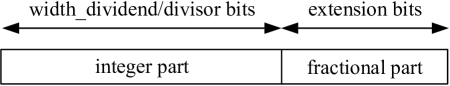
Figure 3: The data formats of internal signals.

The input sign converter is implemented using combinational logic, and its algorithm consists of the following steps:

• The input signals dividend and divisor are converted to their absolute value according to their sign bits, and output as dividend_unsigned or divisor_unsigned;

• The sign bits of dividend and divisor are XORed, and the result is output as the signal sign.

III-C Iteration Trigger

The iteration trigger is implemented using sequential logic. Its algorithm contains following steps:

• The input signals dividend and divisor are sent into two cascaded D flip-flops driven by the rising edge of clk, producing outputs dividend_1 and divisor_1, respectively;

• If dividend = dividend_1 and divisor = divisor_1, the output signal start is set to 0; otherwise, start is set to 1.

III-D FSM Controller

The FSM controller is implemented using sequential logic, and its state transition diagram is shown in Fig. 4. The number of iterations is set to four, which represents a trade-off between computational accuracy and latency. The FSM controller generates the enable signals en[3-0] (active-high) and controls the data flow of the data register, thereby governing the progress of the computation. The function of each bit of en is shown as follows:

• When en[0]=1, the input sign converter is enabled and stays ready while waiting for input data, then performs the sign conversion in the first clock cycle after data arrival;

• When en[1]=1, the adder calculates and outputs the iteration coefficient;

• When en[2]=1, the multiplier unit is enabled and performs the multiplication operation;

• When en[3]=1, the output sign converter outputs the final result.

Figure 4: The state transition diagram of the FSM controller.

III-E Normalization Shifter

The normalization shifter is implemented using combinational logic, and its algorithm can be summarized as the following steps:

• A flag signal (once) is initialized to 1, and the intermediate value $shift\_length\_R$ is initialized to 0;

• When the input signal divisor_unsigned changes, a loop is initiated. While once = 1, the bits of divisor_unsigned are checked sequentially from the most significant bit (MSB) to the least significant bit (LSB). If the current bit is 0, the value of $shift\_length\_R$ is added by 1. If the current bit is 1, the flag signal (once) is set to 0, then no further operations are performed in the remaining loop;

• Finally, divisor_unsigned is left-shifted by $(extension-width\_divisor+shift\_length\_R-1)$ bits to obtain divisor_fix, which falls within the interval [0.5,1). Then dividend_unsigned is left-shifted by the same amount to align with divisor_fix, yielding dividend_fix.

III-F Goldschmidt Iteration Unit

The iteration process of the Goldschmidt algorithm is illustrated in Fig. 5. For simplicity, $a$ and $b$ represent dividend_unsigned and divisor_unsigned, which are the output of the input sign converter. $a_{0}$ and $b_{0}$ represent dividend_fix and divisor_fix, which are the output of the normalization shifter. $m$ represents the iteration coefficient.

Since the proposed divider employs a data register to store intermediate results, the iteration unit can be reused across iterations. As a result, the hardware implementation requires only one adder and two multiplier units.

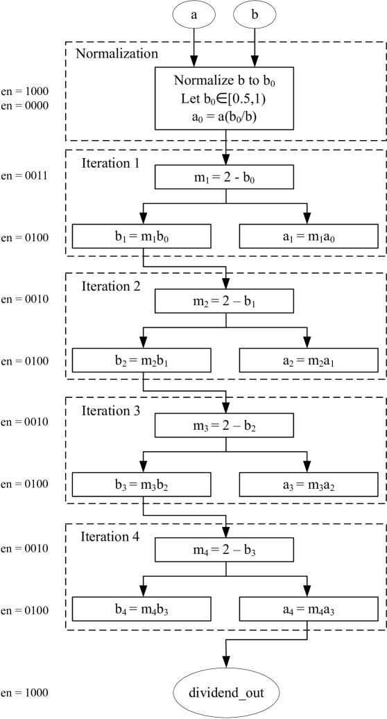
Figure 5: The iteration process of Goldschmidt algorithm.

Goldschmidt algorithm can be summarized as following steps:

• After normalization, the initial divisor $b_{0}$ is obtained within the interval [0.5,1). The initial dividend $a_{0}$ is obtained by aligning with $b_{0}$;

• In each iteration, the iteration coefficient $m_{k}$ is first computed, followed by parallel updates of the numerator and denominator;

• After four iterations, the value of $a_{4}$ is output as the approximate quotient.

III-G Data Register

The data register is implemented using sequential logic, triggered by the rising edge of clk. Its function is to store the intermediate results of the Goldschmidt iterations, including dividend_fix, divisor_fix, dividend_out, and divisor_out. Depending on the value of the enable signal en, the register selectively loads different intermediate data into dividend_in and divisor_in at different computation stages, which are then sent to the iteration unit for the subsequent iteration step.

The algorithm of the data register is illustrated in Fig. 6. Since the logic for the divisor is identical to that for the dividend, only the algorithm for the dividend is presented.

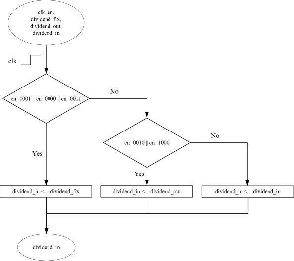
Figure 6: The algorithm of the data register.

III-H Mitchell Multiplier Unit

Based on the principles discussed in Section II, the Mitchell multiplier unit with correction, as illustrated in Fig. 7, is implemented using combinational logic and controlled by the signal en. Each multiplier unit consists of a primary multiplier, a correction multiplier, and two auxiliary shifters. Let the two operands be denoted as $N$ and $M$.

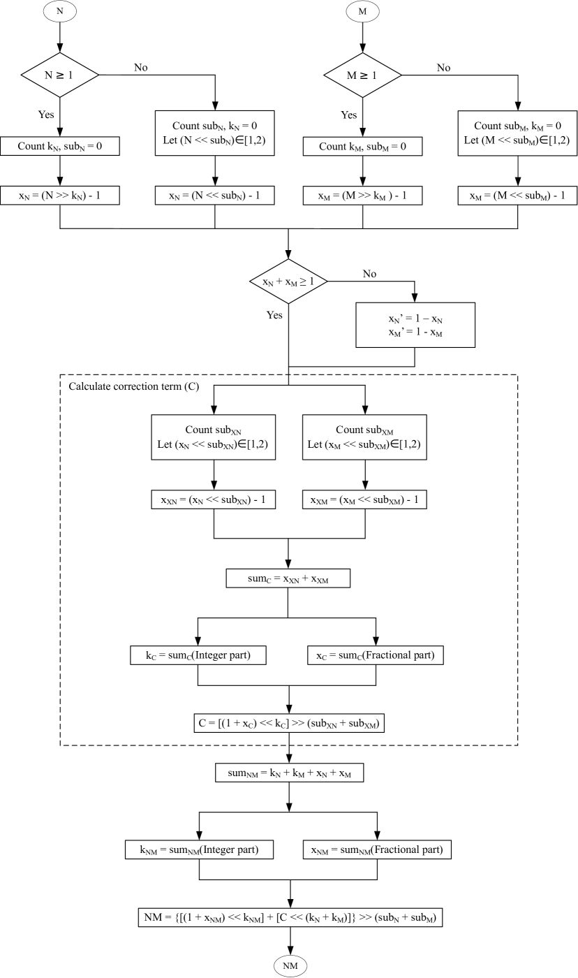
Figure 7: The algorithm of the Mitchell multiplier unit with correction.

It is important to note that the equations in Section II are valid only when both $N$ and $M$ are greater than 1. If either operand is less than 1, it should be left-shifted by $sub_{N}$ or $sub_{M}$ bits to ensure the values fall within the interval [1,2). After computation, the result is right-shifted by $(sub_{N}+sub_{M})$ bits to restore the correct magnitude.

The operations Count k and Count sub in Fig. 7 consist of the following steps:

• The operands $N$,$M$,$x_{N}$,$x_{M}$ are sent to the auxiliary shifters, which generate the corresponding $shift\_length$ values.

• The value of $k$ and $sub$ are then computed according to:

$$k=shift\_length-extension-1,$$ (13)

$$sub=extension-shift\_length+1.$$ (14)

During the computation of the correction term C, it is observed that $x_{N}$,$x_{M}$,$x_{N}^{\prime}$,$x_{M}^{\prime}$$<1$. Therefore, the branch of calculating $k$ can be omitted.

III-I Auxiliary Shifter

The auxiliary shifter is implemented using combinational logic. Let the two operands of the multiplication be denoted as num1 and num2. Its algorithm can be summarized as following steps:

• The algorithm of the normalization shifter is performed on the operands num1 and num2, obtaining the corresponding intermediate values $shift\_length\_num\_R\_1$ and $shift\_length\_num\_R\_2$;

• The value of $shift\_length\_num$ for each operand is calculated according to the following expression:

$$shift\_length\_num= width\_num+extension–$$

$$shift\_length\_num\_R+1.$$ (15)

Then $shift\_length\_num$ is sent to the multiplier for the subsequent calculation of $k$ and $sub$.

III-J Output Sign Converter

The final quotient of the divider is represented as a signed fixed-point number, as shown in Fig. 8. The bit-width of the integer part is defined by the parameter $width\_quo$, while that of the fractional part is defined by the parameter $(width\_fra-1)$.

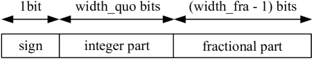
Figure 8: The data format of the final result.

The output sign converter is implemented using combinational logic. According to the signal sign, it converts the final iteration result dividend_out into the corresponding signed number, which is the final quotient. The final quotient is then partitioned into the integer part quo_int and the fractional part quo_fra, and they are output separately. Additionally, the sign bit of the quotient is also output as the signal sign_out.

IV On-Board Operation Results and Performance Analysis

The proposed divider is described in Verilog HDL and implemented on a Xilinx XC7Z020-2CLG400I FPGA. For on-board testing, the bit-width of input is configured to 32 bits (single-precision), and the quotient is output in signed fixed-point format with 32-bit integer and 32-bit fractional parts. Calculation examples and the corresponding error analysis are shown in Table I.

TABLE I: Calculation Examples and Error Analysis

Dividend	Divisor	Accurate Quotient	Computed Quotient	Relative Error(%)
$-17$	$35$	$-0.4857$	$-0.4868$	$0.22$
$53$	$11$	$4.8181$	$4.8253$	$0.14$
$345$	$4252$	$0.0811$	$0.0812$	$0.10$
$2741$	$67$	$40.9104$	$40.9342$	$0.05$
$34242$	$5567$	$6.1508$	$6.1759$	$0.40$
$89230293$	$432424$	$206.3490$	$206.7367$	$0.18$
$2^{31}-1$	$947483647$	$2.2665$	$2.2685$	$0.08$
$2^{31}-1$	$-47483647$	$-45.2257$	$-45.4989$	$0.60$

More than 100 tests were performed, confirming that the relative error of the computed quotient is below 1%.

The timing test was conducted using the FPGA’s Virtual I/O (VIO) core. For the input $53/11$, the waveform in Fig. 9 shows a total latency of 11 clock cycles from trigger to completion.

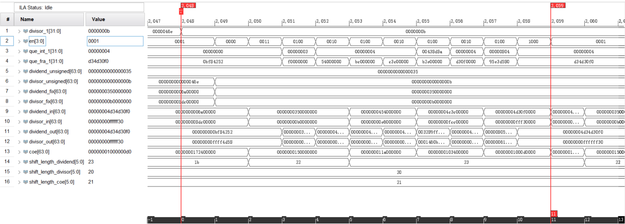
Figure 9: The waveform of the on-board calculation.

The Xilinx implemented power report of the proposed divider is shown in Table II.

TABLE II: An Example of a Table

Specifications	Values
Total On-Chip Power	$0.152W$
Junction Temperature	$26.7^{\circ}C$
Thermal Margin	$58.3^{\circ}C(4.9W)$
Effective $\theta JA$	$11.5^{\circ}C/W$

A comparison of latency and operating speed with existing dividers is presented in Table III.

TABLE III: An Example of a Table

Algorithm	Setup WNS(ns)	fmax (fmax= 1/(T-WNS)) (MHz)	Number of clock cycles required	Latency time(ns)
O-FixDiv[5]	$3.997$ $(@70MHz)$	$97$	$Q$	$10.289*Q$
RS-FixDiv[6]	$4.619$ $(@100MHz)$	$186$	$Q$	$5.381*Q$
FloatDiv[7]	$-$	$-$	$-$	$130.8$
Goldschmidt FloatDiv (Vedic) [3]	$-$	$-$	$-$	$75$
This work	$11.068$ $(@50MHz)$	$111$	$11$	$99.1$

Resource utilization comparison with another Goldschmidt-based divider [3], are shown in Table IV.

TABLE IV: An Example of a Table

	Slice Registers	Slice LUTs	Slices	BUFG
Ref. [3]	$3025$	$9281$	$2961$	$-$
This work	$1613$	$8823$	$2610$	$3$

The major drawback of existing fixed-point dividers [5], [6] is that the computation latency depends on the quotient Q. As Q increases, the required computation latency becomes longer, which introduces uncertainty and complicates the design of other modules that rely on the divider. In contrast, the minimum computation latency of the proposed divider is fixed at 99.1 ns, thereby avoiding the long-latency issue of dividers in [5] and [6] when Q is large. Furthermore, the proposed design achieves a speed advantage of 31.7 ns compared with the existing single-precision floating-point divider [7].

Within the same Goldschmidt algorithm framework, a comparison between the proposed divider using Mitchell multiplier units and the divider based on Vedic multiplier units [3] shows that the proposed divider reduces Slice Registers by 46.68%, Slice LUTs by 4.93%, and Slices by 11.85%, while the computation latency increases by only 24.1 ns and the relative error increases by less than 1%. Overall, the proposed divider achieves a more favorable trade-off between latency and hardware resource utilization.

V Conclusion

In this paper, a variable bit-width fixed-point fast divider using Goldschmidt division algorithm and Mitchell multiplication algorithm has been proposed, implemented, and tested on the Xilinx XC7Z020-2CLG400I FPGA platform. The proposed divider is designed with parameterized input and output bit-widths, which enables flexible application in different computational systems. On-board test results demonstrate that the proposed divider achieves more than 99% accuracy, with a minimum computation latency of 99.1 ns, which is 31.7 ns faster than the existing single-precision floating-point divider [7]. Compared with existing fixed-point dividers [5], [6], the proposed architecture achieves both shorter and fixed computation latency, eliminating the performance uncertainty associated with the value of the quotient. Furthermore, the proposed divider saves 46.68% Slice Registers, 4.93% Slice LUTs, and 11.85% Slices compared with the Goldschmidt divider using Vedic multiplier [3], at the cost of additional 24.1 ns latency and less than 1% relative error. The proposed divider is particularly well-suited for applications requiring high-speed computation with constrained hardware resources, such as image processing, industrial control, and Internet of Things (IoT) devices.

References

- [1] P. K. Pandey, D. Singh, and R. Chandel, ”Fixed-Point Divider Using Newton Raphson Division Algorithm,” in Proc. 5th Int’l Conf. Microelectron., Computing & Commun. Syst. (MCCS 2020), Ranchi, India, Jul. 2020, pp. 225-234, doi:10.1007/978-981-16 0275-7_19.
- [2] R. E. Goldschmidt, “Applications of division by convergence,” Ph.D. dissertation, Dept. Elect. Eng., Massachusetts Inst. Technol., Cambridge, MA, USA, 1964.
- [3] N. Singh and T. N. Sasamal, “Design and synthesis of goldschmidt algorithm based floating point divider on FPGA,” in Proc. 2016 Int. Conf. Commun. Signal Process. (ICCSP), Melmaruvathur, India, Apr. 2016, pp. 1286-1289, doi: 10.1109/ICCSP.2016.7754360.
- [4] J. N. Mitchell, “Computer Multiplication and Division Using Binary Logarithms,” IRE Trans. Electron. Comput, vol. EC-11, no. 4, pp. 512-517, Aug. 1962, doi: 10.1109/TEC.1962.5219391.
- [5] O. I. Bureneva and O. U. Kaidanovich, “FPGA-based Hardware Implementation of Fixed-point Division using Newton-Raphson Method,” in Proc. 2023 4th Int. Conf. Neural Netw. Neurotechnol. (NeuroNT), St. Petersburg, Russia, Jun. 2023, pp. 45-47, doi: 10.1109/NeuroNT58640.2023.10175844.
- [6] J. B, L. S. Kumar, A. Someshwaran, M. Sandya and N. Bharadwaj, “FPGA Implementation of Various Division Algorithms for Image Processing Applications - A Comparative Analysis,” in Proc. 2024 Int. Conf. Signal Process., Comput., Electron., Power Telecommun. (IConSCEPT), Karaikal, India, Aug. 2024, pp. 1-6, doi: 10.1109/IConSCEPT61884.2024.10627909.
- [7] K. Pande, A. Parkhi, S. Jaykar and A. Peshattiwar, “Design and Implementation of Floating Point Divide-Add Fused Architecture,” in Proc. 2015 5th Int. Conf. Commun. Syst. Netw. Technol. (CSNT), Gwalior, India, Apr. 2015, pp. 797-800, doi: 10.1109/CSNT.2015.179.