TRUST-Planner: Topology-guided Robust Trajectory Planner for AAVs with Uncertain Obstacle Spatial-temporal Avoidance

Abstract

Despite extensive developments in motion planning of autonomous aerial vehicles (AAVs), existing frameworks faces the challenges of local minima and deadlock in complex dynamic environments, leading to increased collision risks. To address these challenges, we present TRUST-Planner, a topology-guided hierarchical planning framework for robust spatial-temporal obstacle avoidance. In the frontend, a dynamic enhanced visible probabilistic roadmap (DEV-PRM) is proposed to rapidly explore topological paths for global guidance. The backend utilizes a uniform terminal-free minimum control polynomial (UTF-MINCO) and dynamic distance field (DDF) to enable efficient predictive obstacle avoidance and fast parallel computation. Furthermore, an incremental multi-branch trajectory management framework is introduced to enable spatio-temporal topological decision-making, while efficiently leveraging historical information to reduce replanning time. Simulation results show that TRUST-Planner outperforms baseline competitors, achieving a 96% success rate and millisecond-level computation efficiency in tested complex environments. Real-world experiments further validate the feasibility and practicality of the proposed method.

I Introduction

Currently, autonomous aerial vehicles (AAVs) play an increasingly crucial role in widespread areas, e.g., transportation, search and rescue, and sightseeing [1]. With the deepening of these applications, AAVs are required to operate in increasingly complex and dynamic flight environments, where moving obstacles, such as pedestrians, vehicles, and other AAVs, present growing risks of collision [2]. Therefore, ensuring both efficiency and safety in uncertain and dynamic environments still remains a significant challenge.

Motion planning navigates AAVs to traverse obstacles and reach their designated goals safely and quickly [3]. In general, it can be divided into two levels: high-level path planning and low-level trajectory planning. Path planning [4] mainly focuses on searching discrete geometric waypoints from start to goal. However, it usually neglects detailed dynamic constraints in exchange for better computation efficiency and global exploration ability, thereby limiting the full utilization of AAVs’ maneuverability. On the contrary, trajectory planning [5] considers practical differential dynamics, and generates continuous, smooth, and dynamically feasible motions. Trajectory planning is more closely integrated with the bottom-level flight control, and output commands can be accurately tracked and executed, thus providing better capabilities of real-time response and obstacle avoidance. Nevertheless, generating dynamically precise trajectories incurs sensitivity of initial guess and more computational burdens[6]. Consequently, the prevailing strategy is to integrate both by hierarchical planning frameworks [7], utilizing high-level path planning for global guidance and low-level trajectory generation for dynamic feasibility and real-time execution.

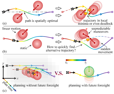
Figure 1: Main challenges of hierarchical motion planning in dynamic environments. (a) Structural spatial-temporal inconsistency. (b) Time-critical reconfiguration. (c) Lack of predictive foresight.

However, as illustrated in Fig.1, existing hierarchical planning frameworks still face significant challenges in dynamic environments, which can be summarized as follows:

1. Structural Spatial-temporal Inconsistency. Path typically contains discrete geometric points without explicit temporal information, while trajectory involves strong coupling of time and space. As a result of this structural inconsistency, although the guidance path is spatially feasible or even global optimal, the derived trajectory may be still trapped in local minima or even deadlock and collide in dynamic environments.

2. Time-critical Reconfiguration. Dynamic obstacles may exhibit unpredictably maneuvers or sudden movements. Without dedicated mechanisms for efficient management and rapid reconfiguration in emergency handling, existing frameworks often fail to promptly find and switch to alternative trajectory solutions, resulting in frequent abrupt stops and reduced flexibility.

3. Lack of Predictive Foresight. Existing frameworks often project dynamic environments on multiple stamps to simplify as static problems, and thus lack the predictive future foresight of obstacle avoidance from a spatial-temporal perspective. Thus, high-frequency replanning is required to cope with dynamic changes, imposing heavy computational burdens and higher collision risks.

Aim at these issues, we propose a Topology-guided Robust Planner for AAVs with Uncertain Obstacle Spatial-Temporal Avoidance (TRUST-Planner). Firstly, a dynamic enhanced visible PRM (DEV-PRM) frontend is proposed to capture approximate spatial-temporal topological characteristics in dynamic environments. Then, we present a uniform terminal-free minimum control polynomial (UTF-MINCO) backend, which utilizes the dynamic distance field (DDF) and relaxed terminal guidance strategy for efficient and flexible spatial-temporal avoidance with predictive foresight. Through the design of costs and derivation of analytical gradients, our backend transcribes the trajectory planning into a lightweight unconstrained optimization problem to achieve fast computation. Furthermore, an incremental multi-branch trajectory management framework is introduced. Through parallel computation and incremental replanning, it efficiently maintains the topological diversity of trajectories, enabling spatio-temporal topological decision-making for breaking the local minima and deadlock. Finally, extensive simulations and real-world experiments are presented to validate the efficiency, feasibility and practicality of the proposed method. The main contributions of this work are summarized as follows:

1. An efficient DEV-PRM topological path searching frontend is proposed. Compared to existing baseline [8], it improves the topological searching efficiency by 81.9% for more diversified topological guidance.

2. A lightweight trajectory optimization backend UTF-MINCO is proposed, which enables efficient dynamic obstacle avoidance with predictive foresight. Compared with existing methods [9], [10], [11], ours achieves 10 ms-level real-time trajectory optimization.

3. An incremental multi-branch trajectory management framework is introduced, which efficiently maintains the topological diversity using historical explored information and fast parallel optimization. Our framework outperforms baseline hierarchical planning frameworks [9], [8], achieving a 96% success rate in challenging complex dynamic and unknown environments.

II Related Works

II-A Hierarchical Planning Framework

Hierarchical planning have become a mainstream approach for motion planning in complex environments. The core idea is to decouple complex planning problems into several sublevels [12], such as “path$-$trajectory” bi-level frameworks [13], [9], and “path$-$corridor$-$trajectory” tri-level frameworks [14],[10] with flight corridors to enable safer planning in cluttered environments. This hierarchical decoupling significantly improves the computational efficiency and alleviates the initial sensitivity of single trajectory planning [15]. Unfortunately, it also introduces a structural defect of spatial-temporal inconsistency between different planning levels. As shown in Fig.1(a), this inconsistency can lead to local minima or even deadlock and collision, especially in dynamic environments. To alleviate this issues, researchers have attempted to introduce simplified kinematic [16], [9] or kinodynamic models [17], [18] into the path planning phase to provide coarse temporal information, while these approaches often come at the cost of reduced computational efficiency.

Addressing this structural challenge, this paper instead focuses on alternative approaches, namely topology-guided planning. These methods aim to find multiple different homotopic solutions in complex environments [19]. The concept of homotopy originally refers to the geometric classes with same topology that can be transformed by continuous deformation [20]. Interestingly, the homotopy of paths or trajectories means that they will lead to the same local minimum through continuous optimization [21]. Therefore, by searching diversity of homotopic solutions, the topology-guided approaches offer strong global exploration ability, and shows potential to break the spatial-temporal deadlocks and achieve flexible trajectory reconstruction. Researchers [8], [22], [23] have demonstrated the efficiency and robustness of topology-guided planning for quadrotors operating in cluttered environments. However, their approaches are developed for static scenarios and therefore lack foresight to handle spatial-temporal avoidance of moving obstacles, limiting their applicability in dynamic environments. Meanwhile, [24] and [2] explored topology-driven dynamic trajectory optimization framework, but their approaches is short of efficiently manage the known homotopies. As a result, they lose previously explored information during replanning, leading to reduced flexibility in trajectory reconstruction.

II-B Path Planning

Path planning generally include graph-based search [25], potential field [26], geometric-based methods [27], etc. However, these deterministic methods typically focus on finding a single solution, lacking the capability to explore multiple homotopies. By random sampling and multi-objective strategy, some sampling-based methods [28] and intelligent optimization [29] can obtain Pareto frontiers of feasible paths. Nevertheless, these multi-objective methods do not inherently guarantee the real-time solution of topologically distinct paths.

Currently, probabilistic roadmap (PRM) [30] and its variants [8], [2], [31], are the most widely used approaches for efficient topological path planning. PRM-based methods typically have a simple but effective architecture, which builds a roadmap by fast customized sampling (e.g. visible graph [8], [32]), and then uses homotopy checking (such as H-signature [21], visibility deformation (VD) [8], winding numbers[33]) to distinguish topological paths. However, most of them are restricted in dynamic environments, as they do not account for the obstacles motion. As a result, they can only capture spatial characteristics, limiting their ability to guide the spatio-temporal topological trajectories in dynamic environments.

II-C Trajectory Optimization

Trajectory planning, also known as trajectory optimization, is typically formulated as an optimal control problem (OCP), which aims to minimize a cost function (e.g. flight time [34] and control efforts [35]) subject to dynamics, terminal conditions and collision avoidance constraints. Such OCP is generally a strong nonlinear and nonconvex problem, and thus directly solving it by numerical optimization[36] or general solvers [11] is often time-consuming and intractable.

Owing to differential flatness of AAVs dynamics (e.g., quadrotors[35], fixed-wing[37], VTOL[38]), trajectory optimization can be transcribed into simple problems such as linear programming (LP) [9], quadratic programming (QP)[35], unconstrained optimization[10] for fast and efficient computation. The core of these differential flatness-based methods is lightweight trajectory representation, including polynomials[35], B-spline[17], Bézier [39] and other customized splines [10], [37]. Among them, minimum control polynomials (MINCO) [10] is a flexible and efficient representation with spatial-temporal deformability. However, MINCO relies on fixed terminal states, which limits its ability to handle uncertain or changing endpoints in dynamic environments. Moreover, as pointed out in [40], the nonuniform distribution of control points may also cause small obstacles to be missed.

Our trajectory planner is similar to [10] and [40], but has structurally improvement with relaxed terminals and inherent uniform control point distribution, enabling more flexible and safer trajectory adjustments in dynamic environments.

III Methodology

III-A Framework

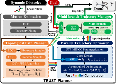
Figure 2: Framework of TRUST-Planner

As shown in Fig.2, TRUST-Planner comprises three key modules that work collaboratively to enable effective and safe navigation for AAVs in complex dynamic environments. These modules are detailed in Secs.III-B–III-D.

1. Multi-branch Trajectory Manager. This module serves as a customized container for trajectory management. Upon detecting environmental changes or task reconfiguration, the manager assigns replanning tasks to the path planner and trajectory optimizer, while continuously providing the optimal trajectory for drone navigation.

2. Topological Path Planner. We propose a Dynamic Enhanced Visible PRM (DEV-PRM) to capture approximate spatial-temporal topological characteristics in dynamic environments, which efficiently generates diverse, homotopy distinct paths for global guidance.

3. Parallel Trajectory Optimizer. The trajectory planning is formulated into a lightweight unconstrained optimization utilizing the proposed uniform terminal-free MINCO (UTF-MINCO) representation. The optimizer takes the topological paths as initial guidance, and generates multiple feasible trajectories by fast parallel computation.

III-B Multi-branch Topological Trajectory Management

Based on the concept of homotopic path [21] and trajectory [2], we first introduce the concept of the spatial-temporal homotopic trajectories as follows. Unlike [2], Definition 1 places greater emphasis on spatial-temporal characteristics, i.e., a trajectory may intersect with moving obstacles in space, but remains safe by avoiding them in both time and space.

  Definition 1 (Spatial-temporal homotopic trajectories).

For any two spatial-temporal trajectories $\tau_{1}(t)$, $\tau_{2}(t)\in\mathbb{R}^{3}\times\mathbb{R}$ with $t\in[t_{0},t_{f}]$, $\tau_{1}(t)$ is homotopic to $\tau_{2}(t)$ if there exists a continuous mapping $[t_{0},t_{f}]\times[t_{0},t_{f}]$. The trajectories in the same spatial-temporal homotopic class can be continuously deformed from one to another without crossing any obstacles at any time stamp $t\in[t_{0},t_{f}]$.

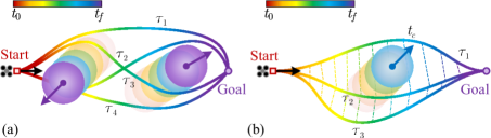
Figure 3: Illustration of spatial-temporal topologically trajectories. (a) Four trajectories $\tau_{1}$–$\tau_{4}$ belong to different spatial-temporal homotopy classes. (b) Temporal visibility deformation. $\tau_{1}$ and $\tau_{2}$ are in distinct homotopy because they are blocked by the moving obstacle at $t_{c}$, while $\tau_{2}$ and $\tau_{3}$ are equivalent.

Inspired by the uniform visibility deformation (UVD) in [8] for determining spatial homotopic of paths, as illustrated in Fig.3, we extended this idea to the spatial-temporal domain by employing the temporal visibility deformation (TVD) to identify the spatial-temporal homotopy of trajectories in dynamic environments. For two trajectories $\tau_{1}(t)$ and $\tau_{2}(t)$, we sample the time stamps $t_{c}$ and check whether they are blocked by the dynamic obstacles. They belong to the same spatial-temporal homotopy if and only if $\overrightarrow{\tau_{1}(t_{c})\tau_{2}(t_{c})}\cap\mathcal{O}(t_{c})=\varnothing,\,\forall t_{c}\in[t_{0},t_{f}]$. By comparing the visibility at these sampled instances, one can efficiently determine and separate the trajectories into different spatial-temporal homotopy classes.

Utilizing the TVD for spatial-temporal homotopy checking, we propose an incremental planning framework to manage multi-branch trajectory branches and enable efficient trajectory replanning, as shown in Algorithm 1. A customized queue with multiple different spatial-temporal topological trajectory branches is maintained, denoted as $\mathbb{T}=\{{\tau}_{0},{\tau}_{1},\ldots,{\tau}_{n-1}\}$. $\mathbb{T}$ is a priority queue with maximum $N$ branches, sorted by the cost values of the trajectories as $\mathcal{J}=\lambda_{t}\cdot\mathcal{H}_{t}+\lambda_{s}\cdot\mathcal{H}_{s}+\lambda_{e}\cdot\mathcal{I}_{e}$, where, $\mathcal{H}_{t}$ is the flight duration cost, $\mathcal{H}_{s}$ is the heuristic terminal cost, and $\mathcal{I}_{e}$ is the control efforts (detailed in Sec.III-D). The optimal trajectory ${\tau}_{0}$ is selected as the main branch for current navigation, while the others serve as sub-branches, providing a set of alternative safe trajectories for emergency situations.

Input: Start $\mathbf{p}_{s}$, goal $\mathbf{p}_{g}$, dynamic obstacles $\mathcal{O}(t)$

1 $t\leftarrow 0$, $\mathbf{p}(t)\leftarrow\mathbf{p}_{s}$;

2 while $\|\mathbf{p}(t)-\mathbf{p}_{g}\|\geq\varepsilon$ do // $\varepsilon$ is tolerance

3    $t\leftarrow t+\Delta t$;

4    Update $\mathbf{p}(t)$, $\mathcal{O}(t)$;

5    for each $\tau_{i}\in\mathbb{T}$ do

6       if $i=0$ then $\tau_{0}\leftarrow$ FwdMarch($\tau_{0}$, $\mathbf{p}_{g}$, $\mathcal{O}(t)$);

7       else $\tau_{i}\leftarrow$ BwdReplan($\tau_{i}$, $\mathbf{p}(t)$, $\mathcal{O}(t)$);

8      

9    end for

10   $\mathbb{T}_{\text{new}}\leftarrow$ FwdExplore($\tau_{0}$, $\mathbf{p}_{g}$, $\mathcal{O}(t)$);

11    for each $\tau_{j}\in\mathbb{T}_{\text{new}}$ do AddNewBranch($\mathbb{T}$, ${\tau}_{j}$);

12   

13 end while

14

150.1cm  

16 Function AddNewBranch($\mathbb{T}$, ${\tau}_{\text{new}}$):

17    isTopoNew $\leftarrow$ true;

18    for each $\tau_{i}\in\mathbb{T}$ do

19       if isTopoEqu(${\tau}_{i}$, ${\tau}_{\text{new}}$) then // by TVD

20          if $\mathcal{J}_{\text{new}}<\mathcal{J}_{i}$ then // better trajectory

21             ${\tau}_{i}\leftarrow{\tau}_{\text{new}},{\text{isTopoNew = false}}$;

22            

23          else return $\mathbb{T}$;

24         

25      

26    end for

27   if isTopoNew then $\mathbb{T}=\mathbb{T}\cup\{{\tau}_{\text{new}}\}$;

    $\mathbb{T}$.Sort() ;

    // by cost values

28    if $\mathbb{T}$.Size() $>$ $N$ then $\mathbb{T}$.PopBack();

29    return $\mathbb{T}$;

30   

31

Algorithm 1 Incremental Planning of TRUST-Planner

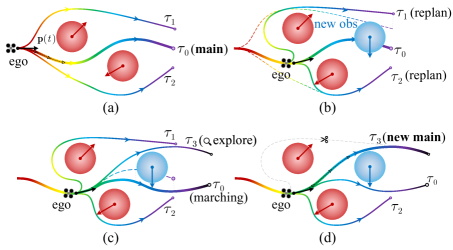
Figure 4: Incremental update process of topological trajectories. (a) The main branch $\tau_{0}$ publishes the setpoints for the drone’s navigation. (b) Replan of existing secondary branches $\tau_{1}$, $\tau_{2}$. (c) Forward planning of $\tau_{0}$, and topological exploration of new branches $\tau_{3}$. (d) Branches Decision. $\tau_{3}$ becomes the new main branch, while $\tau_{1}$ has been cut off.

With the ego heading towards the goal, dynamic obstacles also constantly moves. TRUST-Planner continuously monitors environmental changes and incrementally updates topological trajectory branches. As detailed in Sec.III-D, the trajectory planning is finally formulated into a lightweight problem with linear time and space complexity. Therefore, we employ parallel optimizers to efficiently and simultaneously update and reconstruct trajectories in real-time. Fig.4 illustrates the incremental update process of the trajectory branches, which involves three different types of trajectory replanning processes: 1) Forward marching of main branch, which extends the terminals of main trajectory towards the global goal $\mathbf{p}_{g}$; 2) Backward replanning of sub-branches, which aligns the start of sub-branches with the current state to enable the prompt and flexible switching as emergency requirements; and 3) Forward exploration of new homotopic branches, which explores the spatial-temporal topology of new environments and generates candidate trajectories for future navigation.

Summarily, the incremental replanning processes fully utilize the historical information of explored trajectories to efficiently maintain the topological diversity in the trajectory queue.

III-C Topological Path Planning

The topological path planning aims to explore the collision-free space in dynamic environments, and find diverse homotopy distinct reference paths, providing guidance for subsequent trajectory optimization. Inspired by [8], we propose a Dynamic Enhanced Visible PRM (DEV-PRM), which includes three key enhancements: 1) predictive obstacle modeling via the Predictive Directional Cone (PDC), 2) an obstacle-aware sampling strategy that improves initialization, and 3) a relaxed terminal constraint using the Goal Guidance Surface (GGS). These modifications are detailed as follows.

III-C1 Predictive Directional Cone (PDC)

Traditional path planning approaches lack explicit temporal information and do not account for obstacle motion uncertainty during the planning phase, thus they pose the challenge of spatial-temporal inconsistency. To address this issue, we project the predicted obstacle motion and its uncertainty into the spatial domain to incorporate temporal information into the path planning phase. A conservative geometric approximation, i.e., the Predictive Directional Cone (PDC), is constructed over a short time horizon to enable simplified and robust collision checking.

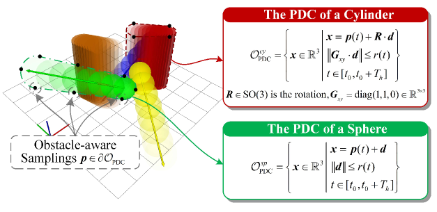
Figure 5: Illustration of predictive directional cones (PDCs) and obstacle-aware samplings.

As shown in Fig.5, given a dynamic obstacle $\mathcal{O}$, with intrinsic geometric size $r_{o}$, observed position ${\bf p}_{o}\in\mathbb{R}^{3}$, and velocity ${\bf v}_{o}\in\mathbb{R}^{3}$ at current time $t_{0}$. Its future motion is ${\bf p}_{o}(t)={\bf p}_{o}+{\bf v}_{o}\cdot(t-t_{0})+\delta(t)$, where $\delta(t)$ denotes the uncertainty maneuver item. Over a short prediction horizon $T_{h}$, assume that $\delta(t)$ is linear bounded and $\|\delta(t)\|\leq\mu_{o}\cdot(t-t_{0})$, where $\mu_{o}$ is the slope coefficient. Then, the uncertainty of the obstacle motion can be projected as the expansion of its geometric size $r_{o}(t)=r_{o}+\mu_{o}\cdot(t-t_{0})$. Therefore, the PDC $\mathcal{O}_{\text{PDC}}$ can be defined as the union of expanding cross-sectional volumes along the ${\bf v}_{0}$ direction as

$$\mathcal{O}_{\text{PDC}}=\bigcup\mathcal{O}[{\bf p}_{o}(t),r_{o}(t)],t\in[t_{0},t_{0}+T_{h}]$$ (1)

where $\mathcal{O}_{\text{PDC}}({\bf p},r)$ denotes the transformation of the base shape $\mathcal{O}$ with a translation by ${\bf p}-{\bf p}_{o}$, and a geometric scaling by $\frac{r}{r_{o}}$. Equation (1) a conservative spatial estimate of obstacle occupancy over a short horizon, while implicitly encoding the time characteristics of obstacle motion to support spatial-temporal topological exploration in path planning phase.

III-C2 Obstacle-Aware Sampling Strategy

Since the approximate motion information of dynamic obstacles has been encoded in PDCs, we can precompute a set of obstacle-aware samples $\mathcal{P}_{\text{PDC}}$ to guide the initialization of the topological roadmap as $\mathcal{P}_{\text{PDC}}=\{{\bf p}\in\partial\mathcal{O}_{\text{PDC}}\}$, where $\partial\mathcal{O}_{\text{PDC}}$ denotes the surface of $\mathcal{O}_{\text{PDC}}$. These samples are selected on multiple slices along the predicted velocity direction ${\bf v}_{0}$, capturing the spatial spread of potential future occupancy. The obstacle-aware samples $\mathcal{P}_{\text{PDC}}$ are inserted before the random sampling phase to initialize DEV-PRM, enhancing the roadmap’s ability to capture spatial-temporal topological structures.

III-C3 Goal Guidance Surface (GGS)

In the original V-PRM framework [8], the topological paths tend to directly connect with a fixed local goal, resulting in undesired lateral zigzagging motions toward the goal, thereby degrading the global optimality of the resulting trajectories. To address this issue, the Goal Guidance Surface (GGS) technique is introduced. As shown in Fig.6, instead of connecting to a fixed point, GGS replaces the local goal with a heuristic reference surface as

$$\mathcal{S}_{\text{GGS}}=\{{\bf p}\in\mathbb{R}^{3}\mid\|{\bf p}-{\bf p}_{g}\|_{2}=r_{\text{des}}\}$$ (2)

where ${\bf p}_{\text{goal}}$ represents the global goal position, and $r_{\text{des}}$ is the desired cut-off radius. Equation (2) defines a spherical surface that maintains a constant distance from the global goal. During the sampling process, the GGS acts as a special guard node, guiding local planning towards the global goal and mitigating lateral zigzagging behaviors. It gradually shrinks into a single point as the drone approaches the global goal, naturally degenerating into the original behavior of V-PRM.

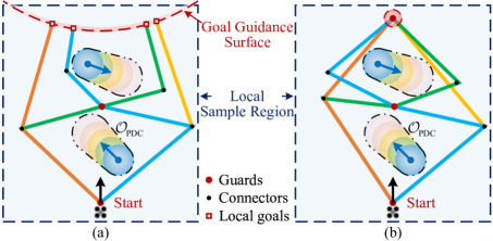
Figure 6: Illustration of Goal Guidance Surface (GCS). (a) The topological paths terminate at relaxed local goals on the GCS to improve optimality. (b) Near the global goal, the GCS degenerates to a single point.

In summary, based on these enhancements, the proposed DEV-PRM is outlined in Algorithm 2. Given current start position ${\bf p}_{s}$, the global goal ${\bf p}_{\text{goal}}$, and $\{\mathcal{O}_{\text{PDC}}\}$ of dynamic obstacles, DEV-PRM outputs the topological path set ${\bf\Pi}$. At first, based on the maximum velocity $v_{\text{max}}$ and the planning horizon $T_{h}$, $r_{\text{des}}$ is estimated to construct the $\mathcal{S}_{\text{GGS}}$ for guiding local planning. Then, the obstacle-aware samples $\mathcal{P}_{\text{PDC}}$ are precomputed to inform fast initialization of the roadmap $\mathcal{G}$. Next, $\mathcal{G}$ is further constructed by random sampling within given computation constraints, i.e., sample time $T_{\text{max}}$ and sample numbers $N_{\text{max}}$. Finally, we employ the beam search method [41] (limited width-first search) to efficiently extract a diverse set of candidate path sets ${\bf\Pi}_{\text{raw}}$. These candidate paths are then sorted by path length and filtered according to their homotopy classes to produce the final output ${\bf\Pi}$.

Input: ${\bf p}_{s}$, ${\bf p}_{g}$, $\{\mathcal{O}_{\text{PDC}}\}$

Output: TopoPathSet ${\bf\Pi}=\{{\Pi}_{1},\ldots,{\Pi}_{n}\}$

1 $r_{\text{des}}\leftarrow\|{\bf p}_{s}-{\bf p}_{g}\|-T_{h}v_{\text{max}}$ ;

2 Create the $\mathcal{S}_{\text{GGS}}$(${\bf p}_{g}$, $r_{\text{des}}$) ;

3 $\mathcal{G}$.AddGuard(${\bf p}_{s}$), $\mathcal{G}$.AddGuard($\mathcal{S}_{\text{GGS}}$);

4 for each $\mathcal{O}_{\text{PDC}}$ do $\mathcal{P}_{\text{PDC}}\leftarrow\mathcal{P}_{\text{PDC}}\cap\{{\bf p}\in\partial\mathcal{O}_{\text{PDC}}\}$;

5 ConstructRoadMap($\mathcal{G}$, $\mathcal{P}_{\text{PDC}}$);

6 ConstructRoadMapRandomly($\mathcal{G}$, $t_{\text{max}}$, $N_{\text{max}}$);

7 ${\bf\Pi}_{\text{raw}}\leftarrow$ BeamSearch($\mathcal{G}$);

${\bf\Pi}\leftarrow$ TopoPathSelect(${\bf\Pi}_{\text{raw}}$);

// by UVD

8 return ${\bf\Pi}$ ;

Algorithm 2 DEV-PRM Algorithm

III-D Spatial-temporal Trajectory Optimization

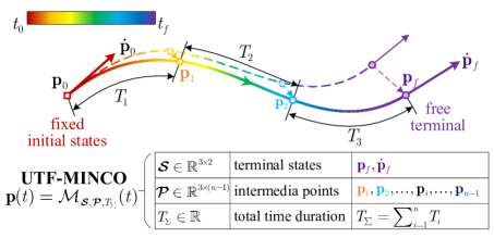
Figure 7: Illustration of UTF-MINCO trajectory parameterization.

For fast and efficient parallel trajectory computation, we adopt a Uniform Terminal-Free MINCO (UTF-MINCO) to parameterize the local trajectory optimization problem, which enables greater flexibility in local terminal adaptation under dynamic obstacles. As illustrated in Fig. 7, the UTF-MINCO parameterizes the trajectory $\mathbf{p}(t)$ by $n$ segments of piecewise continuous $m$-order polynomials ($m=5$ in this paper) as

$$\mathbf{p}(t)=\mathbf{C}_{i}^{\top}\cdot\mathbf{b}(t-t_{i-1}),t\in[t_{i-1},t_{i}],i=1,\ldots,n$$ (3)

where $\mathbf{C}_{i}\in\mathbb{R}^{(m+1)\times 3}$ is the coefficient matrix. $\mathbf{b}(t)=[1,t,t^{2},\ldots,t^{m}]^{\top}\in\mathbb{R}^{m+1}$ denotes the polynomial basis. $t_{i}$ represents the intermediate time stamp for two adjacent segments, with the corresponding joint position $\mathbf{p}(t_{i})=\mathbf{p}_{i}$. In particular, the initial and final time stamps are denoted as $t_{0}$ and $t_{f}$, respectively, whose positions are $\mathbf{p}_{0}$ and $\mathbf{p}_{f}$. To ensure the uniform distribution of control points, the time duration of each segment is set as $T_{i}=t_{i}-t_{i-1}=(t_{f}-t_{0})/n$.

Then, the UTF-MINCO formulates (3) as following compact form

$$\mathbf{p}(t)=\mathcal{M}_{\mathbfcal{S},\mathbfcal{P},T_{\Sigma}}(t)$$ (4)

in which, $\mathbfcal{S}=[\mathbf{p}_{f},\dot{\mathbf{p}}_{f}]\in\mathbb{R}^{3\times 2}$ represents the free terminal states. $\mathbfcal{P}=[\mathbf{p}_{1},\mathbf{p}_{2},\ldots,\mathbf{p}_{i},\ldots,\mathbf{p}_{n-1}]\in\mathbb{R}^{3\times(n-1)}$ denotes the intermediate control points. And $T_{\Sigma}=\sum_{i=1}^{n}T_{i}$ is the total flight duration. In (4), $\mathcal{M}$ is a linear-time and space complex mapping from $\mathbfcal{S}$, $\mathbfcal{P}$ and $T_{\Sigma}$ to the polynomials as

$$\mathbfcal{C}=\mathbfcal{A}^{-1}(T_{\Sigma})\cdot\mathbfcal{D}(\mathbfcal{S},\mathbfcal{P})$$ (5)

where $\mathbfcal{C}={\rm col}\{\mathbf{C}_{1},\ldots,\mathbf{C}_{n}\}\in\mathbb{R}^{6n\times 3}$ represents the column-wise arrangement of coefficients. $\mathbfcal{A}$ is a non-singular band matrix, and $\mathbfcal{D}$ is the boundary matrix (for details, see [10]).

Based on the UTF-MINCO, we formulate the local trajectory optimization as the following unconstrained optimization

$$\underset{\scriptscriptstyle\mathbfcal{S},\mathbfcal{P},T_{\Sigma}}{\textbf{min}}\enskip\mathcal{J}=\mathcal{H}(\mathbfcal{S},T_{\Sigma})+\mathcal{I}[\mathbfcal{C}(\mathbfcal{S},\mathbfcal{P},T_{\Sigma}),T_{\Sigma}]$$ (6)

in which, $\mathcal{H}$ denotes the cost term that directly acts on the UTF-MINCO control parameters $\mathbfcal{S}$ and $T_{\Sigma}$, while the term $\mathcal{I}$ represents the integral cost defined among the polynomials. The analytical gradients of (6) can be derived to facilitate efficient iteration in the optimization process, as follows

$$\frac{\partial\mathcal{J}}{\partial{\mathbfcal{S}}}=\frac{\partial\mathcal{H}}{\partial{\mathbfcal{S}}}+\frac{\partial\mathcal{I}}{\partial{\mathbfcal{S}}},\frac{\partial\mathcal{J}}{\partial{\mathbfcal{P}}}=\frac{\partial\mathcal{I}}{\partial{\mathbfcal{P}}},\frac{\partial\mathcal{J}}{\partial{T_{\Sigma}}}=\frac{\partial\mathcal{H}}{\partial T_{\Sigma}}+\frac{1}{n}\sum_{i=1}^{n}\frac{\partial\mathcal{I}}{\partial{T_{i}}}$$ (7)

where $\frac{\partial\mathcal{I}}{\partial{\mathbfcal{P}}}$ and $\frac{\partial\mathcal{I}}{\partial{T_{i}}}$ follow the spatial-temporal gradient conversion of the original MINCO [10]. Differently, in (7), the term $\frac{1}{n}\sum_{i=1}^{n}\frac{\partial\mathcal{I}}{\partial{T_{i}}}$ arises due to the uniform discretization of the total time $T_{\Sigma}$. On the other hand, $\frac{\partial\mathcal{I}}{\partial\mathbfcal{S}}$, i.e., the gradient with respect to the terminal states $\mathbfcal{S}$, is derived as

$$\frac{\partial\mathcal{I}}{\partial\mathbfcal{S}}=\begin{bmatrix}\mathbfcal{G}_{[6n-2,:]}\\ \mathbfcal{G}_{[6n-1,:]}\end{bmatrix}^{\top},\quad\mathbfcal{G}=\mathbfcal{A}^{-\top}\cdot\frac{\partial\mathcal{I}}{\partial{\mathbfcal C}}\in\mathbb{R}^{6n\times 3}$$ (8)

where the notation $\mathbfcal{G}_{[i,:]}$ denotes the $i^{\text{th}}$ row of $\mathbfcal{G}$.

In this paper, the objective $\mathcal{J}$ in (6) is designed as

$$\mathcal{J}=[\mathcal{H}_{t},\mathcal{H}_{s},\mathcal{I}_{o},\mathcal{I}_{d},\mathcal{I}_{e}]\cdot{\boldsymbol{\lambda}}$$ (9)

in which, ${\boldsymbol{\lambda}}\in\mathbb{R}^{5}$ is the weight vector, and the corresponding cost terms $\mathcal{H}_{t}$, $\mathcal{H}_{s}$, $\mathcal{I}_{o}$, $\mathcal{I}_{d}$, $\mathcal{I}_{e}$ are detailed as follows.

III-D1 Flight duration cost $\mathcal{H}_{t}$

The cost $\mathcal{H}_{t}=T_{\Sigma}$ is introduced to minimize the flight time for fast traversal. The gradient are given by $\frac{\partial\mathcal{H}_{t}}{\partial T_{\Sigma}}=1$.

III-D2 Heuristic terminal guidance cost $\mathcal{H}_{s}$

To guide the drone to approach the given global goal position $\mathbf{p}_{g}\in\mathbb{R}^{3}$, the cost $\mathcal{H}_{s}$ is designed as following heuristical form

$$\begin{split}&\mathcal{H}_{s}=\|\mathbf{p}_{f}-\mathbf{p}_{g}\|_{{\bf K}_{f}^{p}}^{2}+\alpha\|\dot{\mathbf{p}}_{f}\|_{{\bf K}_{f}^{\dot{p}}}^{2}\\ &\frac{\partial\mathcal{H}_{s}}{\partial{\mathbf{p}}_{f}}=2{\bf K}_{f}^{p}\cdot(\mathbf{p}_{f}-\mathbf{p}_{g}),\quad\frac{\partial\mathcal{H}_{s}}{\partial\dot{\mathbf{p}}_{f}}=2\alpha{\bf K}_{f}^{\dot{p}}\cdot\dot{\mathbf{p}}_{f}\end{split}$$ (10)

in which, $\|\mathbf{x}\|_{\mathbf{K}}^{2}=\mathbf{x}^{\top}\mathbf{K}\mathbf{x}$ represents the squared weighted norm. $\mathbf{K}_{f}^{p},\mathbf{K}_{f}^{\dot{p}}\in\mathbb{R}^{3\times 3}$ are the positive definite weighting matrices for the terminal position and velocity errors, respectively. Here, $\alpha$ serves as an adjustment coefficient. In practice, it is set to zero when the drone is far from the goal. As the drone approaches the global goal position, $\alpha$ increases gradually to reduce the terminal velocity error as follows

$${\alpha}=\begin{cases}1-\frac{\|{\bf p}_{0}-{\bf p}_{g}\|}{d_{\varepsilon}},&{\text{if}}\ {\|{\bf p}_{0}-{\bf p}_{g}\|\leq d_{\varepsilon}},\\ {0,}&{\text{otherwise.}}\end{cases}$$ (11)

where $d_{\varepsilon}$ is a threshold distance.

As for the integral functional objective $\mathcal{I}$, we utilize the trapezoidal method to approximate its value among the whole polynomials as the sum of the integrand function $\mathcal{L}(\mathbf{C}_{i},t)$ evaluated at discrete sample time $t_{k}$, given by

$$\mathcal{I}[\mathcal{L}]=\sum_{i=1}^{n}\mathcal{I}_{i}=\sum_{i=1}^{n}\sum_{k=0}^{\kappa}\omega_{k}\cdot\frac{T_{i}}{\kappa}\cdot\mathcal{L}(\mathbf{C}_{i},t_{k})$$ (12)

in which, $\mathcal{I}_{i}$ is the objective value for the $i^{\text{th}}$ segment. $\kappa$ is the number of sampling intervals. $t_{k}=k\frac{T_{i}}{\kappa}+\sum_{j=1}^{i-1}T_{j}$ is the discrete sample time stamp. $\omega_{k}$ denotes the trapezoidal coefficient, taking the value as $\frac{1}{2}$ for $k=0$ or $k=\kappa$, and $1$ otherwise. The partial derivatives of $\mathcal{I}_{i}$ are given by

$$\frac{\partial\mathcal{I}_{i}}{\partial\mathbf{C}_{i}}=\sum_{k=0}^{\kappa}\omega_{k}\cdot\frac{T_{i}}{\kappa}\cdot\frac{\partial\mathcal{L}}{\partial\mathbf{C}_{i}}$$ (13a)

$$\frac{\partial\mathcal{I}_{i}}{\partial T_{i}}=\frac{\mathcal{I}_{i}}{T_{i}}+\sum_{k=0}^{\kappa}\omega_{k}\cdot\frac{T_{i}}{\kappa}\cdot\frac{k}{\kappa}\cdot\frac{\partial\mathcal{L}}{\partial t}$$ (13b)

$$\frac{\partial\mathcal{I}_{i}}{\partial T_{j}}=\sum_{k=0}^{\kappa}\omega_{k}\cdot\frac{T_{i}}{\kappa}\cdot\frac{\partial\mathcal{L}}{\partial t},\;j=1,2,\ldots,i-1$$ (13c)

Notice that, the term (13c) does not appear in the original MINCO formulation [10]. It arises due to the time coupling among polynomial segments, e.g., for dynamic obstacle avoidance $\mathcal{I}_{o}$, the time alignment between moving obstacles and the ego must be considered, introducing the additional coupling term (13c).

The integral costs $\mathcal{I}_{o}$, $\mathcal{I}_{d}$ and $\mathcal{I}_{e}$ are detailed as follows.

III-D3 Obstacle avoidance penalty $\mathcal{I}_{o}$

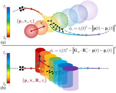
Figure 8: Illustrations of dynamic distance field (DDF) for obstacle avoidance. (a) DDF for a dynamic sphere obstacle. (b) DDF for a dynamic cylinder obstacle, where $\mathbf{R}_{o}$ denotes its rotation matrix, and $\mathbf{G}_{xy}=\mathrm{diag}(1,1,0)$ is the projection matrix onto the XY-plane.

In order to achieve both spatial and temporal obstacle avoidance, as shown in Fig.8, we introduce the Dynamic Distance Field (DDF) of dynamic obstacles. Based on the observed current position $\mathbf{p}_{o}$ and velocity ${\bf v}_{o}$ at initial time stamp $t_{0}$, the future position of a dynamic obstacle $\mathcal{O}$ can be predicted as ${\mathbf{p}_{o}}(t)$. The uncertainty of its motion is reflected through a time-varying increasing avoidance radius $r_{o}(t)=r_{o}+r_{\rm safe}+\mu_{o}\cdot(t-t_{0})$, where $r_{o}$ represents the intrinsic size of the obstacle, $r_{\rm safe}$ is the additional safety margin, and $\mu_{o}$ denotes the uncertainty provided by the dynamic obstacle estimator.

Fig.8 illustrates the DDF for spherical and cylindrical obstacles as examples. $\phi_{o}$ is the signed squared distance between the ego trajectory with respect to the predicted obstacle surface. $\phi_{o}$ becomes positive when the trajectory violates the inflated avoidance region. Thus, based on the DDF, the following penalty is introduced to ensure spatial-temporal avoidance as

$$\mathcal{L}_{o}=\sum_{\mathcal{O}}f_{\text{max}}\{\phi_{o}[\mathbf{p}(t),\mathbf{p}_{o}(t),r_{o}(t)]\}$$ (14)

where $f_{\text{max}}(x)$ is a smooth approximation of $\text{max}(x,0)$ as described in [42]. The derivatives of $\phi_{o}$ are given as follows

$$\begin{split}\frac{\partial\phi_{o}}{\partial\mathbf{C}_{i}}&=\mathbf{b}\cdot\left(\frac{\partial\phi_{o}}{\partial{\mathbf{p}}}\right)^{\top}\\ \frac{\partial\phi_{o}}{\partial t}&=\underbrace{\left(\frac{\partial\phi_{o}}{\partial{\mathbf{p}}}\right)^{\top}\cdot\dot{{\mathbf{p}}}}_{\text{(a) derivative of ego}}+\underbrace{\left(\frac{\partial\phi_{o}}{\partial{\mathbf{p}}_{o}}\right)^{\top}\cdot\dot{{\mathbf{p}}}_{o}+\frac{\partial\phi_{o}}{\partial r_{o}}\cdot\dot{r}_{o}}_{\text{(b) derivative of dynamic obstacles}}\end{split}$$ (15)

Note that, the time derivative $\frac{\partial\phi_{o}}{\partial t}$ contains two main terms, the derivative of the ego trajectory (15a), and the additional derivative of the dynamic obstacle (15b). As described in (13), the term (15a) only affects $\frac{\partial\mathcal{I}_{i}}{\partial T_{i}}$ of $i^{\text{th}}$ trajectory segment. In contrast, the remaining (15b) arises from the alignment between the ego trajectory and the dynamic obstacle, thereby introducing additional temporal coupling that contributes to both $\frac{\partial\mathcal{I}_{i}}{\partial T_{i}}$ and $\frac{\partial\mathcal{I}_{i}}{\partial T_{j}}$ for $j=1,2,\ldots,i-1$.

III-D4 Dynamic feasibility cost $\mathcal{I}_{d}$

The flight speed and acceleration of a drone are constrained by its physical capabilities. Therefore, $\mathcal{I}_{d}$ is designed by penalizing $\mathcal{L}_{d}^{v}=f_{\max}(\phi_{v})$ and $\mathcal{L}_{d}^{a}=f_{\max}(\phi_{a})$ with

$$\phi_{v}=\frac{\mathbf{v}^{\top}\mathbf{v}}{v_{\max}^{2}}-1,\quad\phi_{a}=\frac{\mathbf{a}^{\top}\mathbf{a}}{a_{\max}^{2}}-1$$ (16)

in which, $v_{\max}$ and $a_{\max}$ denote the maximum speed and acceleration, respectively. The gradients of (16) are given by

$$\begin{split}\frac{\partial\phi_{v}}{\partial\mathbf{C}_{i}}&=\frac{2\dot{\mathbf{b}}\mathbf{v}^{\top}}{v_{\max}^{2}},\quad\frac{\partial\phi_{v}}{\partial t}=\frac{2\mathbf{a}^{\top}\mathbf{v}}{v_{\max}^{2}}\\ \frac{\partial\phi_{a}}{\partial\mathbf{C}_{i}}&=\frac{2\ddot{\mathbf{b}}\mathbf{a}^{\top}}{a_{\max}^{2}},\quad\frac{\partial\phi_{a}}{\partial t}=\frac{2\mathbf{j}^{\top}\mathbf{a}}{a_{\max}^{2}}\end{split}$$ (17)

where $\mathbf{j}=\dddot{\mathbf{p}}\in\mathbb{R}^{3}$ denotes the jerk vector.

III-D5 Jerk minimization cost $\mathcal{I}_{e}$

$\mathcal{I}_{e}$ penalizes the $3^{\rm rd}$ derivative of the trajectory, i.e., the jerk, to promote smoother motions and reduce the control efforts. The corresponding integrand function $\mathcal{L}_{e}$ and its gradients are given by

$$\mathcal{L}_{e}=\mathbf{j}^{\top}\mathbf{j},\quad\frac{\partial\mathcal{L}_{e}}{\partial\mathbf{C}_{i}}=2\dddot{\mathbf{b}}^{\top}\mathbf{j},\quad\frac{\partial\mathcal{L}_{e}}{\partial t}=2\mathbf{s}^{\top}\mathbf{j}$$ (18)

where $\mathbf{s}=\ddddot{\mathbf{p}}\in\mathbb{R}^{3}$ denotes the snap vector.

In summary, with the above problem formulation, the spatial-temporal trajectory optimization is transcribed as a lightweight unconstrained nonlinear programming as shown in (6). The flight trajectories are compactly parameterized by the free terminal states $\mathbfcal{S}$, the intermediate control points $\mathbfcal{P}$ and time duration $T_{\Sigma}$, resulting in the lower-dimensional characteristic of the problem. Owing to the analytical gradients, it requires only a single function evaluation per gradient iteration, resulting in linear time and space complexity. Therefore, using gradient-based solvers such as L-BFGS [43], (6) enables efficient parallel computation of multiple trajectories with different spatial-temporal topologies to explore diverse solutions in real time.

IV Simulation Experiments and Results

This section presents several simulation experiments to validate the performance of the proposed method. The software of TRUST-Planner is implemented by C++ under ROS 2 (Humble) [44] environment on a desktop computer with a 2.2 GHz Intel Core i9-13980HX CPU and 16 GB RAM. The simulation drone follows the planned trajectories by a nonlinear controller [35] with constraints $v_{\max}=2\,\mathrm{m/s}$ and $a_{\max}=3\,\mathrm{m/s^{2}}$. The planner does not have access to the precise future motion of dynamic obstacles, but only the current position and velocity to estimate by utilizing Extended Kalman Filter (EKF) [45]. Sec.IV-A and IV-B presents a module-wise evaluation, including comparative studies of the proposed DEV-PRM and UTF-MINCO against several competitors, respectively. Sec.IV-C analyzes the spatial-temporal topological trajectory planning results in a random dynamic environment. And Sec.IV-D compares the overall performance of TRUST-Planner with several hierarchical planning frameworks to demonstrate the advantages of the proposed method. The details are as follows.

IV-A Topological Path Planning

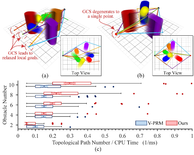
Figure 9: Topological path planning results of DEV-PRM in random dynamic environments. (a) $\mathcal{S}_{\text{GGS}}$ with ${\bf p}_{g}=[13,0,5]^{\top}\,\mathrm{m}$ and $r_{\text{des}}=5\,\mathrm{m}$. (b) $\mathcal{S}_{\text{GGS}}$ with ${\bf p}_{g}=[8,0,5]^{\top}\,\mathrm{m}$ and $r_{\text{des}}=0\,\mathrm{m}$. (c) Comparison on the numbers of found topological paths per unit time.

We first compare the performance of the proposed DEV-PRM with the state-of-the-art V-PRM [8] to demonstrate its effectiveness for topological path planning in dynamic environments. The test scenarios are constructed within a $4\times 4\times 2\,\mathrm{m^{3}}$ area containing randomly generated dynamic cylindrical and spherical obstacles. The prediction horizon for dynamic obstacles is set to $T_{h}=4\,\mathrm{s}$, and both methods are limited to a maximum computation time of $t_{\rm max}=20\,\mathrm{ms}$. As shown in Fig.9, DEV-PRM successfully generates homotopy-distinct reference paths that avoid dynamic obstacles within the prediction horizon. In Fig.9(a) and (b), when the GGS is positioned far from the goal ${\bf p}_{g}$, DEV-PRM produces topological paths with relaxed local endpoints. As the GGS is close to the goal, it shrinks to a single point, causing DEV-PRM to degenerate into the original behavior of V-PRM with fixed local endpoints. Fig.9(c) further provides a quantitative comparison of the computational efficiency of DEV-PRM and V-PRM under varying numbers of random obstacles, in which the $x$-axis represents the ratio of found homotopy-distinct paths to the roadmap construction time. Across all tests, benefiting from the obstacle-aware sampling strategy, DEV-PRM consistently discovers more topological paths per unit time than V-PRM. Specifically, with 10 random dynamic obstacles, DEV-PRM achieves an average exploration efficiency of 0.338 (found topological paths/CPU time), compared to 0.186 for V-PRM, representing an 81.9% improvement. These results validate the superior efficiency and topological diversity of DEV-PRM in dynamic environments.

IV-B Trajectory Optimization

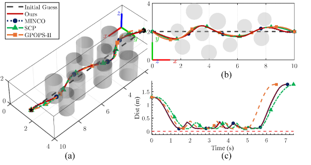
Figure 10: Companions of trajectory optimization methods in a static scenario. (a) Trajectories. (b) Top view of the trajectories. (c) Distance to the obstacles.

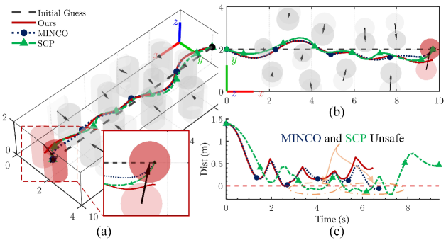
Figure 11: Companions of trajectory optimization methods in a dynamic scenario, in which the red obstacle is blocking the goal position. (a) Trajectories. (b) Top view of the trajectories. (c) Distance to the obstacles.

TABLE I: Comparisons of Different Trajectory Optimization Methods

Method	Static CASE			Dynamic CASE
	CPU Time	Duration		CPU Time	Duration
Ours	8.98	7.08		9.71	6.47
MINCO [10]	7.77	7.09		8.52	6.72
SCP [9]	301.7	7.40		511.4	9.72
GPOPS-II [11]	8127.3	6.51		Failed	Failed

The performance of the proposed UTF-MINCO is compared with several trajectory optimization methods, including the original MINCO[10], SCP [9] solved by ECOS [46], and GPOPS-II [11]. As illustrated in Fig.10–11, two test scenarios are designed to evaluate these methods. In the simple static scenario, all methods successfully generate feasible trajectories to avoid the obstacles while reaching the goal position. However, the competitors struggle to adapt to the more challenging dynamic scenario, where the moving obstacles gradually block the trajectories and the terminal states (red obstacle). As a result, the trajectories generated by these methods collide with dynamic obstacles. In contrast, owing to the designed DDF and relaxed terminal formulation, our method, UTF-MINCO continuously maintains a safe distance from dynamic obstacles and successfully avoids all the dynamic obstacles. Notably, GPOPS-II failed to produce a feasible trajectory in the dynamic scenario within a reasonable CPU time. The CPU Time (50 times average in milliseconds) and trajectory duration (in second) are summarized in Table I. In terms of optimality, all the competitors are with similar flight duration. However, our method achieves millisecond-level computation time, which is much faster than SCP and GPOPS-II. Note that our method takes slightly more time than MINCO due to the additional optimization variables introduced by the relaxed terminal, but this overhead brings the improvement of the obstacle avoidance flexibility in dynamic environments. Overall, these results demonstrate that our method provides greater flexibility, safety, and computational efficiency in dynamic environments, enabling subsequent parallel optimization of multiple topological trajectories in real-time.

IV-C Spatial-temporal Topological Trajectory Planning

TABLE II: Comparisons of Spatial-temporal Topological Trajectories

Idx	$\mathcal{H}_{t}$	$\mathcal{H}_{s}$	$\mathcal{I}_{e}$	$\mathcal{J}$	CPU Time (ms)
$\tau_{0}$	4.38	5.05	50.52	7.41	10.93
$\tau_{1}$	4.58	5.04	53.87	7.64	7.031
$\tau_{2}$	4.87	5.05	32.85	7.72	3.37
$\tau_{3}$	4.87	5.04	82.59	8.22	7.53
$\tau_{4}$	5.65	5.05	108.98	9.27	5.51

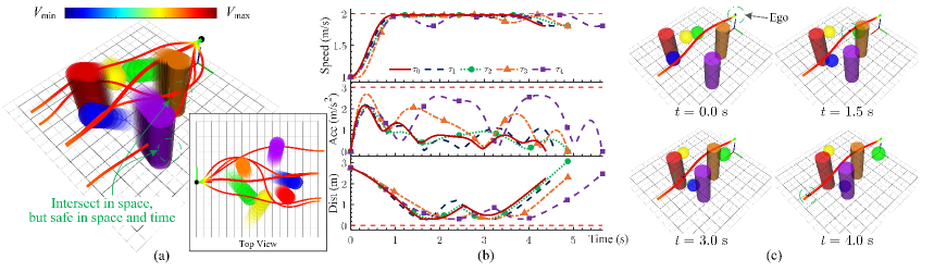
Figure 12: Spatial-temporal topological trajectory planning results. (a) Spatial-temporal topological trajectories. (b) The speed profiles, acceleration and minimal distance to the obstacles. (c) Following process of the optimal trajectory $\tau_{0}$.

This subsection analyzes the spatial-temporal topological trajectory planning results of TRUST-Planner. The planning scenario is similar to Fig.9(a) in Sec.IV-A, containing 6 random dynamic obstacles. By leveraging the proposed DEV-PRM as an initial guide, TRUST-Planner generates multiple distinct spatial-temporal topological trajectories. The initial speed is ${\bf v}_{0}=[1,0,0]^{\top}\,\mathrm{m/s}$. The topological trajectories are sorted by total cost $\mathcal{J}$, with weights $\lambda_{t}=1$, $\lambda_{s}=1/v_{\rm max}$ and $\lambda_{e}=0.01$. The planning results are shown in Fig.12. As shown in Fig.12(a), five homotopy-distinct trajectories are generated, denoted as $\tau_{0}$–$\tau_{4}$. Notice that, although some trajectories interests with the PDCs of dynamic obstacles in space, they are all collision-free in the spatial-temporal domain. In Fig.12(b), the flight speed, acceleration, and minimal distance to the obstacles are all within the corresponding constraints. The local terminal speeds of the trajectories are consistently maintained at approximate 0.9$v_{\rm max}$, which is intended to ensure a relatively high initial speed that facilitates a rapid convergence toward the global goal in subsequent planning horizons. The quantitative comparisons of these trajectories are provided in Table II, including the flight duration $\mathcal{H}_{t}$, heuristic terminal cost $\mathcal{H}_{s}$, and jerk cost $\mathcal{I}_{e}$. Among them, the trajectory $\tau_{0}$ achieves the lowest weighted cost $\mathcal{J}$, and thus is selected as the optimal main branch for the ego drone to follow and execute. Fig.12(c) illustrates the following process, where the ego drone rapidly crosses dynamic obstacles and continues its forward flight. Notice that, owing to the high efficiency of the low-level trajectory optimization, the proposed method can rapidly compute all these trajectories in parallel, with a maximum CPU time of 10.93 ms, fully satisfying the real-time requirements of practical applications. Moreover, all generated trajectories are feasible and collision-free, providing a set of safe alternatives for emergency obstacle avoidance, which further enhances the robustness and flexibility of the proposed planner in dynamic environments.

IV-D Comparative Studies with Baseline Methods

In this subsection, the overall performance of TRUST-Planner is compared with several baseline methods to further demonstrate the advantages of the proposed approach. To this end, we design a challenging random obstacle map with dimensions of $50\times 15\times 5\,\mathrm{m}^{3}$, densely filled with static obstacles represented by point clouds (utilizing Euclidean Signed Distance Field [40] for static collision avoidance), as well as 100 randomly generated dynamic cylinder obstacles. For all baseline methods, the trajectory optimization backend employs our UTF-MINCO parameterization combined with the proposed dynamic distance field (DDF) for obstacle avoidance. The primary distinction among the competitors lies in the hierarchical guidance strategies, summarized as follows:

• Baseline 1: No hierarchical guidance. Use a straight line towards the goal as the trajectory initial guess.

• Baseline 2: Referring to [9], use the shortest geometric path computed by the Sparse A* as the initial guess for trajectory optimization. It can be regarded as a single topological guidance method.

• Baseline 3: Referring to Fast-Planner [8], employ the proposed DEV-PRM to generate multiple topological guidance paths for parallel trajectory optimization, and then simply select the optimal trajectory for execution. However, it does not maintain or manage historical topological information during replanning, resulting in the loss of previously explored topological branches.

• Ours: The proposed TRUST-Planner integrates topological guidance with multi-branch management, enabling robust and efficient spatial-temporal trajectory planning.

For each competitor, 100 times Monte-Carlo simulations are conducted to statistically evaluate their performance in terms of safe arrival success rate, average computation time, and arrival time (optimality). The results are illustrated in Fig.13–15.

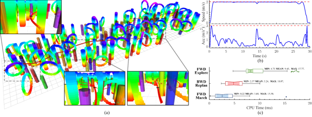
Figure 13: Trajectory planning results of the proposed TRUST-Planner in the tested obstacle environment. (a) Flight processes, in which the enlarged sub-figures highlight the local multiple-branch topological trajectories. (b) The speed profiles and acceleration. (c) CPU time statistics of the incremental planning process.

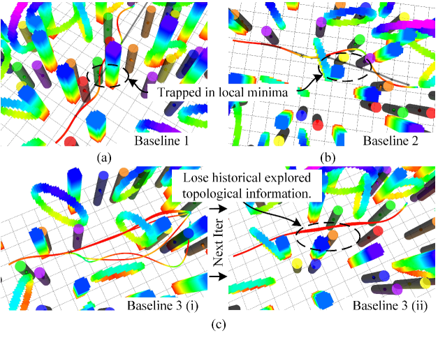
Figure 14: Flight processes of the baseline competitors. (a) and (b) Local minima phenomenon of Baseline 1 and Baseline 2, respectively, leading to collisions. (c) Baseline 3, without topological management, loses previously explored information in replanning, resulting in suboptimal and eventual collision.

Fig.13 firstly shows a representative planning result of the proposed TRUST-Planner in the complex obstacle environment. Leveraging multi-branch topological trajectory guidance, our method enables the ego drone to successfully avoid both static and dynamic obstacles and reach the goal position quickly. Fig.13(b) shows that the drone maintains near-maximum speed while traversing the obstacle-rich area, completing the flight in 29.4 s. Fig.13(c) counts the computation time statistics of the incremental planning process. Owing to incremental topological management, the replanning of the existing main branch (FWD March) and sub-branches (BWD Replan) is relatively fast, with average computation times of 3.40 ms and 5.24 ms, respectively. The exploration of new topological trajectories (FWD Explore) takes slightly longer, as it requires a DEV-PRM topological path planning step; however, the average computation time of each trajectory still remains low at 9.45 ms. Overall, the parallel computation time of the proposed TRUST-Planner is consistently around the order of 10 ms.

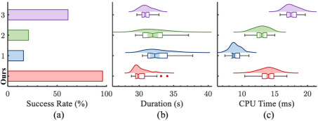
Figure 15: Statistical comparisons of baseline competitors. (a) Success rate of safe arrival. (b) Arrival flight duration (optimality). (c) Average CPU time.

As a contrast, Fig.14 illustrates typical failure cases of the baseline competitors. Baseline 1, which relies solely on a straight-line initial guess, is highly prone to becoming trapped in local minima and unable to escape, leading to high collision rates. As for Baseline 2, although guided by the shortest path, it still suffers from the structural inconsistency between geometric paths and spatio-temporal trajectories. As a result, the derived trajectory may still be trapped in local minima and collide with obstacles. Baseline 3 employs a multi-topology guidance strategy, enabling the planner to select the alternate trajectory to jump out of local optimum for safety and optimality improvement. However, due to the lack of effective topological branch management, it may lose historical topological information during replanning. Thus, the randomized topological path searching may not be effective to discover sufficiently diverse topological guidance paths in complex environment, leading to suboptimal and eventual collision.

Fig.15 presents the statistical comparisons of all methods over 100 Monte Carlo simulations. Notice that, the planners can not access the precise future motion of dynamic obstacles and rely on estimations for collision avoidance. Therefore, in such challenging scenarios, the baseline methods exhibit low success rates of safe arrival, while the proposed method achieves a much higher success rate of 96%. In terms of optimality, our method leverages optimal selection of spatial-temporal topological to maintain high-speed traversal in the obstacle area, achieving an average flight duration of 29.4 s, which is faster than all baseline methods. As for computational efficiency, since Baseline 2, 3 and ours require additional frontend path planning, they take longer CPU time for trajectory generation than Baseline 1. However, owing to the incremental multi-branches topological management and parallel computation strategy, our method enable rapid trajectory generation at the 10 ms level, and reduces the average planning time of single trajectory by 19.72% compared to Baseline 3.

In summary, the proposed TRUST-Planner demonstrates superior performance in terms of robustness, optimality, and computational efficiency.

V Real-world Experiments

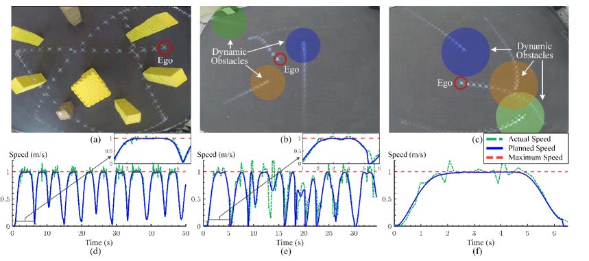
Figure 16: Real-world experiment results. (a) Random flight in a static environment. (b) Random flight in a dynamic environment. (c) Penetration flight in a dynamic environment. (d)-(f) The flight speed profiles of the ego in the three scenarios.

In this section, the real-world experiments are performed to further validate the feasibility and engineering practicality of TRUST-Planner. The flight platform is based on the Crazyfile 2.1 nano-scale drone, integrated with an OptiTrack motion capture system for high-precision indoor localization. Our method is implemented on the ground station as a real-time planning terminal, using Crazyswarm 2 [47] software to communicate with the drones via radio link. The dynamic constraints are set as $v_{\max}=1\,\mathrm{m/s}$, $a_{\max}=3\,\mathrm{m/s^{2}}$.

Three different scenarios are designed as follows. Notice that, in all cases, the ego drone can only obtain the position of obstacles from the motion capture system, and predicts their future motion based on historical and current information to spatial-temporal avoidance.

1. Random flight in a static environment. The ego drone is navigated to the random published goals, while avoiding static obstacles in a $4\times 4\times 2\,\mathrm{m^{3}}$ area.

2. Random flight in a dynamic environment. The ego drone is assigned to the random published goals, while avoiding three patrol drones (as dynamic obstacles) that move along predefined trajectories.

3. Penetration flight in a dynamic environment. Three drones act as the interceptors using the classic proportional guidance law [48] to intercept the ego, who is required to penetrate through them quickly.

The results of flight experiments are shown in Fig.16. During the flight, the ego drone continuously replans its local trajectories to avoid obstacles while heading towards randomly assigned global goals. Especially for the last two scenarios, since the ego drone does not know the precise future motion of the dynamic obstacles, autonomous flights in such unknown environments are quite challenging. However, the proposed TRUST-Planner can still realize millisecond-level trajectory replanning to avoid unknown maneuvers of obstacles. Fig.16(d)-(f) further show the part of speed profiles of the ego. In these scenarios, the ego tends to quickly traverse the obstacle area at maximum speed, demonstrating the optimality of the proposed trajectory planning approach. The actual speed (green dotted lines) accurately follows the planned speed profiles (blue solid line), which also shows the feasibility of the planned trajectories.

In summary, the real-world experiments illustrate the excellent computational efficiency and applicability of the proposed method.

VI Conclusions and Future Work

This paper presents a novel spatial-temporal topological trajectory planning framework, namely TRUST-Planner, for autonomous aerial vehicles operating in complex dynamic environments. Our planner integrates a dynamic enhanced visible PRM (DEV-PRM) frontend for efficient topological path exploration, a uniform terminal-free minimum control polynomial (UTF-MINCO) backend for fast and flexible trajectory optimization with predictive dynamic obstacle avoidance, and an incremental multi-branch trajectory management framework to maintain topological diversity and enable trajectory decision. Extensive simulation and real-world experiments demonstrate that TRUST-Planner achieves superior performance in terms of robustness, trajectory safety, and computational efficiency, with a 96% planning success rate and millisecond-level computation time in challenging scenarios.

Currently, TRUST-Planner relies on prediction of dynamic obstacles’ future motion for spatial-temporal dynamic obstacle avoidance. The implementation of real-world experiments uses precise 3D position and velocity data provided by a motion capture system. In future work, we aim to extend the framework to more practical scenarios by developing obstacle identification and prediction based on onboard sensing, such as point cloud data from vision or LiDAR, to further enhance the applicability and autonomy of our method.

Junzhi Li received the B.S. degree in flight vehicle design and engineering from the School of Aerospace Engineering, Beijing Institute of Technology, Beijing, China, in 2020. He is currently working toward a Ph.D. degree in aeronautical and astronautical science and technology with Beijing Institute of Technology. His research interests include trajectory optimization and control of unmanned flight vehicles.

Teng Long received the B.S. degree in flight vehicle propulsion engineering and the Ph.D. in aeronautical and astronautical science and technology from Beijing Institute of Technology, Beijing, China, in 2004 and 2009, respectively. He is currently a Professor and Dean with the School of Aerospace Engineering, Beijing Institute of Technology. His research interests include multidisciplinary design optimization theory and its applications to flight vehicle conceptual design, multi-aircraft collaborative mission planning and decision-making.

Jingliang Sun received the B.S. degree in automation from the Tianjin University of Technology, Tianjin, China, and the Ph.D. in control theory and control engineering from the Nanjing University of Aeronautics and Astronautics, Nanjing, China. He is an associate professor with the School of Aerospace Engineering, Beijing Institute of Technology. His research interests include adaptive dynamic programming, cooperative guidance and control, and cooperative mission planning in aerospace engineering.

Jianxin Zhong received the B.S. degree in flight vehicle design and engineering from Beijing Institute of Technology, Beijing, China, in 2023. He is currently working toward the M.S. degree in aeronautical and astronautical science and technology with Beijing Institute of Technology. His research interests include multi-agent path planning and cooperative task assignment of unmanned aerial vehicles.

References

- [1] J. Doornbos, K. E. Bennin, Ö. Babur, and J. Valente, “Drone Technologies: A Tertiary Systematic Literature Review on a Decade of Improvements,” IEEE Access, vol. 12, pp. 23 220–23 239, 2024.
- [2] O. De Groot, L. Ferranti, D. M. Gavrila, and J. Alonso-Mora, “Topology-driven parallel trajectory optimization in dynamic environments,” IEEE Trans. Robot., vol. 41, pp. 110–126, 2025.
- [3] L. Quan, L. Han, B. Zhou, S. Shen, and F. Gao, “Survey of UAV motion planning,” IET Cyber-Syst. Robot., vol. 2, no. 1, pp. 14–21, Mar. 2020.
- [4] J. Luo, Y. Tian, and Z. Wang, “Research on Unmanned Aerial Vehicle Path Planning,” Drones, vol. 8, no. 2, p. 51, Feb. 2024.
- [5] Y. Zhou, L. Yan, Y. Han, H. Xie, and Y. Zhao, “A Survey on the Key Technologies of UAV Motion Planning,” Drones, vol. 9, no. 3, p. 194, Mar. 2025.
- [6] G. Zhang and X. Liu, “UAV collision avoidance using mixed-integer second-order cone programming,” J. Guid., Control, Dyn., vol. 45, no. 9, pp. 1732–1738, May 2022.
- [7] Z. Zhao, S. Cheng, Y. Ding, Z. Zhou, S. Zhang, D. Xu, and Y. Zhao, “A Survey of Optimization-Based Task and Motion Planning: From Classical to Learning Approaches,” IEEE/ASME Trans. Mechatronics, pp. 1–27, 2024.
- [8] B. Zhou, F. Gao, J. Pan, and S. Shen, “Robust real-time uav replanning using guided gradient-based optimization and topological paths,” in 2020 IEEE International Conference on Robotics and Automation (ICRA), May 2020, pp. 1208–1214.
- [9] T. Long, Y. Cao, G. Xu, Z. Meng, J. Sun, and Z. Wang, “Real-time multi-quadrotor trajectory generation via distributed receding architecture and hierarchical planning in complex environments,” ISA Trans., vol. 136, pp. 715–726, May 2023.
- [10] Z. P. Wang, X. Zhou, C. Xu, and F. Gao, “Geometrically constrained trajectory optimization for multicopters,” IEEE Trans. Robot., vol. 38, no. 5, pp. 3259–3278, May 2022.
- [11] M. A. Patterson and A. V. Rao, “GPOPS-II: A MATLAB software for solving multiple-phase optimal control problems using hp-adaptive gaussian quadrature collocation methods and sparse nonlinear programming,” ACM Trans. Math. Softw., vol. 41, no. 1, pp. 1–37, Oct. 2014.
- [12] L. Lin and M. A. Goodrich, “Hierarchical heuristic search using a gaussian mixture model for UAV coverage planning,” IEEE Trans. Cybern., vol. 44, no. 12, pp. 2532–2544, Dec. 2014.
- [13] A. Bry, C. Richter, A. Bachrach, and N. Roy, “Aggressive flight of fixed-wing and quadrotor aircraft in dense indoor environments,” Int. J. Robot. Res., vol. 34, no. 7, pp. 969–1002, Mar. 2015.
- [14] S. Liu, M. Watterson, K. Mohta, K. Sun, S. Bhattacharya, C. J. Taylor, and V. Kumar, “Planning dynamically feasible trajectories for quadrotors using safe flight corridors in 3-D complex environments,” IEEE Robot. Autom. Lett., vol. 2, no. 3, pp. 1688–1695, Jul. 2017.
- [15] J. Sun, G. Xu, Z. Wang, T. Long, and J. Sun, “Safe flight corridor constrained sequential convex programming for efficient trajectory generation of fixed-wing UAVs,” Chin. J. Aeronaut., vol. 38, no. 1, p. 103174, Jan. 2025.
- [16] T. Jesus and H. Jonathan P., “MADER: Trajectory planner in multiagent and dynamic environments,” IEEE Trans. Robot., vol. 38, no. 1, pp. 463–476, Jul. 2022.
- [17] B. Zhou, F. Gao, L. Wang, C. Liu, and S. Shen, “Robust and efficient quadrotor trajectory generation for fast autonomous flight,” IEEE Robot. Autom. Lett., vol. 4, no. 4, pp. 3529–3536, Oct. 2019.
- [18] W. Ding, W. Gao, K. Wang, and S. Shen, “An efficient B-spline-based kinodynamic replanning framework for quadrotors,” IEEE Trans. Robot., vol. 35, no. 6, pp. 1287–1306, Dec. 2019.
- [19] J. Liu, M. Fu, A. Liu, W. Zhang, and B. Chen, “A homotopy invariant based on convex dissection topology and adistance optimal path planning algorithm,” IEEE Robot. Autom. Lett., vol. 8, no. 11, pp. 7695–7702, Nov. 2023.
- [20] E. H. Spanier, Algebraic topology. Springer Science & Business Media, 2012.
- [21] S. Bhattacharya, M. Likhachev, and V. Kumar, “Topological constraints in search-based robot path planning,” Auton. Robots, vol. 33, no. 3, pp. 273–290, Oct. 2012.
- [22] H. Ye, X. Zhou, Z. Wang, C. Xu, J. Chu, and F. Gao, “TGK-Planner: An efficient topology guided kinodynamic planner for autonomous quadrotors,” IEEE Robot. Autom. Lett., vol. 6, no. 2, pp. 494–501, Apr. 2021.
- [23] A. Sahin and S. Bhattacharya, “Topo-geometrically distinct path computation using neighborhood-augmented graph, and its application to path planning for a tethered robot in 3-D,” IEEE Trans. Robot., vol. 41, pp. 20–41, 2025.
- [24] W. Yu, H. Xiong, and X. Nian, “Topology-guided online trajectory planning for UAV navigation in dynamic environments,” in 2024 9th International Conference on Robotics and Automation Engineering (ICRAE). Singapore, Singapore: IEEE, Nov. 2024, pp. 28–32.
- [25] Z. Lin, K. Wu, R. Shen, X. Yu, and S. Huang, “An efficient and accurate A-star algorithm for autonomous vehicle path planning,” IEEE Trans. Veh. Technol., vol. 73, no. 6, pp. 9003–9008, May 2024.
- [26] Z. Pan, C. Zhang, Y. Xia, H. Xiong, and X. Shao, “An improved artificial potential field method for path planning and formation control of the multi-uav systems,” IEEE Trans. Circuits Syst. II, vol. 69, no. 3, pp. 1129–1133, Mar. 2022.
- [27] H. Liu, G. Wu, L. Zhou, W. Pedrycz, and P. N. Suganthan, “Tangent-based path planning for UAV in a 3-D low altitude urban environment,” IEEE Trans. Intell. Transp. Syst., vol. 24, no. 11, pp. 12 062–12 077, Nov. 2023.
- [28] T. Combelles, C. Marmonnier, L. Proffit, and L. Jouanneau, “MORRFx and its framework: Multi-objective sampling based path planning for unpredictable environments,” in 2022 7th International Conference on Mechanical Engineering and Robotics Research (ICMERR), Dec. 2022, pp. 1–6.
- [29] X.-F. Liu, Y. Fang, Z.-H. Zhan, Y.-L. Jiang, and J. Zhang, “A Cooperative Evolutionary Computation Algorithm for Dynamic Multiobjective Multi-AUV Path Planning,” IEEE Trans. Ind. Informat., vol. 20, no. 1, pp. 669–680, Jan. 2024.
- [30] E. Schmitzberger, J. Bouchet, M. Dufaut, D. Wolf, and R. Husson, “Capture of homotopy classes with probabilistic road map,” in IEEE/RSJ International Conference on Intelligent Robots and Systems, vol. 3, Sep. 2002, pp. 2317–2322 vol.3.
- [31] C. Rösmann, F. Hoffmann, and T. Bertram, “Planning of multiple robot trajectories in distinctive topologies,” in 2015 European Conference on Mobile Robots (ECMR), Sep. 2015, pp. 1–6.
- [32] P. Werner, A. Amice, T. Marcucci, D. Rus, and R. Tedrake, “Approximating robot configuration spaces with few convex sets using clique covers of visibility graphs,” in 2024 IEEE International Conference on Robotics and Automation (ICRA), May 2024, pp. 10 359–10 365.
- [33] H. Kretzschmar, M. Spies, C. Sprunk, and W. Burgard, “Socially compliant mobile robot navigation via inverse reinforcement learning,” The International Journal of Robotics Research, vol. 35, no. 11, pp. 1289–1307, Sep. 2016.
- [34] Z. Wang, L. Liu, and T. Long, “Minimum-time trajectory planning for multi-unmanned-aerial-vehicle cooperation using sequential convex programming,” J. Guid., Control, Dyn., vol. 40, no. 11, pp. 2976–2982, Sep. 2017.
- [35] D. Mellinger and V. Kumar, “Minimum snap trajectory generation and control for quadrotors,” in 2011 IEEE International Conference on Robotics and Automation. Shanghai, China: IEEE, May 2011, pp. 2520–2525.
- [36] R. Chai, A. Tsourdos, A. Savvaris, S. Chai, and Y. Xia, “Solving Constrained Trajectory Planning Problems Using Biased Particle Swarm Optimization,” IEEE Trans. Aerosp. Electron. Syst., vol. 57, no. 3, pp. 1685–1701, Jun. 2021.
- [37] J. Li, J. Sun, T. Long, and Z. Zhou, “Differential Flatness-Based Fast Trajectory Planning for Fixed-Wing Autonomous Aerial Vehicles,” IEEE Trans. Syst., Man, Cybern., pp. 1–14, 2025.
- [38] E. Tal, G. Ryou, and S. Karaman, “Aerobatic trajectory generation for a VTOL fixed-wing aircraft using differential flatness,” IEEE Trans. Robot., vol. 39, no. 6, pp. 4805–4819, Aug. 2023.
- [39] T. Jesus, L. Brett, M. Everett, and J. P. How, “FASTER: Fast and Safe Trajectory Planner for Navigation in Unknown Environments,” IEEE Trans. Robot., vol. 38, no. 2, pp. 922–938, Oct. 2022.
- [40] L. Quan, L. Yin, T. Zhang, M. Wang, R. Wang, S. Zhong, X. Zhou, Y. Cao, C. Xu, and F. Gao, “Robust and efficient trajectory planning for formation flight in dense environments,” IEEE Trans. Robot., vol. 39, no. 6, pp. 4785–4804, Dec. 2023.
- [41] A. Jaszkiewicz and R. Słowiński, “The light beam search approach: an overview of methodology applications,” Eur. J. Oper. Res., vol. 113, no. 2, pp. 300–314, Mar. 1999.
- [42] Z. Wang, C. Xu, and F. Gao, “Robust trajectory planning for spatial-temporal multi-drone coordination in large scenes,” in 2022 IEEE/RSJ International Conference on Intelligent Robots and Systems (IROS). Kyoto, Japan: IEEE, Oct. 2022, pp. 12 182–12 188.
- [43] D. C. Liu and J. Nocedal, “On the limited memory BFGS method for large scale optimization,” Math. Program., vol. 45, no. 1-3, pp. 503–528, Aug. 1989.
- [44] S. Macenski, T. Foote, B. Gerkey, C. Lalancette, and W. Woodall, “Robot operating system 2: Design, architecture, and uses in the wild,” Sci. Robot., vol. 7, no. 66, p. eabm6074, 2022.
- [45] E. A. Wan and R. Van Der Merwe, “The unscented kalman filter for nonlinear estimation,” in Proceedings of the IEEE 2000 Adaptive Systems for Signal Processing, Communications, and Control Symposium (Cat. No. 00EX373). Ieee, 2000, pp. 153–158.
- [46] A. Domahidi, E. Chu, and S. Boyd, “ECOS: An SOCP solver for embedded systems,” in 2013 European Control Conference (ECC). Zurich, Switzerland: IEEE, Jul. 2013, pp. 3071–3076.
- [47] J. A. Preiss, W. Honig, G. S. Sukhatme, and N. Ayanian, “Crazyswarm: A large nano-quadcopter swarm,” in 2017 IEEE International Conference on Robotics and Automation (ICRA), May 2017, pp. 3299–3304, software available at https://github.com/USC-ACTLab/crazyswarm.
- [48] E. Duflos, P. Penel, and P. Vanheeghe, “3D guidance law modeling,” IEEE Trans. Aerosp. Electron. Syst., vol. 35, no. 1, pp. 72–83, Jan. 1999.