Nonparametric Estimation from Correlated Copies of a Drifted 2nd-Order Process

Abstract.

This paper presents several situations leading to the observation of multiple - possibly correlated - copies of a drifted 2nd-order process, and then non-asymptotic risk bounds are established on nonparametric estimators of the drift function $b_{0}$ and its derivative. For drifted Gaussian processes with a regular enough covariance function, a sharper risk bound is established on the estimator of $b_{0}^{\prime}$, and a model selection procedure is provided with theoretical guarantees.

^†Université Paris Nanterre, CNRS, Modal’X, 92001 Nanterre, France.

Keywords: Correlated processes; Gaussian processes; Fractional Brownian motion; Functional Data; Nonparametric estimation; Drift estimation; Derivative estimation; Model selection.

1. Introduction

Let $X=(X_{t})_{t\in\mathbb{R}_{+}}$ be the process defined by

(1) $$X_{t}=b_{0}(t)+Z_{t}\textrm{ $;$ }\forall t\in\mathbb{R}_{+},$$

where $Z=(Z_{t})_{t\in\mathbb{R}_{+}}$ is a centered continuous 2nd-order process, and $b_{0}:\mathbb{R}_{+}\rightarrow\mathbb{R}$ is an unknown piecewise continuous function. Consider also $T>0$, $N\in\mathbb{N}^{*}$ and the processes $X^{1},\dots,X^{N}$ defined by

(2) $$X_{t}^{i}=b_{0}(t)+Z_{t}^{i}\textrm{ $;$ }(i,t)\in\{1,\dots,N\}\times[0,T],$$

where $Z^{1},\dots,Z^{N}$ are $N$ copies of $Z$ such that, for every $i,k\in\{1,\dots,N\}$,

(3) $$\left|\int_{0}^{T}\mathbb{E}(Z_{s}^{i}Z_{s}^{k})ds\right|\leqslant\Gamma^{i,k}\quad{\rm with}\quad\Gamma^{i,k}\geqslant 0,\quad{\rm and}\quad\sum_{i,k=1}^{N}\Gamma^{i,k}\underset{N\rightarrow\infty}{=}\textrm{o}(N^{2}).$$

Several dynamics and observation schemes lead to Model (2) for well-chosen $b_{0}$, $Z$ and $\Gamma=(\Gamma^{i,k})_{i,k}$. First, $N$ correlated copies $Y^{1},\dots,Y^{N}$ of a non-autonomous linear (fractional) diffusion process $Y$ can be written as $Y^{i}=Y_{0}\exp(X^{i})$, where the corresponding $b_{0}$, $Z$ and $\Gamma$ are provided in Section 2.1.1. For instance, $Y^{1},\dots,Y^{N}$ are appropriate to model the prices of $N$ interacting risky assets of same kind as in Duellmann et al. [10], or the elimination processes of a drug by $N$ patients involved in a clinical trial (see Donnet and Samson [9]). In the same spirit, Section 2.1.2 provides a basic interacting particle system leading to Model (2). Now, in statistical inference for stochastic differential equations, at least two kinds of estimators of the drift function are investigated in the literature: those computed from one long-time observation of the ergodic stationary solution (see Kutoyants [17] and Kubilius et al. [16]), and those computed from multiple copies of the solution observed on a short-time interval (see Comte and Genon-Catalot [5], Denis et al. [7], Marie [19], etc.). In our simple Model (1), when $Z$ the fractional Brownian motion, Section 2.2 shows how to construct - with theoretical guarantees - correlated copies of $X_{|[0,T]}$ from one long-time observation of $X$.

Beyond the aforementioned possible applications of Model (2), the estimation of $b_{0}$ and $b_{0}^{\prime}$ (when $b_{0}\in C^{1}(\mathbb{R}_{+};\mathbb{R})$) - which is part of nonparametric functional data-analysis (see Ferraty and Vieu [11]) - need to be investigated. On nonparametric estimators of $b_{0}$ computed from one long-time observation of $X$ when $Z$ is a Gaussian process, see Ibragimov and Rozakov [14], Chapter VII, or the more recent paper [21] written by Privault and Réveillac, and on those computed from multiple independent copies of $X$ observed on a short-time - possibly random - interval, the reader can refer to Bunea et al. [2], Kassi and Patilea [15] and references therein. On kernel-based nonparametric estimators of $b_{0}^{\prime}$ computed from multiple independent copies of $X$, see Ghale-Joogh and Hosseini-Nasab [13] and references therein. On asymptotic results on projection estimators - in the B-spline basis - of all derivatives of $b_{0}$ in Model (2), the reader can refer to Cao [3]. Up to our knowledge, [3] is the only reference on a nonparametric estimator of $b_{0}^{\prime}$ in Model (2) driven by correlated signals.
In our paper, a simple estimator of $b_{0}$ (on $[0,T]$) is given by $\widehat{b}=\overline{X}:=\frac{1}{N}\sum_{i=1}^{N}X^{i}$ and reaches the parametric rate $\mathfrak{R}_{N}=\frac{1}{N^{2}}\sum_{i,k}\Gamma^{i,k}$ (see Section 3.1). However, having in mind the estimation of the drift function of a non-autonomous linear (fractional) diffusion process, a suitable estimator of $b_{0}^{\prime}$ (on $[0,T]$) is also required. So, now, assume that $b_{0}\in C^{1}(\mathbb{R}_{+};\mathbb{R})$, and that the paths of $Z$ are locally $\alpha$-Hölder continuous with $\alpha\in(0,1)$. Moreover, consider $\mathcal{S}_{m}={\rm span}\{\varphi_{1},\dots,\varphi_{m}\}$, where $m\in\{1,\dots,N\}$, $\varphi_{1},\dots,\varphi_{N}$ are continuously differentiable functions from $[0,T]$ into $\mathbb{R}$, and $(\varphi_{1},\dots,\varphi_{N})$ is an orthonormal family of $\mathbb{L}^{2}([0,T],dt)$. In the sequel, the orthogonal projection from $\mathbb{L}^{2}([0,T],dt)$ onto $\mathcal{S}_{m}$ is denoted by $\Pi_{m}(\cdot)$. Since $\widehat{b}$ is an estimator of $b_{0}$ reaching the parametric rate $\mathfrak{R}_{N}$, so is $\widehat{b}_{m}=\Pi_{m}(\overline{X})$ for $m$ large enough, and since

$$\widehat{b}_{m}=\sum_{j=1}^{m}\left(\int_{0}^{T}\varphi_{j}(s)d\mathbb{X}_{s}\right)\varphi_{j}\quad{\rm with}\quad\mathbb{X}=\int_{0}^{.}\overline{X}_{s}ds,$$

a natural estimator of $b_{0}^{\prime}$ is given by

$$\widehat{b}_{m}^{\prime}=\sum_{j=1}^{m}\left(\int_{0}^{T}\varphi_{j}(s)d\overline{X}_{s}\right)\varphi_{j},$$

where the integral with respect to $\overline{X}$ is taken in the sense of Young (see Friz and Victoir [12], Sections 6.1 and 6.2). In Section 3.2, a non-asymptotic risk bound is established on $\widehat{b}_{m}^{\prime}$, and then improved when $Z$ is a Gaussian process with a regular enough covariance function by using that for every $j\in\{1,\dots,m\}$, $\int_{[0,T]}\varphi_{j}d\overline{Z}$ coincides with the Wiener integral on $[0,T]$ of $\varphi_{j}$ with respect to $\overline{Z}$. A model selection procedure is provided with theoretical guarantees on the corresponding adaptive estimator.

The outline of the paper is as follows. Section 2 deals with some dynamics and observation schemes leading to Model (2), the aforementioned theoretical results on $\widehat{b}$ and $\widehat{b}_{m}^{\prime}$ are established in Section 3, and Section 4 shows that both $\widehat{b}$ and $\widehat{b}_{m}^{\prime}$ are also satisfactory on the numerical side.

Notations. Throughout this paper, the $\mathbb{L}^{1}$-norm (resp. $\mathbb{L}^{2}$-norm) is denoted by $\|.\|_{1}$ (resp. $\|.\|$), and the uniform norm is denoted by $\|.\|_{\infty}$.

2. Some dynamics and observation schemes leading to Model (2)

2.1. From (fractional) diffusions and interacting particle systems to Model (2)

This section shows how to construct $X^{1},\dots,X^{N}$ from copies of a linear (fractional) diffusion, and from a basic interacting particle system. Moreover, possible applications in finance and in pharmacokinetics are mentioned.

2.1.1. Copies of a linear (fractional) diffusion

First, for any $i\in\{1,\dots,N\}$, consider the process $S^{i}$ defined by the (Itô) stochastic differential equation

(4) $$S_{t}^{i}=S_{0}+\int_{0}^{t}\texttt{b}_{0}(u)S_{u}^{i}du+\sigma\int_{0}^{t}S_{u}^{i}{\rm d}W_{u}^{i}\textrm{ $;$ }t\in[0,T],$$

where $S_{0}\in\mathbb{R}$, $\sigma\in\mathbb{R}^{*}$, $\texttt{b}_{0}\in C^{0}(\mathbb{R}_{+};\mathbb{R})$, $W^{1},\dots,W^{N}$ are Brownian motions such that $d\langle W^{i},W^{k}\rangle_{t}=R^{i,k}dt$ for every $i,k\in\{1,\dots,N\}$, and $R=(R^{i,k})_{i,k}$ is a correlation matrix. For instance, (4) is appropriate to model the prices of $N$ interacting risky assets of same kind as in Duellmann et al. [10]. For every $t\in[0,T]$, thanks to the Itô formula,

(5) $$S_{t}^{i}=S_{0}\exp(X_{t}^{i}),\quad X_{t}^{i}=b_{0}(t)+Z_{t}^{i},\quad b_{0}(t)=\int_{0}^{t}\left(\texttt{b}_{0}(u)-\frac{\sigma^{2}}{2}\right)du\quad{\rm and}\quad Z_{t}^{i}=\sigma W_{t}^{i}.$$

Moreover, $Z^{1},\dots,Z^{N}$ are centered continuous 2nd-order processes such that, by the stochastic integration by parts formula,

$$T\sup_{t\in[0,T]}|\mathbb{E}(Z_{t}^{i}Z_{t}^{k})|=\sigma^{2}T\sup_{t\in[0,T]}|\langle W^{i},W^{k}\rangle_{t}|=(\sigma T)^{2}|R^{i,k}|.$$

Thus, $Z^{1},\dots,Z^{N}$ satisfy the condition (3) with

$$\Gamma^{i,k}=(\sigma T)^{2}|R^{i,k}|\textrm{ $;$ }i,k\in\{1,\dots,N\}.$$

Now, for any $i\in\{1,\dots,N\}$, consider the process $C^{i}$ defined by the pathwise (Young) differential equation

(6) $$C_{t}^{i}=C_{0}+\int_{0}^{t}(\texttt{b}_{0}(s)+\phi^{i})C_{s}^{i}ds+\sigma\int_{0}^{t}C_{s}^{i}dB_{s}^{i}\textrm{ $;$ }t\in[0,T],$$

where $C_{0}\in\mathbb{R}$, $\sigma\in\mathbb{R}^{*}$, $\texttt{b}_{0}\in C^{0}(\mathbb{R}_{+};\mathbb{R})$, $B^{1},\dots,B^{N}$ are independent fractional Brownian motions of Hurst parameter $H\in(1/2,1)$, and $\phi^{1},\dots,\phi^{N}$ are i.i.d. centered square-integrable random variables of common variance $\sigma_{\phi}^{2}>0$ such that $(\phi^{1},\dots,\phi^{N})$ and $(B^{1},\dots,B^{N})$ are independent. Such a model with random effects is commonly used in population pharmacokinetics (see Donnet and Samson [9]), but usually $H=1/2$ and the stochastic integral in Equation (6) is taken in the sense of Itô. However, to take $H$ close to $1$ ensures that the paths of $C^{i}$ are moderately irregular, which is appropriate to model the elimination process of a drug by the $i$-th patient of a clinical trial. For every $t\in[0,T]$, thanks to the change of variable formula for Young’s integral,

(7) $$C_{t}^{i}=C_{0}\exp(X_{t}^{i}),\quad X_{t}^{i}=b_{0}(t)+Z_{t}^{i},\quad b_{0}(t)=\int_{0}^{t}\texttt{b}_{0}(s)ds\quad{\rm and}\quad Z_{t}^{i}=\phi^{i}t+\sigma B_{t}^{i}.$$

Moreover, $Z^{1},\dots,Z^{N}$ are i.i.d. centered continuous 2nd-order processes such that

$$T\sup_{t\in[0,T]}\mathbb{E}(|Z_{t}^{i}|^{2})=T(\sigma_{\phi}^{2}T^{2}+\sigma^{2}T^{2H})=:\Sigma^{2}.$$

Thus, $Z^{1},\dots,Z^{N}$ satisfy the condition (3) with

$$\Gamma^{i,k}=\Sigma^{2}\mathbf{1}_{i=k}\textrm{ $;$ }i,k\in\{1,\dots,N\}.$$

2.1.2. A basic interacting particle system

For any $i\in\{1,\dots,N\}$, consider the process $Y^{i}$ defined by

(8) $$Y_{t}^{i}=Y_{0}+\int_{0}^{t}(\texttt{b}_{0}^{\prime}(s)-(Y_{s}^{i}-\overline{Y}_{s}))ds+\sigma W_{t}^{i}\textrm{ $;$ }t\in[0,T],$$

where $Y_{0}\in\mathbb{R}$, $\sigma\in\mathbb{R}^{*}$, $\texttt{b}_{0}\in C^{1}(\mathbb{R}_{+};\mathbb{R})$ with $\texttt{b}_{0}(0)=0$, and $W^{1},\dots,W^{N}$ are independent Brownian motions. Moreover, let $X^{i}$ be the process defined by

(9) $$X_{t}^{i}=Y_{t}^{i}+\int_{0}^{t}Y_{s}^{i}ds-Y_{0}(1+t)\textrm{ $;$ }t\in[0,T].$$

For every $t\in[0,T]$,

$$\overline{Y}_{t}=Y_{0}+\texttt{b}_{0}(t)+\frac{\sigma}{N}\sum_{\ell=1}^{N}W_{t}^{\ell},$$

leading to

$$X_{t}^{i}=-Y_{0}t+\texttt{b}_{0}(t)+\int_{0}^{t}\overline{Y}_{s}ds+\sigma W_{t}^{i}=b_{0}(t)+Z_{t}^{i}$$

with

$$b_{0}(t)=\texttt{b}_{0}(t)+\int_{0}^{t}\texttt{b}_{0}(s)ds\quad{\rm and}\quad Z_{t}^{i}=\sigma\left(W_{t}^{i}+\frac{1}{N}\sum_{\ell=1}^{N}\int_{0}^{t}W_{s}^{\ell}ds\right).$$

The following proposition provides a matrix $\overline{\Gamma}=(\overline{\Gamma}^{i,k})_{i,k}$ satisfying the condition (3) for $Z^{1},\dots,Z^{N}$.

Proposition 2.1.

For every $i,k\in\{1,\dots,N\}$,

$$T\sup_{t\in[0,T]}|\mathbb{E}(Z_{t}^{i}Z_{t}^{k})|\leqslant\overline{\Gamma}^{i,k},$$

where

$$\overline{\Gamma}^{i,k}=T(1\vee T)^{3}\sigma^{2}\left(\mathbf{1}_{i=k}+\frac{3}{N}\right).$$

Proof.

Consider $i,k\in\{1,\dots,N\}$ and $t\in[0,T]$. Since $W^{1},\dots,W^{N}$ are independent Brownian motions,

$$\frac{1}{\sigma^{2}}\mathbb{E}(Z_{t}^{i}Z_{t}^{k}) = \mathbb{E}\left[\left(W_{t}^{i}+\frac{1}{N}\sum_{\ell=1}^{N}\int_{0}^{t}W_{s}^{\ell}ds\right)\left(W_{t}^{k}+\frac{1}{N}\sum_{\ell=1}^{N}\int_{0}^{t}W_{s}^{\ell}ds\right)\right]$$

$$= \mathbb{E}(W_{t}^{i}W_{t}^{k})+\frac{1}{N}\sum_{\ell=1}^{N}\int_{0}^{t}\mathbb{E}(W_{t}^{k}W_{s}^{\ell})ds$$

$$\hskip 85.35826pt+\frac{1}{N}\sum_{\ell=1}^{N}\int_{0}^{t}\mathbb{E}(W_{t}^{i}W_{s}^{\ell})ds+\frac{1}{N^{2}}\sum_{\ell,\ell^{\prime}=1}^{N}\int_{[0,t]^{2}}\mathbb{E}(W_{s}^{\ell}W_{s^{\prime}}^{\ell^{\prime}})dsds^{\prime}$$

$$= t\mathbf{1}_{i=k}+\frac{2}{N}\int_{0}^{t}(s\wedge t)ds+\frac{1}{N}\int_{0}^{t}\int_{0}^{t}(s\wedge s^{\prime})dsds^{\prime}.$$

Therefore,

$$\sup_{t\in[0,T]}|\mathbb{E}(Z_{t}^{i}Z_{t}^{k})|\leqslant(1\vee T)^{3}\sigma^{2}\left(\mathbf{1}_{i=k}+\frac{3}{N}\right).$$

∎

2.2. From long-time observation to correlated copies

In this section, $Z$ is a fractional Brownian motion of Hurst parameter $H\in(0,1)$, and a single observation of $X$ on $\mathbb{R}_{+}$ is available. For every $i\in\{1,\dots,N\}$, consider $t_{i}(\Delta)=(i-1)(T+\Delta)$ with $\Delta>0$, and

(10) $$X_{t}^{i}=X_{t_{i}(\Delta)+t}-X_{t_{i}(\Delta)}\textrm{ $;$ }t\in[0,T].$$

Assume that $b_{0}$ is a $(T+\Delta)$-periodic function such that $b_{0}(0)=0$. Then, for every $t\in[0,T]$,

$$X_{t}^{i} = b_{0}(t_{i}(\Delta)+t)-b_{0}(t_{i}(\Delta))+Z_{t_{i}(\Delta)+t}-Z_{t_{i}(\Delta)}$$

$$= b_{0}(t)+Z_{t}^{i}\quad{\rm with}\quad Z_{t}^{i}=Z_{t_{i}(\Delta)+t}-Z_{t_{i}(\Delta)}.$$

Since the fractional Brownian motion has stationary increments, $Z^{1},\dots,Z^{N}$ are copies of $Z$, and then $X^{1},\dots,X^{N}$ are copies of $X$. First, the following proposition provides a matrix $(\Gamma^{i,k}(H,\Delta))_{i,k}$ satisfying the condition (3) for these copies $Z^{1},\dots,Z^{N}$ of $Z$.

Proposition 2.2.

Assume that $\Delta\geqslant T$. For every $i,k\in\{1,\dots,N\}$,

$$T\sup_{s\in[0,T]}|\mathbb{E}(Z_{s}^{i}Z_{s}^{k})|\leqslant\Gamma^{i,k}(H,\Delta),$$

where

$$\Gamma^{i,k}(H,\Delta)=\mathfrak{c}_{\ref{matrix_Gamma_long_time_drifted_fBm},1}(H)\mathbf{1}_{i=k}+\mathfrak{c}_{\ref{matrix_Gamma_long_time_drifted_fBm},2}(H)|k-i|^{2H-2}\Delta^{2H-2}\mathbf{1}_{i\neq k}$$

with

$$\mathfrak{c}_{\ref{matrix_Gamma_long_time_drifted_fBm},1}(H)=T^{2H+1}\quad\textrm{and}\quad\mathfrak{c}_{\ref{matrix_Gamma_long_time_drifted_fBm},2}(H)=4H|2H-1|T^{3}.$$

Proof.

Consider $s\in[0,T]$ and, without loss of generality, $i,k\in\{1,\dots,N\}$ such that $k\geqslant i$. First, since the fractional Brownian motion has stationary increments,

$$\mathbb{E}(Z_{s}^{i}Z_{s}^{k}) = \mathbb{E}[(Z_{t_{i}(\Delta)+s}-Z_{t_{i}(\Delta)})(Z_{t_{k}(\Delta)+s}-Z_{t_{k}(\Delta)})]$$

$$= \mathbb{E}[Z_{s}(Z_{(k-i)(T+\Delta)+s}-Z_{(k-i)(T+\Delta)})]=s^{2H}\mathbf{1}_{i=k}+\frac{1}{2}R_{s}^{i,k}\mathbf{1}_{k>i},$$

where

$$R_{s}^{i,k}=[(k-i)(T+\Delta)]^{2H}\left[\left(1+\frac{s}{(k-i)(T+\Delta)}\right)^{2H}+\left(1-\frac{s}{(k-i)(T+\Delta)}\right)^{2H}-2\right]\textrm{ $;$ }k>i.$$

Now, assume that $k>i$. By the Taylor-Lagrange formula, there exists

$$\xi_{\pm s}^{i,k}\in\left(1,1\pm\frac{s}{(k-i)(T+\Delta)}\right)\subset(0,\infty)$$

such that

$$\left(1\pm\frac{s}{(k-i)(T+\Delta)}\right)^{2H}=1\pm\frac{2Hs}{(k-i)(T+\Delta)}+H(2H-1)\left(\frac{s}{(k-i)(T+\Delta)}\right)^{2}(\xi_{\pm s}^{i,k})^{2H-2}.$$

Then,

$$R_{s}^{i,k}=H(2H-1)\cdot[(k-i)(T+\Delta)]^{2H-2}\cdot s^{2}[(\xi_{s}^{i,k})^{2H-2}+(\xi_{-s}^{i,k})^{2H-2}].$$

Moreover, since $2H-2<0$,

$$(T+\Delta)^{2H-2}\leqslant\Delta^{2H-2}$$

and

$$(\xi_{\pm s}^{i,k})^{2H-2} \leqslant \left(1-\frac{T}{(k-i)(T+\Delta)}\right)^{2H-2}$$

$$\leqslant \left(\frac{\Delta}{T+\Delta}\right)^{2H-2}\leqslant\left(\frac{1}{2}\right)^{2H-2}\leqslant 4.$$

Thus,

$$|R_{s}^{i,k}|\leqslant 8H|2H-1|T^{2}|k-i|^{2H-2}\Delta^{2H-2}.$$

In conclusion, for every $i,k\in\{1,\dots,N\}$ and $s\in[0,T]$,

$$|\mathbb{E}(Z_{s}^{i}Z_{s}^{k})|\leqslant T^{2H}\mathbf{1}_{i=k}+4H|2H-1|T^{2}|k-i|^{2H-2}\Delta^{2H-2}\mathbf{1}_{i\neq k}.$$

∎

Now, as in Marie [18], let us consider a financial market model in which the prices process $S=(S_{t})_{t\in\mathbb{R}_{+}}$ and the volatility process $\Sigma=(\Sigma_{t})_{t\in\mathbb{R}_{+}}$ of the risky asset satisfy

(11) $$\left\{\begin{array}[]{rcl}{\rm d}S_{t}&=&\mu(t)S_{t}dt+\Sigma_{t}S_{t}{\rm d}W_{t}\\ d\Sigma_{t}&=&\texttt{b}_{0}(t)\Sigma_{t}dt+\nu\Sigma_{t}dB_{t}\end{array}\right.,$$

where $S_{0},\Sigma_{0}>0$, $W=(W_{t})_{t\in\mathbb{R}_{+}}$ (resp. $B=(B_{t})_{t\in\mathbb{R}_{+}}$) is a Brownian motion (resp. a fractional Brownian motion of Hurst parameter $H\in(1/2,1)$), $\nu>0$ and $\mu,\texttt{b}_{0}\in C^{0}(\mathbb{R}_{+};\mathbb{R})$. Since $H>1/2$, Model (11) takes into account the persistence-in-volatility phenomenon as in Comte et al. [4]. For every $t\in\mathbb{R}_{+}$, thanks to the change of variable formula for Young’s integral,

$$\Sigma_{t}=\Sigma_{0}\exp(X_{t}),\quad X_{t}=b_{0}(t)+Z_{t},\quad b_{0}(t)=\int_{0}^{t}\texttt{b}_{0}(s)ds\quad{\rm and}\quad Z_{t}=\nu B_{t}.$$

Usually, only one long-time observation of $\Sigma$, and then of $X$, are available. So, in order to consider the estimators provided in Section 3 for Model (2), $X^{1},\dots,X^{N}$ must be defined from $(X_{t})_{t\in\mathbb{R}_{+}}$ by (10).

3. Nonparametric estimators of $b_{0}$ and $b_{0}^{\prime}$

3.1. Nonparametric estimator of $b_{0}$

First, the following proposition provides a risk bound on $\widehat{b}=\overline{X}$.

Proposition 3.1.

Assume that $Z^{1},\dots,Z^{N}$ satisfy the condition (3). Then,

(12) $$\mathbb{E}(\|\widehat{b}-b_{0}\|^{2})\leqslant\mathfrak{R}_{N}\quad\textrm{with}\quad\mathfrak{R}_{N}=\frac{1}{N^{2}}\sum_{i,k=1}^{N}\Gamma^{i,k}.$$

Proof.

Since $Z^{1},\dots,Z^{N}$ satisfy the condition (3),

$$\mathbb{E}(\|\widehat{b}-b_{0}\|^{2}) = \frac{1}{N^{2}}\mathbb{E}\left(\left\|\sum_{i=1}^{N}Z^{i}\right\|^{2}\right)$$

$$= \frac{1}{N^{2}}\sum_{i,k=1}^{N}\int_{0}^{T}\mathbb{E}(Z_{s}^{i}Z_{s}^{k})ds\leqslant\frac{1}{N^{2}}\sum_{i,k=1}^{N}\Gamma^{i,k}.$$

∎

Remark 3.2.

Assume that

$$\sigma^{2}=\int_{0}^{T}\mathbb{E}(Z_{s}^{2})ds<\infty,$$

and that $Z^{1},\dots,Z^{N}$ are independent copies of $Z$. Then, one may take $\Gamma^{i,k}=0$ for every $i,k\in\{1,\dots,N\}$ such that $i\not=k$, and $\Gamma^{i,i}=\sigma^{2}$ for every $i\in\{1,\dots,N\}$, leading to

$$\mathbb{E}(\|\widehat{b}-b_{0}\|^{2})\leqslant\frac{\sigma^{2}}{N}\quad\textrm{by Proposition \ref{risk_bound_estimator_b_0}}.$$

Now, let us apply Proposition 3.1 in Models (5), (7), (9) and (10).

Corollary 3.3.

If $X^{1},\dots,X^{N}$ are defined by (5), then

$$\mathbb{E}(\|\widehat{b}-b_{0}\|^{2})\leqslant\frac{(\sigma T)^{2}}{N^{2}}\sum_{i,k=1}^{N}|R^{i,k}|,$$

and if $X^{1},\dots,X^{N}$ are defined by (7), then

$$\mathbb{E}(\|\widehat{b}-b_{0}\|^{2})\leqslant\frac{\Sigma^{2}}{N}.$$

Corollary 3.4.

Assume that $X^{1},\dots,X^{N}$ are defined by (9), and consider

$$\widehat{\tt b}(t)=\widehat{b}(t)-\int_{0}^{t}e^{-(t-s)}\widehat{b}(s)ds\textrm{ $;$ }t\in[0,T].$$

Then,

$$\mathbb{E}(\|\widehat{b}-b_{0}\|^{2})\leqslant\frac{4T(1\vee T)^{3}\sigma^{2}}{N}\quad\textrm{and}\quad\mathbb{E}(\|\widehat{\tt b}-{\tt b}_{0}\|^{2})\leqslant\frac{8T(1+T^{2})(1\vee T)^{3}\sigma^{2}}{N}.$$

Proof.

First, by Proposition 2.1,

$$\sum_{i,k=1}^{N}\overline{\Gamma}^{i,k}=T(1\vee T)^{3}\sigma^{2}\sum_{i,k=1}^{N}\left(\mathbf{1}_{i=k}+\frac{3}{N}\right)=4T(1\vee T)^{3}\sigma^{2}N.$$

Then, by Proposition 3.1,

$$\mathbb{E}(\|\widehat{b}-b_{0}\|^{2})\leqslant\frac{4T(1\vee T)^{3}\sigma^{2}}{N}.$$

Now, since $b_{0}^{\prime}=\texttt{b}_{0}^{\prime}+\texttt{b}_{0}$ with $\texttt{b}_{0}(0)=0$, for every $t\in[0,T]$,

$$\texttt{b}_{0}(t)=\int_{0}^{t}e^{-(t-s)}b_{0}^{\prime}(s)ds=b_{0}(t)-\int_{0}^{t}e^{-(t-s)}b_{0}(s)ds,$$

leading to

$$|\widehat{\tt b}(t)-\texttt{b}_{0}(t)|^{2} = \left|\widehat{b}(t)-b_{0}(t)-\int_{0}^{t}e^{-(t-s)}(\widehat{b}(s)-b_{0}(s))ds\right|^{2}$$

$$\leqslant 2|\widehat{b}(t)-b_{0}(t)|^{2}+2T\int_{0}^{T}|\widehat{b}(s)-b_{0}(s)|^{2}ds.$$

So,

$$\mathbb{E}(\|\widehat{\tt b}-\texttt{b}_{0}\|^{2})\leqslant 2(1+T^{2})\mathbb{E}(\|\widehat{b}-b_{0}\|^{2})\leqslant\frac{8T(1+T^{2})(1\vee T)^{3}\sigma^{2}}{N}.$$

∎

Corollary 3.5.

If $X^{1},\dots,X^{N}$ are defined by (10) with $\Delta\geqslant T$, then

$$\mathbb{E}(\|\widehat{b}-b_{0}\|^{2})\lesssim\frac{1}{N}+(\Delta N)^{2H-2}\mathbf{1}_{H>\frac{1}{2}}.$$

Proof.

Consider $\mathfrak{c}_{\ref{matrix_Gamma_long_time_drifted_fBm}}=\max_{i=1,2}\mathfrak{c}_{\ref{matrix_Gamma_long_time_drifted_fBm},i}(H)$. By Propositions 2.2 and 3.1,

$$\mathbb{E}(\|\widehat{b}-b_{0}\|^{2})\leqslant\frac{\mathfrak{c}_{\ref{matrix_Gamma_long_time_drifted_fBm}}}{N^{2}}\left[N+\left(\Delta^{2H-2}\sum_{i\neq k}|k-i|^{2H-2}\right)\mathbf{1}_{H\neq\frac{1}{2}}\right].$$

If $H<1/2$,

$$\sum_{i\neq k}|k-i|^{2H-2} = 2\sum_{i=1}^{N}\sum_{k=i+1}^{N}(k-i)^{2H-2}$$

$$\leqslant 2N\sum_{k=1}^{N}k^{2H-2}\leqslant\mathfrak{c}_{1}N\quad{\rm with}\quad\mathfrak{c}_{1}=\sum_{n=1}^{\infty}\frac{2}{n^{2-2H}}<\infty,$$

and then

$$\mathbb{E}(\|\widehat{b}-b_{0}\|^{2})\leqslant\frac{\mathfrak{c}_{\ref{matrix_Gamma_long_time_drifted_fBm}}}{N}(1+\mathfrak{c}_{1}T^{2H-2}).$$

If $H>1/2$,

$$\sum_{i\neq k}|k-i|^{2H-2}\leqslant 2N\sum_{k=1}^{N}k^{2H-2}=2N^{2H}\cdot\underbrace{\frac{1}{N}\sum_{k=1}^{N}\left(\frac{k}{N}\right)^{2H-2}}_{\sim(2H-1)^{-1}},$$

and then there exists a constant $\mathfrak{c}_{2}>0$, not depending on $m$, $N$ and $\Delta$, such that

$$\mathbb{E}(\|\widehat{b}-b_{0}\|^{2})\leqslant\mathfrak{c}_{\ref{matrix_Gamma_long_time_drifted_fBm}}\left(\frac{1}{N}+\mathfrak{c}_{2}(\Delta N)^{2H-2}\right).$$

This concludes the proof. ∎

Remark 3.6.

Assume that $H>1/2$ and $\Delta\geqslant T\vee N^{\frac{2H-1}{2-2H}}$. By Corollary 3.5,

$$\mathbb{E}(\|\widehat{b}-b_{0}\|^{2})\lesssim\frac{1}{N}.$$

3.2. Nonparametric estimator of $b_{0}^{\prime}$

Throughout this section, $b_{0}$ is continuously differentiable from $[0,T]$ into $\mathbb{R}$, and the paths of $Z$ are locally $\alpha$-Hölder continuous with $\alpha\in(0,1]$. For instance, the paths of the fractional Brownian motion of Hurst parameter $H\in(0,1)$ are locally $\beta$-Hölder continuous for every $\beta\in(0,H)$ (see Nualart [20], Section 5.1). In Models (5) and (7) presented in Section 2.1, $b_{0}$ depends on $\int_{0}^{.}\texttt{b}_{0}$ with $\texttt{b}_{0}\in C^{0}([0,T];\mathbb{R})$. For this reason, $b_{0}^{\prime}$ needs to be estimated. As explained in the introduction section, a natural estimator of $b_{0}^{\prime}$ is given by

$$\widehat{b}_{m}^{\prime}=\sum_{j=1}^{m}\mathcal{I}(\varphi_{j},\overline{X})\varphi_{j},$$

where $\mathcal{I}(\cdot)$ is the Young integral operator.

Notation. In the sequel,

$$\mathcal{L}(m)=\sum_{j=1}^{m}\|\varphi_{j}\|_{\infty}^{2}\quad{\rm and}\quad\overline{\mathcal{L}}(m)=\sum_{j=1}^{m}\|\varphi_{j}^{\prime}\|_{\infty}^{2}.$$

First, the following proposition provides a risk bound on $\widehat{b}_{m}^{\prime}$ in the general case.

Proposition 3.7.

Assume that for every $i,k\in\{1,\dots,N\}$,

(13) $$T\sup_{t\in[0,T]}|\mathbb{E}(Z_{t}^{i}Z_{t}^{k})|\leqslant\Gamma^{i,k}\quad\textrm{with}\quad\Gamma^{i,k}\geqslant 0,\quad\textrm{and}\quad\sum_{i,k=1}^{N}\Gamma^{i,k}\underset{N\rightarrow\infty}{=}{\rm o}(N^{2}).$$

Then,

(14) $$\mathbb{E}(\|\widehat{b}_{m}^{\prime}-b_{0}^{\prime}\|^{2})\leqslant\min_{\tau\in\mathcal{S}_{m}}\|\tau-b_{0}^{\prime}\|^{2}+2(T\vee T^{-1})(\mathcal{L}(m)+\overline{\mathcal{L}}(m))\mathfrak{R}_{N}.$$

Proof.

First, since $\widehat{b}_{m}^{\prime}-\Pi_{m}(b_{0}^{\prime})\in\mathcal{S}_{m}$,

$$\|\widehat{b}_{m}^{\prime}-b_{0}^{\prime}\|^{2} = \|\widehat{b}_{m}^{\prime}-\Pi_{m}(b_{0}^{\prime})+\Pi_{m}(b_{0}^{\prime})-b_{0}^{\prime}\|$$

$$= \min_{\tau\in\mathcal{S}_{m}}\|\tau-b_{0}^{\prime}\|^{2}+\|\widehat{b}_{m}^{\prime}-\Pi_{m}(b_{0}^{\prime})\|^{2}.$$

Moreover,

$$\|\widehat{b}_{m}^{\prime}-\Pi_{m}(b_{0}^{\prime})\|^{2} = \left\|\sum_{j=1}^{m}(\mathcal{I}(\varphi_{j},\overline{X})-\langle\varphi_{j},b_{0}^{\prime}\rangle)\varphi_{j}\right\|^{2}$$

$$= \left\|\sum_{j=1}^{m}\mathcal{I}(\varphi_{j},\overline{X}-b_{0})\varphi_{j}\right\|^{2}=\underbrace{\sum_{j=1}^{m}\left(\int_{0}^{T}\varphi_{j}(s)d\overline{Z}_{s}\right)^{2}}_{=:V_{m}}.$$

Then,

(15) $$\|\widehat{b}_{m}^{\prime}-b_{0}^{\prime}\|^{2}=\min_{\tau\in\mathcal{S}_{m}}\|\tau-b_{0}^{\prime}\|^{2}+V_{m}.$$

Now, thanks to the integration by parts formula,

$$\int_{0}^{T}\varphi_{j}(s)d\overline{Z}_{s}=\varphi_{j}(T)\overline{Z}_{T}-\langle\varphi_{j}^{\prime},\overline{Z}\rangle\textrm{ $;$ }\forall j\in\{1,\dots,m\},$$

leading to

$$\mathbb{E}(V_{m}) = \sum_{j=1}^{m}\mathbb{E}(|\varphi_{j}(T)\overline{Z}_{T}-\langle\varphi_{j}^{\prime},\overline{Z}\rangle|^{2})$$

$$\leqslant 2\mathbb{E}(\overline{Z}_{T}^{2})\sum_{j=1}^{m}\varphi_{j}(T)^{2}+2\mathbb{E}(\|\overline{Z}\|^{2})\sum_{j=1}^{m}\|\varphi_{j}^{\prime}\|^{2}\leqslant\frac{2(\mathcal{L}(m)T^{-1}+\overline{\mathcal{L}}(m)T)}{N^{2}}\sum_{i,k=1}^{N}\Gamma^{i,k}.$$

Therefore, by Equality (15),

$$\mathbb{E}(\|\widehat{b}_{m}^{\prime}-b_{0}^{\prime}\|^{2})\leqslant\min_{\tau\in\mathcal{S}_{m}}\|\tau-b_{0}^{\prime}\|^{2}+2(T\vee T^{-1})\frac{\mathcal{L}(m)+\overline{\mathcal{L}}(m)}{N^{2}}\sum_{i,k=1}^{N}\Gamma^{i,k}.$$

∎

Remark 3.8.

Let us make a few comments about the risk bound (14).

1. The order of the bias term

   $$\min_{\tau\in\mathcal{S}_{m}}\|\tau-b_{0}^{\prime}\|^{2}\quad\textrm{in Proposition \ref{risk_bound_estimator_b_0'_general} depends on the $\varphi_{j}$'s}.$$

   For instance, assume that $(\varphi_{1},\dots,\varphi_{m})$ is the $[0,T]$-supported trigonometric basis: $\varphi_{1}=T^{-\frac{1}{2}}\mathbf{1}_{[0,T]}$ and, for every $j\in\mathbb{N}^{*}$ such that $2j+1\leqslant m$,

   $$\varphi_{2j}=\sqrt{\frac{2}{T}}\cos\left(2\pi j\frac{\cdot}{T}\right)\quad\textrm{and}\quad\varphi_{2j+1}=\sqrt{\frac{2}{T}}\sin\left(2\pi j\frac{\cdot}{T}\right).$$

   Assume also that $b_{0}$ belongs to the Fourier-Sobolev space

   $$\mathbb{W}_{2}^{\beta}([0,T])=\left\{\varphi:[0,T]\rightarrow\mathbb{R}\textrm{ $\beta$ times differentiable}:\int_{0}^{T}\varphi^{(\beta)}(x)^{2}dx<\infty\right\}\textrm{ $;$ }\beta\in\mathbb{N}^{*}.$$

   By DeVore and Lorentz [8], Corollary 2.4 p. 205, there exists a constant $\mathfrak{c}_{\beta}>0$, not depending on $m$, such that

   $$\min_{\tau\in\mathcal{S}_{m}}\|\tau-b_{0}\|^{2}\leqslant\mathfrak{c}_{\beta}m^{-2\beta}.$$

   Moreover,

   $$\mathcal{L}(m)\lesssim m\quad\textrm{and}\quad\overline{\mathcal{L}}(m)\lesssim m^{3}.$$

   So,

   $$\mathbb{E}(\|\widehat{b}_{m}^{\prime}-b_{0}^{\prime}\|^{2})\lesssim m^{-2\beta}+m^{3}\mathfrak{R}_{N}\quad\textrm{by Proposition \ref{risk_bound_estimator_b_0'_general}},$$

   and then $\widehat{b}_{m}^{\prime}$ reaches the bias-variance tradeoff for

   $$m\asymp\mathfrak{R}_{N}^{-\frac{1}{2\beta+3}},\quad\textrm{leading to the rate $\mathfrak{R}_{N}^{\frac{2\beta}{2\beta+3}}$}.$$

2. When $Z^{1},\dots,Z^{N}$ are independent copies of $Z$, at least for the trigonometric basis, the risk bound (14) on $\widehat{b}_{m}^{\prime}$ is of same order as that on the estimator of the regression function derivative in Comte and Marie [6] (see Proposition 3.9 and Section 4.2). However, the second part of Section 3.2 deals with a sharper risk bound on $\widehat{b}_{m}^{\prime}$ when $Z$ is a Gaussian process with a regular enough covariance function.

Now, assume that $Z$ is a Gaussian process which covariance function is denoted by $R$, $(Z_{t}^{1},\dots,Z_{t}^{N})$ is a Gaussian vector for every $t\in(0,T]$, and that there exists a correlation matrix $\Gamma_{\star}=(\Gamma_{\star}^{i,k})_{i,k}$ such that, for every $i,k\in\{1,\dots,N\}$ and $s,t\in[0,T]$,

(16) $$\mathbb{E}(Z_{s}^{i}Z_{t}^{k})=\Gamma_{\star}^{i,k}R(s,t)\quad\textrm{with}\quad\sum_{i,k=1}^{N}|\Gamma_{\star}^{i,k}|\underset{N\rightarrow\infty}{=}\textrm{o}(N^{2}).$$

In particular, $Z^{1},\dots,Z^{N}$ satisfy the condition (3) with

(17) $$\Gamma^{i,k}=\underbrace{\left|\int_{0}^{T}R(s,s)ds\right|}_{=:\mathfrak{c}_{R}}\cdot|\Gamma_{\star}^{i,k}|\textrm{ $;$ }\forall i,k\in\{1,\dots,N\}.$$

Moreover, $R$ is assumed to be a $\rho$-Hölder continuous map from $[0,T]^{2}$ into $\mathbb{R}$ with $\rho\in(1/2,1)$ as, for instance, the covariance function of the fractional Brownian motion of Hurst parameter $H\in(1/4,1)$ (see Friz and Victoir [12], p. 405-407). The reproducing kernel Hilbert space of $Z$ is denoted by $\mathcal{H}$, and equipped with the usual inner product

$$\langle\varphi,\psi\rangle_{\mathcal{H}}:=\int_{[0,T]^{2}}\varphi(s)\psi(t)dR(s,t),$$

where the 2D integral with respect to $R$ is taken in the sense of Young (see Friz and Victoir [12], Section 6.4). In the sequel, there exists a constant $\mathfrak{c}_{\mathcal{H}}>0$ such that, for every $\varphi,\psi\in\mathbb{L}^{2}([0,T],dt)$,

(18) $$|\langle\varphi,\psi\rangle_{\mathcal{H}}|\leqslant\mathfrak{c}_{\mathcal{H}}\|\varphi\|\cdot\|\psi\|.$$

Example 3.9.

Let us provide a few examples of processes satisfying the condition (18).

1. Assume that $Z$ is a Brownian motion. Then, for every $\varphi,\psi\in\mathbb{L}^{2}([0,T],dt)$,

   $$|\langle\varphi,\psi\rangle_{\mathcal{H}}| = \left|\mathbb{E}\left(\left(\int_{0}^{T}\varphi(s)dZ_{s}\right)\left(\int_{0}^{T}\psi(s)dZ_{s}\right)\right)\right|$$

   $$= \left|\int_{0}^{T}\varphi(s)\psi(s)d\langle Z\rangle_{s}\right|\leqslant\mathfrak{c}_{\mathcal{H}}\|\varphi\|\cdot\|\psi\|\quad\textrm{with}\quad\mathfrak{c}_{\mathcal{H}}=1.$$

2. Assume that

   (19) $$dR(s,t)=\rho(s,t)dsdt\quad\textrm{with}\quad\rho\in\mathbb{L}^{2}([0,T]^{2},dsdt).$$

   Then, for every $\varphi,\psi\in\mathbb{L}^{2}([0,T],dt)$,

   $$|\langle\varphi,\psi\rangle_{\mathcal{H}}| = \left|\int_{[0,T]^{2}}\varphi(s)\psi(t)\rho(s,t)dsdt\right|$$

   $$\leqslant \mathfrak{c}_{\mathcal{H}}\|\varphi\|\cdot\|\psi\|\quad\textrm{with}\quad\mathfrak{c}_{\mathcal{H}}=\|\rho\|.$$

   On the one hand, let $R_{H}$ be the covariance function of the fractional Brownian motion of Hurst parameter $H\in(1/2,1)$, and note that

   $$dR_{H}(s,t)=\rho_{H}(s,t)dsdt\quad\textrm{with}\quad\rho_{H}(s,t)=\underbrace{H(2H-1)}_{=:\alpha_{H}}|t-s|^{2H-2}.$$

   If $H\in(3/4,1)$, then $R_{H}$ satisfies the condition (19) because $\rho_{H}\in\mathbb{L}^{2}([0,T]^{2},dsdt)$. On the other hand, assume that

   $$Z_{t}=\phi t+\sigma B_{t}\textrm{ $;$ }\forall t\in[0,T],$$

   where $\sigma\in\mathbb{R}^{*}$, $B$ is a fractional Brownian motion of Hurst parameter $H\in(1/2,1)$, and $\phi$ is a centered Gaussian random variable of variance $\sigma_{\phi}^{2}>0$ such that $\phi$ and $B$ are independent. So,

   $$dR(s,t) = \sigma_{\phi}^{2}dsdt+\sigma^{2}dR_{H}(s,t)$$

   $$= (\sigma_{\phi}^{2}+\sigma^{2}\alpha_{H}|t-s|^{2H-2})dsdt.$$

   If $H\in(3/4,1)$, then $R$ satisfies the condition (19).

Let us establish a risk bound on $\widehat{b}_{m}^{\prime}$ - sharper than in Proposition 3.7 - by using that for every $j\in\{1,\dots,m\}$, $\mathcal{I}(\varphi_{j},\overline{Z})$ coincides with the Wiener integral on $[0,T]$ of $\varphi_{j}$ with respect to $\overline{Z}$.

Proposition 3.10.

Under the conditions (16) and (18),

(20) $$\mathbb{E}(\|\widehat{b}_{m}^{\prime}-b_{0}^{\prime}\|^{2})\leqslant\min_{\tau\in\mathcal{S}_{m}}\|\tau-b_{0}^{\prime}\|^{2}+\frac{\mathfrak{c}_{\mathcal{H}}}{\mathfrak{c}_{R}}m\mathfrak{R}_{N}.$$

Proof.

First, by Equality (15),

(21) $$\|\widehat{b}_{m}^{\prime}-b_{0}^{\prime}\|^{2}=\min_{\tau\in\mathcal{S}_{m}}\|\tau-b_{0}^{\prime}\|^{2}+\sum_{j=1}^{m}\left(\int_{0}^{T}\varphi_{j}(s)d\overline{Z}_{s}\right)^{2}.$$

Now, by the condition (16) on $Z^{1},\dots,Z^{N}$, for every $j\in\{1,\dots,m\}$,

(22) $$\mathbb{E}\left[\left(\int_{0}^{T}\varphi_{j}(s)d\overline{Z}_{s}\right)^{2}\right] = \frac{1}{N^{2}}\sum_{i,k=1}^{N}\mathbb{E}\left(\left(\int_{0}^{T}\varphi_{j}(s)dZ_{s}^{i}\right)\left(\int_{0}^{T}\varphi_{j}(s)dZ_{s}^{k}\right)\right)$$

$$= \frac{1}{N^{2}}\left(\int_{[0,T]^{2}}\varphi_{j}(s)\varphi_{j}(t)dR(s,t)\right)\sum_{i,k=1}^{N}\Gamma_{\star}^{i,k}=\frac{\|\varphi_{j}\|_{\mathcal{H}}^{2}}{N^{2}}\sum_{i,k=1}^{N}\Gamma_{\star}^{i,k}.$$

Moreover, (17) and (18) - respectively - lead to

$$\left|\sum_{i,k=1}^{N}\Gamma_{\star}^{i,k}\right|\leqslant\frac{1}{\mathfrak{c}_{R}}\sum_{i,k=1}^{N}\Gamma^{i,k}\quad{\rm and}\quad\sum_{j=1}^{m}\|\varphi_{j}\|_{\mathcal{H}}^{2}\leqslant\mathfrak{c}_{\mathcal{H}}m.$$

Therefore, by Equality (21),

$$\mathbb{E}(\|\widehat{b}_{m}^{\prime}-b_{0}^{\prime}\|^{2})\leqslant\min_{\tau\in\mathcal{S}_{m}}\|\tau-b_{0}^{\prime}\|^{2}+\frac{\mathfrak{c}_{\mathcal{H}}}{\mathfrak{c}_{R}}\cdot\frac{m}{N^{2}}\sum_{i,k=1}^{N}\Gamma^{i,k}.$$

∎

Remark 3.11.

Let us make a few comments about the risk bound (3.10).

1. Assume that $(\varphi_{1},\dots,\varphi_{m})$ is the $[0,T]$-supported trigonometric basis, and that $b_{0}$ belongs to the Fourier-Sobolev space $\mathbb{W}_{2}^{\beta}([0,T])$. As mentioned in Remark 3.8.(1),

   $$\min_{\tau\in\mathcal{S}_{m}}\|\tau-b_{0}^{\prime}\|^{2}\leqslant\mathfrak{c}_{\beta}m^{-2\beta}.$$

   So, by Proposition 3.10,

   $$\mathbb{E}(\|\widehat{b}_{m}^{\prime}-b_{0}^{\prime}\|^{2})\lesssim m^{-2\beta}+m\mathfrak{R}_{N},$$

   and then $\widehat{b}_{m}^{\prime}$ reaches the bias-variance tradeoff for

   $$m\asymp\mathfrak{R}_{N}^{-\frac{1}{2\beta+1}},\quad\textrm{leading to the rate $\mathfrak{R}_{N}^{\frac{2\beta}{2\beta+1}}$ instead of $\mathfrak{R}_{N}^{\frac{2\beta}{2\beta+3}}$},$$

   which illustrates that Proposition 3.10 provides a sharper risk bound on $\widehat{b}_{m}^{\prime}$ than Proposition 3.7.

2. Assume that there exists a constant $\overline{\mathfrak{c}}_{\mathcal{H}}>0$ such that, for every $\varphi,\psi\in C^{0}([0,T];\mathbb{R})$,

   (23) $$|\langle\varphi,\psi\rangle_{\mathcal{H}}|\leqslant\overline{\mathfrak{c}}_{\mathcal{H}}\|\varphi\|_{\infty}\|\psi\|_{\infty}.$$

   By following the same line as in the proof of Proposition 3.10, one can show that under the conditions (16) and (23) (instead of (18)),

   (24) $$\mathbb{E}(\|\widehat{b}_{m}^{\prime}-b_{0}^{\prime}\|^{2})\leqslant\min_{\tau\in\mathcal{S}_{m}}\|\tau-b_{0}^{\prime}\|^{2}+\frac{\overline{\mathfrak{c}}_{\mathcal{H}}}{\mathfrak{c}_{R}}\mathcal{L}(m)\mathfrak{R}_{N}.$$

   The condition (23) is less demanding than (18). Indeed, for instance, to assume that

   (25) $$dR(s,t)=\rho(s,t)dsdt\quad\textrm{with}\quad\rho\in\mathbb{L}^{1}([0,T]^{2},dsdt)$$

   leads to (23), but not to (18) requiring that $\|\rho\|<\infty$ (see Example 3.9.(2)). So, $R_{H}$ satisfies the condition (23) with $H\in(1/2,1)$, while it satisfies (18) with $H\in(3/4,1)$ only. However, the variance term in the risk bound (24) depends on $\mathcal{L}(m)$ instead of $m$ as in (3.10), possibly leading to a degraded rate in some bases. Moreover, the condition (18) allows to establish a risk bound on the adaptive estimator provided in the last part of Section 3.2 whereas (23) doesn’t.

Note that $\widehat{b}_{m}^{\prime}$ is the minimizer, in $\mathcal{S}_{m}$, of the objective function $\gamma_{N}$ such that

$$\gamma_{N}(\tau)=\|\tau\|^{2}-\frac{2}{N}\sum_{i=1}^{N}\int_{0}^{T}\tau(s)dX_{s}^{i}\textrm{ $;$ }\forall\tau\in\mathcal{S}_{m}.$$

This legitimates to consider the adaptive estimator $\widehat{b}^{\prime}=\widehat{b}_{\widehat{m}}^{\prime}$ with $\widehat{m}$ selected in $\mathcal{M}_{N}=\{1,\dots,N\}$ in the following way:

(26) $$\widehat{m}=\underset{m\in\mathcal{M}_{N}}{\rm argmin}\{\gamma_{N}(\widehat{b}_{m}^{\prime})+{\rm pen}(m)\},$$

where

$${\rm pen}(m)=\mathfrak{c}_{\rm cal}m\mathfrak{R}_{N}\textrm{ $;$ }\forall m\in\mathcal{M}_{N},$$

and $\mathfrak{c}_{\rm cal}>0$ is a constant to calibrate in practice.

Under the conditions of Proposition 3.10, the following theorem provides a risk bound on $\widehat{b}^{\prime}$ when $\mathcal{S}_{1},\dots,\mathcal{S}_{N}$ are nested models (i.e. $\mathcal{S}_{m}\subset\mathcal{S}_{m^{\star}}$ for every $m,m^{\star}\in\{1,\dots,N\}$ such that $m^{\star}>m$).

Theorem 3.12.

Assume that $\mathcal{S}_{1},\dots,\mathcal{S}_{N}$ are nested models. Under the conditions (16) and (18),

$$\mathbb{E}(\|\widehat{b}^{\prime}-b_{0}^{\prime}\|^{2})\lesssim\min_{m\in\mathcal{M}_{N}}\left\{\min_{\tau\in\mathcal{S}_{m}}\|\tau-b_{0}^{\prime}\|^{2}+m\mathfrak{R}_{N}\right\}+\mathfrak{R}_{N}.$$

Proof.

The proof of Theorem 3.12 is dissected in three steps.

Step 1. First, for any $m\in\mathcal{M}_{N}$ and every $\tau,\tau^{\star}\in\mathcal{S}_{m\vee\widehat{m}}$,

$$\gamma_{N}(\tau)-\gamma_{N}(\tau^{\star}) = \|\tau-b_{0}^{\prime}+b_{0}^{\prime}\|^{2}-2\mathcal{I}(\tau,\overline{X})-(\|\tau^{\star}-b_{0}^{\prime}+b_{0}^{\prime}\|^{2}-2\mathcal{I}(\tau^{\star},\overline{X}))$$

$$= \|\tau-b_{0}^{\prime}\|^{2}-\|\tau^{\star}-b_{0}^{\prime}\|^{2}+2\langle\tau-\tau^{\star},b_{0}^{\prime}\rangle-2\mathcal{I}(\tau-\tau^{\star},\overline{X})$$

$$= \|\tau-b_{0}^{\prime}\|^{2}-\|\tau^{\star}-b_{0}^{\prime}\|^{2}-2\nu_{N}(\tau-\tau^{\star}),$$

where

$$\nu_{N}(\varphi)=\mathcal{I}(\varphi,\overline{Z})\textrm{ $;$ }\forall\varphi\in\mathcal{S}_{m\vee\widehat{m}}.$$

Then, by the definition of $\widehat{m}$,

$$\|\widehat{b}^{\prime}-b_{0}^{\prime}\|^{2} \leqslant \|\widehat{b}_{m}^{\prime}-b_{0}^{\prime}\|^{2}+2\nu_{N}(\widehat{b}^{\prime}-\widehat{b}_{m}^{\prime})+{\rm pen}(m)-{\rm pen}(\widehat{m})$$

$$\leqslant \|\widehat{b}_{m}^{\prime}-b_{0}^{\prime}\|^{2}+\frac{1}{4}\|\widehat{b}^{\prime}-\widehat{b}_{m}^{\prime}\|^{2}+4\mathcal{E}(m,\widehat{m})+p(m,\widehat{m})+{\rm pen}(m)-{\rm pen}(\widehat{m})$$

where, for every $m^{\star}\in\mathcal{M}_{N}$,

$$\mathcal{E}(m,m^{\star})=\left(\left[\sup_{\tau\in\mathcal{S}_{m\vee m^{\star}}:\|\tau\|=1}|\nu_{N}(\tau)|\right]^{2}-p(m,m^{\star})\right)_{+}\quad{\rm and}\quad p(m,m^{\star})=\frac{\mathfrak{c}_{\rm cal}}{4}\cdot\frac{m\vee m^{\star}}{N^{2}}\sum_{i,k=1}^{N}\Gamma^{i,k}.$$

By using that $(a+b)^{2}\leqslant 2a^{2}+2b^{2}$ for every $a,b\in\mathbb{R}$, and since $4p(m,\widehat{m})\leqslant{\rm pen}(m)+{\rm pen}(\widehat{m})$,

(27) $$\|\widehat{b}^{\prime}-b_{0}^{\prime}\|^{2}\leqslant 3\|\widehat{b}_{m}^{\prime}-b_{0}^{\prime}\|^{2}+8\mathcal{E}(m,\widehat{m})+4{\rm pen}(m).$$

Step 2. Consider $\tau\in\mathcal{S}_{N}$, and note that

$$\nu_{N}(\tau)=\frac{1}{N}\sum_{i=1}^{N}\int_{0}^{T}\tau(s)dZ_{s}^{i}\rightsquigarrow\mathcal{N}(0,\sigma_{N}^{2}(\tau)),$$

where

$$\sigma_{N}^{2}(\tau) = \frac{1}{N^{2}}\sum_{i,k=1}^{N}\mathbb{E}\left(\left(\int_{0}^{T}\tau(s)dZ_{s}^{i}\right)\left(\int_{0}^{T}\tau(s)dZ_{s}^{k}\right)\right)$$

$$= \frac{1}{N^{2}}\left(\int_{[0,T]^{2}}\tau(s)\tau(t)dR(s,t)\right)\sum_{i,k=1}^{N}\Gamma_{\star}^{i,k}=\frac{\|\tau\|_{\mathcal{H}}^{2}}{N^{2}}\sum_{i,k=1}^{N}\Gamma_{\star}^{i,k}.$$

For any $\varepsilon>0$,

$$\mathbb{P}(|\nu_{N}(\tau)|>\varepsilon) = 2\mathbb{P}(\sigma_{N}(\tau)\xi>\varepsilon)\quad{\rm with}\quad\xi\rightsquigarrow\mathcal{N}(0,1)$$

$$= \frac{2}{\sqrt{2\pi}}\int_{\frac{\varepsilon}{\sigma_{N}(\tau)}}^{\infty}\exp\left(-\frac{x^{2}}{2}\right)dx\leqslant\exp\left(-\frac{1}{4}\cdot\frac{\varepsilon^{2}}{\sigma_{N}^{2}(\tau)}\right)\underbrace{\frac{2}{\sqrt{2\pi}}\int_{-\infty}^{\infty}\exp\left(-\frac{x^{2}}{4}\right)dx}_{=:\mathfrak{c}_{1}}.$$

Moreover, (17) and (18) - respectively - lead to

$$\left|\sum_{i,k=1}^{N}\Gamma_{\star}^{i,k}\right|\leqslant\frac{1}{\mathfrak{c}_{R}}\sum_{i,k=1}^{N}\Gamma^{i,k}\quad{\rm and}\quad\|\tau\|_{\mathcal{H}}^{2}\leqslant\mathfrak{c}_{\mathcal{H}}\|\tau\|^{2}.$$

Then,

$$\mathbb{P}(|\nu_{N}(\tau)|>\varepsilon)\leqslant\mathfrak{c}_{1}\exp\left(-\mathfrak{c}_{2}\frac{N^{2}\varepsilon^{2}}{\|\tau\|^{2}\sum_{i,k}\Gamma^{i,k}}\right)\\ \quad{\rm with}\quad\mathfrak{c}_{2}=\frac{\mathfrak{c}_{R}}{4\mathfrak{c}_{\mathcal{H}}}.$$

So, by using the same chaining technique as in the proof of Baraud et al. [1], Proposition 6.1, there exists a constant $\mathfrak{c}_{3}>0$, not depending on $N$, such that for every $m,m^{\star}\in\mathcal{M}_{N}$,

(28) $$\mathbb{E}(\mathcal{E}(m,m^{\star}))\leqslant\mathfrak{c}_{3}\frac{e^{-(m\vee m^{\star})}}{N^{2}}\sum_{i,k=1}^{N}\Gamma^{i,k}.$$

Step 3 (conclusion). By Inequality (28), there exists a constant $\mathfrak{c}_{4}>0$, not depending on $N$, such that for every $m\in\mathcal{M}_{N}$,

$$\mathbb{E}(\mathcal{E}(m,\widehat{m})) \leqslant \sum_{m^{\star}\in\mathcal{M}_{N}}\mathbb{E}(\mathcal{E}(m,m^{\star}))$$

$$\leqslant \frac{\mathfrak{c}_{3}}{N^{2}}\left(\sum_{m^{\star}=1}^{N}e^{-(m\vee m^{\star})}\right)\sum_{i,k=1}^{N}\Gamma^{i,k}\leqslant\frac{\mathfrak{c}_{4}}{N^{2}}\sum_{i,k=1}^{N}\Gamma^{i,k}.$$

So, by Inequality (27),

$$\mathbb{E}(\|\widehat{b}^{\prime}-b_{0}^{\prime}\|^{2})\leqslant\min_{m\in\mathcal{M}_{N}}\{3\mathbb{E}(\|\widehat{b}_{m}^{\prime}-b_{0}^{\prime}\|^{2})+4{\rm pen}(m)\}+\frac{8\mathfrak{c}_{4}}{N^{2}}\sum_{i,k=1}^{N}\Gamma^{i,k},$$

and then Proposition 3.10 allows to conclude. ∎

Finally, although Corollary 3.3 provides suitable risk bounds on $\widehat{b}$ - the estimator of $b_{0}$ - in Models (5) and (7), the function of interest is that denoted by $\texttt{b}_{0}$. The conditions (16) and (18) (see Example 3.9) are satisfied in each of these models, and then one can deduce risk bounds on adaptive estimators of $\texttt{b}_{0}$ from Theorem 3.12. Since $b_{0}=\int_{0}^{.}(\texttt{b}_{0}-\frac{\sigma^{2}}{2})$ (resp. $b_{0}=\int_{0}^{.}\texttt{b}_{0}$) in Model (5) (resp. (7)), $\widehat{\tt b}=\widehat{b}^{\prime}+\frac{\sigma^{2}}{2}$ (resp. $\widehat{b}^{\prime}$) is an estimator of $\texttt{b}_{0}$.

Corollary 3.13.

If $X^{1},\dots,X^{N}$ are defined by (5), then

$$\mathbb{E}(\|\widehat{\tt b}-{\tt b}_{0}\|^{2})\lesssim\min_{m\in\mathcal{M}_{N}}\left\{\min_{\tau\in\mathcal{S}_{m}}\|\tau-{\tt b}_{0}\|^{2}+m\mathcal{R}_{N}\right\}+\mathcal{R}_{N}\quad\textrm{with}\quad\mathcal{R}_{N}=\frac{1}{N^{2}}\sum_{i,k=1}^{N}|R^{i,k}|,$$

and if $X^{1},\dots,X^{N}$ are defined by (7) with $H\in(3/4,1)$, then

$$\mathbb{E}(\|\widehat{b}^{\prime}-{\tt b}_{0}\|^{2})\lesssim\min_{m\in\mathcal{M}_{N}}\left\{\min_{\tau\in\mathcal{S}_{m}}\|\tau-{\tt b}_{0}\|^{2}+\frac{m}{N}\right\}+\frac{1}{N}.$$

4. Numerical experiments

4.1. Estimation in Models (8) and (10) via $\widehat{b}$

First, $N=100$ independent Brownian motions $W^{1},\dots,W^{N}$ are simulated along the dissection $\{\frac{\ell T}{n}\textrm{ $;$ }\ell=0,\dots,n\}$ of $[0,T]$ with $T=1$ and $n=150$, and so are the processes $Y^{1},\dots,Y^{N}$ defined by (8) thanks to the Euler scheme with $Y_{0}=5$, $\sigma=0.5$ and

$$\texttt{b}_{0}(t)=t^{2}\textrm{ $;$ }\forall t\in[0,T].$$

For any $i\in\{1,\dots,N\}$, the transformation (9) is applied to $Y^{i}$, leading to $X^{i}=b_{0}+Z^{i}$ where, for every $t\in[0,T]$,

$$b_{0}(t)=t^{2}\left(1+\frac{t}{3}\right)\quad{\rm and}\quad\frac{1}{\sigma}Z_{t}^{i}=W_{t}^{i}+\frac{1}{N}\sum_{\ell=1}^{N}\int_{0}^{t}W_{s}^{\ell}ds.$$

Then, $b_{0}$ is estimated by $\widehat{b}=\overline{X}$, and $\texttt{b}_{0}$ by

$$\widehat{\tt b}(t)=\widehat{b}(t)-\int_{0}^{t}e^{-(t-s)}\widehat{b}(s)ds\textrm{ $;$ }t\in[0,T].$$

Figure 1 shows the true function $\texttt{b}_{0}$ (red line) and 5 estimations obtained thanks to $\widehat{\tt b}$ (dashed black lines). The experiment is repeated $100$ times, and both the mean and standard deviation of the MISE of $\widehat{\tt b}$ are very small: $8.7\cdot 10^{-4}$ and $4.4\cdot 10^{-4}$ respectively.

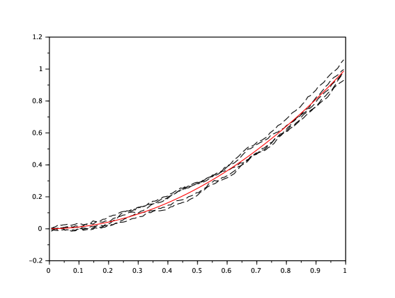
Figure 1. Plots of $5$ estimations (dashed black) of the true function $\texttt{b}_{0}$ (red) in Model (8) ($N=100$ copies).

Now, consider $H\in(1/2,1)$, $T=1$, $N=50$, $\Delta=\delta T$ with $\delta\in\mathbb{N}^{*}$, and the $T$-periodic (and then $(T+\Delta)$-periodic) function $b_{0}$ such that

$$b_{0}(t)=t^{2}\textrm{ $;$ }\forall t\in[0,T).$$

Note that, for every $i\in\{1,\dots,N+1\}$,

$$t_{i}(\Delta)=(i-1)(T+\Delta)=(i-1)(1+\delta)T.$$

For $n=50$, the fractional Brownian motion $B$, and then $X=b_{0}+Z$ with $Z=\sigma B$, are simulated along the dissection

$$\bigcup_{i=1}^{N}\left\{t_{i}(\Delta)+\frac{\ell T}{n}\textrm{ $;$ }\ell=0,\dots,n(1+\delta)\right\}\quad{\rm of}\quad[0,t_{N+1}(\Delta)].$$

So, for every $i\in\{1,\dots,N\}$, the process $X^{i}$ defined by (10) is computed along $\{\frac{\ell T}{n}\textrm{ $;$ }\ell=0,\dots,n\}$:

$$X_{\frac{\ell T}{n}}^{i}=X_{t_{i}(\Delta)+\frac{\ell T}{n}}-X_{t_{i}(\Delta)}\textrm{ $;$ }\ell\in\{0,\dots,n\}.$$

Again, $b_{0}$ is estimated by $\widehat{b}=\overline{X}$. Figure 2 shows the true function $b_{0}$ (red line) and 5 estimations obtained thanks to $\widehat{b}$ (dashed black lines) for two values of $H$ ($0.6$ and $0.9$) and a double forgetting period ($\delta=2$).

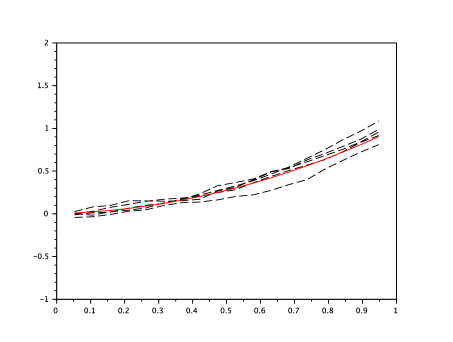
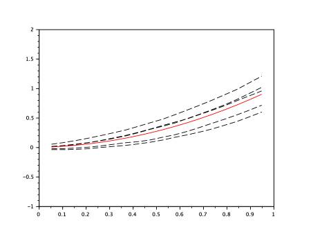
Figure 2. Plots of 5 estimations (dashed black) of the true function $b_{0}$ (red) in Model (10) for $\delta=2$ and $H=0.6,0.9$ ($N=50$ copies).

The experiment is repeated $100$ times for $\delta=2$, but also for a single forgetting period ($\delta=1$), and the means and standard deviations of ${\rm MISE}(\widehat{b})$ are stored in Table 1.

	$\delta=1$	$\delta=2$
$H=0.6$	$5\cdot 10^{-3}$ ($5.9\cdot 10^{-3}$)	$4.3\cdot 10^{-3}$ ($3.5\cdot 10^{-3}$)
$H=0.9$	$2.2\cdot 10^{-2}$ ($4.1\cdot 10^{-2}$)	$1.9\cdot 10^{-2}$ ($1.7\cdot 10^{-2}$)

Table 1. Mean and StD. (in parentheses) of ${\rm MISE}(\widehat{b})$ for $\delta=1,2$ and $H=0.6,0.9$ (100 repetitions).

Both Figure 2 and the columns of Table 1 show that for a fixed value of $\delta$, the mean and standard deviation of ${\rm MISE}(\widehat{b})$ are small but degrade when $H$ increases. Moreover, the rows of Table 1 show that for a fixed value of $H$, the mean and standard deviation of ${\rm MISE}(\widehat{b})$ improve when $\delta$ increases. These numerical findings were expected from Corollary 3.5.

4.2. Estimation in Model (4) via $\widehat{b}^{\prime}$

As in the first part of Section 4.1, $N=100$ independent Brownian motions $W^{1},\dots,W^{N}$ are simulated along the dissection $\{\frac{\ell T}{n}\textrm{ $;$ }\ell=0,\dots,n\}$ of $[0,T]$ with $T=1$ and $n=150$. Consider the $N$-dimensional process $\mathbf{Z}=(Z^{1},\dots,Z^{N})$ such that

$$\frac{1}{\sigma}\mathbf{Z}_{t}=\Gamma_{\star}^{\frac{1}{2}}\mathbf{W}_{t}\textrm{ $;$ }\forall t\in[0,T],$$

where $\sigma=0.5$, $\mathbf{W}=(W^{1},\dots,W^{N})$, and $\Gamma_{\star}=(\gamma^{|i-k|})_{i,k}$ with $\gamma\in(0,1)$. Clearly, $Z^{1},\dots,Z^{N}$ are $N$ correlated Brownian motions satisfying the condition (16), whose correlation increases with $\gamma$. For any $i\in\{1,\dots,N\}$, the solution $S^{i}$ of Equation (4) is simulated thanks to (5) with $X^{i}=b_{0}+Z^{i}$, where

$$b_{0}(t)=\frac{t^{2}}{2}-\frac{\sigma^{2}t}{2}\textrm{ $;$ }\forall t\in[0,T].$$

Then, the drift function $\texttt{b}_{0}=\frac{\sigma^{2}}{2}+b_{0}^{\prime}={\rm Id}_{[0,T]}$ in Equation (4) is estimated by

$$\widehat{\tt b}=\frac{\sigma^{2}}{2}+\widehat{b}^{\prime}=\frac{\sigma^{2}}{2}+\sum_{j=1}^{\widehat{m}}\mathcal{I}(\varphi_{j},\overline{X})\varphi_{j},$$

where $(\varphi_{1},\dots,\varphi_{N})$ is the $[0,T]$-supported trigonometric basis, and $\widehat{m}$ is selected in $\{2,\dots,12\}$ via (26).

Figure 3 shows the true function $\texttt{b}_{0}$ (red line) and 5 adaptive estimations obtained thanks to $\widehat{\tt b}$ (dashed black lines) for three values of $\gamma$ ($0$, $0.5$ and $0.75$).

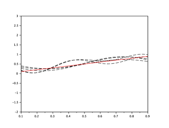
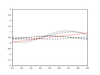
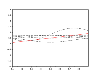
Figure 3. Plots of 5 adaptive estimations (dashed black) of the true function $\texttt{b}_{0}$ (red) in Equation (4) for $\gamma=0,0.5,0.75$ ($N=100$ copies).

The experiment is repeated $100$ times, and the means and standard deviations of ${\rm MISE}(\widehat{\tt b})$ and $\widehat{m}$ are stored in Table 2.

$\gamma$	$0$	$0.5$	$0.75$
Mean ${\rm MISE}(\widehat{\tt b})$	$1.1\cdot 10^{-2}$	$4.3\cdot 10^{-2}$	$8.1\cdot 10^{-2}$
StD. ${\rm MISE}(\widehat{\tt b})$	$0.2\cdot 10^{-2}$	$2.7\cdot 10^{-2}$	$2.7\cdot 10^{-2}$
Mean $\widehat{m}$	$3.4$	$2.4$	$2.2$
StD. $\widehat{m}$	$0.894$	$0.548$	$0.447$

Table 2. Means and StD. of ${\rm MISE}(\widehat{\tt b})$ and $\widehat{m}$ (100 repetitions).

Both Figure 3 and Table 2 show that the mean and standard deviation of ${\rm MISE}(\widehat{\tt b})$ are small (of order $10^{-2}$) when $\gamma=0$ (i.e. $Z^{1},\dots,Z^{N}$ are independent), but degrade when $\gamma$ increases, which was expected from Theorem 3.12. Moreover, for all considered values of $\gamma$, the standard deviation of $\widehat{m}$ is lower than $1$ (see Table 2), meaning that our model selection procedure (26) is quite stable.

References

- [1] Baraud, Y., Comte, F. and Viennet, G. (2001). Model Selection for (Auto-)Regression with Dependent Data. ESAIM:PS 5, 33-49.
- [2] Bunea, F., Ivanescu, A.E. and Wegkamp, M.H. (2011). Adaptive Inference for The Mean of a Gaussian Process in Functional Data. Journal of the Royal Statistical Society B 73(4), 531-558.
- [3] Cao, G. (2014). Simultaneous Confidence Bands for Derivatives of Dependent Functional Data. Electronic Journal of Statistics 8, 2639-2663.
- [4] Comte, F., Coutin, C. and Renault, E. (2012). Affine Fractional Stochastic Volatility Models. The Annals of Finance 8, 337-378.
- [5] Comte, F. and Genon-Catalot, V. (2020). Nonparametric Drift Estimation for I.I.D. Paths of Stochastic Differential Equations. The Annals of Statistics 48(6), 3336-3365.
- [6] Comte, F. and Marie, N. (2023). On a Projection Estimator of the Regression Function Derivative. Journal of Nonparametric Statistics 35(4), 773-819.
- [7] Denis, C., Dion, C. and Martinez, M. (2021). A Ridge Estimator of the Drift from Discrete Repeated Observations of the Solution of a Stochastic Differential Equation. Bernoulli 27, 2675-2713.
- [8] DeVore, R.A. and Lorentz, G.G. (1993). Constructive Approximation. Springer.
- [9] Donnet, S. and Samson, A. (2013). A Review on Estimation of Stochastic Differential Equations for Pharmacokinetic/Pharmacodynamic Models. Advanced Drug Delivery Reviews 65, 929-939.
- [10] Duellmann, K, Küll, J. and Kunisch, M. (2010). Estimating Asset Correlations from Stock Prices or Default Rates - Which Method is Superior? Journal of Economic Dynamics & Control 34, 2341-2357.
- [11] Ferraty, F. and Vieu, P. (2006). Nonparametric Functional Data Analysis. Springer.
- [12] Friz, P. and Victoir, N. (2010). Multidimensional Stochastic Processes as Rough Paths: Theory and Applications. Cambridge University Press.
- [13] Ghale-Joogh, H.S. and Hosseini-Nasab, S.M.E. (2020). On Mean Derivative Estimation of Longitudinal and Functional Data: from Sparse to Dense. Statistical Papers 62, 2047-2066.
- [14] Ibragimov, I.A. and Rozakov, Y.A. (1978). Gaussian Random Processes. Springer.
- [15] Kassi, O. and Patilea, V. (2025). Optimal Inference for the Mean of Random Functions. arXiv:2504.11025.
- [16] Kubilius, K., Mishura, Y. and Ralchenko, K. (2017). Parameter Estimation in Fractional Diffusion Models. Springer.
- [17] Kutoyants, Y. (2004). Statistical Inference for Ergodic Diffusion Processes. Springer.
- [18] Marie, N. (2023). Nonparametric Estimation for I.I.D. Paths of a Martingale Driven Model with Application to Non-Autonomous Financial Models. Finance and Stochastics 27(1), 97-126.
- [19] Marie, N. (2025). From Nonparametric Regression to Statistical Inference for Non-Ergodic Diffusion Processes. Springer.
- [20] Nualart, D. (2006). The Malliavin Calculus and Related Topics. Springer.
- [21] Privault, N. and Réveillac, A. (2008). Stein Estimation for the Drift of Gaussian Processes Using the Malliavin Calculus. The Annals of Statistics 36(5), 2531-2550.