Notions of Adiabatic Drift in the Quantized Harper model

Abstract

We study a quantized, discrete and drifting version of the Harper Hamiltonian, also called the finite almost Mathieu operator, which resembles the pendulum Hamiltonian but in phase space is confined to a torus. Spacing between pairs of eigenvalues of the operator spans many orders of magnitude, with nearly degenerate pairs of states at energies that are associated with circulating orbits in the associated classical system. When parameters of the system slowly vary, both adiabatic and diabatic transitions can take place at drift rates that span many orders of magnitude. Only under an extremely negligible drift rate would all transitions into superposition states be suppressed. The wide range of energy level spacings could be a common property of quantum systems with non-local potentials that are related to resonant classical dynamical systems. Notions for adiabatic drift are discussed for quantum systems that are associated with classical ones with divided phase space.

I Introduction

In this study we contrast and explore notions of adiabatic behavior for a drifting classical and associated quantum Hamiltonian system on a torus. An advantage of studying a quantized system on the torus is that it is finite dimensional, facilitating numerical calculations and potential applications in quantum computing. Finite dimensional quantum spaces are relevant for evolution of spin systems (e.g., Bossion et al. 8) that are studied in the context of chemistry and nuclear physics. The ability to estimate whether a system behaves adiabatically is relevant for implementing effective adiabatic quantum computation algorithms [1] which can be used to solve satisfiability and other combinatorial search problems and some optimization problems [32]. The system we study, the quantized Harper model, resembles the pendulum dynamical system and that model describes superconducting transmons [22, 5, 12], so our study is relevant for control of quantum computers that leverage these devices [9].

Complex classical dynamical systems, including multiple planet systems [30] and particles in a plasma [11], can exhibit resonant behavior that can be described with Hamiltonian models that resemble the pendulum. The classical pendulum Hamiltonian

$$H_{\rm pend}(p,\phi)=\frac{p^{2}}{2}-\epsilon\cos\phi$$ (1)

where momentum $p$ and angle $\phi$ are canonical coordinates that are functions of time $t$ and constant parameter $\epsilon$ describing the resonance strength sets the oscillation frequency at the bottom of the cosine potential well. This system exhibits two types of dynamical behavior: libration, where the angle $\phi(t)$ oscillates about zero, and circulation, where $\phi$ continuously increases or continuously decreases in time. In phase space, the two types of behavior are separated by an orbit, known as the separatrix, that has an infinite period and contains the hyperbolic fixed point located at $(p,\phi)=(0,\pi)$.

A more general version of the pendulum model of equation 1 depends upon three parameters $a,b,\epsilon$;

$$H_{\rm pend}(p,\phi)^{\prime}=a\frac{(p-b)^{2}}{2}-\epsilon\cos\phi.$$ (2)

The parameter $b$ shifts the locations of the fixed points. We consider the situation where the parameters $a,b,\epsilon$ are slowly varying in time. An example setting is the dynamics of a migrating moon or planet [6]. In celestial mechanics, the unperturbed system is expanded to second order in an action variable (giving the quadratic kinetic energy term). A gravitational perturbations from a planet is expanded in a Fourier series (giving $\phi$ dependent terms). A motivation for studying a system resembling the pendulum is that the Hamiltonian of a transmon in a resonator circuit QED setup takes the form of the Hamiltonian in equation 2 with momentum $p=n$ equal to the charge operator, the angle $\phi$ equal to the phase operator, the coefficient $a=4E_{C}$ with $E_{C}$ equal to the charging energy, the coefficient $\epsilon=E_{J}$, the Josephson energy and $b=n_{g}$ an offset charge [22, 5].

In classical Hamiltonian systems, Liouville’s theorem implies that adiabatic drift is associated with near conservation of an action variable which depends upon a contour or surface in phase space that encloses a constant phase space volume. However, a particle that nears a separatrix orbit as the system varies must enter a non-adiabatic dynamical regime because the period of the separatrix is infinite due to the presence of a hyperbolic fixed point. Overcoming this difficulty, the Kruskal-Neishtadt-Henrard (KNH) theorem [27, 21] relates the probability of transition between different phase space regions to the rates that the enclosed phase space volumes vary. In celestial mechanics this process is called resonance capture (e.g., [6, 42]). The capture probability computed via the Kruskal-Neishtadt-Henrard theorem is accurate only if the drift rate is slower than a dimensionally derived function of the resonance libration frequency which also describes the rate that orbits diverge from unstable fixed points [29]. Even though dynamics near the separatrix is not actually adiabatic, resonance capture is often described as an adiabatic process as it only occurs at a slow drift rate. Classical Hamiltonian dynamics is deterministic, rather than probabilistic. However the sensitivity of the dynamics near a hyperbolic fixed point contained in the separatrix orbit means that the asymptotic behavior of a distribution of orbits that crosses a separatrix is well described with a probability.

Notions of adiabatic drift differ between classical and quantum systems. In a quantum system, adiabatic variation is often used to describe a slowly varying Hamiltonian operator that drifts sufficiently slowly that a system initially in an eigenstate of the operator remains in an eigenstate of the Hamiltonian operator [7]. This principle is known as the adiabatic theorem. When the system drifts fast enough that a transition from one eigenstate to another takes place, the transition is called diabatic. The Landau-Zener model [44, 41, 39] for a drifting 2-state quantum system gives an expression for the probability of a diabatic transition as a function of the drift rate and the minimum energy difference between the two states at their closest approach.

Using Bohr-Sommerfeld quantization and the WKBJ semi-classical limit, Stabel and Anglin [36] showed that a quantum version of the Kruskal-Neishtadt-Henrard theorem holds for a drifting quantized double well potential. In this system, as the Hamiltonian operator slowly varies, there is a lattice of of avoided energy level crossings in the vicinity of the separatrix of the associated classical system. Each energy level crossing can be approximated via the two-level Landau-Zener model, giving a connection between the probabilities of transition between quantum states and the growth rates of phase space areas [36].

We build upon the work by Stabel and Anglin [36], however, instead of a varying double well potential and using a semi-classical limit, we examine a quantized system on the torus that resembles the pendulum, known as the Harper model, which is equivalent to a discrete version of the Mathieu operator (arising from Schrödinger’s equations for the quantum pendulum) called the finite almost Mathieu operator [37]. An advantage of using a discrete or finite dimensional operator is that we can explicitly calculate the energy differences between eigenstates. The classical Hamiltonian of the Harper model [19], describing the motion of electrons in a 2-dimensional lattice in the presence of a magnetic field, is

$$H_{\rm Harper}(p,\phi)=a\cos p+\epsilon\cos\phi,$$ (3)

with canonical coordinates $p,\phi\in[-\pi,\pi]$ in a doubly periodic domain and real coefficients $a,\epsilon$. For small momentum $p$, a constant minus the kinetic term is $1-\cos p\approx p^{2}/2$ which resembles kinetic energy, so at small $p$, the Harper model exhibits dynamics similar to the pendulum. An advantage of studying the Harper Hamiltonian is that it can be quantized in a finite dimensional complex vector space. For this model, because it is finite dimensional and can be simply written in terms of clock and shift operators (see appendix A.1), it is straight-forward to compute its eigenvalues to high precision and calculate the distance between eigenvalues during avoided crossings. For the Harper model, quantization via Bohr-Sommerfeld quantization, by using two mutually unbiased bases related via Fourier transform to describe the operators $\hat{p},\hat{\phi}$, or with a point operator constructed from discrete coherent state analogs to carry out Wigner-Weyl quantization is discussed by Quillen and Miakhel [31].

As we did in equation 2 for the pendulum, we modify the Harper model with an additional parameter $b$ so that the libration regions can be shifted, giving

$$H_{\rm Harper}(p,\phi)^{\prime}=a\cos(p-b)+\epsilon\cos\phi.$$ (4)

Figure 1 illustrates level curves of this Hamiltonian. The two panels in this figure show how the center of the librating region is shifted by the parameter $b$. The parameter $\epsilon$ controls the width of the librating regions. If $|\epsilon|<|a|$ and $a,\epsilon\neq 0$, phase space is divided into three regions, two with orbits that librate about $\phi=0$ or $\pi$, and a circulating region where orbits cover all possible values of $\phi$. The energies of the separatrix orbits can be found by identifying the hyperbolic fixed points. The separatrix orbits have

$$E_{sep}=\pm(|a|-|\epsilon|)$$ (5)

and there are two of them if $|a|\neq|\epsilon|$ and $a,\epsilon\neq 0$. If $|a|=|\epsilon|\neq 0$, the circulating region vanishes and there is only one separatrix energy which separates two librating regions.

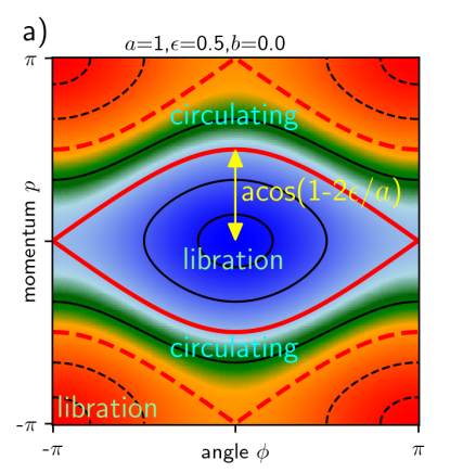
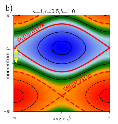
Figure 1: Level curves in phase space of the classical Harper Hamiltonian of equation 4. Thick red level curves show the two separatrix orbits. Negative energies are shown with dotted contours. A comparison between left and right panels illustrates how the parameter $b$ shifts the center of the librating regions. Parameters for the model are shown on the top of each panel. Librating and circulating regions are annotated on the left panel. The parameter $\epsilon$ sets the width of the librating region.

For the quantized version of the Harper model, we work in an $N$ dimensional complex vector space that has an inner product. The quantized version of equation 4 is the Hermitian operator

$$\hat{h}=a\cos(\hat{p}-b)+\epsilon\cos\hat{\phi}$$ (6)

with operators $\hat{p}$ and $\hat{\phi}$ defined in section A.1 (also see [31]).

II The eigenvalues of the Harper operator

In this section we discuss how the set of eigenvalues or spectrum of the operator of equation 6 depends on the parameters $b,\epsilon$. For $a=1$, $b=0$, and $\epsilon=0$, the Hamiltonian operator is equal to $\cos\hat{p}$ so its eigenvalues are $\cos\left(\frac{2\pi j}{N}\right)$ with index $j\in\{0,1,....,N-1\}$. For most values of index $j$, eigenvalues have multiplicity 2. With dimension $N$ odd there is a single non-degenerate eigenvalue but for $N$ even there are two. In Figure 2 for different values of $\epsilon$ we compute and plot the spectrum of $\hat{h}$. For $\epsilon>0$, the eigenvalue degeneracy is broken, as can be seen on the left side of Figure 2 where pairs of eigenvalues split as $\epsilon$ increases.

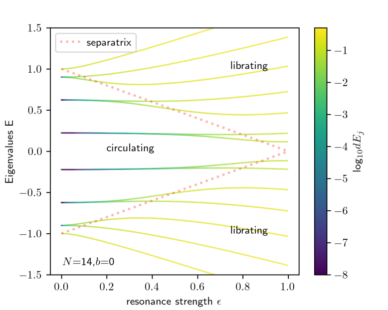
Figure 2: Eigenvalues of the Hamiltonian operator in equation 6 for different values of resonance strength $\epsilon$. Parameters $b=0$, $a=1$ remain fixed and the dimension $N=14$. For $\epsilon>0$, eigenvalues are in nearly degenerate pairs within the circulating region but well separated in the region associated with classically librating orbits. The red dotted line shows the separatrix energy values for the associated classical model (equation 5). As the resonance strength $\epsilon$ increases, the area within the separatrix orbit increases and more eigenstates are in the region associated with librating orbits. The colorbar gives an estimate for the log of the distance to the nearest eigenvalue for each eigenvalue and at each value of $\epsilon$, however the colorbar is truncated at -8 so the spacings can be smaller than shown with navy blue points.

At the bottom of the cosine potential well, and at low energy, the spectrum of the Harper operator resembles that of a harmonic oscillator which has evenly spaced eigenvalues. For $N$ even there is a reflective symmetry in the spectrum of $\hat{h}$ about an energy of 0, (see appendix A.4). In Figure 2 we have drawn the energies of the separatrix for the associated classical system (given in equation 5) with dotted red lines. The spectrum consists of nearly degenerate eigenvalue pairs in the circulating region and the eigenvalues are well separated in the librating regions.

The lower half of Figure 2 resembles Figure 1 by Doncheski and Robinett [17] showing the spectrum of the quantum pendulum (equivalently, the eigenvalues of the Mathieu function) also as a function of strength parameter (also see [16], https://dlmf.nist.gov/28.2). The spectrum of the quantum pendulum also exhibits nearly degenerate pairs of states above its separatrix and distinct and well separated energy states within its potential well [17]. The dichotomy of energy level spacing in the Harper operator is not caused by confinement to a torus as it is also present in the quantized pendulum with momentum $p\in[-\infty,\infty]$. Similarity between the spectrum of the Harper operator and the quantized pendulum is discussed in more detail in appendix LABEL:ap:mathieu.

The spectrum of the operator $\hat{h}$ in dimension $N$ at particular values of the parameters $a,b,\epsilon$ is the set of eigenvalues $\{\lambda_{j}\}$ indexed by $j\in\{0,...,N-1\}$. For each spectrum computed with a specific value of parameters $a,b,\epsilon$ and for each eigenvalue $\lambda_{j}$ we define the distance in energy to the nearest eigenvalue;

$$dE_{j} ={\rm min}_{k\neq j}|\lambda_{j}-\lambda_{k}|.$$ (7)

The log${}_{10}(dE_{j})$ of the eigenvalue (or energy) spacings of the Hamiltonian operator in equation 6 are shown in color in Figure 2 and with numerical values corresponding to the colorbar on the right. The colorbar does not extend below $dE_{j}=10^{-8}$, but the spacings decrease to zero on the left side as $\epsilon\to 0$ where pairs of eigenvalues become degenerate. Figure 2 shows that the Harper operator exhibits an extremely wide range of spacings between its eigenvalues.

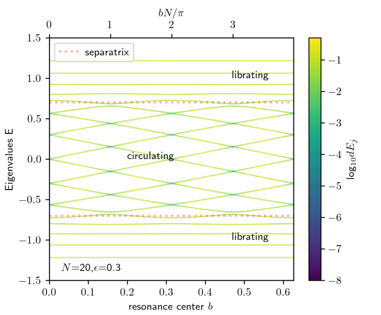
Figure 3: Eigenvalues of the Hamiltonian operator in equation 6 for different values of parameter $b$. This figure is similar to Figure 2 except $b$ varies instead of $\epsilon$, and dimension $N=20$. The parameter $\epsilon=0.3$ is fixed. Energy levels in the librating regions do not vary quickly as $b$ varies. However, energy levels in the circulating regions exhibit a lattice of avoided crossings. The axis on the top shows $b$ in units of $\pi/N$. Avoided crossings in the circulating region occur where $b$ is a multiple of $\pi/N$. A heuristic explanation for the dichotomy is given in section II.2.

Figure 3 also shows the spectrum of the Hamiltonian operator in equation 6, however here we vary the $b$ parameter while the resonance strength $\epsilon$ remains fixed. Figure 3 shows that the energy levels in the librating regions remain separated and do not vary very much. However, energy levels in the circulating region show a lattice of crossings, that are avoided, as we discuss below. By avoided we mean that the two energy levels don’t actually cross, rather they approach each other then diverge from each other. The avoided crossings have extrema at $b$ equal to a multiple of $\pi/N$, and for these values energy levels in the circulating region are nearly degenerate. The lattice of avoided crossings was also seen near a separatrix in the time-dependent double well potential model studied by Stabel and Anglin [36].

The lattice of avoided crossings seen in the circulating region in Figure 3 implies that the operator $\hat{h}(a,b,\epsilon)$ (equation 6) obeys symmetries that are described in more detail in appendix A and which we now summarize. With $a,\epsilon$ fixed, the spectrum is identical if $b$ is shifted by $2\pi/N$ (theorem A.3). The spectrum has reflective symmetry about $b$ for $b$ a multiple of $\pi/N$ (theorems A.5 and A.8). For $N$ even, as shown in Figures 2 and 3, the spectrum itself is symmetrical about an energy of zero (theorem A.15). Degeneracy of eigenvalues is explored in appendix A.6. The eigenvalues are distinct if $b$ is not a multiple of $\pi/N$ (theorem A.18). Numerical calculations show that the spacing between nearly degenerate pairs of eigenvalues is smallest for $b$ a multiple of $\pi/N$ and that eigenvalues are distinction $a,\epsilon\neq 0$ as long as $N$ is not a multiple of 4. There are two zero eigenvalues in the special case of $N$ a multiple of 4 (lemma LABEL:th:zeros). The near approaches of pairs of eigenvalues at $b$ multiples of $\pi/N$ could be related to two symmetries that are present for $b$ a multiple of $\pi/N$ (see commutators in equations 54 and 59 of theorems A.11, A.12). The fact that spacings are a minimum for specific values of $b$ aids in computing the minimum distance between eigenvalues for drifting systems and is another advantage of exploring a simple system such as the Harper operator. Many of the symmetries associated with the lattice of avoided crossings are obeyed by operators that have potentials that are more general than the $\cos\hat{\phi}$ potential in the Harper operator, as discussed in appendix LABEL:ap:other.

With both $b$ and $\epsilon$ increasing, there is both a lattice of avoided crossings in the circulating region and an increase in the number of eigenstates in the libration region, as shown in Figure 4. In the associated classical system, the area in phase space of the librating region grows while that in the circulating region shrinks. At an appropriate drift rate, a system begun in an circulating eigenstate would experience diabatic crossings within the circulating region, and then when approaching the separatrix could adiabatically remain in an eigenstate that starts to librate within the potential well, as described for the time dependent double well potential system by Stabel and Anglin [36]. This process is the quantum equivalent of the classical process known as resonance capture.

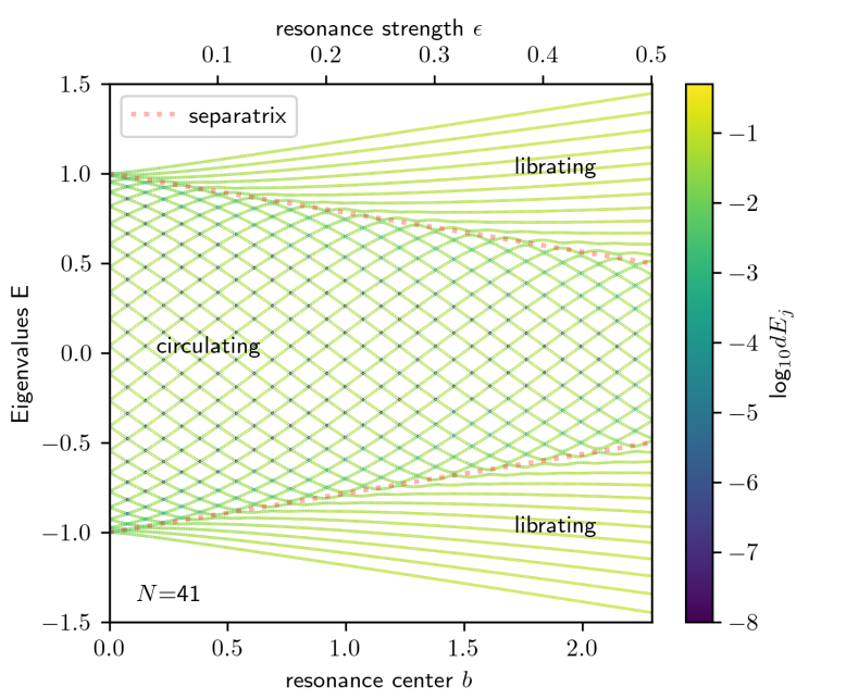
Figure 4: Eigenvalues of the Hamiltonian operator in equation 6 for different values of parameters $\epsilon,b$ where both $\epsilon,b$ together increase linearly with values shown on the top and bottom axes. This Figure is similar to Figure 2 except the parameters $b,\epsilon$ both vary and dimension $N=41$. As the resonance strength (set by $\epsilon$) increases, more eigenstates are associated with librating orbits.

II.1 Spacing between eigenvalues

The Landau-Zener two-level model shows that during an avoided crossing the probability of a diabatic transition is a function of the drift rate and the minimum energy difference between the two states at their closest approach. When the parameters describing the Harper operator are time dependent, then the probability of diabatic transitions depends on the distances between energy levels. In this section we examine in more detail the near degeneracies seen in Figures 2 – 4.

To compute the eigenvalues in Figures 2 – 4 we used routines available in the numpy package within Python which uses the LAPACK linear algebra library. The distances between pairs of eigenvalues were so small that were were concerned about the accuracy of the calculation with the LAPACK linear algebra library. To check the accuracy of the calculation, we computed eigenvalues values to a higher level of precision using the Python library for real and complex floating-point arithmetic with arbitrary precision mpmath [38]. In Figure 5 we show the smallest distance between eigenvalues for $\hat{h}$ (equation 6) with $a=1$ for fixed values of $\epsilon=0.5$, $b=0$ but as a function of $N$ and computed to 50 digits of precision using the mpmath library. This is about 20 digits more accurate than computed with the conventional LAPACK library.

Figure 5 confirms that the distance between pairs of eigenvalues is non-zero and small within the circulating region and smallest in the center of the circulating region where the eigenstate energy is near zero. With the higher level of precision we find that the eigenvalues are not degenerate except in the case of $N$ a multiple of 4, in which case there is a pair of zero eigenvalues. That there is a pair of zero eigenvalues for $N$ a multiple of 4 is shown using the determinant of the operator computed in appendix LABEL:ap:det and with lemma LABEL:th:zeros). Within the circulating region, the distance between the pairs of eigenvalues decreases over orders of magnitude. The range of spacings between eigenvalues is remarkably vast and increases with increasing dimension $N$. In the high energy limit of the quantized pendulum which resembles the quantum rotor, and with increasing distance from the separatrix, the distance in energy between pairs of eigenvalues also approaches zero (e.g., [17], also see appendix LABEL:ap:mathieu). For our system, because the circulating region is bounded on both sides by potential wells, the minimum spacing between eigenvalues is found in the center of the circulating region.

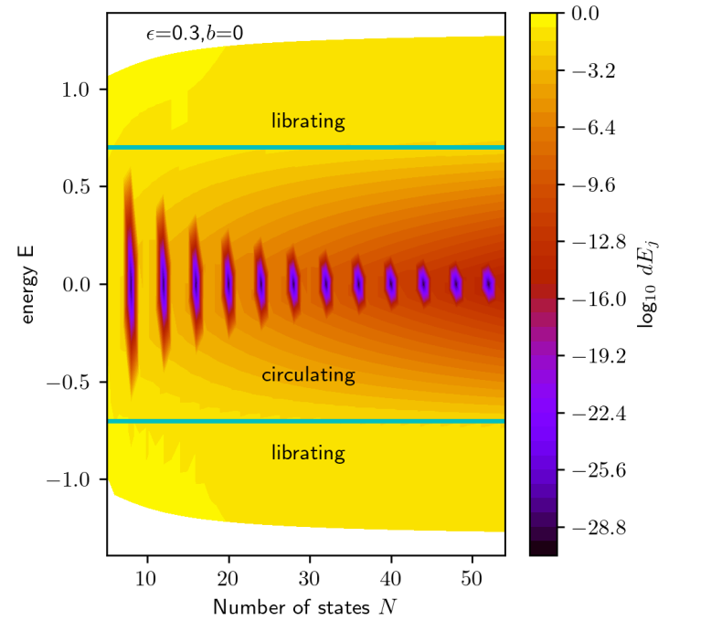
Figure 5: We show the smallest distance, in color and with colorbar shown on the right, between neighboring eigenvalues as a function of eigenvalue (on the $y$-axis) and as a function of the number of states $N$ in the Hilbert space on the $x$-axis for the Hamiltonian operator of equation 6 with $a=1,b=0$. The parameter $\epsilon$ is fixed and printed on the plot. The cyan thick lines show the energies of the separatrix classical orbits. For energies between the separatrix orbits there are near degeneracies between pairs of eigenstates. The pairs of eigenvalues are not the same except for $N$ a multiple of 4 and in that case only for a pair of zero eigenvalues.

The spacing between eigenvalues at different values of $\epsilon$ for two different values of $N$, are shown in Figure 6. This figure also illustrates that the minimum distance between pairs of eigenvalues is found near an energy of 0 in the circulating region. The colorbar is in a log scale. Level contours within the circulating region are nearly linear suggesting that the energy level spacing in the circulating region is approximately a power of $\epsilon$.

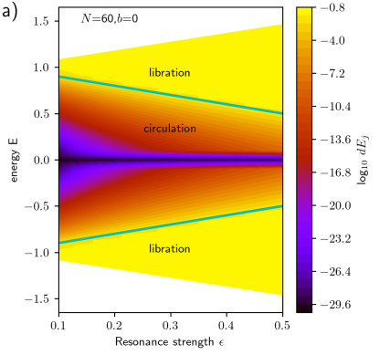
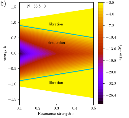
Figure 6: a) We show the spacing, in color and with colorbar shown on the right, between neighboring eigenvalues as a function of eigenvalue (on the $y$ axis) and as a function of the parameter $\epsilon$ (on the $x$-axis) for the Hamiltonian of equation 6 with $a=1$, $b=0$. The number of states is shown on the top left. For $N$ a multiple of 4, there are two zero energy eigenvalues. b) Similar to a) but for an odd dimension $N$. The spacing between eigenvalues increases as $\epsilon$ increases and for each $\epsilon$ is smallest in the center of the circulating region. The distance between neighboring eigenvalues spans many orders of magnitude.

How the distance between nearby energy levels depends on eigenvalue index is shown in Figure 7 where we plot the eigenvalue spacing $dE_{j}$ (defined in equation 7), as a function of eigenvalue index, with index $j$ in order of increasing eigenvalue. Figure 7 illustrates that the distance between the pairs of nearly degenerate eigenvalues drops rapidly in the circulating region. The drop is nearly linear on a log plot implying that the spacing depends on a power of the index, with exponent dependent upon dimension $N$ and $\epsilon$. In Figure 7 we show eigenvalue spacing $N=50$ even but not a multiple of 4, and $N=52$ which is a multiple of 4. The spacings are similar except at $j/N\sim 0.5$ where in the $N=52$ (divisible by 4) case there is a zero eigenvalue of multiplicity 2 giving $dE_{j}=0$.

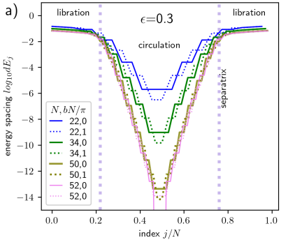
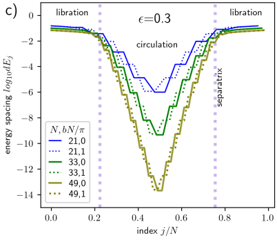
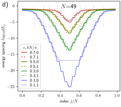
Figure 7: a) The log${}_{10}$ of spacings $dE_{j}$ between neighboring energy levels is shown as a function of index $j$ of ordered energy levels for different values of dimension $N$, for $N$ even, and at resonance strength $\epsilon=0.3$ for the operator $\hat{h}(a,b,\epsilon)$ with $a=1$. The solid and dotted lines show spacings $dE_{j}$ computed for $b=0$ and $b=\pi/N$, respectively. The indices that have energy near that of the separatrices are shown with vertical dotted lines. b) Similar to a) except we show spacings for even $N=50$ for 4 different values of $\epsilon$. c) Similar to a) except for three different values of $N$ odd. d) Similar to b) except we show spacing for odd $N=49$. These figures illustrate that the spacing between pair of eigenvalues drops within the circulating region approximately as a power law.

The minimum distance between any pair of eigenvalues is reached at the center of the circulating region. Figure 8 shows the minimum distance between any pair eigenvalues as a function of $N$ and $\epsilon$ for $b=0$ and $b=\pi/N$ and for $N$ even but not a multiple of 4 and $N$ odd. We find that the minimum distance is approximately given by

$$dE_{min}\sim\begin{cases}\epsilon^{\frac{(N-1)}{2}}\frac{3}{N}&\text{if }N\text{ odd }\\ \epsilon^{\frac{(N-2)}{2}}\frac{5}{N}&\text{if }N\text{ mod }4=2\\ 0&\text{if }N\text{ mod }4=0\end{cases}.$$ (8)

These functions are plotted on Figure 8 which shows that they approximately describe the minimum spacing computed numerically. Low order perturbative expansion techniques, which we use in the next section, are often used to estimate energy level spacings (e.g., [43]). However, the power of $\epsilon$ in equation 8 is high, so a low order perturbative expansion would fail to estimate the minimum spacing between energy levels in the Harper operator. Using the characteristic polynomial of the operator $\hat{h}(1,0,\epsilon)$, we give a rough derivation of equation 8 in appendix LABEL:ap:min_spacing.

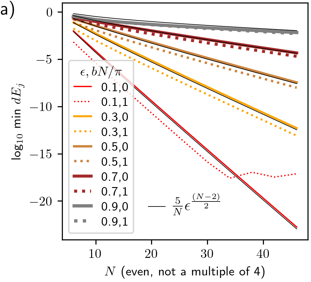
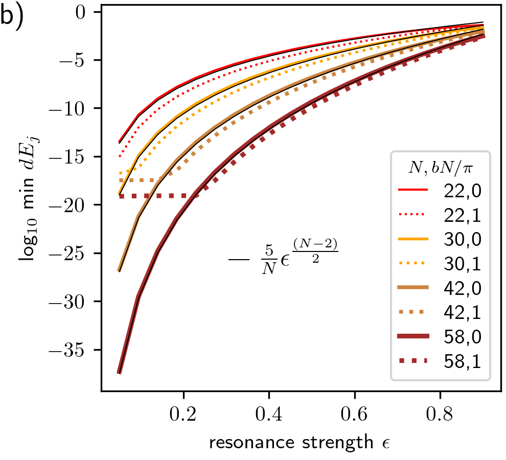
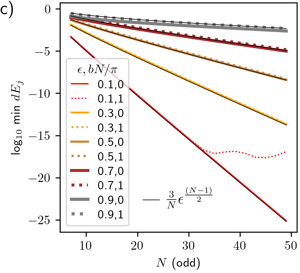
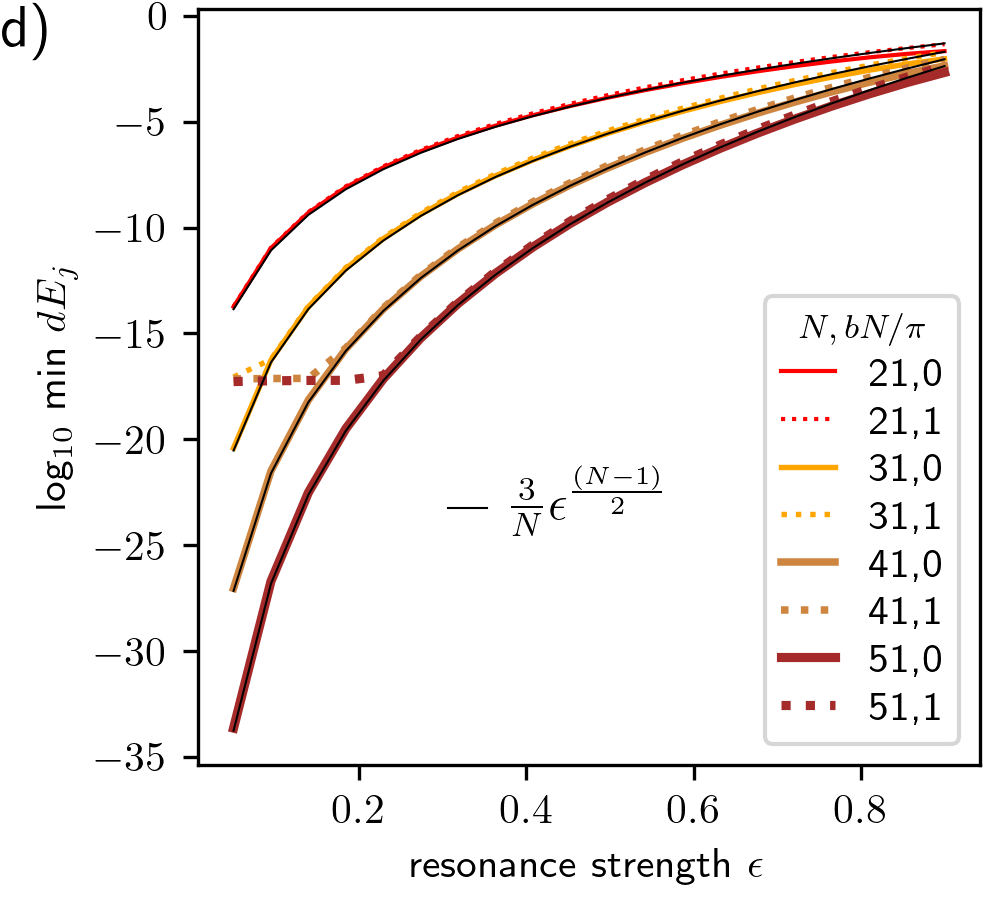
Figure 8: a) The log${}_{10}$ of the minimum spacing between eigenvalues (min $dE_{j}$) for the operator $\hat{h}(a,b,\epsilon)$, with $a=1$, as a function of $N$ for $N$ even but not a multiple of 4. We show the minimum space for different values of resonance strength $\epsilon$. Solid lines have $b=0$ and dotted lines $b=\pi/N$. The thin black lines show the estimate for the minimum gap given by equation 8. b) Similar to a) except as a function of resonance strength $\epsilon$. c) Similar to a) except for $N$ odd. d) Similar to b) except for $N$ odd.

II.2 Heuristic analogies for the sensitivity of the energy levels to the parameter $b$

In our finite dimensional space and for small resonant strength $\epsilon$, an energy level of 0 is in the circulating region and is above the top of the cosine potential well. We approximate the Hamiltonian of equation 6 (with $a=1$) as

$$\hat{h}(1,b,\epsilon)\approx\cos(\hat{p}-b)$$ (9)

which has eigenvalues

$$E_{k}(b)=\cos\left(\frac{2\pi k}{N}-b\right)$$ (10)

for $k\in\{0,1,\ldots,N-1\}$. Equivalently we can take $k\in-(N/2-1),\dots,N/2$ if $N$ is even or $k\in\{-(N-1)/2,\ldots,0,\ldots(N-1)/2\}$ if $N$ is odd. For $b=0$ most energy levels have multiplicity 2 as $E_{k}(0)=E_{-k}(0)$. For $b\neq 0$, $k>0$, energy levels are split by

$$E_{k}(b)-E_{-k}(b)=2\sin\left(\frac{2\pi k}{N}\right)\sin b.$$ (11)

For small $b$ the splitting between energy levels is first order in $b$. The energy levels diverge as $b$ increases.

In contrast, at the bottom of the potential well in the Harper model the Hamiltonian can be approximated by a harmonic oscillator with Hamiltonian $\hat{h}=\hat{a}^{\dagger}\hat{a}+{\rm constant}$ where $\hat{a}^{\dagger},\hat{a}$ are raising and lowering operators. The energy spectrum is a non degenerate ladder spectrum $E_{n}=n+{\rm constant}$ with $n$ a non negative integer. The eigenstates $\ket{n}$ obey $a^{\dagger}a\ket{n}=n\ket{n}$. A shift associated with parameter $b$ can be modeled with a perturbation $\hat{V}=b\hat{p}=\frac{b}{\sqrt{2}i}(\hat{a}-\hat{a}^{\dagger})$. First order perturbations vanish as $\bra{n}\hat{V}\ket{n}=0$. The perturbation gives second order perturbations to the energy levels

$$E_{n}(b) \approx n+\frac{b^{2}}{2}\Bigg{(}\frac{|\bra{n+1}(a-a^{\dagger})\ket{n}|^{2}}{-1}$$

$$\qquad+\frac{|\bra{n-1}(a-a^{\dagger})\ket{n}|^{2}}{1}\Bigg{)}$$

$$\approx n-\frac{b^{2}}{2}+{\cal O}(b^{3}).$$ (12)

The result is a shift in the spectrum that to second order in $b$ does not affect the energy spacing between eigenstates.

These examples heuristically illustrate why the energy levels do not strongly vary in the librating regions as $b$ varies but are quite sensitive to $b$ in the circulating regions.

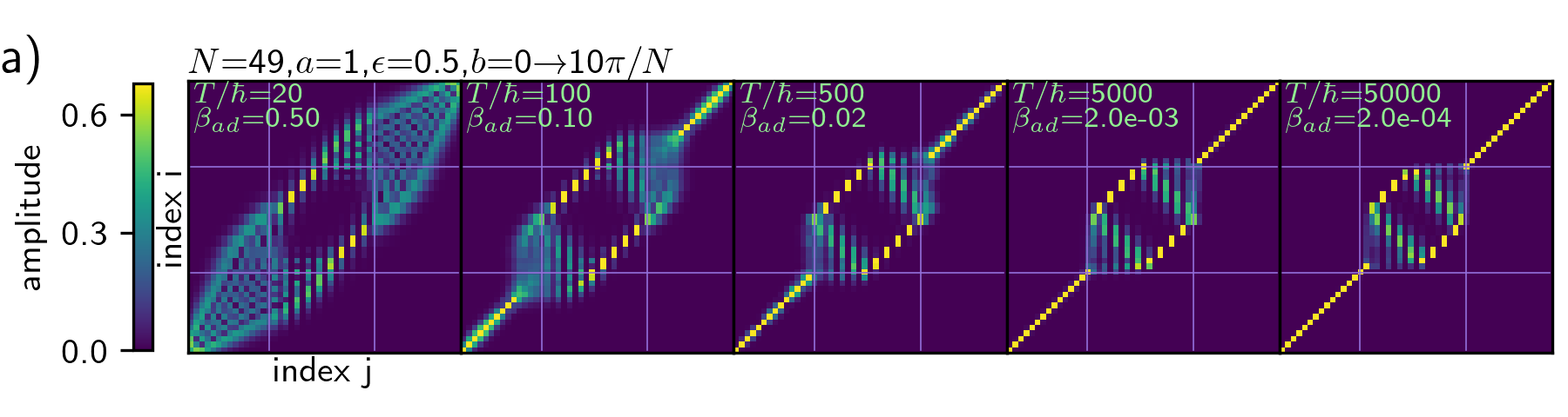
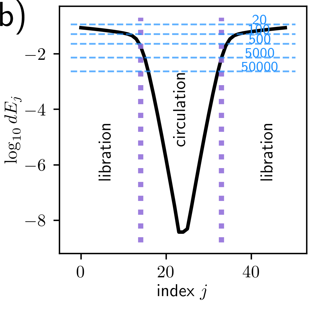
Figure 9: a) We show the amplitudes of the transition matrix $A_{ij}=|\bra{w_{j}}U(0,T)\ket{v_{i}}|$ as an image. The amplitudes are computed for different durations $T$ using time dependent Hamiltonian operator $\hat{h}(a,b(t),\epsilon)$ (in the form of equation 6) with $a,\epsilon$ fixed but with $b$ drifting linearly in time, initially at $b=0$ and reaching a value of $10\pi/N$. The dimension $N=49$. Indices in the transition matrix are ordered so that eigenvalues are increasing to the right and upward. The set of eigenstates $\ket{v_{i}}$ are those of the operator $\hat{h}$ initially and the set of eigenstates $\ket{w_{j}}$ are those of the operator at the final time. Each panel shows the transition matrix amplitude computed for different durations of drift but for the same total change in system parameters. The transition matrix contains a 1 if the system remains in an eigenstate. If the amplitude is between 0 and 1 then transitions can occur. In the leftmost panel, the drift rate is sufficiently fast that transitions take place in the librating region but transitions are diabatic within the circulating region near the center of the image. b) The minimum distance between energy levels $dE_{j}$ (defined in equation 7) for the operator $\hat{h}$ is shown on the right. The indices with eigenvalues nearest the separatrices are shown with dotted purple vertical lines. For each drift rate shown in panel a), horizontal blue dashed lines show the spacing that would give a probability of about 1/2 for a diabatic transition estimated using the Landau-Zener model (using equation LABEL:eqn:de_min_half). This figure illustrates that the system undergoes transitions for all the drift rates we used, and would not be completely adiabatic (and transition-less) unless the drift duration was 5 orders of magnitude longer than our longest and slowest integration.

III Drifting the quantized Harper model

The near degeneracy of pairs of eigenstates for the Harper operator affects the adiabatic behavior of the drifting quantized system. A slowly varying quantum system with Hamiltonian operator $\hat{h}(t)$ a function of time $t$ is described with the unitary transformation, called a propagator,

$$\hat{U}(t,t_{0})={\cal T}e^{-\frac{i}{\hbar}\int_{t_{0}}^{t}\hat{h}(t)dt}$$ (13)

where $\cal T$ denotes time ordering for each portion of the integral and $\hbar$ is Planck’s constant. A system initially at time $t_{0}$ in quantum state $\ket{\psi_{0}}$ would be in state $\hat{U}(t,t_{0})\ket{\psi_{0}}$ at a later time $t$.

We consider the time dependent Hamiltonian operator $\hat{h}(t)=\hat{h}(a,b(t),\epsilon(t))$ with operator $\hat{h}(a,b,\epsilon)$ equal to the Harper operator (equation 6). We allow parameters $b$ and $\epsilon$ to drift linearly in time, and fix $a=1$.

If the system drifts adiabatically, then a system begun in an eigenstate remains in an eigenstate. We denote $\ket{v_{i}}$ to be the eigenstates of the initial Hamiltonian $\hat{h}(t_{0})$ and $\ket{w_{j}}$ to be eigenstates of the final Hamiltonian $\hat{h}(t_{0}+T)$ where $T$ is the duration of the drift. With the two sets of eigenstates, we compute a matrix of transition amplitudes

$$A_{ij}=|\bra{w_{j}}\hat{U}(t_{0},t_{0}+T)\ket{v_{i}}|.$$ (14)

If the system drifts sufficiently adiabatically, the transition matrix $A_{ij}$ would only contain 1s and zeros as a system begun in an eigenstate would remain in an eigenstate.

III.1 Varying the resonance center

Figure 9a shows transition matrices computed for a drifting system with $\hat{h}(a,b(t),\epsilon)$ (defined in equation 6) with parameters $a,\epsilon$ fixed and $b$ varying linearly with time ($\frac{db}{dt}$ is constant) and initial $b(t=0)=0$. We compute the propagator $U(0,T)$ (equation 13) with drift duration $T$ and for different drift durations. The total change in the $b$ parameter is $\Delta b=10\frac{\pi}{N}$ and it is the same for each computed propagator but the duration $T$ of the drift differs in each panel in Figure 9a. To construct the transition matrix, eigenstates are sorted in order of increasing energy. The transition matrix is shown as a color image with the color of each pixel indexed by $i,j$, corresponding to the specific value of $A_{ij}$. The vertical axis gives the index $i$ of the initial eigenstates and the horizontal axis is the index of $j$ the final eigenstates. The indices of the states nearest the separatrix energies are shown with thin red horizontal and vertical lines.

Figure 9b shows the minimum spacing between pairs of eigenvalues reached as a function of index during the entire duration of the drift. Pairs of eigenvalues undergo different close approaches at $b$ an even multiple of $\pi/N$ and at $b$ an odd multiple of $\pi/N$, so the smallest distance shown is the minimum taking into account both types of avoided crossings. The indices of energies nearest the separatrix energy are shown on the plot with red dotted lines. As expected, the minimum distance between eigenvalues is smallest in the center of the circulating region. Horizontal lines on this plot show an estimate (derived in appendix LABEL:ap:LZ) based on the Landau-Zener model for the energy spacing between two states that would have a diabatic transition probability of 1/2 (computed with equation LABEL:eqn:de_min_half). A horizontal line is shown for each of the drift durations $T$ shown in Figure 9a and the duration $T$ values are labelled on top of each line.

Figure 9a shows that at rapid drift rates (with short duration for the drift), transitions take place between eigenstates in the librating region, whereas in the inner part of the circulating region there are diabatic transitions. At intermediate drift rates ($T/\hbar=500,5000$), transitions are suppressed in the librating regions where the dynamical behavior is adiabatic and some transitions can take place in the outer parts of the circulating region. With decreasing drift rate, the diabatic transition region in the center of the circulating region shrinks. However, Figure 9b shows that the drift rate would need to be about 5 orders of magnitude lower than our longest integration to ensure that no transitions take place and that the system drifts adiabatically for any initial state.

We compare the drift rates for $b$ shown in Figure 9 to the adiabatic limit for resonance capture estimated for the classical pendulum (following Quillen [29]). The KNH theorem holds and the classical system is said to be drifting adiabatically if $\dot{b}\ll\omega_{0}^{2}$ [29] where $\omega_{0}$ is the frequency of libration and also the timescale of exponential divergence from the hyperbolic fixed point contained in the separatrix. This limit is consistent with the requirement that the time to cross the resonance width exceeds the libration period within resonance. For the classical pendulum in the form of equation 2, the frequency of libration $\omega_{0}=\sqrt{a\epsilon}$ which is the same as that of the Harper classical Hamiltonian at the bottom of its potential well. We define a dimensionless ratio

$$\beta_{\rm ad}\equiv\frac{\dot{b}}{\omega_{0}^{2}}=\frac{\Delta b}{T}\frac{1}{a\epsilon}.$$ (15)

where $\Delta b$ is the change in $b$ during a time $T$. In the classical setting, drift would be considered adiabatic if

$$\beta_{\rm ad}\ll 1.$$ (16)

Each panel in Figure 9a, shows the $\beta_{\rm ad}$ parameter computed for the parameters of the integration. These are computed using $\hbar=2\pi/N$ resulting from quantization [31]. For the shortest duration drift (the leftmost panel in Figure 9) with $T/\hbar=20$, the ratio $\beta_{\rm ad}=0.5$ and as this is near 1, the drift is near the adiabatic limit. However for $T/\hbar=500$, the ratio $\beta_{\rm ad}=0.02$ and is below the adiabatic limit for classical resonance capture. Figure 9 illustrates that at drift rates that are well below the classically estimated adiabatic limit for resonance capture, both adiabatic and diabatic transitions are likely.

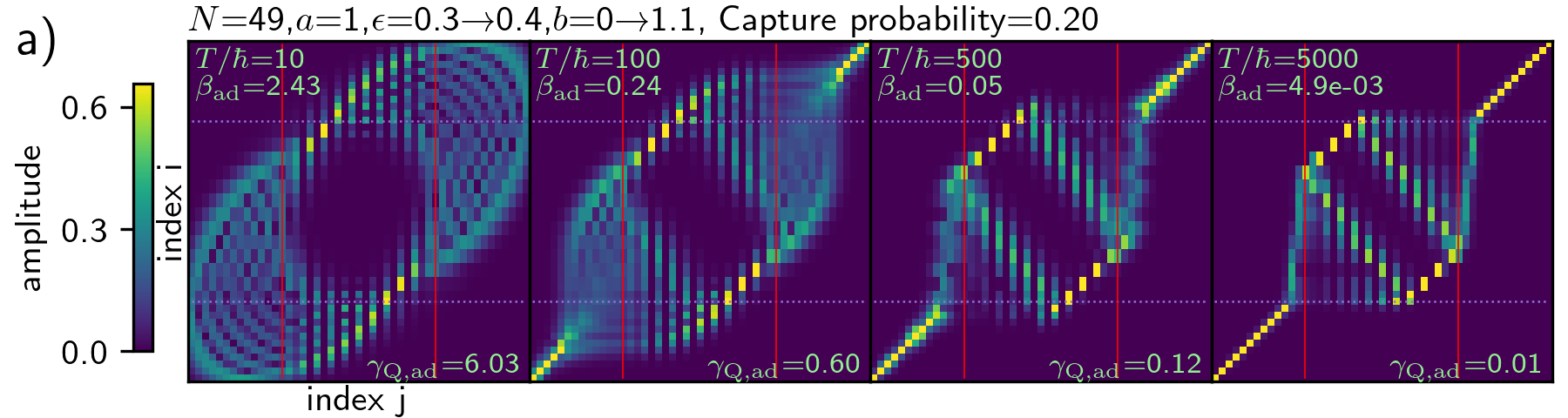
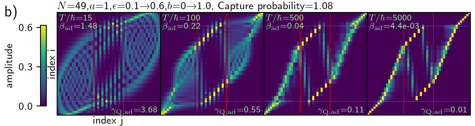
Figure 10: a) Similar to Figure 9a except we show transition matrices for the operator $\hat{h}(a,b(t),\epsilon(t)$ with both $b$ and $\epsilon$ varying. The probability of capture into the librating region is computed via equation 19 (via the KNH theorem) and is printed on the top of the image. For this series of integrations, the probability of capture is low. The dimensionless ratio $\beta_{\rm ad}$ which determines whether resonance capture is adiabatic for the associated classical system (computed via equation 15) is printed on each panel. The dimensionless ratio $\gamma_{Q,ad}$ (equation 20) describes whether drift is likely to cause Landau-Zener diabatic transitions in the librating regions is also printed on each panel. The red thin solid vertical lines are at the indices of the separatrices at the end of the simulation. The dotted thin horizontal purple lines are at the indices of initial location of the separatrices. b) Similar to a) except $\dot{\epsilon}$ and $\dot{b}$ are chosen so that the probability of capture into resonance is high.

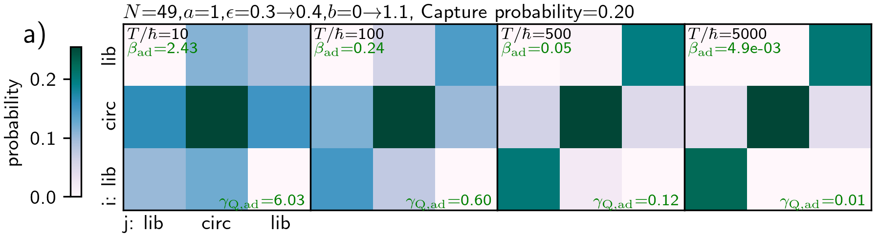
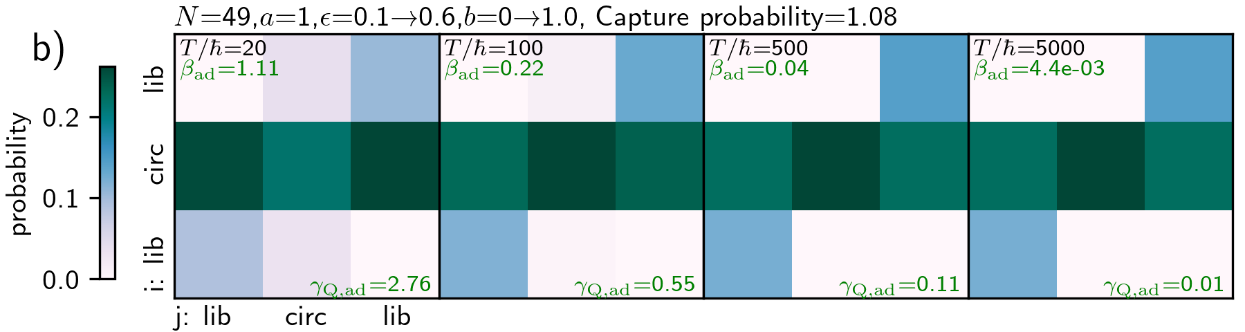
Figure 11: a) For the same integrations shown in Figure 10a, we show the probability of transition between an initial libration or circulation region and a final libration or circulation region. At slow drift rates (on the right) states begun in a librating region remain there and states begun in a circulating region remain there because the classically estimated probability of capture into resonance is low. At faster (and non-adiabatic) drift rates (on the left), transitions take place between states in circulating and librating regions. b) Similar to a) except for the integrations shown in Figure 10b. Because the resonance grows in width and the classically estimated probability of resonance capture is high, there are transitions between states initially in a circulating region and those in a librating region. At the two slowest drift rates (the right most two panels in a, and b)) the probabilities of transition between different regions are similar, indicating that drift is both classically adiabatic, $\beta_{\rm ad}<1$ and a quantum version of the KNH theorem holds (as shown by Stabel and Anglin [36]).

III.2 Varying both resonance strength and location

In this section we vary both resonance strength, set by $\epsilon$ and the $b$ parameter. We compare the transition matrix (equation 14) computed from the propagator (equation 13) that depends on the time dependent Hamiltonian $\hat{h}(a,b(t),\epsilon(t))$ at different drift rates. We compare the transition matrices for parameters that would give a low probability resonance capture in the associated classical system to one that would give a high probability of capture. A particle that starts in the circulating region and is later within a librating region is said to have been captured into resonance.

As shown by Henrard [21], Yoder [42] the probability of capture into resonance (provided drift is sufficiently adiabatic; $\beta_{\rm ad}\ll 1$) depends on a ratio of the rate that two volumes in phase space vary. For a pendulum with Hamiltonian $H(p,\phi)=a\frac{p^{2}}{2}-\epsilon\cos\phi$, the area within the resonance can be computed by integrating momentum inside the separatrix contour. At the separatrix energy $E_{sep}=a\frac{p^{2}}{2}-\epsilon\cos\phi=\epsilon$ giving $p(\phi)=\sqrt{\frac{2\epsilon}{a}}\sqrt{1+\cos\phi}$. The area within the separatrix orbit

$$V_{\rm res}=2\sqrt{\frac{2\epsilon}{a}}\int_{0}^{2\pi}\sqrt{1+\cos\phi}\ d\phi=16\sqrt{\frac{\epsilon}{a}}.$$ (17)

We use the pendulum to estimate the area inside the separatrix as it is much easier to integrate than the Harper model. The rate that the area of phase space within the resonance varies is

$$\dot{V}_{\rm res}=\frac{8\dot{\epsilon}}{\sqrt{\epsilon a}}=\frac{8\dot{\epsilon}}{\omega_{0}}.$$ (18)

The rate that the upper separatrix sweeps up volume in phase space, is $\dot{V}_{+}=2\pi\dot{b}$. The probability of capture into resonance (or capture into a libration region from a circulating region) based on the KNH theorem is

$$P_{c}\approx\frac{\dot{V}_{\rm res}}{\dot{V}_{+}}\approx\frac{\dot{\epsilon}}{\dot{b}}\frac{4}{\pi\sqrt{\epsilon a}}.$$ (19)

In Figure 10 we show transition matrices computed with both $\epsilon$ and $b$ varying linearly in time. The total distance in $b$ and $\epsilon$ that vary during the integration are shown on the top of each subfigure. The probability of capture, $P_{c}$, into the librating region is computed via equation 19 using the value of $\epsilon$ midway through the integration and is printed on the top of each plot. For Figure 10a, the ratio $\dot{b}/\dot{\epsilon}$ is sufficiently high that the probability of capture into the libration region is low. The opposite is true in Figure 10b where the probability of capture into the librating region is high. The dimensionless number $\beta_{\rm ad}$ (equation 15), characterizing whether the drift rate of the associated classical system would be considered adiabatic, is written on each panel.

Figure 10a the total drift in $b$ is about 1/3 of the distance across the $2\pi$ range for momentum $\hat{p}$. Because the probability of capture is low, most states that are initially within the circulation region remain in that region, to high probability, unless the drift rate is high. In Figure 10b, because the libration region grows in size, states initially in the circulating region are likely to transition into the librating region.

The dimensionless ratio $\Gamma$ of the Landau-Zener model is conceptually similar to the dimensionless parameter $\beta_{\rm ad}$ of equation 15. The dimensionless quantity $\beta_{\rm ad}$ is approximately the ratio of the time it takes the resonance to drift the distance of a resonance width and the libration period. The parameter $\Gamma$ is approximately the ratio of the time it takes to drift the eigenvalues a distance equal to the energy difference of the avoided crossing and the period of phase oscillations in the avoided crossing (which depends on the minimum energy difference and $\hbar$). Dimensionless ratios $\beta_{\rm ad}$ and $\Gamma$ are both likely to be important in a resonant quantum system, as $\beta_{\rm ad}\ll 1$ is required for transition probability integrated over different regions in phase space to match those predicted by the KNH theorem, whereas $\Gamma\ll 1$ is required for suppression of diabatic transitions between states.

We construct a dimensionless parameter in the spirit of the Landau-Zener model but dependent upon the energy level spacing in the bottom of the cosine potential well. For the Harper operator, the spacing between energy levels at the bottom of the potential well is $\Delta E=\hbar\omega_{0}$ with oscillation frequency $\omega_{0}=\sqrt{a\epsilon}$. The $\Gamma$ factor of the Landau-Zener model is the ratio of the square of an energy difference to $\hbar$ times an energy drift rate. It can be described as the ratio of the time to cross the energy difference at a specified energy drift rate and the period of phase oscillations caused by this energy difference. We construct a similar dimensionless quantity $\Gamma_{\rm ad}=\frac{(\hbar\omega_{0})^{2}}{\hbar\alpha}$ where $\alpha$ is an energy drift rate. If $b$ drifts by $2\pi$ then energy varies between its lowest and highest values, which for $|\epsilon/a|<1$ is a range of about 2a, giving $\alpha\sim{a\dot{b}}/{\pi}$. So that we have a parameter that is small when the system drifts adiabatically, we define a dimensionless ratio that is the inverse of $\Gamma_{\rm ad}$;

$$\gamma_{\rm Q,ad} =\Gamma_{\rm ad}^{-1}\sim\frac{\hbar a\dot{b}}{\pi(\hbar\omega_{0})^{2}}\sim\frac{1}{\pi\hbar\epsilon}\frac{\Delta b}{T}\sim\frac{N}{2\pi^{2}\epsilon}\frac{\Delta b}{T},$$ (20)

where we have used $\hbar=\frac{2\pi}{N}$ as the effective value of $\hbar$ for the quantized Harper operator [31]. The values of the dimensionless ratio $\gamma_{\rm Q,ad}$ are printed on each panel in Figure 10 a, b.

In Figure 10 we confirm that when $\gamma_{\rm Q,ad}\ll 1$ transitions between states in the librating region are unlikely. While $\gamma_{\rm Q,ad}$ is estimated using the energy spacing in the librating region, the difference in energy levels near the separatrix is only a few times smaller (see Figure 9b) than that in at the bottom of the potential well in the libration region. Thus $\gamma_{\rm Q,ad}$ can be used to estimate whether transitions are adiabatic or diabatic near the separatrices. As the probability of capture into resonance depends upon the nature of transitions in the vicinity of the separatrix, $\gamma_{\rm Q,ad}$ could give a quantum based estimate for whether transitions (or tunneling) would cause a deviation from the prediction of the KNH theorem.

Due to transitions into superposition states (also described as quantum tunneling), the classically estimated probability of capture into resonance (estimated via the KNH theorem) can underestimate the probability of capture into resonance. Stabel and Anglin [36] found that by summing over probabilities of Landau-Zener transitions, the KNH theorem could be modified to take into account both diabatic and adiabatic transition probabilities. In Figure 11 we compute the probabilities of transition between initial libration and circulation and final libration and circulation regions for the same integrations shown in Figure 10. The transition probabilities are estimated by summing the square of the transition matrix elements in regions of the transition matrix that are bounded by the indices of states with energies closest to those of the separatrix orbits. This Figure illustrates that a sum of transition probabilities between regions is sensitive to the drift rate, though as both $\beta_{\rm ad}$ and $\gamma_{\rm Q,ad}$ decrease as the drift rate decreases, it is difficult to separate between classical and quantum non-adiabatic behavior. We infer that the KNH theorem holds in the adiabatic limit of both $\beta_{\rm ad}\ll 1$ and $\gamma_{\rm Q,ad}\ll 1$ as the probabilities of transitions between regions of phase space approach values that are independent of drift rate in this limit. This inference is consistent with the picture described by Stabel and Anglin [36] generalizing the KNH theorem in the quantum setting. Note that even at the low drift rates on the right hand side of Figure 12 transitions between eigenstates take place within the circulation region where the energy levels are nearly degenerate. Thus the KNH is likely obeyed in the quantum system even when transitions into superposition states take place.

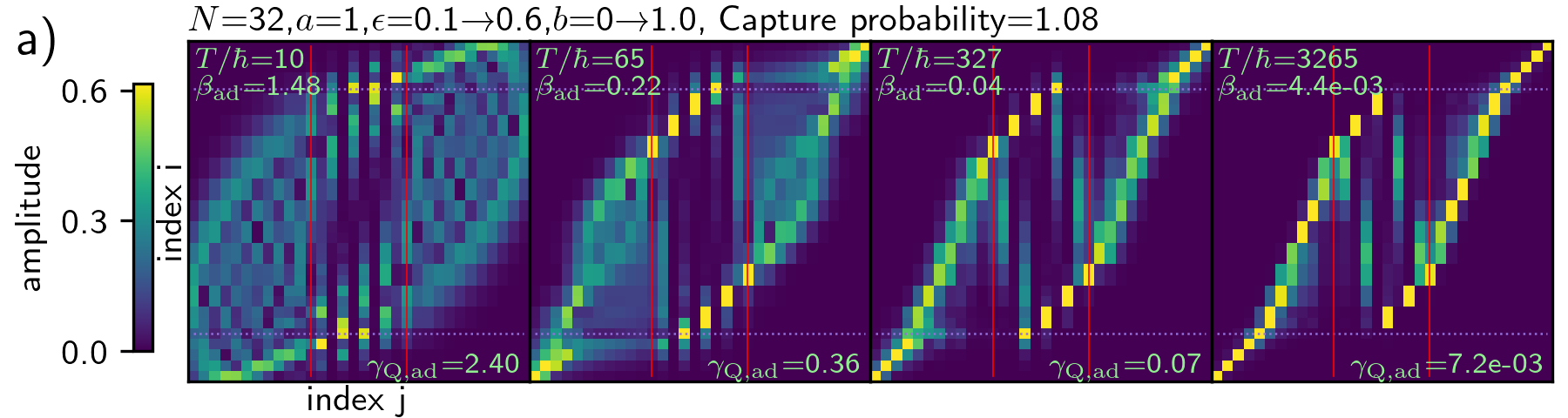
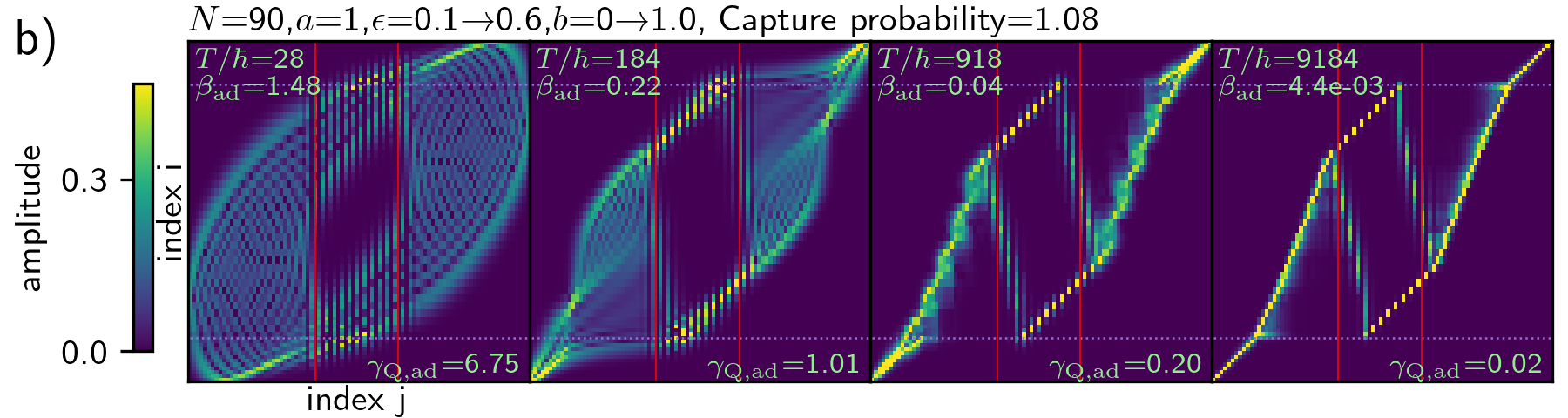
Figure 12: a) Similar to Figure 10b except the dimension of the quantum system $N=31$ differs and is lower than in Figure 10b. The durations $T$ of the drifts are the same as in Figure 10b. b) Similar to a) except $N=61$ is higher. Classical quantities $\beta_{\rm ad}$ (characterizing the adiabatic limit) and capture probability $P_{cap}$ are the same in a) and b) but because the effective value of $\hbar$ differs between the two operators, the parameter $\gamma_{\rm Q,ad}$, describing the likelihood of Landau-Zener transitions in the librating regions, differs between a) and b). The regions of phase space that undergo transitions are similar in the two models and governed by the classical adiabatic parameter $\beta_{\rm ad}$.

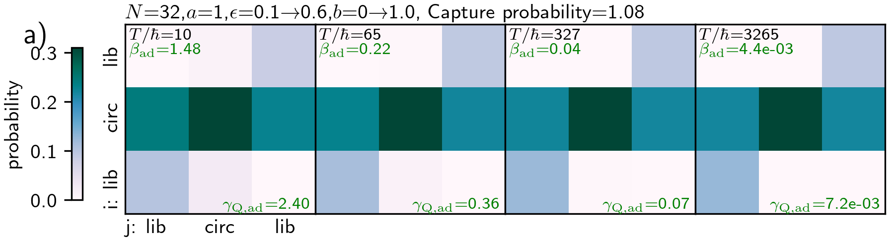
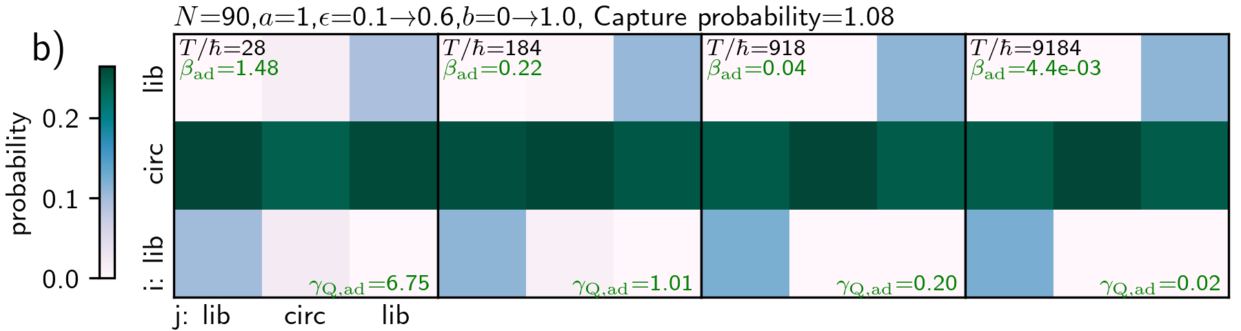
Figure 13: a) For the same integrations shown in Figure 12a, we show the probability of transition between an initial libration or circulation region and a final libration or circulation region. b) Similar to a) except for the integrations shown in Figure 12b.

Whereas dimensionless parameters $\beta_{\rm ad}$ (characterizing the adiabatic limit) and $P_{cap}$ (the probability of capture) are quantities describing the drifting classical model, $\gamma_{\rm Q,ad}$ depends on Planck’s constant $\hbar$. In Figure 12 we compare transition matrices for the same set of drift durations as shown in Figure 10b that has a high probability of capture into resonance, but with different dimensions $N$ and associated effective values of $\hbar$. Figure 12 shows that the probabilities of transitions between different regions of phase space is insensitive to drift rate as long as both $\gamma_{\rm Q,ad}\ll 1$ and $\beta_{\rm ad}\ll 1$. The transition matrices shown in Figure 12 have similar morphology at the two different $N$ values, so we attribute to the small differences in transition probabilities in Figure 12a, b to differences in the fraction of states in the different regions at low $N$.

The morphology of the transition matrices in Figure 12a, b are remarkably similar, so we suspect that the classical adiabatic parameter $\beta_{\rm ad}$ governs the probability of transitions between regions of phase space, though the Landau-Zener model would determine whether diabatic or adiabatic transitions take place between nearby (in energy) quantum states.

IV Summary and Discussion

The finite dimensional Harper operator is a simple quantum system on the phase space of a torus that exhibits complex behavior when time dependent. Even though it is remarkably simple when written in terms of shift and clock operators (see appendix A.1), and is related to an integrable (non-chaotic) classical system (see Figure 1), the notion of adiabatic drift is non-trivial in the quantum system because of the presence of separatrix orbits in the associated classical system that divide phase space into librating and circulating regions. Because the operator is finite dimensional, it is straight forward to numerically evaluate its spectrum and because it is simply written in terms of operators, a number of symmetries can be exploited to aid in studying its spectrum (see appendix A).

We find that the nature of spectrum of the quantized system depends upon whether eigenstate energies are in the circulating or librating region of the associated classical system. Within the librating region, energy levels are well separated, however, in the circulating region, pairs of eigenvalues are nearly degenerate. When the center of the resonance is drifted, via increasing or decreasing the $b$ parameter which sets the center of resonance, the spectrum in the circulating region exhibits a lattice of avoided energy level crossings (Figures 3, and 4). In the librating region, the energy levels are shifted and the spacing varies to a lesser extent. The difference in behavior is explained heuristically in section II.2 with a perturber harmonic oscillator (for the librating region) and rotor (for the circulating region). Symmetries of the Harper operator imply that near degeneracies in the spectrum occur at $b$ multiples of $\pi/N$ (see appendixes A.2, A.3, A.6 and Figure 3).

Despite the simplicity of the Harper operator, it exhibits an extremely wide range in its energy level spacings which affects evolution of the quantum system when the Hamiltonian operator is time dependent. For parameter $b$ (which sets the resonance center) slowly varying, the energy levels of eigenstates in the librating region are not much affected, however energy levels within the circulating region undergo a series of close approaches with minimum distance between pairs of eigenvalues that span many orders of magnitude (e.g., see Figure 7). The minimum spacing is in the middle of circulating region and depends on a high power of the resonance strength parameter (equation 8, appendix LABEL:ap:min_spacing). This high power would be difficult to predict with conventional perturbation theory. We computed the propagator of the time dependent Hamiltonian operator for systems that vary the same total amount in $b$ but over different durations. For a quantum state initialized in an eigenstate, transitions take place over a wide range in drift rates (see Figure 9). Only at drift rates many orders of magnitude below the classical adiabatic limit for resonance capture would a system initially begun in any eigenstate remain in one.

In quantum systems, one notion of adiabatic drift is that drift is sufficiently slow that a system initialized in an eigenstate state of a time dependent Hamiltonian operator would remain in an eigenstate of the Hamiltonian. This notion is consistent with the two level Landau-Zener model. In this sense, only at negligible drift rates would the time dependent Harper operator behave adiabatically for all possible initial conditions. This is not inconsistent with the fact pointed out by Berry and Robnik [3]; adiabatic and semiclassical limits give opposite results when two levels in a slowly-changing system pass a near-degeneracy.

In a classical system containing a separatrix orbit, an alternate notion of adiabatic behavior is whether the probability for resonance capture is well described by a probability computed via the KNH theorem which is based on conservation of volume in phase space (Liouville’s theorem). At sufficiently slow drift rates, by taking account all transition probabilities, Stabel and Anglin [36] showed using a semi-classical limit that a quantum system approaches the same resonance capture probability as predicted from the KNH theorem. We support, confirm and expand on the work by Stabel and Anglin [36] with a complimentary and finite dimensional Hamiltonian model. A classical drifting resonance can be described via two dimensionless parameters, a capture probability (computed via the KNH theorem) and a dimensionless parameter that describes whether the drift is sufficiently slowly that it is considered adiabatic (the $\beta_{\rm ad}$ parameter of equation 15). For a resonant quantum system we estimate an additional dimensionless parameter $\gamma_{\rm Q,ad}$ (equation 20), similar to the $\Gamma$ parameter of the Landau-Zener model, to describe whether states in the resonance libration region are sufficiently separated (in energy) that the drift rate would not cause diabatic transitions near the separatrix energy. We find that probabilities of transition between different regions of phase space seems primarily dependent upon the classical parameter, with probability approaching a constant value for $\beta_{\rm ad}\ll 1$. However, transitions in the vicinity of the separatrix cease for $\gamma_{\rm Q,ad}\ll 1$. Because of the wide range in energy level spacings that are present in a quantized system associated with a classical one that contains a separatrix orbit, transitions between eigenstates take place in the circulation region even if the drift rate is sufficiently slow that the KNH theorem should hold. In other words, drift can be sufficiently adiabatic that the KNH theorem would be obeyed in a quantum system, taking into account multiple transitions near the separatrix region. Yet a system begun in a eigenstate would not necessarily remain in one particularly if there is a large range in separations between neighboring eigenvalues. The notion of adiabatic behavior in which both quantized and classical systems obey the KNH theorem for resonance capture is consistent with but differs from the notion of adiabatic behavior in which a system begun in an eigenstate remains in an eigenstate of a time dependent Hamiltonian operator. In the vicinity of a separatrix in a classical system, the dynamics is not strictly adiabatic. The associated quantum manifestation of non-adiabatic behavior near the separatrix energy could be the existence of diabatic transitions.

Expansion of a non-local or long range perturbation, such as the gravitational force from a planet, gives a series of cosine terms, each associated with an orbital resonance (e.q., [30]). Hence cosine potential terms are ubiquitous in many complex classical Hamiltonian systems. Many of the symmetries obeyed by the quantized Harper model would also be obeyed by finite dimensional quantum operators with additional Fourier terms (see appendix LABEL:ap:other). There is similarity between the spectrum of the finite dimensional Harper operator and the Mathieu equation (appendix LABEL:ap:mathieu). This implies that the finite dimensional Harper model and its variants could be used to approximate infinite dimensional quantum systems with cosine or more complex non-local potentials. Future studies could attempt to determine if there is a type of universality associated with resonant quantum systems that is illustrated via the deceptively simple looking Harper operator.

The quantum pendulum has nearly degenerate eigenvalues with spacing that decreases as index $m\to\infty$. Consequently for any drift rate, no matter how slow, there would be some energy above which diabatic transitions would occur (see appendix LABEL:ap:mathieu). Despite the fact that the distance between pairs of energy levels increases with energy ($\propto m^{2}$ with eigenstate index $m$), the energy difference between the states in each pair shrinks rapidly. The difference drops so rapidly (via a power law) that near degeneracy can be reached at a moderate energy. In this sense, it is amusing to think of the the quantized pendulum as an example of a quantum system that has no formal adiabatic limit. An implication is that if ionization (or transitions to the circulating region) can occur (e.g., in transmons [18]) then non-adiabatic phenomena could be present over a wide range of possible drift or driving frequencies.

While there are a number of techniques for placing limits on eigenvalues of an operator using perturbation theory or with the Cauchy interlacing theorem or Weyl’s inequalities, (e.g., [28, 4]), it is more challenging to place limits on the spacing between eigenvalues (though see [23, 20, 26, 43]). This motivates studying specific systems, such as the Harper model, which could represent a class of resonant models, and for developing additional tools in linear algebra to aid in estimating distances between eigenvalues.

Adiabatic and diabatic phenomena are relevant for design of counter-diabadic protocols or transitionless quantum driving [14, 10, 34], and adiabatic computational algorithms. Design of varying Hamiltonians that purposely contain a range of gap sizes could be used for the opposite effect, giving enhanced numbers of transitions for fast effective thermalization. The system we have studied here is based on an integrable classical system, and more complex phenomena is likely to be present in drifting systems that are associated with chaotic classical systems (e.g., [31]).

Acknowledgements

We thank Sreedev Manikoth for helpful discussions.

Figures in this manuscript are generated with python notebooks available at https://github.com/aquillen/H0drift.

Appendix A Properties of the spectrum of the Harper operator

A.1 The discrete and shifted Harper/finite almost Mathieu operator

Our quantum space is an $N$ dimensional complex vector space, typically with $N>3$. In an orthonormal basis denoted $\{\ket{j}\}:j\in\{0,1,\ldots,N-1\}$, the discrete Fourier transform is

$$\hat{Q}_{FT} =\frac{1}{\sqrt{N}}\sum_{j,k=0}^{N-1}\omega^{jk}\ket{j}\bra{k},$$ (21)

with complex root of unity

$$\omega \equiv e^{2\pi i/N}.$$ (22)

Using the discrete Fourier transform, we construct an orthonormal basis consisting of states

$$\ket{m}_{F}=\hat{Q}_{FT}\ket{m}=\frac{1}{\sqrt{N}}\sum_{j=0}^{N-1}\omega^{mj}\ket{j}$$ (23)

with $m\in\{0,1,\ldots,N-1\}$.

Angle and momentum operators are defined using the conventional and Fourier bases (defined in equation 23),

$$\hat{\phi} =\sum_{j=0}^{N-1}\frac{2\pi j}{N}\ket{j}\bra{j}$$

$$\hat{p} =\sum_{k=0}^{N-1}\frac{2\pi k}{N}\ket{k}_{F}\bra{k}_{F}.$$ (24)

Clock and shift operators [33] are defined as

$$\hat{Z} =\sum_{j=0}^{N-1}\omega^{j}\ket{j}\bra{j}=\sum_{k=0}^{N-1}\ket{(k+1)\text{ mod }N}_{F}\bra{k}_{F}$$

$$\hat{X} =\sum_{k=0}^{N-1}\omega^{-k}\ket{k}_{F}\bra{k}_{F}=\sum_{j=0}^{N-1}\ket{(j+1)\text{ mod }N}\bra{j}.$$ (25)

The clock and shift operators are also called generalized Pauli matrices or Weyl-Heisenberg matrices [2]. They obey

$$\hat{Z}\hat{X} =\omega\hat{X}\hat{Z},\qquad\hat{Z}\hat{X}^{\dagger}=\omega^{-1}\hat{X}^{\dagger}\hat{Z}$$ (26)

and

$$\hat{Z} =\hat{Q}_{FT}\hat{X}\hat{Q}_{FT}^{\dagger},\qquad\hat{Z}^{\dagger}=\hat{Q}_{FT}^{\dagger}\hat{X}\hat{Q}_{FT}$$

$$\hat{Z}^{N} =\hat{X}^{N}=\hat{I}$$ (27)

where $\hat{I}$ is the identity operator.

The parity operator

$$\hat{P}=\sum_{n=0}^{N-1}\ket{n}\bra{-n\ {\rm mod}\ N}=\sum_{k=0}^{N-1}\ket{k}_{F}\bra{-k\ {\rm mod}\ N}_{F}.$$ (28)

Trigonometric functions are particularly simple in terms of the clock and shift operators,

$$\cos\hat{\phi} =\frac{1}{2}(\hat{Z}+\hat{Z}^{\dagger})$$

$$\sin\hat{\phi} =\frac{1}{2i}(\hat{Z}-\hat{Z}^{\dagger})$$

$$\cos\hat{p} =\frac{1}{2}(\hat{X}+\hat{X}^{\dagger})$$

$$\sin\hat{p} =\frac{1}{2i}(-\hat{X}+\hat{X}^{\dagger}).$$ (29)

We are interested in the spectrum and the dynamics of the $N$-dimensional Hermitian operator of equation 6 which we restate here,

$$\hat{h}\left(a,b,\epsilon\right) =a\cos(\hat{p}-b)+\epsilon\cos\hat{\phi},$$ (30)

and with $\hat{p},\hat{\phi}$ operators defined in equation 24. The coefficients $a,\epsilon,b$ are real numbers, and typically $a>0$ and $|\epsilon|\leq 1$. With $b=0$, this operator is equivalent to the finite almost Mathieu operator studied by Strohmer and Wertz [37]. The parameter $b$ allows us to shift the momentum or kinetic operator term as illustrated for the classical system in Figure 1. Except for its sign and a constant term proportional to the identity operator, the operator $\hat{h}$ is similar to the operator we studied previously [31] (called $\hat{h}_{0}$) that was derived from the classical Harper Hamiltonian [19]. The operator is traceless $\tr\hat{h}(a,b,\epsilon)=0$.

In terms of clock and shift operators, the Hermitian operator of equation 30

$$\hat{h}\left(a,b,\epsilon\right) =\frac{a}{2}\left(\hat{X}+\hat{X}^{\dagger}\right)\cos b+\frac{a}{2i}\left(-\hat{X}+\hat{X}^{\dagger}\right)\sin b$$

$$\ \ \ \ +\frac{\epsilon}{2}\left(\hat{Z}+\hat{Z}^{\dagger}\right)$$

$$=\frac{a}{2}\hat{X}e^{ib}+\frac{a}{2}\hat{X}^{\dagger}e^{-ib}+\frac{\epsilon}{2}\left(\hat{Z}+\hat{Z}^{\dagger}\right).$$ (31)

With $b=0$, $a=\epsilon$, the operator commutes with the discrete Fourier transform operator,

$$\left[\hat{Q}_{FT},\hat{h}\left(a,0,a\right)\right]=0$$ (32)

so the finite almost Mathieu operator helps classify eigenstates of the discrete Fourier transform [15].

The Hermitian operator $\hat{h}$ is triagonal with the addition of two additional terms on the top right and lower left corners and in the form

$$\begin{pmatrix}\alpha_{0}&\beta^{*}&0&\cdots&0&\beta\\ \beta&\alpha_{1}&\beta^{*}&\ddots&\vdots&0\\ 0&\beta&\alpha_{2}&\ddots&\vdots&\vdots\\ \vdots&\ddots&\ddots&\ddots&\ddots&\vdots\\ 0&\cdots&\ddots&\beta&\alpha_{N\!-\!2}&\beta^{*}\\ \beta^{*}&0&\cdots&0&\beta&\alpha_{N\!-\!1}\end{pmatrix}.$$ (33)

In the conventional basis and for $j\in\{0,1,\ldots,N-1\}$, the operator $\hat{h}(a,b,\epsilon)$ is a Hermitian matrix in the form of 33 with coefficients

$$\alpha_{j} =\epsilon\cos\left(\frac{2\pi j}{N}\right)$$

$$\beta =\frac{a}{2}e^{ib}.$$ (34)

In the Fourier basis (defined in equation 23) and for $k\in\{0,1,\ldots,N-1\}$, the operator $\hat{h}(a,b,\epsilon)$ is a symmetric real matrix in the form of 33 with coefficients

$$\alpha_{k} =a\cos\left(\frac{2\pi k-b}{N}\right)$$

$$\beta =\frac{\epsilon}{2}.$$ (35)

A.2 How shifts in parameter $b$ affect the spectrum

From shift, clock and parity operators, we can try to construct an invertible operator $\hat{V}$ that obeys $\hat{V}\hat{h}(a,b,\epsilon)\hat{V}^{-1}=\hat{h}(a^{\prime},b,^{\prime}\epsilon^{\prime})$ where $a^{\prime},b^{\prime},\epsilon^{\prime}$ are not necessarily the same parameters as $a,b,\epsilon$. If we can find such an operator $\hat{V}$, then the spectrum of $h(a,b,\epsilon)$ is the same as the spectrum of $\hat{h}(a^{\prime},b^{\prime},\epsilon^{\prime})$.

Theorem A.1.

For the operator $\hat{h}(a,b,\epsilon)$ in equation 30 and $k\in{\mathbb{Z}}$, the spectrum or set of eigenvalues obeys

$${\rm spectrum}\left[\hat{h}\left(a,\dfrac{2\pi k}{N},\epsilon\right)\right] ={\rm spectrum}\left[\hat{h}\left(a,0,\epsilon\right)\right].$$ (36)

Proof.

We use short-hand $e^{\frac{2\pi ik}{N}}=\omega^{k},$ and equation 31 to find

$$\hat{h}(a,\frac{2\pi k}{N},\epsilon) =\frac{a}{2}\hat{X}\omega^{k}+\frac{a}{2}\hat{X}^{\dagger}\omega^{-k}+\frac{\epsilon}{2}\left(\hat{Z}+\hat{Z}^{\dagger}\right).$$ (37)

For $k\in{\mathbb{Z}}$, using the relations in equations 26

$$\hat{Z}^{k}\hat{X}\hat{Z}^{-k} =\omega^{k}\hat{X}$$

$$\hat{Z}^{k}\hat{X}^{\dagger}\hat{Z}^{-k} =\omega^{-k}\hat{X}^{\dagger}.$$ (38)

These relations help us compute

$$\hat{Z}^{-k}\hat{h}\left(a,\frac{2\pi k}{N},\epsilon\right)\hat{Z}^{k}=\hat{h}\left(a,0,\epsilon\right).$$ (39)

The operator $\hat{h}$ is Hermitian, and so it is diagonalizable. Since $\hat{Z}^{k}$ is an invertible operator (that is also unitary), equation 39 implies that the two operators in equation 39 have the same set of eigenvalues or spectrum. ∎

Corollary A.2.

If $\ket{n}$ is an eigenstate of $\hat{h}(a,0,\epsilon)$ with eigenvalue $\lambda_{n}$, then for $k\in{\mathbb{Z}}$, $Z^{k}\ket{n}$ is an eigenstate of $\hat{h}(a,\frac{2\pi k}{N},\epsilon)$ with the same eigenvalue.

Proof.

Using equation 39

$$\hat{Z}^{-k}\hat{h}\left(a,\frac{2\pi k}{N},\epsilon\right)\hat{Z}^{k}\ket{n} =\hat{h}\left(a,0,\epsilon\right)\ket{n}=\lambda_{n}\ket{n}$$

$$\hat{h}\left(a,\dfrac{2\pi k}{N},\epsilon\right)\hat{Z}^{k}\ket{n} =\lambda_{n}\hat{Z}^{k}\ket{n}.$$ (40)

This implies that $\lambda_{n}$ is an eigenvalue of $\hat{h}(a,\frac{2\pi k}{N},\epsilon)$ with eigenstate $\hat{Z}^{k}\ket{n}$. ∎

Theorem A.3.

For the operator $\hat{h}(a,b,\epsilon)$ defined in equation 30, $k\in{\mathbb{Z}}$, and $0\leq r<\frac{2\pi}{N}$,

$${\rm spectrum}\left[\hat{h}\left(a,r+\dfrac{2\pi k}{N},\epsilon\right)\right] ={\rm spectrum}\left[\hat{h}\left(a,r,\epsilon\right)\right].$$ (41)

Proof.

Equation 31 and equations 38 give

$$\hat{Z}^{-k}\hat{h}\left(a,\dfrac{2\pi k}{N}+r,\epsilon\right)\hat{Z}^{k} =\frac{a}{2}\left(\hat{X}\omega^{r}+\hat{X}^{\dagger}\omega^{-r}\right)+\epsilon\cos\hat{\phi}$$

$$=\hat{h}\left(a,r,\epsilon\right).$$ (42)

As $Z^{k}$ is a unitary operator which is invertible, this implies that both operators in equation 42 have the same spectrum. ∎

Corollary A.4.

With $0\leq r<\frac{2\pi}{N}$, if $\ket{n}$ is an eigenstate of $\hat{h}(a,r,\epsilon)$ with with eigenvalue $\lambda_{n}$, then $Z^{k}\ket{n}$ is an eigenstate of $\hat{h}(a,r+\frac{2\pi k}{N},\epsilon)$ with the same eigenvalue.

This corollary follows directly from equation 42.

Theorem A.5.

For $\hat{h}$ defined in equation 30

$${\rm spectrum}\left[\hat{h}(a,b,\epsilon)\right] ={\rm spectrum}\left[\hat{h}(a,-b,\epsilon)\right].$$ (43)

Proof.

With parity operator $\hat{P}$ defined in equation 28 we find that

$$\hat{P}\hat{Z}\hat{P} =\hat{Z}^{\dagger}$$

$$\hat{P}\hat{X}\hat{P} =\hat{X}^{\dagger}.$$ (44)

This implies that

$$\hat{P}\cos\hat{p}\ \hat{P} =\cos\hat{p}$$

$$\hat{P}\cos\hat{\phi}\ \hat{P} =\cos\hat{\phi}$$

$$\hat{P}\sin\hat{p}\ \hat{P} =-\sin\hat{p}$$

$$\hat{P}\sin\hat{\phi}\ \hat{P} =-\sin\hat{\phi}$$ (45)

As the parity operator commutes with both $\cos\hat{p}$ and $\cos\hat{\phi}$, when $b=0$, the Hamiltonian operator $\hat{h}$ commutes with the parity operator

$$\left[\hat{P},\hat{h}(a,0,\epsilon)\right]=0.$$ (46)

For $b\neq 0$

$$\hat{P}\hat{h}(a,b,\epsilon)\hat{P} =a\cos\hat{p}\cos b-a\sin\hat{p}\sin b+\epsilon\hat{\cos}\phi$$

$$=\hat{h}(a,-b,\epsilon).$$ (47)

Because the parity operator $\hat{P}$ is its own inverse, equation 47 implies that the two operators in equation 47 have the same spectrum. ∎

Corollary A.6.

For $k\in{\mathbb{Z}}$, and $0\leq r<\frac{2\pi}{N}$

$${\rm spectrum}\left[\hat{h}\left(a,r+\frac{2\pi}{N},\epsilon\right)\right] ={\rm spectrum}\left[\hat{h}(a,\pm r,\epsilon)\right].$$ (48)

Proof.

A consecutive use of theorems A.5 and A.3 together imply that the two operators in equation 48 have the same spectrum. ∎

Corollary A.7.

For $\ket{n}$ an eigenstate of $\hat{h}(a,b,\epsilon)$ (defined in equation 30), the state $\hat{P}\ket{n}$ (where $\hat{P}$ is the parity operator) is an eigenstate of $\hat{h}(a,-b,\epsilon)$ with the same eigenvalue.

Proof.

We take $\ket{n}$ to be an eigenstate of $\hat{h}(a,b,\epsilon)$ with eigenvalue $\lambda_{n}$. Using equation 47

$$\hat{P}\hat{h}(a,-b,\epsilon)\hat{P}\ket{n} =\hat{h}(a,b,\epsilon)\ket{n}=\lambda_{n}\ket{n}$$

$$\hat{h}(a,-b,\epsilon)\hat{P}\ket{n} =\lambda_{n}\hat{P}\ket{n}.$$

This implies that $\hat{P}\ket{n}$ is an eigenstate of $\hat{h}(a,-b,\epsilon)$ with the same eigenvalue $\lambda_{n}$. ∎

Theorem A.8.

For $k\in{\mathbb{Z}}$, remainder $0\leq\delta<\frac{\pi}{N}$ and operator $\hat{h}$ defined in equation 30

$${\rm spectrum}\left[\hat{h}\left(a,\frac{(2k+1)\pi}{N}+\delta,\epsilon\right)\right]=\qquad\qquad\ \$$

$$\qquad{\rm spectrum}\left[\hat{h}\left(a,\frac{\pi}{N}-\delta,\epsilon\right)\right].$$ (49)

Proof.

With a calculation similar to equation 42, we find that

$$\hat{Z}^{\dagger}\hat{h}\left(a,\frac{\pi}{N}+\delta,\epsilon\right)\hat{Z} =\hat{h}\left(a,-\frac{\pi}{N}+\delta,\epsilon\right).$$ (50)

Applying the parity operator

$$\hat{P}\hat{Z}^{\dagger}\hat{h}\left(a,\frac{\pi}{N}+\delta,\epsilon\right)\hat{Z}\hat{P} =\hat{h}\left(a,\frac{\pi}{N}-\delta,\epsilon\right).$$ (51)

The product $\hat{Z}\hat{P}$ is invertible with inverse $\hat{P}\hat{Z}^{\dagger}$ as $\hat{Z}$ is unitary and $\hat{P}$ is its own inverse, so equation 51 implies that the two operators have the same spectrum. We then apply theorem A.3 to show that the spectra of the two operators in equation 49 are equivalent. ∎

Corollary A.9.

$$\left[\hat{P}\hat{Z}^{\dagger},\hat{h}(a,\frac{\pi}{N},\epsilon)\right]=0.$$ (52)

Proof.

Equation 52 follows directly from equation 51 using $\delta=0$.

∎

Corollary A.10.

If $\ket{n}$ is an eigenstate of $\hat{h}(a,\frac{\pi}{N}+\delta,\epsilon)$ with eigenvalue $\lambda_{n}$, then $\hat{P}\hat{Z}^{\dagger}\ket{n}$ is an eigenstate of $\hat{h}(a,\frac{\pi}{N}-\delta,\epsilon)$ with the same eigenvalue.

Proof.

Using equation 51

$$\hat{Z}\hat{P}\hat{h}\left(a,\frac{\pi}{N}-\delta,\epsilon\right)\hat{P}\hat{Z}^{\dagger} =\hat{h}\left(a,\frac{\pi}{N}+\delta,\epsilon\right)$$

$$\hat{Z}\hat{P}\hat{h}\left(a,\frac{\pi}{N}-\delta,\epsilon\right)\hat{P}\hat{Z}^{\dagger}\ket{n} =\lambda_{n}\ket{n}$$

$$\hat{h}\left(a,\frac{\pi}{N}-\delta,\epsilon\right)\hat{P}\hat{Z}^{\dagger}\ket{n} =\lambda_{n}\hat{P}\hat{Z}^{\dagger}\ket{n}.$$ (53)

This shows that $\hat{P}\hat{Z}^{\dagger}\ket{n}$ is an eigenstate of $\hat{h}\left(a,\frac{\pi}{N}-\delta,\epsilon\right)$ with eigenvalue $\lambda_{n}$. ∎

Theorem A.11.

for $k\in\mathbb{Z}$,

$$\left[\hat{P}\hat{Z}^{-2k},\hat{h}\left(a,\frac{2\pi k}{N},\epsilon\right)\right]=0.$$ (54)

Proof.

Equation 39 gives

$$\hat{Z}^{-k}h\left(a,\frac{2\pi k}{N},\epsilon\right)\hat{Z}^{k}=\hat{h}(a,0,\epsilon).$$ (55)

We use the fact that parity $\hat{P}$ commutes with $\hat{h}(a,0,\epsilon)$ (equation 46) giving

$$\hat{P}\hat{Z}^{-k}h\left(a,\frac{2\pi k}{N},\epsilon\right)\hat{Z}^{k}\hat{P} =\hat{h}(a,0,\epsilon)$$

$$=\hat{Z}^{-k}\hat{h}\left(a,\frac{2\pi k}{N},\epsilon\right)\hat{Z}^{k}$$ (56)

and

$$\hat{Z}^{k}\hat{P}Z^{-k}h\left(a,\frac{2\pi k}{N},\epsilon\right)\hat{Z}^{k}\hat{P}\hat{Z}^{-k} =\hat{h}\left(a,\frac{2\pi k}{N},\epsilon\right).$$ (57)

We use the fact that $\hat{P}\hat{Z}=\hat{Z}^{\dagger}\hat{P}$ (from equation 44) to give

$$\hat{P}Z^{-2k}h\left(a,\frac{2\pi k}{N},\epsilon\right)\hat{Z}^{2k}\hat{P} =\hat{h}\left(a,\frac{2\pi k}{N},\epsilon\right)$$ (58)

which gives the commutator of equation 54. ∎

This symmetry is related to the close approaches between eigenvalues at $b$ a multiple of $2\pi/N$.

Theorem A.12.

For $k\in\mathbb{Z}$,

$$\left[\hat{P}\hat{Z}^{-(2k+1)},\hat{h}\left(a,\frac{\pi(2k+1)}{N},\epsilon\right)\right]=0.$$ (59)

Proof.

Using equation 42 with $r=\frac{\pi}{N}$ and with $k\in\mathbb{Z}$

$$\hat{Z}^{-k}\hat{h}\left(a,\frac{\pi(2k+1)}{N},\epsilon\right)\hat{Z}^{k} =\hat{h}\left(a,\frac{\pi}{N},\epsilon\right).$$ (60)

Using Equation 52

$$\hat{P}\hat{Z}^{-(k+1)}\hat{h}\Big{(}a, \frac{\pi(2k+1)}{N},\epsilon\Big{)}\hat{Z}^{k+1}\hat{P}=\hat{h}\left(a,\frac{\pi}{N},\epsilon\right)$$

$$=\hat{Z}^{-k}\hat{h}\left(a,\frac{\pi(2k+1)}{N},\epsilon\right)\hat{Z}^{k}.$$ (61)

We multiply both sizes by factors of $\hat{Z}$,

$$Z^{k}\hat{P}\hat{Z}^{-(k\!+\!1)}\hat{h}\left(a,\!\frac{\pi(2k\!+\!1)}{N},\epsilon\right) \hat{Z}^{k\!+\!1}\hat{P}\hat{Z}^{-k}$$

$$\!=\hat{h}\left(a,\!\frac{\pi(2k\!+\!1)}{N},\epsilon\right).$$

We commute the parity operator

$$\hat{P}\hat{Z}^{-(2k+1)}\hat{h}\left(a,\!\frac{\pi(2k\!+\!1)}{N},\epsilon\right)\hat{Z}^{2k\!+\!1}\hat{P} =\hat{h}\left(a,\frac{\pi(2k\!+\!1)}{N},\epsilon\right)$$ (62)

and this gives the commutator in equation 59. ∎

This symmetry is related to the close approaches between eigenvalues at $b$ at odd multiples of $\pi/N$.

Theorem A.13.

The spectrum of $\hat{h}(a,0,\epsilon)$ is the same as the spectrum of $\hat{h}(\epsilon,0,a)$.

Proof.

We apply the discrete Fourier transform (equation 27), giving

$$\hat{Q}_{FT}\hat{h}(a,0,\epsilon)\hat{Q}_{FT}^{-1}=\hat{h}(\epsilon,0,a).$$ (63)

This implies that the spectrum of $\hat{h}(a,0,\epsilon)$ is the same as that of $\hat{h}(\epsilon,0,a)$. ∎

A.3 The derivatives of the eigenvalues with respect to drift parameter $b$

We consider how the eigenvalues of $\hat{h}(a,b,\epsilon)$ (defined in equation 30) vary when $b$ varies. We take $\ket{n(b)}$ to be an eigenstate that satisfies $\hat{h}(a,b,\epsilon)\ket{n(b)}=\lambda_{n}(b)\ket{n(b)}$ with eigenvalue $\lambda_{n}(b)$.

Theorem A.14.

For $k\in{\mathbb{Z}}$, each eigenvalue $\lambda_{n}(b)$ of $\hat{h}(a,b,\epsilon)$ (defined in equation 30) that remains distinct from other eigenvalues obeys

$$\frac{\partial}{\partial b}\lambda_{n}(b)\Bigg{|}_{b=\frac{k\pi}{N}}=0.$$ (64)

Proof.

Using equation 31

$$\frac{\partial}{\partial b}\hat{h}(a,b,\epsilon) =a\sin(\hat{p}-b)$$ (65)

$$\frac{\partial}{\partial b}h(a,b,\epsilon)\Bigg{|}_{b=0} =a\sin\hat{p}.$$ (66)

We apply the Hellman-Feynman theorem (e.g., [35]) which gives the expression

$$\bra{n(b)}\frac{\partial}{\partial b}\hat{h}(a,b,\epsilon)\ket{n(b)} =\frac{\partial}{\partial b}\lambda_{n}(b).$$ (67)

At $b=0$

$$\bra{n(0)}\frac{\partial}{\partial b}\hat{h}(a,b,\epsilon)\Bigg{|}_{b=0}\ket{n(0)} =\frac{\partial}{\partial b}\lambda_{n}(b)\Bigg{|}_{b=0}.$$ (68)

Using equation 66

$$\bra{n(0)}a\sin\hat{p}\ket{n(0)}=\frac{\partial}{\partial b}\lambda_{n}(b)\Bigg{|}_{b=0}.$$ (69)

We previously showed (equation 46) that for $b=0$, $\hat{h}$ commutes with the parity operator $\hat{P}$. Hence an eigenstate with a distinct eigenvalue must also be an eigenstate of the parity operator which has eigenvalues of $\pm 1$. That implies that

$$\bra{n(0)}\hat{P}a\sin\hat{p}\hat{P}\ket{n(0)}=\bra{n(0)}a\sin\hat{p}\ket{n(0)}.$$ (70)

However we also showed previously that $\hat{P}\sin\hat{p}\hat{P}=-\sin\hat{p}$ (equation 45). This implies that

$$\bra{n(0)}\hat{P}a\sin\hat{p}\hat{P}\ket{n(0)}=-\bra{n(0)}a\sin\hat{p}\ket{n(0)}$$ (71)

Together these imply that

$$\bra{n(0)}a\sin\hat{p}\ket{n(0)}=-\bra{n(0)}a\sin\hat{p}\ket{n(0)}=0.$$ (72)

Hence equation 69 gives

$$\frac{\partial}{\partial b}\lambda_{n}(b)\Bigg{|}_{b=0}=0.$$ (73)

We extend this to $b$ a multiple of $2\pi/N$ using theorem A.3.

It is convenient to compute

$$\hat{Z}\sin(\hat{p}-b)\hat{Z}^{\dagger} =\sin(\hat{p}+\frac{2\pi}{N}-b).$$ (74)

We find that $\hat{P}\hat{Z}^{\dagger}$ commutes with $\hat{h}(a,\frac{\pi}{N},\epsilon)$ which means $\hat{P}\hat{Z}^{\dagger}$ and $\hat{h}(a,\frac{\pi}{N},\epsilon)$ are simultaneously diagonalizable. Because $\hat{P}\hat{Z}^{\dagger}$ is a unitary operator, its eigenvalues are complex numbers with magnitude 1 so they cancel in the following expression

$$\bra{n}\hat{Z}\hat{P}\sin(\hat{p}+\frac{\pi}{N})\hat{P}\hat{Z}^{\dagger}\ket{n} =\bra{n}\sin(\hat{p}+\frac{\pi}{N})\ket{n}.$$ (75)

We apply the parity operator to the sine and equation 74 on the right hand side,

$$-\bra{n}\hat{Z}\sin(\hat{p}-\frac{\pi}{N})\hat{Z}^{\dagger}\ket{n} =-\bra{n}\sin(\hat{p}+\frac{\pi}{N})\ket{n}.$$ (76)

Together equations 75 and 76 imply that

$$\bra{n}\sin(\hat{p}+\frac{\pi}{N})\ket{n}=0.$$ (77)

Hence the Feynman Hellman theorem (equation 67) gives

$$\frac{\partial}{\partial b}\lambda_{n}(b)\Bigg{|}_{b=\frac{\pi}{N}}=0.$$ (78)

We extend this relation to $b$ equal to odd multiples of $\pi/N$ using theorem A.3. ∎

A.4 Even dimension $N$

Theorem A.15.

If dimension $N$ is even, then for each eigenvalue $\lambda_{n}$ of $\hat{h}(a,b,\epsilon)$ (defined in equation 30), $-\lambda_{n}$ is also an eigenvalue of $\hat{h}(a,b,\epsilon)$.

Proof.

If $N$ is even then $k=N/2$ is an integer. The factor $\omega^{\frac{N}{2}}=-1$. This and equation 38 give

$$\hat{X}^{\frac{N}{2}}\hat{Z}^{\frac{N}{2}}\hat{h}(a,b,\epsilon)\hat{X}^{-\frac{N}{2}}\hat{Z}^{-\frac{N}{2}}=-\hat{h}(a,b,\epsilon)$$ (79)

This implies that $\hat{h}$ has the same spectrum as $-\hat{h}$ and consequently that if $\lambda_{n}$ is an eigenvalue of $\hat{h}$ then so is $-\lambda_{n}$. ∎

Theorem A.16.

If dimension $N$ is even, then the spectrum of $\hat{h}(a,b,\epsilon)$ is equal to the spectrum of $\hat{h}(a,b,-\epsilon)$.

Proof.

If $N$ is even then $k=N/2$ is an integer and the factor $\omega^{\frac{N}{2}}=-1$. We find that

$$\hat{X}^{-\frac{N}{2}}\left(\hat{Z}+\hat{Z}^{\dagger}\right)\hat{X}^{\frac{N}{2}}=-\left(\hat{Z}+\hat{Z}^{\dagger}\right).$$ (80)

Hence

$$\hat{X}^{-\frac{N}{2}}\hat{h}(a,b,\epsilon)\hat{X}^{\frac{N}{2}}=\hat{h}(a,b,-\epsilon).$$ (81)

The operator $\hat{X}^{\frac{N}{2}}$ is invertible, so equation 81 implies that the two operators $\hat{h}(a,b,\epsilon)$ and $\hat{h}(a,b,-\epsilon)$ have the same spectrum. ∎

A.5 Odd dimension $N$

Theorem A.17.

If dimension $N$ is odd then for each eigenvalue $\lambda_{n}$ of $\hat{h}(a,b,\epsilon)$ (defined in equation 30), $-\lambda_{n}$ is an eigenvalue of $\hat{h}(a,b+\frac{\pi}{N},-\epsilon)$.

Proof.

If $N$ is odd we take $\tilde{k}=(N-1)/2$ which is an integer. Equation 38 gives

$$\hat{Z}^{\tilde{k}}\hat{X}\hat{Z}^{-\tilde{k}} =\hat{X}\omega^{\tilde{k}}=\hat{X}e^{2\pi i\frac{(N-1)}{2N}}=-\hat{X}\omega^{-\frac{1}{2}}$$ (82)

$$\hat{Z}^{\tilde{k}}\hat{X}^{\dagger}\hat{Z}^{-\tilde{k}} =\hat{X}^{\dagger}\omega^{-\tilde{k}}=-\hat{X}^{\dagger}\omega^{\frac{1}{2}}.$$ (83)

We find that

$$\hat{Z}^{\tilde{k}}\cos\hat{p}\hat{Z}^{-\tilde{k}}=-\cos\left(\hat{p}+\frac{\pi}{N}\right)$$ (84)

$$\hat{Z}^{\tilde{k}}\sin\hat{p}\hat{Z}^{-\tilde{k}}=-\sin\left(\hat{p}+\frac{\pi}{N}\right).$$ (85)

This lets us compute

$$\hat{Z}^{\tilde{k}}\cos(\hat{p}-b)\hat{Z}^{-\tilde{k}} =\hat{Z}^{\tilde{k}}\cos\hat{p}\cos b\hat{Z}^{-\tilde{k}}+\hat{Z}^{\tilde{k}}\sin\hat{p}\sin b\hat{Z}^{-\tilde{k}}$$

$$=-\cos(\hat{p}-b+\frac{\pi}{N}).$$ (86)

Consequently

$$\hat{Z}^{\tilde{k}}\hat{h}(a,b,\epsilon)\hat{Z}^{-\tilde{k}}=-\hat{h}\left(a,b+\frac{\pi}{N},-\epsilon\right)$$ (87)

for $\tilde{k}=(N-1)/2$. The spectrum of $h(a,b,\epsilon)$ is the same as that of $-\hat{h}\left(a,b+\frac{\pi}{N},-\epsilon\right)$.

∎

A.6 Degeneracy of eigenvalues

Studying the $\epsilon=a$ case, Dickinson and Steiglitz [15] conjectured that energy levels of $\hat{h}(a,0,a)$ (with $\hat{h}$ defined in equation 30) are not degenerate except if $N$ is a multiple of 4 and in that case only for a pair of eigenstates with zero energy. Via numerical calculations, we have confirmed this conjecture and extend it to the case of $|\epsilon|\neq a$ with $a,\epsilon\neq 0$. The existence of a pair of zero eigenvalues in the case of $N$ a multiple of 4 is shown in appendix LABEL:ap:det below (lemma LABEL:th:zeros).

When $\epsilon=0,b=0,a\neq 0$, there are multiple pairs of degenerate eigenstates as the eigenvalues are $a\cos\frac{2\pi k}{N}$ for $k\in\{0,1,\ldots,N-1\}$. If $N$ is even and $\epsilon=0,b=0,a\neq 0$, there are $N/2-1$ pairs of degenerate eigenvalues and 2 non-degenerate ones. If $N$ is odd and $\epsilon=0,b=0,a\neq 0$, there are $(N-1)/2$ pairs of degenerate eigenvalues and 1 non-degenerate one.

The Cauchy interlacing theorem was used to show that the eigenvalues of the Harper operator $\hat{h}(a,0,a)$ have multiplicity at most 2 [15]. We review this argument and extend it to the more general case $\hat{h}(a,b,\epsilon)$ for $a\epsilon\neq 0$.

A case of the the Poincaré separation theorem, also known as the Cauchy interlacing theorem, (e.g, [4]) is the following: Let $A$ be an $n\times n$ Hermitian operator and let $B$ be a principal submatrix of $A$. The eigenvalues of $A$ in decreasing order are $\lambda_{1}\geq\lambda_{2}\leq\ldots\leq\lambda_{n}$ and the eigenvalues of $B$ are $\mu_{1}\geq\mu_{2}\leq\ldots\leq\mu_{n-1}$. Then for $j=1,2,...,n-1$,

$$\lambda_{j}\geq\mu_{j}\geq\lambda_{j+1}.$$ (88)

To show that the eigenvalues of the Harper operator $\hat{h}(a,b,\epsilon)$ have at most a multiplicity of 2 (following [15]) we consider the principal submatrix (lacking the top row and left column) of $\hat{h}$. In the conventional basis, and if $\epsilon\neq 0$, this principal submatrix is a tridiagonal matrix with non-zero off-diagonal elements. A real symmetric tridiagonal matrix with non-zero off-diagonal elements has distinct eigenvalues [28]. Hence the principal submatrix of $\hat{h}(a,b,\epsilon)$ has distinct eigenvalues. Application of the Cauchy interlacing theorem then implies that the eigenvalues of $\hat{h}$ have at most a multiplicity of 2. Furthermore if there is a pair of eigenvalues of multiplicity 2, then the principal submatrix also has (or inherits) this same eigenvalue.

Theorem A.18.

If $b$ is not a multiple of $\pi/N$ and $a\epsilon\neq 0$, then the eigenvalues of $\hat{h}(a,b,\epsilon)$ (defined in equation 30) are distinct.

Proof.

The periodic almost tridiagonal $n\times n$ matrix with two additional components, on the top right and lower left

$$\hat{M}=\begin{pmatrix}a_{1}&b_{1}&&c_{0}\\ c_{1}&\ddots&\ddots&\\ &\ddots&\ddots&b_{n-1}\\ b_{n}&&c_{n-1}&a_{n}\\ \end{pmatrix}$$ (89)

has determinant that can be written in terms of a product of 2$\times$2 matrices;

$$\det\hat{M} =\tr\left[\begin{pmatrix}a_{n}&\!\!-b_{n\!-\!1}c_{n\!-\!1}\\ 1&0\end{pmatrix}\ldots\begin{pmatrix}a_{2}&\!-b_{1}c_{1}\\ 1&0\end{pmatrix}\begin{pmatrix}a_{1}&\!-b_{n}c_{0}\\ 1&0\end{pmatrix}\right]$$

$$+(-1)^{n+1}\left(\prod_{j=1}^{n}b_{j}+\prod_{j=0}^{n-1}c_{j}\right)$$ (90)

[24].

We consider the matrix

$$\hat{M}=x\hat{I}-2\hat{h}(1,b,\epsilon).$$ (91)

Here $x$ is a number and $\hat{I}$ is the identity matrix. The matrix $\hat{M}$ (of equation 91) is a nearly tridiagonal matrix in the form of equation 89 with matrix components in the conventional basis (see equation 34)

$$a_{j} =x-2\epsilon\cos(\frac{2\pi(j-1)}{N})$$

$$b_{j} =-e^{-ib}$$

$$c_{j} =-e^{ib}$$ (92)

for $j\in\{1,2,....,N\}$. With equation 90, we compute the determinant for $\hat{M}$ of equation 91

(93)

Thetracedterminequation

93isamonicpolynomialofdegreeN$thatdoesnotdependon$b$(butdoesdependupon$ϵ$)thatwecall$f(x)$sothat\begin{aligned} \det\left[x\hat{I}-2\hat{h}(1,b,\epsilon)\right]&=f(x)-2\cos(Nb).\end{aligned}Therighthandsideisthecharacteristicpolynomialofthematrix$2 ^h(1,b,ϵ)$.\par Becausetheoperator$^h$isHermitian,itmusthave$N$realeigenvaluesandthisistrueforany$b∈R$.\par Eigenvaluesof$2 ^h(1,b,ϵ)$arevaluesof$x$thatarerootsofequation\ref{eqn:det1};theysatisfy$f(x) - 2 cos(

References

- Albash and Lidar [2018] Albash, T., Lidar, D.A., 2018. Adiabatic quantum computation. Reviews of Modern Physics 90, 015002. doi:10.1103/RevModPhys.90.015002, arXiv:1611.04471.
- Appleby [2005] Appleby, D.M., 2005. Symmetric informationally complete-positive operator valued measures and the extended Clifford group. Journal of Mathematical Physics 46, 052107. doi:10.1063/1.1896384, arXiv:quant-ph/0412001.
- Berry and Robnik [1984] Berry, M.V., Robnik, M., 1984. Semiclassical level spacings when regular and chaotic orbits coexist. Journal of Physics A Mathematical General 17, 2413–2421. doi:10.1088/0305-4470/17/12/013.
- Bhatia [2007] Bhatia, R., 2007. Perturbation Bounds for Matrix Eigenvalues. volume 53 of Classics in Applied Math. Longman Scientific & Technical, New York : Wiley.
- Blais et al. [2021] Blais, A., Grimsmo, A.L., Girvin, S.M., Wallraff, A., 2021. Circuit quantum electrodynamics. Rev. Mod. Phys. 93, 025005. URL: https://link.aps.org/doi/10.1103/RevModPhys.93.025005, doi:10.1103/RevModPhys.93.025005.
- Borderies and Goldreich [1984] Borderies, N., Goldreich, P., 1984. A simple derivation of capture probabilities for the j+1:j and j+2:j orbit-orbit resonance problems. Celestial mechanics 32, 127–136. URL: https://doi.org/10.1007/BF01231120, doi:10.1007/BF01231120.
- Born and Fock [1928] Born, M., Fock, V., 1928. Beweis des Adiabatensatzes. Zeitschrift fur Physik 51, 165–180. doi:10.1007/BF01343193.
- Bossion et al. [2022] Bossion, D., Ying, W., Chowdhury, S.N., Huo, P., 2022. Non-adiabatic mapping dynamics in the phase space of the SU(N) Lie group. Journal of Chemical Physics 157, 084105. doi:10.1063/5.0094893.
- Champion et al. [2024] Champion, E., Wang, Z., Parker, R., Blok, M., 2024. Multi-frequency control and measurement of a spin-7/2 system encoded in a transmon qudit. arXiv e-prints , arXiv:2405.15857doi:10.48550/arXiv.2405.15857, arXiv:2405.15857.
- Chen et al. [2010] Chen, X., Ruschhaupt, A., Schmidt, S., del Campo, A., Guéry-Odelin, D., Muga, J.G., 2010. Fast optimal frictionless atom cooling in harmonic traps: Shortcut to adiabaticity. Phys. Rev. Lett. 104, 063002. URL: https://link.aps.org/doi/10.1103/PhysRevLett.104.063002, doi:10.1103/PhysRevLett.104.063002.
- Chirikov [1979] Chirikov, B.V., 1979. A universal instability of many-dimensional oscillator systems. Physics Reports 52, 263–379. doi:10.1016/0370-1573(79)90023-1.
- Cohen et al. [2023] Cohen, J., Petrescu, A., Shillito, R., Blais, A., 2023. Reminiscence of Classical Chaos in Driven Transmons. PRX Quantum 4, 020312. doi:10.1103/PRXQuantum.4.020312, arXiv:2207.09361.
- Condon [1928] Condon, E.U., 1928. The Physical Pendulum in Quantum Mechanics. Physical Review 31, 891–894. doi:10.1103/PhysRev.31.891.
- Demirplak and Rice [2008] Demirplak, M., Rice, S.A., 2008. On the consistency, extremal, and global properties of counterdiabatic fields. Journal of Chemical Physics 129, 154111–154111. doi:10.1063/1.2992152.
- Dickinson and Steiglitz [1982] Dickinson, B.W., Steiglitz, K., 1982. Eigenvectors and functions of the discrete fourier transform. IEEE Transactions on Accoustics, Speech, and Signal Processing ASSP-30.
- [16] DLMF, . NIST Digital Library of Mathematical Functions. https://dlmf.nist.gov/, Release 1.2.4 of 2025-03-15. URL: https://dlmf.nist.gov/. f. W. J. Olver, A. B. Olde Daalhuis, D. W. Lozier, B. I. Schneider, R. F. Boisvert, C. W. Clark, B. R. Miller, B. V. Saunders, H. S. Cohl, and M. A. McClain, eds.
- Doncheski and Robinett [2003] Doncheski, M.A., Robinett, R.W., 2003. Wave packet revivals and the energy eigenvalue spectrum of the quantum pendulum. Annals of Physics 308, 578–598. URL: https://www.sciencedirect.com/science/article/pii/S0003491603001714, doi:https://doi.org/10.1016/S0003-4916(03)00171-4.
- Dumas et al. [2024] Dumas, M.F., Groleau-Paré, B., McDonald, A., Muñoz-Arias, M.H., Lledó, C., D’Anjou, B., Blais, A., 2024. Measurement-Induced Transmon Ionization. Physical Review X 14, 041023. doi:10.1103/PhysRevX.14.041023, arXiv:2402.06615.
- Harper [1955] Harper, P.G., 1955. Single Band Motion of Conduction Electrons in a Uniform Magnetic Field. Proceedings of the Physical Society A 68, 874–878. doi:10.1088/0370-1298/68/10/304.
- Haviv and Rothblum [1984] Haviv, M., Rothblum, U.G., 1984. Bounds on distances between eigenvalues. Linear Algebra and its Applications 63, 101–118. URL: https://www.sciencedirect.com/science/article/pii/0024379584901381, doi:https://doi.org/10.1016/0024-3795(84)90138-1.
- Henrard [1982] Henrard, J., 1982. Capture Into Resonance - an Extension of the Use of Adiabatic Invariants. Celestial Mechanics 27, 3–22. doi:10.1007/BF01228946.
- Koch et al. [2007] Koch, J., Yu, T.M., Gambetta, J., Houck, A.A., Schuster, D.I., Majer, J., Blais, A., Devoret, M.H., Girvin, S.M., Schoelkopf, R.J., 2007. Charge-insensitive qubit design derived from the Cooper pair box. Phys. Rev. A 76, 042319. URL: https://link.aps.org/doi/10.1103/PhysRevA.76.042319, doi:10.1103/PhysRevA.76.042319.
- Mignotte [1982] Mignotte, M., 1982. Some Useful Bounds. Springer-Verlag, Vienna, Vienna. volume 4 of Computing Supplementum (COMPUTING,volume 4). pp. 259–263. URL: https://doi.org/10.1007/978-3-7091-3406-1_16, doi:10.1007/978-3-7091-3406-1_16.
- Molinari [2008] Molinari, L.G., 2008. Determinants of block tridiagonal matrices. Linear Algebra and its Applications 429, 2221–2226. URL: https://www.sciencedirect.com/science/article/pii/S0024379508003200, doi:https://doi.org/10.1016/j.laa.2008.06.015.
- Molinari [2025] Molinari, L.G., 2025. Lesson 6: Tridiagonal matrices. http://wwwteor.mi.infn.it/~molinari/RMT/molinari_RMT.html.
- Movassagh [2017] Movassagh, R., 2017. Generic Local Hamiltonians are Gapless. Physics Review Letters 119, 220504. doi:10.1103/PhysRevLett.119.220504, arXiv:1606.09313.
- Neishtadt [1975] Neishtadt, A., 1975. Passage through a separatrix in a resonance problem with a slowly-varying parameter. Prikladnaia Matematika i Mekhanika 39, 621–632.
- Parlett [1998] Parlett, B.N., 1998. The symmetric eigenvalue problem. SIAM’s Classics in Applied Mathematics, Society for Industrial and Applied Mathematics.
- Quillen [2006] Quillen, A.C., 2006. Reducing the probability of capture into resonance. Monthly Notices of the Royal Astronomical Society 365, 1367–1382. doi:10.1111/j.1365-2966.2005.09826.x, arXiv:astro-ph/0507477.
- Quillen [2011] Quillen, A.C., 2011. Three-body resonance overlap in closely spaced multiple-planet systems. Monthly Notices of the Royal Astronomical Society 418, 1043–1054. URL: https://doi.org/10.1111/j.1365-2966.2011.19555.x, doi:10.1111/j.1365-2966.2011.19555.x.
- Quillen and Miakhel [2025] Quillen, A.C., Miakhel, A.S., 2025. Quantum chaos on the separatrix of the periodically perturbed Harper model. AVS Quantum Science 7, 023803. doi:10.1116/5.0254945.
- Santoro and Tosatti [2006] Santoro, G.E., Tosatti, E., 2006. TOPICAL REVIEW: Optimization using quantum mechanics: quantum annealing through adiabatic evolution. Journal of Physics A Mathematical General 39, R393–R431. doi:10.1088/0305-4470/39/36/R01.
- Schwinger [1960] Schwinger, J., 1960. Unitary Operator Bases. Proceedings of the National Academy of Science 46, 570–579. doi:10.1073/pnas.46.4.570.
- Sels and Polkovnikov [2017] Sels, D., Polkovnikov, A., 2017. Minimizing irreversible losses in quantum systems by local counterdiabatic driving. Proceedings of the National Academy of Science 114, E3909–E3916. doi:10.1073/pnas.1619826114, arXiv:1607.05687.
- Squillante et al. [2023] Squillante, L., Ricco, L.S., Ukpong, A.M., Lagos-Monaco, R.E., Seridonio, A.C., de Souza, M., 2023. Grüneisen parameter as an entanglement compass and the breakdown of the Hellmann-Feynman theorem. Phys. Rev. B 108, L140403. URL: https://link.aps.org/doi/10.1103/PhysRevB.108.L140403, doi:10.1103/PhysRevB.108.L140403.
- Stabel and Anglin [2022] Stabel, P., Anglin, J.R., 2022. Dynamical change under slowly changing conditions: the quantum Kruskal-Neishtadt-Henrard theorem. New Journal of Physics 24, 113052. doi:10.1088/1367-2630/aca557, arXiv:2207.02317.
- Strohmer and Wertz [2021] Strohmer, T., Wertz, T., 2021. Almost Eigenvalues and Eigenvectors of Almost Mathieu Operators. Springer International Publishing. volume 6 of Applied and Numerical Harmonic Analysis. pp. 77–96. URL: https://doi.org/10.1007/978-3-030-69637-5_5, doi:10.1007/978-3-030-69637-5_5.
- mpmath development team [2023] mpmath development team, T., 2023. mpmath: a Python library for arbitrary-precision floating-point arithmetic (version 1.3.0). http://mpmath.org/.
- Watanabe and Zerzeri [2021] Watanabe, T., Zerzeri, M., 2021. Landau–zener formula in a “non-adiabatic”regime for avoided crossings. Analysis and Mathematical Physics 11, 82. URL: https://doi.org/10.1007/s13324-021-00515-2, doi:10.1007/s13324-021-00515-2.
- Wilkinson [1963] Wilkinson, H., 1963. Rounding Errors in Algebraic Processes. Englewood Cliffs, New Jersey: Prentice Hall.
- Wittig [2005] Wittig, C., 2005. The Landau-Zener formula. J Phys Chem B 109, 8428–30.
- Yoder [1979] Yoder, C.F., 1979. Diagrammatic Theory of Transition of Pendulum-like Systems. Celestial Mechanics 19, 3–29. doi:10.1007/BF01230171.
- Zakrzewski [2023] Zakrzewski, J., 2023. Quantum Chaos and Level Dynamics. Entropy 25, 491. doi:10.3390/e25030491, arXiv:2302.05934.
- Zener [1932] Zener, C., 1932. Non-Adiabatic Crossing of Energy Levels. Proceedings of the Royal Society of London Series A 137, 696–702. doi:10.1098/rspa.1932.0165.