Discontinuous Galerkin approximation for a Stokes-Brinkman-type formulation for the eigenvalue problem in porous media

Abstract

We introduce a family of discontinuous Galerkin methods to approximate the eigenvalues and eigenfunctions of a Stokes-Brinkman type of problem based in the interior penalty strategy. Under the standard assumptions on the meshes and a suitable norm, we prove the stability of the discrete scheme. Due to the non-conforming nature of the method, we use the well-known non-compact operators theory to derive convergence and error estimates for the method. We present an exhaustive computational analysis where we compute the spectrum with different stabilization parameters with the aim of study its influence when the spectrum is approximated.

35Q35, 65N15, 65N25, 65N30, 65N50

1 Introduction

The approximation of eigenvalues and eigenfunctions of certain systems involving partial differential equations is a subject in constant progress on the numerical analysis community, where different methods and techniques have emerged through the years to approximate accurately these quantities. In [7] we found the different approaches to study numerically eigenvalue problems arising from partial differential equations from the finite element method point of view, where prima and mixed formulations are analyzed. However, these techniques are possible to be extended for other type of methods, particularly discontinuous Galerkin methods (DG) whose interesting features as for example, the meshes admit hanging-nodes with no restriction and elemental polynomial bases consisting of locally variable polynomial degrees are also admissible, owing to the lack of pointwise continuity requirements across the mesh-skeleton. Since the elements of the mesh does not share degrees of freedom (DOFs) at their interfaces, the DG method is intrinsically parallelizable, making it very efficient for large-scale computations. This provides a crucial benefit that offsets the greater number of DOFs it uses relative to the finite element method (FEM). Also, an important number of solvers are now available to solve the resulting linear systems when the IPDG is implemented in two and three dimensions (see [3, 5, 8] for instance).

The application of DG for eigenvalue problems, in particular the interior penalization approach (IPDG) was introduced, for the best of the authors’s knowledge, for the Laplace eigenvalue problem in [4], where the authors proved spectral correctness and error estimates under suitable norms. These developments have been also useful to tackle other eigenvalue problems as [9, 26, 23, 21, 20, 22] where the Maxwell’s equations, elasticity, and flow equations, in primal and mixed formulations have been considered. On these references, one of the main contribution besides the mathematical and numerical analysis, is related to the computational experimentation. More precisely, since the use of the IPDG method requieres the introduction of a stabilization parameter intrinsic to penalize the jumps on interments, which is positive and chosen proportionally to the square of the polynomial degree as is proposed in [9]. If this parameter is not correctly chosen on the implementation, may introduce undesirable eigenvalues with no physical meaning. These are the so-called spurious eigenvalues, and the effects of this parameter must be analyzed for IPDG methods. On the other hand, the IPDG has shown in the previously mentioned references a high accuracy on the approximation of eigenvalues for the operators in two and three dimensions and different geometries and boundary conditions. This makes the IPDG method a suitable alternative to solve eigenvalue problems arising from continuum mechanics.

In the present paper, we continue with our research program related to DG to solve numerically eigenvalue problems now focusing our attention on the Stokes-Brinkman eigenvalue problem. This problem, already studied in for example [32] for the load problem, has the particularity of interpolate between pure Stokes flow and damped flow in porous media (similar to Brinkman or Darcy–Stokes). Now, the eigenvalue problem version of this problem is stated as follows: let $\Omega\subset\mathbb{R}^{d}$, with $d\in\{2,3\}$, be an open bounded domain with Lipschitz boundary $\partial\Omega$. Let $\Gamma_{1}$ and $\Gamma_{2}$ be disjoint open subset of $\partial\Omega$ such that $\partial\Omega=\overline{\Gamma}_{1}\cup\overline{\Gamma}_{2}$. Considering a steady-state of the balance laws for linear fluid equations, the problem to be studied is given as follows

(1) $$\mathbb{K}^{-1}\boldsymbol{u}-\nu\Delta\boldsymbol{u}+\nabla p =\lambda\boldsymbol{u} \text{in $\Omega$},$$

(2) $$\mathop{\mathrm{div}}\nolimits\boldsymbol{u} =0 \text{in $\Omega$},$$

(3) $$\boldsymbol{u} =\boldsymbol{0} \text{on $\Gamma_{1}$},$$

(4) $$(\nu\nabla\boldsymbol{u}-p\mathbb{I})\boldsymbol{n} =\boldsymbol{0} \text{on $\Gamma_{2}$},$$

where $\boldsymbol{u}$ represents the fluid velocity, $p$ is the pressure, $\mathbb{I}\in\mathbb{R}^{d\times d}$ denotes the identity matrix, the tensor $\mathbb{K}$ is the parameter associated to the permeability of the domain, $\nu$ is the viscosity of the fluid, and $\boldsymbol{n}$ represents the unit normal. For tensor $\mathbb{K}$ we assume that is bounded, symmetric, and positive definite. Let us observe that if $\mathbb{K}^{-1}\rightarrow\boldsymbol{0}$, system (1)–(4) is nothing but a Stokes eigensystem, while if $\nu=0$, we have Darcy’s law, which we do not consider for the analysis of an eigenvalue problem. Regarding the domain $\Omega$, we split it in two media $\overline{\Omega}:=\overline{\Omega}_{S}\cup\overline{\Omega}_{D}$, where $\Omega_{S}$ and $\Omega_{D}$ represent subdomains where there is free flow and porous media, respectively. For the free-flow domain, we take $\mathbb{K}^{-1}=\boldsymbol{0}$, while $\mathbb{K}^{-1}\gg\boldsymbol{0}$ is considered in $\Omega_{D}$. This allows to study the eigenmodes on domains where we have membrane-like behavior or internal filters.

System (1)–(4) has been previously studied in [25] using inf-sup stable finite elements. In that work, convergence of the solution operators is established, along with both a priori and a posteriori error analyses. On this reference is analyzed how eigenvalues—and consequently, eigenfunctions—are affected by variations in the permeability of the medium in both two and three dimensions. Although the finite element method (FEM) is a well-known and effective technique for approximating the spectrum of operators, it remains somewhat restrictive compared to more general methods—particularly IPDG methods, which offer greater flexibility, as previously mentioned. Now our goal is to extend the results of [25] to a more general method as the IPDG method. Unlike [25], where the analysis is based on the theory of compact operators, the analysis of nonconforming methods such as IPDG requires the theoretical framework developed in [10, 11] in order to establish convergence and derive error estimates, as shown, for instance, in [4, 20]. Moreover, since we are dealing with varying permeabilities, not only can geometric singularities affect the regularity of certain eigenfunctions, but the heterogeneity of the permeability coefficient itself may also impact them in different ways. This motivates the development of an a posteriori error estimator that is reliable, efficient, and fully computable within the IPDG framework. Also, these analyzes need to be supported with numerical tests. In this sense, as we discussed above in the influence of the stabilization parameter, we theoretically prove that the solution operator associated to the velocity is well defined when the stabilization is sufficiently large compared with quantities depending on physical parameters such as viscosity and permeability (cf. Lemma 3.1) and this must be confirmed by the theory, motivating the design of experiments where the influence of the stabilization plays an important role on the convergence and the appearance of spurious eigenvalues, as is studied in [20, 21, 22, 23] for IPDG methods in different contexts.

1.1 Outline of the paper

The notations for Lebesgue spaces, norms, and inner products are the standard along our manuscript. In section 2 we summarize some details about the model problem, solutions operators, well posedness of the load problem and regularity results. Immediately in section 3 we introduce the definitions of the elements of the mesh, norms, seminorms, polynomial spaces in order to define the IPDG methods. Here we introduce the discrete bilinear forms and hence, the IPDG discretizations of the model problem. The discrete solutions operators are introduced with the corresponding discrete load problems which we prove are well posed. With this discrete framework at hand, in section 4 we analyze convergence and error estimates for the discontinuous numerical schemes. Section 5 contains the analysis for an a posteriori error estimator of the residual type and, finally in section 6, we report a complete experimental analysis for in order to assess the performance of the IPDG methods when the spectrum of the model problem is approximated.

2 Functional framework and variational formulation

Let us establish the functional framework in which we will operate. The space where we seek the velocity is

$$\boldsymbol{\mathrm{H}}_{\Gamma_{1}}(\Omega):=\{\boldsymbol{v}\in\boldsymbol{\mathrm{H}}^{1}(\Omega):\boldsymbol{v}=\boldsymbol{0}\text{ on }\Gamma_{1}\},$$

whereas $\mathrm{L}^{2}(\Omega)$ is the space for the pressure. If $\Gamma_{2}=\emptyset$, then the pressure is defined up to a constant. Hence, we take $\boldsymbol{\mathrm{H}}_{0}^{1}(\Omega)$ for the velocity space and $\mathrm{L}_{0}^{2}(\Omega)$ for the pressure.

Throughout this work, we assume that the permeability tensor is positive definite for all $\boldsymbol{v}\in\boldsymbol{\mathrm{H}}_{\Gamma_{1}}(\Omega)$. More precisely, there exist positive constants $\mathbb{K}_{*},\mathbb{K}^{*}>0$ such that

$$0<\mathbb{K}_{*}\|\boldsymbol{v}\|_{0,\Omega}^{2}\leq(\mathbb{K}^{-1}\boldsymbol{v},\boldsymbol{v})_{0,\Omega}\leq\mathbb{K}^{*}\|\boldsymbol{v}\|_{0,\Omega}^{2}.$$

A variational formulation for system (1)–(4) is the following: find $\lambda\in\mathbb{R}^{+}$, the velocity $\boldsymbol{0}\neq\boldsymbol{u}\in\boldsymbol{\mathrm{H}}_{\Gamma_{1}}(\Omega)$, and the pressure $0\neq p\in\mathrm{L}^{2}(\Omega)$ such that

$$\int_{\Omega}\mathbb{K}^{-1}\boldsymbol{u}\cdot\boldsymbol{v}+\nu\int_{\Omega}\nabla\boldsymbol{u}:\nabla\boldsymbol{v}-\int_{\Omega}p\mathop{\mathrm{div}}\nolimits\boldsymbol{v} =\lambda\int_{\Omega}\boldsymbol{u}\cdot\boldsymbol{v} \forall\boldsymbol{v}\in\boldsymbol{\mathrm{H}}_{\Gamma_{1}}(\Omega),$$

$$-\int_{\Omega}\mathop{\mathrm{div}}\nolimits\boldsymbol{u}\,q =0 \forall q\in\mathrm{L}^{2}(\Omega).$$

Defining the continuous bilinear forms $a:\boldsymbol{\mathrm{H}}_{\Gamma_{1}}(\Omega)\times\boldsymbol{\mathrm{H}}_{\Gamma_{1}}(\Omega)\rightarrow\mathbb{R}$ and $b:\boldsymbol{\mathrm{H}}_{\Gamma_{1}}(\Omega)\times\mathrm{L}^{2}(\Omega)\rightarrow\mathbb{R}$ as follows

$$a(\boldsymbol{u},\boldsymbol{v}) =\int_{\Omega}\mathbb{K}^{-1}\boldsymbol{u}\cdot\boldsymbol{v}+\nu\int_{\Omega}\nabla\boldsymbol{u}:\nabla\boldsymbol{v},\quad\text{and}\quad b(\boldsymbol{v},q) =-\int_{\Omega}q\mathop{\mathrm{div}}\nolimits\boldsymbol{v},$$

the weak formulation is rewritten in the following abstract form:

Problem 2.1.

Find $\lambda\in\mathbb{R}^{+}$ and $(\boldsymbol{0},0)\neq(\boldsymbol{u},p)\in\boldsymbol{\mathrm{H}}_{\Gamma_{1}}(\Omega)\times\mathrm{L}^{2}(\Omega)$ such that

$$\left\{\begin{aligned} a(\boldsymbol{u},\boldsymbol{v})+b(\boldsymbol{v},p)&=\lambda(\boldsymbol{u},\boldsymbol{v})_{0,\Omega},&\forall\boldsymbol{v}\in\boldsymbol{\mathrm{H}}_{\Gamma_{1}}(\Omega),\\ b(\boldsymbol{u},q)&=0,&\forall q\in\mathrm{L}^{2}(\Omega).\end{aligned}\right.$$

where $(\cdot,\cdot)_{0,\Omega}$ denotes the usual $\mathrm{L}^{2}$ inner product.

We denote by $\boldsymbol{\mathcal{K}}$ the kernel of $b(\cdot,\cdot)$ which si defined by

$$\boldsymbol{\mathcal{K}}:=\{\boldsymbol{v}\in\boldsymbol{\mathrm{H}}_{\Gamma_{1}}(\Omega):b(\boldsymbol{v},q)=0\quad\forall q\in\mathrm{L}^{2}(\Omega)\}=\{\boldsymbol{v}\in\boldsymbol{\mathrm{H}}_{\Gamma_{1}}(\Omega):\mathop{\mathrm{div}}\nolimits\boldsymbol{v}=0\}.$$

With this space at hand, it is direct to prove that bilinear form $a(\cdot,\cdot)$ satisfies

$$a(\boldsymbol{u},\boldsymbol{v}) \leq\max\{{\mathbb{K}^{*}},\nu\}\|\boldsymbol{u}\|_{1,\Omega}\|\boldsymbol{v}\|_{1,\Omega}\quad\forall\boldsymbol{u},\boldsymbol{v}\in\boldsymbol{\mathrm{H}}_{\Gamma_{1}}(\Omega),$$

$$a(\boldsymbol{v},\boldsymbol{v}) \geq\min\{{\mathbb{K}_{*}},\nu\}\|\boldsymbol{v}\|_{1,\Omega}^{2}\quad\forall\boldsymbol{v}\in\boldsymbol{\mathcal{K}}.$$

On the other hand, we have that there exists $\beta>0$ such that the following inf-sup condition holds

(5) $$\sup_{\boldsymbol{0}\neq\boldsymbol{v}\in\boldsymbol{\mathrm{H}}_{\Gamma_{1}}(\Omega)}\frac{b(\boldsymbol{v},q)}{\|\boldsymbol{v}\|_{1,\Omega}}\geq\beta\lVert q\rVert_{0,\Omega},\qquad\forall q\in\mathrm{L}^{2}(\Omega).$$

Let us define the following continuous bilinear form

$$A((\boldsymbol{u},p),(\boldsymbol{v},q)):=a(\boldsymbol{u},\boldsymbol{v})+b(\boldsymbol{v},p)+b(\boldsymbol{u},q),$$

which allows to rewrite Problem 2.1 in the following manner:

Problem 2.2.

Find $\lambda\in\mathbb{R}^{+}$ and $(\boldsymbol{0},0)\neq(\boldsymbol{u},p)\in\boldsymbol{\mathrm{H}}_{\Gamma_{1}}(\Omega)\times\mathrm{L}^{2}(\Omega)$ such that

$$A((\boldsymbol{u},p),(\boldsymbol{v},q))=\lambda(\boldsymbol{u},\boldsymbol{v})_{0,\Omega},\qquad\forall(\boldsymbol{v},q)\in\boldsymbol{\mathrm{H}}_{\Gamma_{1}}(\Omega)\times\mathrm{L}^{2}(\Omega).$$

For the analysis of Problem 2.1 (namely Problem 2.2) it is necessary to introduce the corresponding solution operators associated to the velocity and the pressure as in [7]. With this idea in mind, let us denote by $\boldsymbol{T}$ the operator associated to the velocity and $\mathcal{S}$ the one associated to the pressure, which are defined by

$$\boldsymbol{T} :\boldsymbol{\mathrm{L}}^{2}(\Omega)\rightarrow\boldsymbol{\mathrm{H}}_{\Gamma_{1}}(\Omega),\,\,\,\boldsymbol{f}\mapsto\boldsymbol{T}\boldsymbol{f}:=\widetilde{\boldsymbol{u}},$$

$$\mathcal{S} :\boldsymbol{\mathrm{L}}^{2}(\Omega)\rightarrow\mathrm{L}^{2}(\Omega),\,\,\,\boldsymbol{f}\mapsto\mathcal{S}\boldsymbol{f}:=\widetilde{p},$$

where the pair $(\widetilde{\boldsymbol{u}},\widetilde{p})\in\boldsymbol{\mathrm{H}}_{\Gamma_{1}}(\Omega)\times\mathrm{L}^{2}(\Omega)$ solves the following source problem

(6) $$\left\{\begin{aligned} a(\widetilde{\boldsymbol{u}},\boldsymbol{v})+b(\boldsymbol{v},\widetilde{p})&=(\boldsymbol{f},\boldsymbol{v})_{0,\Omega},&\forall\boldsymbol{v}\in\boldsymbol{\mathrm{H}}_{\Gamma_{1}}(\Omega),\\ b(\widetilde{\boldsymbol{u}},q)&=0,&\forall q\in\mathrm{L}^{2}(\Omega),\end{aligned}\right.$$

which is well posed due to (5), the coercivity of $a(\cdot,\cdot)$ on $\boldsymbol{\mathcal{K}}$, and the Babuška-Brezzi theory. This implies that $\boldsymbol{T}$ and $\mathcal{S}$ are well defined. Moreover, let $\mu$ be a real number such that $\mu\neq 0$. Notice that $(\mu,\boldsymbol{u})\in\mathbb{R}^{+}\times\boldsymbol{\mathrm{H}}_{\Gamma_{1}}(\Omega)$ is an eigenpair of $\boldsymbol{T}$ if and only if there exists $p\in\mathrm{L}^{2}(\Omega)$ such that, $(\lambda,(\boldsymbol{u},p))$ solves Problem 2.2 with $\mu:=1/\lambda$.

Let us remark that trivially, we can consider the following source problem: find $(\widetilde{\boldsymbol{u}},\widetilde{p})\in\boldsymbol{\mathrm{H}}_{\Gamma_{1}}(\Omega)\times\mathrm{L}^{2}(\Omega)$ such that

(7) $$A((\widetilde{\boldsymbol{u}},\widetilde{p}),(\boldsymbol{v},q))=(\boldsymbol{f},\boldsymbol{v})_{0,\Omega},\qquad\forall(\boldsymbol{v},q)\in\boldsymbol{\mathrm{H}}_{\Gamma_{1}}(\Omega)\times\mathrm{L}^{2}(\Omega).$$

Since $(\mathbb{K}^{-1}\boldsymbol{u},\boldsymbol{v})_{0,\Omega}$ is well defined, from the well known Stokes regularity results (see [14, 28] for instance), we have the following additional regularity result for the solution of the source problem (7).

Theorem 2.3.

There exists $s>0$ that for all $\boldsymbol{f}\in\boldsymbol{\mathrm{L}}^{2}(\Omega)$, the solution $(\widetilde{\boldsymbol{u}},\widetilde{p})\in\boldsymbol{\mathrm{H}}_{\Gamma_{1}}(\Omega)\times\mathrm{L}^{2}(\Omega)$ of problem (7), satisfies for the velocity $\widetilde{\boldsymbol{u}}\in\boldsymbol{\mathrm{H}}^{1+s}(\Omega)$, for the pressure $\widetilde{p}\in\mathrm{H}^{s}(\Omega)$, and

$$\|\widetilde{\boldsymbol{u}}\|_{1+s,\Omega}+\|\widetilde{p}\|_{s,\Omega}\leq C\|\boldsymbol{f}\|_{0,\Omega},$$

where $C>0$ is a constant depending on the physical parameters.

Remark 2.4.

It is worth mentioning that the estimate provided in Theorem 2.3 holds for the solutions of the load problem. Furthermore, for the eigenfunctions, there exists $r>0$ and a constant $C>0$, which depends on the physical parameters and the eigenvalue $\lambda$, such that

(8) $$\|\boldsymbol{u}\|_{1+r,\Omega}+\|p\|_{r,\Omega}\leq C\|\boldsymbol{u}\|_{0,\Omega}.$$

Finally, since the embedding $\boldsymbol{\mathrm{H}}^{1+s}(\Omega)\hookrightarrow\boldsymbol{\mathrm{L}}^{2}(\Omega)$ holds, we conclude that $\boldsymbol{T}$ is compact and the following spectral characterization of $\boldsymbol{T}$ holds.

Lemma 2.5.

(Spectral Characterization of $\boldsymbol{T}$). The spectrum of $\boldsymbol{T}$ is such that $\mathop{\mathrm{sp}}\nolimits(\boldsymbol{T})=\{0\}\cup\{\mu_{k}\}_{k\in{N}}$ where $\{\mu_{k}\}_{k\in\mathbf{N}}$ is a sequence of real eigenvalues that converge to zero, according to their respective multiplicities.

We end this section with a result that establishes a general inf-sup condition for the bilinear form $A(\cdot,\cdot)$, which is essential for proving the reliability of the a posteriori estimator and its proof is available in [27, Lemma 4.3].

Lemma 2.6.

For all $(\boldsymbol{0},0)\neq(\boldsymbol{u},p)\in\boldsymbol{\mathrm{H}}_{\Gamma_{1}}(\Omega)\times\mathrm{L}^{2}(\Omega)$, there exists $(\boldsymbol{v},q)\in\boldsymbol{\mathrm{H}}_{\Gamma_{1}}(\Omega)\times\mathrm{L}^{2}(\Omega)$ with ${\left|\kern-1.07639pt\left|\kern-1.07639pt\left|(\boldsymbol{v},q)\right|\kern-1.07639pt\right|\kern-1.07639pt\right|}\leq C_{1}{\left|\kern-1.07639pt\left|\kern-1.07639pt\left|(\boldsymbol{u},p)\right|\kern-1.07639pt\right|\kern-1.07639pt\right|}$ such that

$$A((\boldsymbol{u},p),(\boldsymbol{v},q))\geq C_{2}{\left|\kern-1.07639pt\left|\kern-1.07639pt\left|(\boldsymbol{u},p)\right|\kern-1.07639pt\right|\kern-1.07639pt\right|}^{2},$$

where ${\left|\kern-1.07639pt\left|\kern-1.07639pt\left|(\boldsymbol{v},p)\right|\kern-1.07639pt\right|\kern-1.07639pt\right|}^{2}=\|\boldsymbol{v}\|_{1,\Omega}^{2}+\|q\|_{0,\Omega}^{2}$ and $C_{1}$ and $C_{2}$ are constants depending on the physical parameters.

3 The DG method

Let us introduce the IPDG methods. With this purpose, we need to state the framework in which our analysis will be performed, implying the introduction of definitions and notations that we will use through the work. We begin with the elements of the mesh. Let $\mathcal{T}_{h}$ be a shape regular family of meshes which subdivide the domain $\bar{\Omega}$ into triangles/tetrahedra that we denote by $K$. Let us denote by $h_{K}$ the diameter of any element $K\in\mathcal{T}_{h}$ and let $h$ be the maximum of the diameters of all the elements of the mesh, i.e. $h:=\max_{K\in\mathcal{T}_{h}}\{h_{K}\}$.

Let $F$ be a closed set. We say that $F\subset\overline{\Omega}$ is an interior edge/face if $F$ has a positive $(d-1)$-dimensional measure and if there are distinct elements $K$ and $K^{\prime}$ such that $F=\bar{K}\cap\bar{K}^{\prime}$. A closed subset $F\subset\overline{\Omega}$ is a boundary edge/face if there exists $K\in\mathcal{T}_{h}$ such that $F$ is an edge/face of $K$ and $F=\bar{K}\cap\Gamma$. Let $\mathcal{F}_{h}^{0}$ and $\mathcal{F}_{h}^{\partial}$ be the sets of interior edges/faces and boundary edges/face, respectively. We assume that the boundary mesh $\mathcal{F}_{h}^{\partial}$ is compatible with the partition $\Gamma=\Gamma_{1}\cup\Gamma_{2}$, namely,

$$\bigcup_{F\in\mathcal{F}_{h}^{1}}F=\Gamma_{1}\qquad\text{and}\qquad\bigcup_{F\in\mathcal{F}_{h}^{2}}F=\Gamma_{2},$$

where $\mathcal{F}_{h}^{1}:=\{F\in\mathcal{F}_{h}^{\partial};\quad F\subset\Gamma_{1}\}$ and $\mathcal{F}_{h}^{2}:=\{F\in\mathcal{F}_{h}^{\partial}:\quad F\subset\Gamma_{2}\}$. Also we denote $\mathcal{F}_{h}:=\mathcal{F}_{h}^{0}\cup\mathcal{F}_{h}^{\partial}$ and $\mathcal{F}^{*}_{h}:=\mathcal{F}_{h}^{0}\cup\mathcal{F}_{h}^{1}$. Also, for any element $K\in\mathcal{T}_{h}$, we introduce the set $\mathcal{F}(K):=\{F\in\mathcal{F}_{h}:\quad F\subset\partial K\}$ of edges/faces composing the boundary of $K$.

For any $t\geq 0$, we define the following broken Sobolev space

$$\boldsymbol{\mathrm{H}}^{t}(\mathcal{T}_{h}):=\{\boldsymbol{v}\in\boldsymbol{\mathrm{L}}^{2}(\Omega):\quad\boldsymbol{v}|_{K}\in\boldsymbol{\mathrm{H}}^{t}(K)\quad\forall K\in\mathcal{T}_{h}\}.$$

Also, the space of the skeletons of the triangulations $\mathcal{T}_{h}$ is defined by $\mathrm{L}^{2}(\mathcal{F}_{h}):=\prod_{F\in\mathcal{F}_{h}}\mathrm{L}^{2}(F).$

In the forthcoming analysis, $h_{\mathcal{F}}\in\mathrm{L}^{2}(\mathcal{F}_{h})$ will represent the piecewise constant function defined by $h_{\mathcal{F}}|_{F}:=h_{F}$ for all $F\in\mathcal{F}_{h}$, where $h_{F}$ denotes the diameter of edge/face $F$.

Let $\mathcal{P}_{m}(\mathcal{T}_{h})$ be the space of piecewise polynomials respect with to $\mathcal{T}_{h}$ of degree at most $m\geq 0$; namely,

$$\mathcal{P}_{m}(\mathcal{T}_{h}):=\left\{v\in\mathrm{L}^{2}(\Omega):\,\boldsymbol{v}|_{K}\in\mathcal{P}_{m}(K),\forall K\in\mathcal{T}_{h}\right\}.$$

Let $k\geq 1$. To approximate the velocity we define the following space

$$\boldsymbol{\mathcal{V}}_{h}:=\{\boldsymbol{v}_{h}\in\boldsymbol{\mathrm{L}}^{2}(\Omega)\,:\quad\boldsymbol{v}_{h}|_{K}\in\boldsymbol{\mathcal{P}}_{k}(K),\,\,\,\forall K\in{\mathcal{T}}_{h}\},$$

where $\boldsymbol{\mathcal{P}}_{k}(K):=\mathcal{P}_{k}(K)^{d}$, whereas for the approximation of the pressure, we consider the following space

$$\mathcal{Q}_{h}:=\{q_{h}\in\mathrm{L}^{2}(\Omega)\,:\quad q_{h}|_{K}\in\mathcal{P}_{k-1}(K),\,\,\,\forall K\in{\mathcal{T}}_{h}\}.$$

Given a scalar field $q$, we define the average $\{q\}\in\mathrm{L}^{2}(\mathcal{F}_{h})$ and the jump $\llbracket q\rrbracket\in\mathrm{L}^{2}(\mathcal{F}_{h})$ by

$$\{q\}:=(q_{K}+q_{K^{\prime}})/2,\qquad\llbracket q\rrbracket:=q_{K}\boldsymbol{n}_{K}+q_{K^{\prime}}\boldsymbol{n}_{K^{\prime}},$$

respectively, where $\boldsymbol{n}_{K}$ is the outward unit normal vector to $\partial K$ and $q_{K}$ represents the restriction $q|_{K}$. Similarly, for a vector field $\boldsymbol{v}$, the average $\{\boldsymbol{v}\}\in\boldsymbol{\mathrm{L}}^{2}(\mathcal{F}_{h})$ and scalar jump $\llbracket\underline{\boldsymbol{v}}\rrbracket\in\mathrm{L}^{2}(\mathcal{F}_{h})$ are given by

$$\{\boldsymbol{v}\}:=(\boldsymbol{v}_{K}+\boldsymbol{v}_{K^{\prime}})/2\qquad\llbracket\underline{\boldsymbol{v}}\rrbracket:=\boldsymbol{v}_{K}\cdot\boldsymbol{n}_{K}+\boldsymbol{v}_{K^{\prime}}\cdot\boldsymbol{n}_{K^{\prime}},$$

respectively, while the tensor (or total) jump $\llbracket\boldsymbol{v}\rrbracket\in[\mathrm{L}^{2}(\mathcal{F}_{h})]^{d\times d}$ is defined by

$$\llbracket\boldsymbol{v}\rrbracket:=\boldsymbol{v}_{K}\otimes\boldsymbol{n}_{K}+\boldsymbol{v}_{K^{\prime}}\otimes\boldsymbol{n}_{K^{\prime}}.$$

Finally, if $\boldsymbol{\tau}$ is a tensor field, we define the corresponding average and jump as

$$\{\boldsymbol{\tau}\}:=(\boldsymbol{\tau}_{K}+\boldsymbol{\tau}_{K^{\prime}})/2\in[\mathrm{L}^{2}(\mathcal{F}_{h})]^{d\times d},\qquad\llbracket\boldsymbol{\tau}\boldsymbol{n}\rrbracket:=\boldsymbol{\tau}_{K}\boldsymbol{n}_{K}+\boldsymbol{\tau}_{K^{\prime}}\boldsymbol{n}_{K^{\prime}}\in\boldsymbol{\mathrm{L}}^{2}(\mathcal{F}_{h}),$$

respectively. If $K\in{\mathcal{T}}_{h}$ is such that a facet $\mathcal{F}$ satisfies $\mathcal{F}\in\mathcal{F}_{h}^{\partial}$, we can obtain the definition of average and jump in the domain boundary by taking $K=K^{\prime}$ and $K^{\prime}=0$ in the above definitions, respectively.

Motivated by [4], let us define the space $\boldsymbol{\boldsymbol{\mathcal{V}}}(h):=\boldsymbol{\boldsymbol{\mathcal{V}}}+\boldsymbol{\boldsymbol{\mathcal{V}}}_{h}$ which we endow with the following norm

$$\|\boldsymbol{v}\|_{\boldsymbol{\boldsymbol{\mathcal{V}}}(h)}^{2}=\|\boldsymbol{v}\|_{0.\Omega}^{2}+\|\nabla_{h}\boldsymbol{v}\|_{0,\Omega}^{2}+\|h_{\mathcal{F}}^{-1/2}\llbracket\boldsymbol{v}\rrbracket\|_{0,\mathcal{F}_{h}}^{2}.$$

Finally, given a function $\xi(x)\in\mathrm{L}^{\infty}(\Omega)$, we introduce the following trace inequality [23, Section 3]

(9) $$\|h^{1/2}\{\xi(x)\boldsymbol{v}\}\|_{0,\mathcal{F}}\leq\overline{C}_{\xi}\|\boldsymbol{v}\|_{0,\Omega}\quad\forall\boldsymbol{v}\in\boldsymbol{\mathcal{P}}_{k}(\mathcal{T}_{h}),$$

where $\overline{C}_{\xi}$ is a positive constant independent of the mesh but depending on $\xi(x)$.

3.1 Symmetric and nonsymmetric DG schemes

With the discrete spaces previously defined, we introduce the discrete counterpart of Problem 2.1 as follows: Find $\lambda_{h}\in\mathbb{C}$ and $(\boldsymbol{0},0)\neq(\boldsymbol{u}_{h},p_{h})\in\boldsymbol{\mathcal{V}}_{h}\times\mathcal{Q}_{h}$ such that

(10) $$\begin{array}[]{rcll}a_{h}(\boldsymbol{u}_{h},\boldsymbol{v}_{h})+b_{h}(\boldsymbol{v}_{h},p_{h})&=&\lambda_{h}(\boldsymbol{u}_{h},\boldsymbol{v}_{h})_{0,\Omega}&\forall\ \boldsymbol{v}_{h}\in\boldsymbol{\boldsymbol{\mathcal{V}}}_{h},\\ \displaystyle b_{h}(\boldsymbol{u}_{h},q_{h})&=&0&\forall\ q_{h}\in\mathcal{Q}_{h},\end{array}$$

where the continuous sesquilinear form $a_{h}:\boldsymbol{\mathcal{V}}_{h}\times\boldsymbol{\mathcal{V}}_{h}\rightarrow\mathbb{C}$ is defined, for all $(\boldsymbol{u}_{h},\boldsymbol{v}_{h})\in\boldsymbol{\mathcal{V}}_{h}\times\boldsymbol{\mathcal{V}}_{h}$, by $a_{h}(\boldsymbol{u}_{h},\boldsymbol{v}_{h}):=a^{\mathbb{K}}(\boldsymbol{u}_{h},\boldsymbol{v}_{h})+a_{h}^{\nabla}(\boldsymbol{u}_{h},\boldsymbol{v}_{h})$, where

$$a^{\mathbb{K}}(\boldsymbol{u}_{h},\boldsymbol{v}_{h}):=\int_{\Omega}\mathbb{K}^{-1}\boldsymbol{u}_{h}\cdot\boldsymbol{v}_{h},\qquad\forall(\boldsymbol{u}_{h},\boldsymbol{v}_{h})\in\boldsymbol{\mathcal{V}}_{h}\times\boldsymbol{\mathcal{V}}_{h},$$

and

(11) $$a_{h}^{\nabla}(\boldsymbol{u}_{h},\boldsymbol{v}_{h}):=\int_{\Omega}\nu\nabla_{h}\boldsymbol{u}_{h}:\nabla_{h}\boldsymbol{v}_{h}+\int_{\mathcal{F}^{*}_{h}}\frac{\texttt{a}_{S}}{h_{\mathcal{F}}}\nu\llbracket\boldsymbol{u}_{h}\rrbracket:\llbracket\boldsymbol{v}_{h}\rrbracket\\ -\int_{\mathcal{F}^{*}_{h}}\{\nu\nabla_{h}\boldsymbol{u}_{h}\}:\llbracket\boldsymbol{v}_{h}\rrbracket-\varepsilon\int_{\mathcal{F}^{*}_{h}}\{\nu\nabla_{h}\boldsymbol{v}_{h}\}:\llbracket\boldsymbol{u}_{h}\rrbracket,\qquad\forall(\boldsymbol{u}_{h},\boldsymbol{v}_{h})\in\boldsymbol{\mathcal{V}}_{h}\times\boldsymbol{\mathcal{V}}_{h}.$$

In (11) the parameter $\texttt{a}_{S}>0$, which is commonly named as the stabilization parameter, is independent of the mesh size and will have an important influence on the computation of the spectrum as we will see in the forthcoming analys and more precisely on the numerical tests. On the other hand, the parameter $\varepsilon\in\{-1,0,1\}$ dictates if the IPDG methods result to be symmetric or non-symmetric. More precisely, if $\varepsilon=-1$ we obtain the non-symmetric interior penalty method (NIP) and if $\varepsilon=0$ the incomplete interior penalty method (IIP).

It is easy to check that $a_{h}(\cdot,\cdot)$ is a continuous sesquilinear form, i.e., there exists a positive constant $C^{\star}$ such that for all $\boldsymbol{v}_{h},\boldsymbol{w}_{h}\in\boldsymbol{\mathcal{V}}(h)$ there holds

(12) $$|a_{h}(\boldsymbol{v}_{h},\boldsymbol{w}_{h})|=|a_{h}^{\nabla}(\boldsymbol{v}_{h},\boldsymbol{w}_{h})+a^{\mathbb{K}}(\boldsymbol{v}_{h},\boldsymbol{w}_{h})|\leq C^{\star}\|\boldsymbol{v}_{h}\|_{\boldsymbol{\mathcal{V}}(h)}\|\boldsymbol{w}_{h}\|_{\boldsymbol{\mathcal{V}}(h)},$$

where $C^{\star}:=\max\{\nu_{\max},\texttt{a}_{S}\nu_{\max},|\varepsilon|\overline{C}_{\nu},\overline{C}_{\nu},\mathbb{K}^{*}\}$.

Finally we define the bounded sesquilinear form $b_{h}:\boldsymbol{\mathcal{V}}_{h}\times\mathcal{Q}_{h}\rightarrow\mathbb{C}$ by

$$b_{h}(\boldsymbol{v}_{h},q_{h}):=-\int_{\Omega}\mathop{\mathrm{div}}\nolimits_{h}\boldsymbol{v}_{h}q_{h}+\int_{\mathcal{F}_{h}^{*}}\{q_{h}\}\llbracket\underline{\boldsymbol{v}_{h}}\rrbracket,\quad\forall\boldsymbol{v}\in\boldsymbol{\mathcal{V}}_{h},\,\forall q_{h}\in\mathcal{Q}_{h}.$$

Defining the sesquilinear for $A_{h}(\cdot,\cdot)$ by

$$A_{h}((\boldsymbol{u}_{h},p_{h}),(\boldsymbol{v}_{h},q_{h})):=a_{h}(\boldsymbol{u}_{h},\boldsymbol{v}_{h})+b_{h}(\boldsymbol{v}_{h},p_{h})+b_{h}(\boldsymbol{u}_{h},q_{h}),$$

for all $(\boldsymbol{u}_{h},p_{h}),(\boldsymbol{v}_{h},q_{h})\in\boldsymbol{\mathcal{V}}_{h}\times\mathcal{Q}_{h}$, we rewrite (10) as follows: Find $\lambda_{h}\in\mathbb{C}$ and $(\boldsymbol{u}_{h},p_{h})\in\boldsymbol{\mathcal{V}}_{h}\times\mathcal{Q}_{h}$ such that

$$A_{h}((\boldsymbol{u}_{h},p_{h}),(\boldsymbol{v}_{h},q_{h}))=\lambda_{h}(\boldsymbol{u}_{h},\boldsymbol{v}_{h})\quad\forall(\boldsymbol{v}_{h},q_{h})\in\boldsymbol{\mathcal{V}}_{h}\times\mathcal{Q}_{h}.$$

Observe that $A_{h}(\cdot,\cdot)$ is a bounded sesquilinear form due to the boundedness of $a_{h}(\cdot,\cdot)$ and $b_{h}(\cdot,\cdot)$.

Let us recall the following discrete inf-sup condition [18, Proposition 10]: there exists a constant $\widehat{\beta}>0$, independent of $h$, such that

(13) $$\sup_{\boldsymbol{\tau}_{h}\in\boldsymbol{\mathcal{V}}_{h}}\frac{b_{h}(\boldsymbol{\tau}_{h},q_{h})}{\|\boldsymbol{\tau}_{h}\|_{\boldsymbol{\boldsymbol{\mathcal{V}}}(h)}}\geq\widehat{\beta}\|q_{h}\|_{0,\Omega}\quad\forall q_{h}\in\mathcal{Q}_{h}.$$

On the other hand, let us define the discrete kernel $\boldsymbol{\mathcal{K}}_{h}$ of $b_{h}(\cdot,\cdot)$ as follows

$$\boldsymbol{\mathcal{K}}_{h}:=\{\boldsymbol{\tau}_{h}\in\boldsymbol{\mathcal{V}}_{h}\,:\,b_{h}(\boldsymbol{\tau}_{h},\boldsymbol{v}_{h})=0\,\,\,\,\forall\boldsymbol{v}_{h}\in\boldsymbol{\boldsymbol{\mathcal{V}}}_{h}\}.$$

With this kernel at hand, now we prove that $a_{h}(\cdot,\cdot)$ is $\boldsymbol{\mathcal{K}}_{h}$- coercive.

Lemma 3.1 (ellipticity of $a_{h}(\cdot,\cdot)$).

For any $\varepsilon\in\{-1,0,1\}$, there exists a positive parameter $\texttt{a}^{*}$ such that for all $\texttt{a}_{S}\geq\texttt{a}^{*}$ there holds

$$a_{h}(\boldsymbol{v}_{h},\boldsymbol{v}_{h})\geq\widehat{\alpha}\|\boldsymbol{v}_{h}\|_{\boldsymbol{\boldsymbol{\mathcal{V}}}(h)}^{2}\quad\forall\boldsymbol{v}_{h}\in\boldsymbol{\mathcal{K}}_{h},$$

where $\widehat{\alpha}>0$ is independent of $h$.

Proof 3.2.

Let $\boldsymbol{v}_{h}\in\boldsymbol{\mathcal{K}}_{h}$. Then, we have $a_{h}(\boldsymbol{v}_{h},\boldsymbol{v}_{h})=a^{\mathbb{K}}(\boldsymbol{v}_{h},\boldsymbol{v}_{h})+a_{h}^{\nabla}(\boldsymbol{v}_{h},\boldsymbol{v}_{h})$. We observe that the estimate for $a_{h}^{\nabla}(\boldsymbol{v}_{h},\boldsymbol{v}_{h})$ is proved in [20, Lemma 1]. In fact, for $\tau>0$ we have that

$$a_{h}^{\nabla}(\boldsymbol{v}_{h},\boldsymbol{v}_{h})\geq\nu^{*}\underbrace{\left(1-C_{t}\frac{(1+\varepsilon)}{2\tau}\right)}_{C_{1}}\|\nabla_{h}\boldsymbol{v}_{h}\|_{0,\Omega}^{2}+\nu^{*}\underbrace{\left(\texttt{a}_{S}-\frac{\tau(1+\varepsilon)}{2}\right)}_{C_{2}}\|h_{\mathcal{F}}^{-1/2}\llbracket\boldsymbol{v}_{h}\rrbracket\|_{0,\mathcal{F}_{h}^{*}}^{2},$$

where $C_{t}>0$ is the constant provided by (9). According to [20, Lemma 1], $C_{1}>0$ if and only if $\tau$ is such that $\tau>(1+\varepsilon)C_{t}/2$. On the other hand, $\texttt{a}_{S}$ is chosen in such a way that $\texttt{a}_{S}>\texttt{a}^{*}:=(1+\varepsilon)\tau/2$, where $\tau$ has been previously determined. Now, for $a^{\mathbb{K}}(\cdot,\cdot)$ we have $a^{\mathbb{K}}(\boldsymbol{v}_{h},\boldsymbol{v}_{h})\geq\displaystyle\mathbb{K}_{*}\|\boldsymbol{v}_{h}\|_{0,\Omega}^{2}$. Hence, $a_{h}(\cdot,\cdot)$ is $\boldsymbol{\mathcal{K}}$-elliptic with constant $\widehat{\alpha}:=\nu^{*}\min\{C_{1},C_{2},\mathbb{K}_{*}\}$. This concludes the proof.

As a consequence of Lemma 3.1 and the definition of $A_{h}(\cdot,\cdot)$, is possible to conclude that for all $(\boldsymbol{v}_{h},q_{h})\in\boldsymbol{\mathcal{K}}_{h}\times\mathcal{Q}_{h}$ there holds

$$A_{h}((\boldsymbol{v}_{h},q_{h}),(\boldsymbol{v}_{h},q_{h}))\geq\widehat{\alpha}\|\boldsymbol{v}_{h}\|_{\boldsymbol{\mathcal{V}}(h)}^{2},$$

where $\widehat{\alpha}>0$ is the constant previously determined.

Its is important to observe that the constant $\widehat{\alpha}$ of Lemma 3.1 depends on the choice of the penalization parameter $\texttt{a}_{S}$ which depends on the geometry of $\Omega$ and the physical parameters. This means that the well posedness of the source problem at discrete level is directly related to the configuration of the these parameters.

Let us introduce the discrete solution operators for the approximations of the velocity and pressure. More precisely, we define these operators in the following manner

$$\boldsymbol{T}_{h} :\boldsymbol{\mathrm{L}}^{2}(\Omega)\rightarrow\boldsymbol{\mathcal{V}}_{h},\,\,\,\boldsymbol{f}\mapsto\boldsymbol{T}_{h}\boldsymbol{f}:=\widetilde{\boldsymbol{u}}_{h},$$

$$\mathcal{S}_{h} :\boldsymbol{\mathrm{L}}^{2}(\Omega)\rightarrow\mathcal{Q}_{h},\,\,\,\boldsymbol{f}\mapsto\mathcal{S}_{h}\boldsymbol{f}:=\widetilde{p}_{h}.$$

where the pair $(\widetilde{\boldsymbol{u}}_{h},\widetilde{p}_{h})\in\boldsymbol{\boldsymbol{\mathcal{V}}}_{h}\times\mathcal{Q}_{h}$ corresponds to the solution of the following discrete source problem

(14) $$\begin{array}[]{rcll}a_{h}(\widetilde{\boldsymbol{u}}_{h},\boldsymbol{v}_{h})+b_{h}(\boldsymbol{v}_{h},\widetilde{p}_{h})&=&(\boldsymbol{f},\boldsymbol{v}_{h})_{0,\Omega}&\forall\ \boldsymbol{v}_{h}\in\boldsymbol{\boldsymbol{\mathcal{V}}}_{h},\\ \displaystyle b_{h}(\widetilde{\boldsymbol{u}}_{h},q_{h})&=&0&\forall\ q_{h}\in\mathcal{Q}_{h},\end{array}$$

which equivalently is written as the following problem

$$A_{h}((\widetilde{\boldsymbol{u}}_{h},\widetilde{p}_{h}),(\boldsymbol{v}_{h},q_{h}))=(\boldsymbol{f},\boldsymbol{v}_{h})_{0,\Omega}\quad\forall(\boldsymbol{v}_{h},q_{h})\in\boldsymbol{\mathcal{V}}_{h}\times\mathcal{Q}_{h},$$

From (13) and Lemma 3.1, together with the Babuška-Brezzi theory, we conclude that (14) has a unique solution $(\widetilde{\boldsymbol{u}}_{h},\widetilde{p}_{h})\in\boldsymbol{\boldsymbol{\mathcal{V}}}_{h}\times\mathcal{Q}_{h}$ and as a consequence, operators $\boldsymbol{T}_{h}$ and $\mathcal{S}_{h}$ are well defined.

For the solutions of the continuous and discrete source problems, the following Céa estimate holds

$$\|(\widetilde{\boldsymbol{u}}-\widetilde{\boldsymbol{u}}_{h},\widetilde{p}-\widetilde{p}_{h})\|_{\boldsymbol{\mathcal{V}}(h)\times\mathcal{Q}_{h}}\\ \leq C\inf_{(\widetilde{\boldsymbol{v}}_{h},\widetilde{q}_{h})\in\boldsymbol{\mathcal{V}}_{h}\times\mathcal{Q}_{h}}\|(\widetilde{\boldsymbol{u}},\widetilde{p})-(\widetilde{\boldsymbol{v}}_{h},\widetilde{q}_{h})\|_{\boldsymbol{\mathcal{V}}(h)\times\mathcal{Q}_{h}},$$

where $C$, depends on the continuity constant of $a_{h}(\cdot,\cdot)$ and the discrete inf-sup constant given in (13). Then we have the following error convergence result for the source problem (see [12, Corollary 6.22])

$$\|\widetilde{\boldsymbol{u}}-\widetilde{\boldsymbol{u}}_{h}\|_{\mathcal{V}(h)}+\|\widetilde{p}-\widetilde{p}_{h}\|_{0,\Omega}\leq Ch^{s}(\|\widetilde{\boldsymbol{u}}\|_{1+s}+\|\widetilde{p}\|_{s})\leq Ch^{s}\|\boldsymbol{f}\|_{0,\Omega},$$

where $C$ depends on the physical constants, but is independent of $h$.

4 Convergence and error estimates

Now our goal is to prove of convergence of the IPDG scheme and error estimates. To do this task, we resort to the theory of [10, 11], due to the non-conformity of the proposed methods. let us introduce some preliminary definitions and notations. We denote by $\lVert\cdot\rVert_{\mathcal{L}(\boldsymbol{\boldsymbol{\mathcal{V}}}(h),\boldsymbol{\boldsymbol{\mathcal{V}}}(h))}$ the corresponding norm acting from $\boldsymbol{\boldsymbol{\mathcal{V}}}(h)$ into the same space. In addition, we will denote by $\lVert\cdot\rVert_{\mathcal{L}(\boldsymbol{\boldsymbol{\mathcal{V}}}_{h},\boldsymbol{\boldsymbol{\mathcal{V}}}(h))}$ the norm of an operator restricted to the discrete subspace $\boldsymbol{\boldsymbol{\mathcal{V}}}_{h}$; namely, if $\boldsymbol{L}:\boldsymbol{\boldsymbol{\mathcal{V}}}(h)\to\boldsymbol{\boldsymbol{\mathcal{V}}}(h)$, then

$$\lVert\boldsymbol{L}\rVert_{\mathcal{L}(\boldsymbol{\boldsymbol{\mathcal{V}}}_{h},\boldsymbol{\boldsymbol{\mathcal{V}}}(h))}:=\sup_{\mathbf{0}\neq\boldsymbol{\tau}_{h}\in\boldsymbol{\boldsymbol{\mathcal{V}}}_{h}}\frac{\lVert\boldsymbol{L}\boldsymbol{\tau}_{h}\rVert_{\boldsymbol{\boldsymbol{\mathcal{V}}}(h)}}{\lVert\boldsymbol{\tau}_{h}\rVert_{\boldsymbol{\boldsymbol{\mathcal{V}}}(h)}}.$$

According to [10], to establish spectral correctness we need to prove the following properties

• P1. $\lVert\boldsymbol{T}-\boldsymbol{T}_{h}\rVert_{\mathcal{L}(\boldsymbol{\boldsymbol{\mathcal{V}}}_{h},\boldsymbol{\boldsymbol{\mathcal{V}}}(h))}\to 0$ as $h\to 0$.

• P2. $\forall\boldsymbol{\tau}\in\boldsymbol{\boldsymbol{\mathcal{V}}}$, there holds

  $$\inf_{\boldsymbol{\tau}_{h}\in\boldsymbol{\boldsymbol{\mathcal{V}}}_{h}}\lVert\boldsymbol{\tau}-\boldsymbol{\tau}_{h}\rVert_{\boldsymbol{\boldsymbol{\mathcal{V}}}(h)}\,\,\to 0\quad\text{as}\quad h\to 0.$$

We observe that property P2 is immediate as a consequence of the density of continuous piecewise degree $k$ polynomial functions in $\boldsymbol{\boldsymbol{\mathcal{V}}}$. On the other hand, P1 is not direct, and our goal is to prove it.

4.1 Convergence

The IPDG methods considered for the Stokes-Brinkman eigenvalue problem does not differ from the Stokes eigenvalue problem studied in [20] except for the permeability term associated to the Brinkman equations. This implies that the convergence analysis for the Stokes-Brinkman eigenvalue problem is the same as in [20]. However, and for completeness of the analysis, we summarize the results that are possible to derive. The first result that is needed is the following (see [20, Lemma 2]).

Lemma 4.1.

For all $\boldsymbol{f}\in\boldsymbol{\mathcal{V}}$, we define $\widetilde{\boldsymbol{u}}:=\boldsymbol{T}\boldsymbol{f}$ and $\widetilde{p}:=\mathcal{S}\boldsymbol{f}$ as the solutions of (6), whereas $\widetilde{\boldsymbol{u}}_{h}:=\boldsymbol{T}_{h}\boldsymbol{f}$ and $\widetilde{p}_{h}:=\mathcal{S}_{h}\boldsymbol{f}$ are the solutions of (14). Then, the following estimate holds

$$\|(\boldsymbol{T}-\boldsymbol{T}_{h})\boldsymbol{f}\|_{\boldsymbol{\boldsymbol{\mathcal{V}}}(h)}\leq Ch^{\min\{s,k\}}\|\boldsymbol{f}\|_{0,\Omega},$$

where $s>0$ and the hidden constant is independent of $h$ and $C>0$ depends on the physical constants.

This result is directly extended for discrete sources as is stated in [20, Corollary 1].

Corollary 4.2.

There following estimate holds

$$\lVert\boldsymbol{T}-\boldsymbol{T}_{h}\rVert_{\mathcal{L}(\boldsymbol{\boldsymbol{\mathcal{V}}}_{h},\boldsymbol{\boldsymbol{\mathcal{V}}}(h))}\leq Ch^{\min\{s,k\}},$$

where the hidden constant is independent of $h$.

The following result indicates a gain of one additional order in the approximation of the error in the $\mathrm{L}^{2}$ norm for the solution operators $\boldsymbol{T}$ and $\boldsymbol{T}_{h}$. The proof follows the techniques in [17]. Moreover, for the proof we will assume, $s>1/2$ which is perfectly reasonable, according to the results presented in [1, 2].

Theorem 4.3.

Let $\Omega$ be a convex domain. Let us assume $s>1/2$. Then, under the hypotheses of Lemma 4.1, there exists a constant $C$, independent of $h$, such that

$$\|\widetilde{\boldsymbol{u}}-\widetilde{\boldsymbol{u}}_{h}\|_{0,\Omega}\leq Ch^{2\min\{s,k\}}(|\widetilde{\boldsymbol{u}}|_{1+s,\Omega}+|\widetilde{p}|_{s,\Omega})\leq Ch^{2\min\{s,k\}}\|\boldsymbol{f}\|_{0,\Omega},$$

where $C>0$ depends on the physical constants and independent of $h$.

Proof 4.4.

Let us define the following dual problem: Find $(\boldsymbol{\varphi},\psi)\in\boldsymbol{\mathrm{H}}_{\Gamma_{1}}(\Omega)\times\mathrm{L}^{2}(\Omega)$ such that

$$\mathbb{K}^{-1}\boldsymbol{\varphi}-\nu\Delta\boldsymbol{\varphi}+\nabla\psi =\widetilde{\boldsymbol{u}}-\widetilde{\boldsymbol{u}}_{h} \text{in $\Omega$},$$

$$\mathop{\mathrm{div}}\nolimits\boldsymbol{\varphi} =0 \text{in $\Omega$},$$

$$\boldsymbol{\varphi} =\boldsymbol{0} \text{on $\Gamma_{1}$},$$

$$(\nu\nabla\boldsymbol{\varphi}-\psi\mathbb{I})\boldsymbol{n} =\boldsymbol{0} \Gamma_{2}$$ on

Clearly the above solution satisfies the following data dependence

$$\|\boldsymbol{\varphi}\|_{1+s,\Omega}+\|\psi\|_{s,\Omega}\leq C_{\nu,\mathbb{K}}\|\widetilde{\boldsymbol{u}}-\widetilde{\boldsymbol{u}}_{h}\|_{0,\Omega},$$

which holds for $s>1/2$.

On the other hand, let us consider the following identity

$$\|\widetilde{\boldsymbol{u}}-\widetilde{\boldsymbol{u}}_{h}\|_{0,\Omega}^{2}=\sum_{T\in{\mathcal{T}}_{h}}\int_{T}\left(\mathbb{K}^{-1}\boldsymbol{\varphi}-\nu\Delta\boldsymbol{\varphi}+\nabla\psi\right)\cdot(\widetilde{\boldsymbol{u}}-\widetilde{\boldsymbol{u}}_{h}),$$

applying integration by parts, and using that $(\boldsymbol{\varphi},\psi)\in\boldsymbol{\mathrm{H}}^{1+s}(\Omega)\times\mathrm{H}^{s}(\Omega)$, we have

(15) $$\|\widetilde{\boldsymbol{u}}-\widetilde{\boldsymbol{u}}_{h}\|_{0,\Omega}^{2}\\ =\sum_{T\in{\mathcal{T}}_{h}}\left(\int_{T}\mathbb{K}^{-1}\boldsymbol{\varphi}\cdot(\widetilde{\boldsymbol{u}}-\widetilde{\boldsymbol{u}}_{h})+\int_{T}\nu\nabla\boldsymbol{\varphi}:\nabla(\widetilde{\boldsymbol{u}}-\widetilde{\boldsymbol{u}}_{h})-\int_{T}\mathop{\mathrm{div}}\nolimits(\widetilde{\boldsymbol{u}}-\widetilde{\boldsymbol{u}}_{h})\psi\right)\\ +\int_{\mathcal{F}^{*}_{h}}\{\psi\}\llbracket\underline{\widetilde{\boldsymbol{u}}-\widetilde{\boldsymbol{u}}_{h}}\rrbracket-\int_{\mathcal{F}^{*}_{h}}\{\nu\nabla_{h}\boldsymbol{\varphi}\}:\llbracket\widetilde{\boldsymbol{u}}-\widetilde{\boldsymbol{u}}_{h}\rrbracket.$$

Let us denote by $\Xi_{h}:\mathrm{L}^{2}(\Omega)\to\mathcal{Q}_{h}$ the classic $\mathrm{L}^{2}$-orthogonal projection and let $\boldsymbol{\Pi}_{h}\boldsymbol{\varphi}\in\boldsymbol{\mathrm{H}}^{1}(\Omega)$ be the Lagrange interpolator of $\boldsymbol{\varphi}$. Now, testing Problem 6 and Problem 14 with $(\boldsymbol{\Pi}_{h}\boldsymbol{\varphi},\Xi_{h}\psi)\in\boldsymbol{\mathrm{H}}^{1}(\Omega)\times\mathrm{L}^{2}(\Omega)$ we have the following identity

$$A_{h}((\widetilde{\boldsymbol{u}}-\widetilde{\boldsymbol{u}}_{h},\widetilde{p}-\widetilde{p}_{h}),(\boldsymbol{\Pi}_{h}\boldsymbol{\varphi},\Xi_{h}\psi))=0.$$

By subtracting the above identity to (15), we obtain

(16) $$\|\widetilde{\boldsymbol{u}}-\widetilde{\boldsymbol{u}}_{h}\|_{0,\Omega}^{2}=\underbrace{\sum_{T\in{\mathcal{T}}_{h}}\int_{T}\mathbb{K}^{-1}(\boldsymbol{\varphi}-\boldsymbol{\Pi}_{h}\boldsymbol{\varphi})\cdot(\widetilde{\boldsymbol{u}}-\widetilde{\boldsymbol{u}}_{h})}_{T_{1}}\\ +\underbrace{\sum_{T\in{\mathcal{T}}_{h}}\int_{T}\nu\nabla(\boldsymbol{\varphi}-\boldsymbol{\Pi}_{h}\boldsymbol{\varphi}):\nabla(\widetilde{\boldsymbol{u}}-\widetilde{\boldsymbol{u}}_{h})}_{T_{2}}+\underbrace{\sum_{T\in{\mathcal{T}}_{h}}\int_{T}\mathop{\mathrm{div}}\nolimits(\widetilde{\boldsymbol{u}}-\widetilde{\boldsymbol{u}}_{h})(\Xi_{h}\psi-\psi)}_{T_{3}}\\ +\underbrace{\sum_{T\in{\mathcal{T}}_{h}}\int_{T}(\widetilde{p}-\widetilde{p}_{h})\mathop{\mathrm{div}}\nolimits\boldsymbol{\Pi}_{h}\boldsymbol{\varphi}}_{T_{4}}+\underbrace{\sum_{F\in\mathcal{F}^{*}_{h}}\int_{F}\{\psi-\Xi_{h}\psi\}\llbracket\underline{\widetilde{\boldsymbol{u}}-\widetilde{\boldsymbol{u}}_{h}}\rrbracket}_{T_{5}}\\ +\underbrace{(\varepsilon-1)\sum_{F\in\mathcal{F}^{*}_{h}}\int_{F}\{\nu\nabla_{h}(\boldsymbol{\Pi}_{h}\boldsymbol{\varphi}-\boldsymbol{\varphi})\}:\llbracket\widetilde{\boldsymbol{u}}-\widetilde{\boldsymbol{u}}_{h}\rrbracket}_{T_{6}}.$$

The following task is to bound each of the terms $T_{i}$, for $i=1,2,...,6$. First we note that to bound $T_{4}$ it is necessary that:

$$T_{4}=\sum_{T\in{\mathcal{T}}_{h}}\int_{T}(\widetilde{p}-\widetilde{p}_{h})\mathop{\mathrm{div}}\nolimits(\boldsymbol{\Pi}_{h}\boldsymbol{\varphi}-\boldsymbol{\varphi})=\sum_{T\in{\mathcal{T}}_{h}}\int_{T}(\widetilde{p}-\Xi_{h}\widetilde{p})\mathop{\mathrm{div}}\nolimits(\boldsymbol{\Pi}_{h}\boldsymbol{\varphi}-\boldsymbol{\varphi}).$$

Using the approximation properties of $I_{h}$ and the projector $\Xi_{h}$, together with the regularity of the dual problem and the convergence order of the operators, we obtain that:

$$T_{1}+T_{2}+T_{3}+T_{4}\leq\max\{\mathbb{K}^{*},\nu,1,C_{\nu,\mathbb{K}}\}h^{2\min\{s,k\}}(|\widetilde{\boldsymbol{u}}|_{s,\Omega}+|\widetilde{p}|_{s,\Omega})\|\widetilde{\boldsymbol{u}}-\widetilde{\boldsymbol{u}}_{h}\|_{0,\Omega}.$$

To estimate $T_{5}$, it is necessary to use trace inequality and the properties of approximation

(17) $$T_{5}\leq\sum_{F\in\mathcal{F}^{*}_{h}}\|h_{F}^{1/2}\llbracket\psi-\Xi_{h}\psi\rrbracket\|_{0,F}\|h_{F}^{-1/2}\llbracket\widetilde{\boldsymbol{u}}-\widetilde{\boldsymbol{u}}_{h}\rrbracket\|_{0,F}\leq h^{s}|\psi|_{s,\Omega}\|\widetilde{\boldsymbol{u}}-\widetilde{\boldsymbol{u}}_{h}\|_{{\boldsymbol{\boldsymbol{\mathcal{V}}}(h)}}\\ \leq C_{\nu,\mathbb{K}}h^{2\min\{s,k\}}\|\widetilde{\boldsymbol{u}}-\widetilde{\boldsymbol{u}}_{h}\|_{0,\Omega}(|\widetilde{\boldsymbol{u}}|_{1+s,\Omega}+|\widetilde{p}|_{s,\Omega}).$$

For $T_{6}$ we proceed analogously

$$T_{6}\leq C_{\nu,\mathbb{K}}|\varepsilon-1|h^{2\min\{s,k\}}\|\widetilde{\boldsymbol{u}}-\widetilde{\boldsymbol{u}}_{h}\|_{0,\Omega}|\widetilde{\boldsymbol{u}}|_{1+s,\Omega}.$$

Thus, substituting in (15), all the estimates obtained for bounding the different $T_{i}$ with $i=1,2,3,4,5,6$ completes the proof.

The goal now is to establish that the numerical schemes are spurious free. To do this task, first we recall the definition of the resolvent operator of $\boldsymbol{T}$ and $\boldsymbol{T}_{h}$ respectively:

$$(z\boldsymbol{I}-\boldsymbol{T})^{-1}\,:\,\boldsymbol{\mathcal{V}}\to\boldsymbol{\mathcal{V}}\,,\quad z\in\mathbb{C}\setminus\mathop{\mathrm{sp}}\nolimits(\boldsymbol{T}),$$

$$(z\boldsymbol{I}-\boldsymbol{T}_{h})^{-1}\,:\,\boldsymbol{\mathcal{V}}_{h}\to\boldsymbol{\mathcal{V}}_{h}\,,\quad z\in\mathbb{C}\setminus\mathop{\mathrm{sp}}\nolimits(\boldsymbol{T}_{h}).$$

Let $\mathcal{D}$ denote the unit disk in the complex plane, defined as $\mathcal{D}:=\{z\in\mathbb{C}\,:\,|z|\leq 1\}$. According to [20, Lemma 4], the resolvent $(z\boldsymbol{I}-\boldsymbol{T})\boldsymbol{f}$ is correctly bounded in the $\boldsymbol{\mathcal{V}}(h)$ norm, in the sense that exists a constant $C>0$ independent of $h$ such that for all $z\in\mathcal{D}\setminus\mathop{\mathrm{sp}}\nolimits(\boldsymbol{T})$ there holds

$$\lVert(z\boldsymbol{I}-\boldsymbol{T})\boldsymbol{f}\rVert_{\boldsymbol{\mathcal{V}}(h)}\geq C|z|\,\lVert\boldsymbol{f}\rVert_{\boldsymbol{\mathcal{V}}(h)}\quad\forall\boldsymbol{f}\in\boldsymbol{\mathcal{V}}(h).$$

Moreover, on a compact subset $E$ of $\mathcal{D}\setminus\mathop{\mathrm{sp}}\nolimits(\boldsymbol{T})$, the resolvent is invertible and bounded, i.e., for all $z\in E$, there exists a constant $C>0$ such that

$$\lVert(z\boldsymbol{I}-\boldsymbol{T})^{-1}\rVert_{\mathcal{L}(\boldsymbol{\mathcal{V}}(h),\boldsymbol{\mathcal{V}}(h))}\leq C\qquad\forall z\in E.$$

On the other hand, the discrete resolvent is also bounded for sufficiently small values of $h$ as stated in [20, Lemma 5]. More precisely, if $z\in\mathcal{D}\setminus\mathop{\mathrm{sp}}\nolimits(\boldsymbol{T})$, there exist $h_{0}>0$ and $C>0$ independent of $h$ but depending on $|z|$, such that for all $h\leq h_{0}$

$$\lVert(z\boldsymbol{I}-\boldsymbol{T}_{h})\boldsymbol{f}\rVert_{\boldsymbol{\mathcal{V}}(h)}\geq C\,\lVert\boldsymbol{f}\rVert_{\boldsymbol{\mathcal{V}}(h)}\quad\forall\boldsymbol{f}\in\boldsymbol{\mathcal{V}}(h),$$

As we mention of the continuous resolvent, if $E$ is a compact subset of the complex plane such that $E\cap\mathop{\mathrm{sp}}\nolimits(\boldsymbol{T})=\emptyset$ for $h$ small enough and for all $z\in E$, there exists a positive constant $C$ independent of $h$ such that $\lVert(z\boldsymbol{I}-\boldsymbol{T}_{h})^{-1}\rVert_{\mathcal{L}(\boldsymbol{\mathcal{V}}(h),\boldsymbol{\mathcal{V}}(h))}\leq C$ for all $z\in E$. Hence, with all these ingredients at hand, we conclude that for $h$ small enough. the numerical schemes are spurious free. This is summarized in the following result proved in [10].

Theorem 4.5.

Let $E\subset\mathbb{C}$ be a compact subset not intersecting $\mathop{\mathrm{sp}}\nolimits(\boldsymbol{T})$. Then, there exists $h_{0}>0$ such that, if $h\leq h_{0}$, then $E\cap\mathop{\mathrm{sp}}\nolimits(\boldsymbol{T}_{h})=\emptyset.$

4.2 A priori error estimates

First we introduce the definition of the gap $\widehat{\delta}$ between two closed subspaces $\mathcal{X}$ and $\mathcal{Y}$ of $\mathrm{L}^{2}(\Omega)$:

$$\widehat{\delta}(\mathcal{X},\mathcal{Y}):=\max\big{\{}\delta(\mathcal{X},\mathcal{Y}),\delta(\mathcal{Y},\mathcal{X})\big{\}},$$

where

$$\delta(\mathcal{X},\mathcal{Y}):=\sup_{x\in\mathcal{X}:\ \left\|x\right\|_{0,\Omega}=1}\left(\inf_{y\in\mathcal{Y}}\left\|x-y\right\|_{0,\Omega}\right).$$

Let $\lambda$ be an isolated eigenvalue of $\boldsymbol{T}$ and let $D$ be any open disk in the complex plane with boundary $\gamma$ such that $\lambda$ is the only eigenvalue of $\boldsymbol{T}$ lying in $D$ and $\gamma\cap\mathop{\mathrm{sp}}\nolimits(\boldsymbol{T})=\emptyset$. We introduce the spectral projector corresponding to the continuous and discrete solution operators $\boldsymbol{T}$ and $\boldsymbol{T}_{h}$, respectively

$$\boldsymbol{\mathcal{E}}:=\frac{1}{2\pi i}\int_{\gamma}\left(z\boldsymbol{I}-\boldsymbol{T}\right)^{-1}\,dz:\boldsymbol{\mathcal{V}}(h)\longrightarrow\boldsymbol{\mathcal{V}}(h),$$

$$\boldsymbol{\mathcal{E}}_{h}:=\frac{1}{2\pi i}\int_{\gamma}\left(z\boldsymbol{I}-\boldsymbol{T}_{h}\right)^{-1}\,dz:\boldsymbol{\mathcal{V}}(h)\longrightarrow\boldsymbol{\mathcal{V}}(h).$$

The following approximation result for the spectral projections holds is derived according to [4, Theorem 5.1].

Lemma 4.6.

There holds

$$\lim_{h\rightarrow 0}\|\boldsymbol{\mathcal{E}}-\boldsymbol{\mathcal{E}}_{h}\|_{\mathcal{L}(\boldsymbol{\mathcal{V}}_{h},\boldsymbol{\mathcal{V}}(h))}=0.$$

We end this section with the a priori error estimates for the eigenfunctions and eigenvalues. These estimates depend on the IPDG under consideration, in the sense that for non-symmetric methods ($\varepsilon\in\{0,-1\}$) the orders of convergence are not optimal, whereas for the symmetric method ($\varepsilon=1$) the order of convergence is quadratic. We begin by recalling [20, Lemma 7], which is straightforward for our eigenvalue problem.

Lemma 4.7.

There exists a strictly positive constant $h_{0}$ such that, for $h<h_{0}$ there holds

$$\widehat{\delta}_{h}(\boldsymbol{\mathcal{E}}(\boldsymbol{\mathcal{V}}),\boldsymbol{\mathcal{E}}_{h}(\boldsymbol{\mathcal{V}}_{h}))\leq Ch^{\min\{r,k\}},$$

where $r>0$ is the same as in (8) and the hidden constant $C>0$ is independent of $h$.

Remark 4.8.

It is important to remark that this lemma, rigorously speaking, the proof of this result lies in the fact that the IPDG methods are consistent in the sense that for all $(\boldsymbol{v}_{h},q_{h})\in\boldsymbol{\mathcal{V}}_{h}\times\mathcal{Q}_{h}$, the following identity holds

$$A_{h}((\boldsymbol{u}-\boldsymbol{u}_{h},p-p_{h}),(\boldsymbol{v}_{h},q_{h}))=0,$$

with $(\boldsymbol{u},p)\in\boldsymbol{\mathrm{H}}^{1+r}(\Omega)\times\mathrm{H}^{r}(\Omega)$ and $r>0$ and hence, the following Céa estimate for the eigenfunctions holds

$$\|(\boldsymbol{u}-\boldsymbol{u}_{h},p-p_{h})\|_{\boldsymbol{\mathcal{V}}(h)\times\mathcal{Q}_{h}}\leq C\left(1+\frac{C_{*}}{\beta}\right)\inf_{(\boldsymbol{v}_{h},q_{h})\in\boldsymbol{\mathcal{V}}_{h}\times\mathcal{Q}_{h}}\|(\boldsymbol{u},p)-(\boldsymbol{v}_{h},q_{h})\|_{\boldsymbol{\mathcal{V}}(h)\times\mathcal{Q}_{h}},$$

where $C_{*}$ and $\beta$ are the continuity constant of $a_{h}(\cdot,\cdot)$ and the inf-sup constant of $b_{h}(\cdot,\cdot)$, respectively. Now, applying any suitable interpolant for $\boldsymbol{u}$ on $\boldsymbol{\mathcal{V}}_{h}$ and the $\mathrm{L}^{2}$ orthogonal projection operator, together with the fact that $\boldsymbol{u}\in\boldsymbol{\mathcal{E}}(\boldsymbol{\mathcal{V}})\subset\boldsymbol{\mathrm{H}}^{1+r}(\Omega)$ with $r>0$, we have

$$\|(\boldsymbol{u}-\boldsymbol{u}_{h},p-p_{h})\|_{\boldsymbol{\mathcal{V}}(h)\times\mathcal{Q}_{h}}\leq Ch^{\min\{r,k\}}(\|\boldsymbol{u}\|_{1+r}+\|p\|_{r,\Omega}),$$

where $C$ is a constant depending on the physical constants and the corresponding eigenvalue.

Theorem 4.9.

There exists a strictly positive constant $h_{0}$ such that, for $h<h_{0}$ there holds

1. If the symmetric IPDG method is considered $(\varepsilon=1)$, then there holds

   (18) $$|\lambda-\lambda_{h}|\leq Ch^{2\min\{r,k\}},$$

2. If any of the non-symmetric IPDG methods are considered $(\varepsilon\in\{-1,0\})$, then there holds

   (19) $$|\lambda-\lambda_{h}|\leq Ch^{\min\{r,k\}},$$

where $r>0$ and $C$ is a constant depending on the physical constants and the corresponding eigenvalue given in (8).

Proof 4.10.

We begin by noticing that (19) is an immediate consequence of Lemma 4.7. The estimate (18) follows from the well known algebraic identity

(20) $$A_{h}((\boldsymbol{u}-\boldsymbol{u}_{h},p-p_{h}),(\boldsymbol{u}-\boldsymbol{u}_{h},p-p_{h}))-\lambda(\boldsymbol{u}-\boldsymbol{u}_{h},\boldsymbol{u}-\boldsymbol{u}_{h})_{0,\Omega}=(\lambda_{h}-\lambda)(\boldsymbol{u}_{h},\boldsymbol{u}_{h})_{0,\Omega}.$$

It is straightforward to prove that there exists a positive constant $\widetilde{C}$ such that $(\boldsymbol{u}_{h},\boldsymbol{u}_{h})_{0,\Omega}>\widetilde{C}>0$. On the other hand, applying modulus on (20) we obtain

$$\widetilde{C}|\lambda_{h}-\lambda|\leq|A_{h}((\boldsymbol{u}-\boldsymbol{u}_{h},p-p_{h}),(\boldsymbol{u}-\boldsymbol{u}_{h},p-p_{h}))|+\lambda|(\boldsymbol{u}-\boldsymbol{u}_{h},\boldsymbol{u}-\boldsymbol{u}_{h})_{0,\Omega}|\\ =|a_{h}(\boldsymbol{u}-\boldsymbol{u}_{h},\boldsymbol{u}-\boldsymbol{u}_{h})+2b_{h}(\boldsymbol{u}-\boldsymbol{u}_{h},p-p_{h})|+|\lambda||(\boldsymbol{u}-\boldsymbol{u}_{h},\boldsymbol{u}-\boldsymbol{u}_{h})_{0,\Omega}|\\ \leq|a_{h}(\boldsymbol{u}-\boldsymbol{u}_{h},\boldsymbol{u}-\boldsymbol{u}_{h})|+2|b_{h}(\boldsymbol{u}-\boldsymbol{u}_{h},p-p_{h})|+|\lambda||(\boldsymbol{u}-\boldsymbol{u}_{h},\boldsymbol{u}-\boldsymbol{u}_{h})_{0,\Omega}|\\ \leq C^{*}\|\boldsymbol{u}-\boldsymbol{u}_{h}\|_{\boldsymbol{\mathcal{V}}(h)}^{2}+2\|\boldsymbol{u}-\boldsymbol{u}_{h}\|_{\boldsymbol{\mathcal{V}}(h)}\|p-p_{h}\|_{0,\Omega}+C\|\boldsymbol{u}-\boldsymbol{u}_{h}\|_{0,\Omega}^{2},\\ \leq\max\{C^{*},C,1\}(\|\boldsymbol{u}-\boldsymbol{u}_{h}\|_{\boldsymbol{\mathcal{V}}(h)}^{2}+\|p-p_{h}\|_{0,\Omega}^{2}),$$

where the constant $C^{*}>0$ is the one involved in (12). Finally, the proof follows from Remark 4.8.

5 A posteriori error analysis

The aim of this section is to introduce a suitable fully computable residual-based error in the sense that it depends only on quantities available from the DG solution. Then, we will show its equivalence with the error. The analysis is focused only on eigenvalues with simple multiplicity.

For $T\in{\mathcal{T}}_{h}$, we introduce the local indicator $\boldsymbol{\eta}_{T}$ as follows

$$\boldsymbol{\eta}_{T}^{2}:=h_{T}^{2}\|\lambda_{h}\boldsymbol{u}_{h}+\nu\Delta\boldsymbol{u}_{h}-\mathbb{K}^{-1}\boldsymbol{u}_{h}-\nabla p_{h}\|_{0,T}^{2}+\|\mathop{\mathrm{div}}\nolimits\boldsymbol{u}_{h}\|_{0,T}^{2}\\ +\frac{h_{F}}{2}\sum_{F\in\mathcal{F}_{h}^{0}}\|\llbracket\nu\nabla\boldsymbol{u}_{h}-p_{h}\mathbb{I}\rrbracket\boldsymbol{n}\|_{0,F}^{2}+\frac{h_{F}}{2}\sum_{F\in\mathcal{F}_{h}^{2}}\|(\nu\nabla\boldsymbol{u}_{h}-p_{h}\mathbb{I})\boldsymbol{n}\|_{0,F}^{2}\\ +\frac{h_{F}^{-1}}{2}\sum_{F\in\mathcal{F}_{h}^{0}}\|\nu\llbracket\boldsymbol{u}_{h}\rrbracket\|_{0,F}^{2}+\frac{h_{F}^{-1}}{2}\sum_{F\in\mathcal{F}_{h}^{1}}\|\nu\boldsymbol{u}_{h}\otimes\boldsymbol{n}\|_{0,F}^{2}.$$

We introduce the global a posteriori error estimator

$$\boldsymbol{\eta}=\left(\sum_{T\in{\mathcal{T}}_{h}}\boldsymbol{\eta}_{T}^{2}\right)^{1/2}$$

In what follows, let $(\lambda,(\boldsymbol{u},p))$ be a solution to Problem 2.1. We assume, for simplicity, that $\lambda$ is a simple eigenvalue. Let us consider that $\|\boldsymbol{u}\|_{0,\Omega}=1$. Then, for each ${\mathcal{T}}_{h}$, there exists a solution $(\lambda_{h},(\boldsymbol{u}_{h},p_{h}))$ of problem (10) such that $\lambda_{h}\to\lambda$, $\|\boldsymbol{u}_{h}\|_{0,\Omega}=1$ and $\|\boldsymbol{u}-\boldsymbol{u}_{h}\|_{\boldsymbol{\mathcal{V}}(h)}\to 0$ as $h\to 0$.

5.1 Reliability

Following the approach presented in [27], we decompose the space of discontinuous finite elements by defining $\boldsymbol{\mathcal{V}}_{h}^{c}:=\boldsymbol{\mathcal{V}}_{h}\cap\boldsymbol{\mathrm{H}}_{\Gamma_{1}}(\Omega)$. The orthogonal complement of $\boldsymbol{\mathcal{V}}_{h}^{c}$ in $\boldsymbol{\mathcal{V}}_{h}$ with respect to the norm $\|\cdot\|_{1,h}$ is denoted by $\boldsymbol{\mathcal{V}}_{h}^{r}$, where the norm is defined as:

$$\|\boldsymbol{v}_{h}\|_{1,h}:=\|\nabla_{h}\boldsymbol{v}_{h}\|_{0,\Omega}^{2}+\|h_{\mathcal{F}}^{-1/2}\llbracket\boldsymbol{v}_{h}\rrbracket\|_{0,\mathcal{F}_{h}}^{2}.$$

Then, we have the decomposition $\boldsymbol{\mathcal{V}}_{h}=\boldsymbol{\mathcal{V}}_{h}^{c}\oplus\boldsymbol{\mathcal{V}}_{h}^{r}$, allowing us to uniquely decompose the DG velocity approximation into $\boldsymbol{v}_{h}=\boldsymbol{v}_{h}^{c}+\boldsymbol{v}_{h}^{r}$, where $\boldsymbol{v}_{h}^{c}\in\boldsymbol{\mathcal{V}}_{h}^{c}$ and $\boldsymbol{v}_{h}^{r}\in\boldsymbol{\mathcal{V}}_{h}^{r}$. The following auxiliary result is necessary to prove that the presented estimator is reliable and has to do with the Scott-Zhang quasi-interpolator operator (see [29]).

Lemma 5.1.

Let $\boldsymbol{\mathcal{I}}_{h}:\boldsymbol{\mathrm{H}}^{1}(\Omega)\to\boldsymbol{\mathcal{V}}_{h}^{c}$ be the Scott-Zhang quasi-interpolator operator. Then, there exists a constant $C_{SZ}>0$ independent of $h$ such that

$$\sum_{T\in{\mathcal{T}}_{h}}\left(h_{T}^{-2}\|\boldsymbol{v}-\boldsymbol{\mathcal{I}}_{h}\boldsymbol{v}\|_{0,T}^{2}+\|\nabla(\boldsymbol{v}-\boldsymbol{\mathcal{I}}_{h}\boldsymbol{v})\|_{0,T}^{2}+h_{T}^{-1}\|\boldsymbol{v}-\boldsymbol{\mathcal{I}}_{h}\boldsymbol{v}\|_{0,\partial T}\right)\leq C_{SZ}\|\nabla\boldsymbol{v}\|_{0,\Omega}^{2}.$$

For what follows, it is necessary to obtain an upper bound for $\|\boldsymbol{v}_{h}^{r}\|_{\boldsymbol{\mathcal{V}(h)}}$. This is achieved using the Poincaré inequality (see [12, Corollary 5.4]), the estimate presented in [27, Proposition 4.1 ], and the definition of the local estimator $\boldsymbol{\eta}_{T}$ which yield to

(21) $$\|\boldsymbol{v}_{h}^{r}\|_{\boldsymbol{\mathcal{V}(h)}}\leq C_{p}\nu^{-1}\left(\sum_{T\in{\mathcal{T}}_{h}}\boldsymbol{\eta}_{T}^{2}\right)^{1/2},$$

where $C_{p}>0$ is the Poincaré constant.

The following result constitutes the main result on the efficiency of our estimator.

Theorem 5.2.

Let $(\lambda,(\boldsymbol{u},p))\in\mathbb{R}\times\boldsymbol{\mathrm{H}}_{\Gamma_{1}}(\Omega)\times\mathrm{L}^{2}(\Omega)$ be a solution of Problem 2.1 and $(\lambda_{h},(\boldsymbol{u}_{h},p_{h}))\in\mathbb{C}\times\boldsymbol{\boldsymbol{\mathcal{V}}}_{h}\times\mathcal{Q}_{h}$ its mixed DG solution of problem (10) with $\|\boldsymbol{u}_{h}\|_{0,\Omega}=1$. Then, there exists a constant $C>0$ independent of $h$ such that

$${\left|\kern-1.07639pt\left|\kern-1.07639pt\left|(\boldsymbol{u}-\boldsymbol{u}_{h},p-p_{h})\right|\kern-1.07639pt\right|\kern-1.07639pt\right|}_{h}\leq C\left(\boldsymbol{\eta}+|\lambda|\|\boldsymbol{u}-\boldsymbol{u}_{h}\|_{0,\Omega}+|\lambda-\lambda_{h}|\right),$$

where ${\left|\kern-1.07639pt\left|\kern-1.07639pt\left|(\boldsymbol{v},q)\right|\kern-1.07639pt\right|\kern-1.07639pt\right|}_{h}^{2}=\|\boldsymbol{v}\|_{\boldsymbol{\mathcal{V}}(h)}^{2}+\|q\|_{0,\Omega}.$

Proof 5.3.

Let $(\lambda,(\boldsymbol{u},p))\in\mathbb{R}\times\boldsymbol{\mathrm{H}}_{\Gamma_{1}}(\Omega)\times\mathrm{L}^{2}(\Omega)$ be a solution of Problem 2.1 and $(\lambda_{h},(\boldsymbol{u}_{h},p_{h}))\in\mathbb{C}\times\boldsymbol{\boldsymbol{\mathcal{V}}}_{h}\times\mathcal{Q}_{h}$ solution of problem (10) with $\|\boldsymbol{u}_{h}\|_{0,\Omega}=1$, we will decompose $\boldsymbol{u}_{h}$ as $\boldsymbol{u}_{h}=\boldsymbol{u}_{h}^{c}+\boldsymbol{u}_{h}^{r}$. Thus using triangular inequality and (21), we have that

(22) $${\left|\kern-1.07639pt\left|\kern-1.07639pt\left|(\boldsymbol{u}-\boldsymbol{u}_{h},p-p_{h})\right|\kern-1.07639pt\right|\kern-1.07639pt\right|}_{h}={\left|\kern-1.07639pt\left|\kern-1.07639pt\left|(\boldsymbol{u}-\boldsymbol{u}_{h}^{c},p-p_{h})\right|\kern-1.07639pt\right|\kern-1.07639pt\right|}_{h}+\|\boldsymbol{u}_{h}^{r}\|_{\boldsymbol{\mathcal{V}}(h)}\\ \leq{\left|\kern-1.07639pt\left|\kern-1.07639pt\left|(\boldsymbol{u}-\boldsymbol{u}_{h}^{c},p-p_{h})\right|\kern-1.07639pt\right|\kern-1.07639pt\right|}_{h}+C_{p}\nu^{-1}\left(\sum_{T\in{\mathcal{T}}_{h}}\boldsymbol{\eta}_{T}^{2}\right)^{1/2}.$$

The next step is to bound the first term of the right hand side of the previous inequality, To this end, we first note that since $\boldsymbol{u}-\boldsymbol{u}_{h}^{c}\in\boldsymbol{\mathrm{H}}_{\Gamma_{1}}(\Omega)$ and $p-p_{h}\in\mathrm{L}^{2}(\Omega)$, it follows that ${\left|\kern-1.07639pt\left|\kern-1.07639pt\left|(\boldsymbol{u}-\boldsymbol{u}_{h}^{c},p-p_{h})\right|\kern-1.07639pt\right|\kern-1.07639pt\right|}_{h}={\left|\kern-1.07639pt\left|\kern-1.07639pt\left|(\boldsymbol{u}-\boldsymbol{u}_{h}^{c},p-p_{h})\right|\kern-1.07639pt\right|\kern-1.07639pt\right|}$. Therefore, we can invoke Lemma 2.6 which gives us a function $(\boldsymbol{v},q)\in\boldsymbol{\mathrm{H}}_{\Gamma_{1}}(\Omega)\times\mathrm{L}^{2}(\Omega)$ such that ${\left|\kern-1.07639pt\left|\kern-1.07639pt\left|(\boldsymbol{v},q)\right|\kern-1.07639pt\right|\kern-1.07639pt\right|}_{h}\leq C_{1}{\left|\kern-1.07639pt\left|\kern-1.07639pt\left|(\boldsymbol{u}-\boldsymbol{u}_{h}^{c},p-p_{h})\right|\kern-1.07639pt\right|\kern-1.07639pt\right|}_{h}$, where $C_{1}>0$ is the constant involved in Lemma 2.6. Then, we have

(23) $$C_{2}^{-1}{\left|\kern-1.07639pt\left|\kern-1.07639pt\left|(\boldsymbol{u}-\boldsymbol{u}_{h}^{c},p-p_{h})\right|\kern-1.07639pt\right|\kern-1.07639pt\right|}_{h}^{2}\leq A((\boldsymbol{u}-\boldsymbol{u}_{h}^{c},p-p_{h}),(\boldsymbol{v},q))\\ =A((\boldsymbol{u},p),(\boldsymbol{v},q))-A((\boldsymbol{u}_{h}^{c},p_{h})(\boldsymbol{v},q))\\ =\lambda(\boldsymbol{u},\boldsymbol{v})_{0,\Omega}-\lambda_{h}(\boldsymbol{u}_{h},\boldsymbol{v})_{0,\Omega}+\lambda_{h}(\boldsymbol{u}_{h},\boldsymbol{v})_{0,\Omega}-A((\boldsymbol{u}_{h},p_{h}),(\boldsymbol{v},q))+A((\boldsymbol{u}_{h}^{r},p_{h}),(\boldsymbol{v},q)),$$

we note that if we define $\boldsymbol{v}_{h}^{c}:=\boldsymbol{\mathcal{I}}_{h}\boldsymbol{v}\in\boldsymbol{\mathcal{V}}_{h}^{c}$ as the Scott-Zhang quasi-interpolation of $\boldsymbol{v}$, and testing problem (10) with $(\boldsymbol{v}_{h}^{c},0)$, we obtain that

$$A_{h}((\boldsymbol{u}_{h},p_{h}),(\boldsymbol{v}_{h}^{c},0))=\lambda_{h}(\boldsymbol{u}_{h},\boldsymbol{v}_{h}^{c})_{0,\Omega}.$$

Therefore, adding and subtracting $\lambda_{h}(\boldsymbol{u}_{h},\boldsymbol{v}_{h}^{c})_{0,\Omega}$ in inequality (23) and using the above equality, we have that

$$C_{2}^{-1}{\left|\kern-1.07639pt\left|\kern-1.07639pt\left|(\boldsymbol{u}-\boldsymbol{u}_{h}^{c},p-p_{h})\right|\kern-1.07639pt\right|\kern-1.07639pt\right|}_{h}^{2}\leq(\lambda\boldsymbol{u}-\lambda_{h}\boldsymbol{u}_{h},\boldsymbol{v})_{0,\Omega}+\lambda_{h}(u_{h},\boldsymbol{v}-\boldsymbol{v}_{h}^{c})_{0,\Omega}\\ +A_{h}((\boldsymbol{u}_{h},p_{h}),(\boldsymbol{v}_{h}^{c},0))-A((\boldsymbol{u}_{h},p_{h}),(\boldsymbol{v},q))+A((\boldsymbol{u}_{h}^{r},p_{h}),(\boldsymbol{v},q)).$$

Now, using the fact that $\boldsymbol{v}_{h}^{c}\in\boldsymbol{\mathrm{H}}_{\Gamma_{1}}(\Omega)$, applying the definitions of $A(\cdot,\cdot)$ and $A_{h}(\cdot,\cdot)$, and [27, Proposition 4.1], the previous inequality can be rewritten as follows

(24) $$C_{2}^{-1}{\left|\kern-1.07639pt\left|\kern-1.07639pt\left|(\boldsymbol{u}-\boldsymbol{u}_{h}^{c},p-p_{h})\right|\kern-1.07639pt\right|\kern-1.07639pt\right|}_{h}^{2}\leq B_{1}+B_{2}+B_{3}+B_{4}+B_{5},$$

where

$$B_{1}:=(\lambda\boldsymbol{u}-\lambda_{h}\boldsymbol{u}_{h},\boldsymbol{v})_{0,\Omega},\quad B_{2}:=-\varepsilon\int_{\mathcal{F}^{*}_{h}}\{\nu\nabla_{h}\boldsymbol{v}_{h}\}:\llbracket\boldsymbol{u}_{h}\rrbracket,$$

$$B_{3}:=\int_{\Omega}\mathop{\mathrm{div}}\nolimits_{h}\boldsymbol{u}_{h}q+\int_{\Omega}\nu\nabla_{h}\boldsymbol{u}_{h}^{r}:\nabla\boldsymbol{v}+\int_{\Omega}\mathbb{K}^{-1}\boldsymbol{u}_{h}^{r}\cdot\boldsymbol{v},\quad B_{4}:=\lambda_{h}(\boldsymbol{u}_{h},\boldsymbol{v}-\boldsymbol{v}_{h}^{c})_{0,\Omega},$$

and

$$B_{5} =-\int_{\Omega}\mathbb{K}^{-1}\boldsymbol{u}_{h}\cdot(\boldsymbol{v}-\boldsymbol{v}_{h}^{c})-\int_{\Omega}\nu\nabla_{h}\boldsymbol{u}_{h}:\nabla(\boldsymbol{v}-\boldsymbol{v}_{h}^{c})$$

$$+\int_{\Omega}\mathop{\mathrm{div}}\nolimits_{h}(\boldsymbol{v}-\boldsymbol{v}_{h}^{c})p_{h}+\int_{\Omega}\mathop{\mathrm{div}}\nolimits_{h}\boldsymbol{u}_{h}q.$$

The task now is to estimate each of the terms on the right hand side of (24). For the term $B_{1}$ we apply a trace estimate in conjunction with a discrete inverse inequality to an edge or face $F\in\mathcal{F}^{*}_{h}$, where $F=T_{1}\cap T_{2}$ if $F\in\mathcal{F}^{0}_{h}$ and $F=T_{1}\cap\partial\Omega$ with $T_{2}=\emptyset$ if $F\in\mathcal{F}^{\partial}_{h}$, we obtain

$$\|\nabla_{h}\boldsymbol{v}_{h}^{c}\|_{0,F}\leq Ch_{F}^{-1/2}\|\nabla_{h}\boldsymbol{v}_{h}^{c}\|_{0,T_{1}\cup T_{2}}.$$

Thus, using the stability of the Scott-Zhang quasi-interpolator (cf. Lemma 5.1), we obtain that:

$$B_{2}\leq C_{SZ}C_{\nu}C_{p}|\varepsilon|\left(\sum_{T\in{\mathcal{T}}_{h}}\|\nabla\boldsymbol{v}\|_{0,T}^{2}\right)^{1/2}\left(\sum_{T\in{\mathcal{T}}_{h}}\boldsymbol{\eta}_{T}^{2}\right)^{1/2}\\ \leq C_{SZ}C_{\nu}C_{p}|\varepsilon|\left(\sum_{T\in{\mathcal{T}}_{h}}\boldsymbol{\eta}_{T}^{2}\right)^{1/2}{\left|\kern-1.07639pt\left|\kern-1.07639pt\left|(\boldsymbol{u}-\boldsymbol{u}_{h},p-p_{h})\right|\kern-1.07639pt\right|\kern-1.07639pt\right|}_{h}.$$

Let us focus on $B_{3}$. Applying the Cauchy-Schwarz inequality and (21) we obtain

$$B_{3}\leq\max\{\mathbb{K}^{*},\nu,1\}\|\boldsymbol{u}_{h}^{r}\|_{\boldsymbol{\mathcal{V}}(h)}{\left|\kern-1.07639pt\left|\kern-1.07639pt\left|(\boldsymbol{v},q)\right|\kern-1.07639pt\right|\kern-1.07639pt\right|}\\ \leq C_{1}\max\{\mathbb{K}^{*},\nu,1\}\|\boldsymbol{u}_{h}^{r}\|_{\boldsymbol{\mathcal{V}}(h)}{\left|\kern-1.07639pt\left|\kern-1.07639pt\left|(\boldsymbol{u}-\boldsymbol{u}_{h},p-p_{h})\right|\kern-1.07639pt\right|\kern-1.07639pt\right|}_{h}\\ \leq C_{1}\max\{\mathbb{K}^{*},\nu,1\}C_{p}\nu^{-1}\left(\sum_{T\in{\mathcal{T}}_{h}}\boldsymbol{\eta}_{T}^{2}\right)^{1/2}{\left|\kern-1.07639pt\left|\kern-1.07639pt\left|(\boldsymbol{u}-\boldsymbol{u}_{h},p-p_{h})\right|\kern-1.07639pt\right|\kern-1.07639pt\right|}_{h}.$$

Finally, we proceed to bound the last two terms $B_{4}$ and $B_{5}$. From integration by parts and the approximation properties of the Scott-Zhang interpolator we obtain the following result

$$B_{4}+B_{5}\\ =\sum_{T\in{\mathcal{T}}_{h}}\left(\int_{T}\left(\lambda_{h}\boldsymbol{u}_{h}-\mathbb{K}^{-1}\boldsymbol{u}_{h})\cdot(\boldsymbol{v}-\boldsymbol{v}_{h}^{c})\right)-\int_{T}\nu\nabla_{h}\boldsymbol{u}_{h}:\nabla(\boldsymbol{v}-\boldsymbol{v}_{h}^{c}):(\boldsymbol{v}-\boldsymbol{v}_{h}^{c})\right.\\ \left.+\int_{T}\mathop{\mathrm{div}}\nolimits_{h}(\boldsymbol{v}-\boldsymbol{v}_{h}^{c})p_{h}+\int_{T}\mathop{\mathrm{div}}\nolimits_{h}\boldsymbol{u}_{h}q\right)\\ =\sum_{T\in{\mathcal{T}}_{h}}\left(\int_{T}\left[\lambda_{h}\boldsymbol{u}_{h}-\mathbb{K}^{-1}\boldsymbol{u}_{h}+\nu\Delta_{h}\boldsymbol{u}_{h}+\nabla_{h}p_{h}\cdot(\boldsymbol{v}-\boldsymbol{v}_{h}^{c})\right]+\int_{T}\mathop{\mathrm{div}}\nolimits_{h}\boldsymbol{u}_{h}q\right)\\ +\sum_{T\in{\mathcal{T}}_{h}}\left(\int_{\partial T}(\nu\nabla_{h}\boldsymbol{u}_{h}-p_{h}\mathbb{I})\boldsymbol{n}\cdot(\boldsymbol{v}-\boldsymbol{v}_{h}^{c})\right)\leq\left(\sum_{T\in{\mathcal{T}}_{h}}\boldsymbol{\eta}_{T}^{2}\right)^{1/2}{\left|\kern-1.07639pt\left|\kern-1.07639pt\left|(\boldsymbol{u}-\boldsymbol{u}_{h},p-p_{h})\right|\kern-1.07639pt\right|\kern-1.07639pt\right|}_{h},\\$$

where for the last inequality, we have used that $\boldsymbol{v}_{h}^{c}=\boldsymbol{\mathcal{I}}_{h}\boldsymbol{v}$ and the approximation properties of the Scott-Zhang quasi-interpolator (see Lemma 5.1).

Thus, replacing in (23), all the estimates obtained to bound the different $B_{i}$ with $i=1,2,3,4,5$ and then replacing this result in (22), the property is proved.

We observe that from the proof of Theorem 4.9 and the previous theorem, we obtain the following result

Corollary 5.4.

There exists a constant $C>0$ independent of $h$ such that

$$|\lambda-\lambda_{h}|\leq C\left(\boldsymbol{\eta}+|\lambda-\lambda_{h}|+\|\boldsymbol{u}-\boldsymbol{u}_{h}\|_{0,\Omega}\right)^{2}.$$

5.2 Efficiency

In order to perform the efficiency analysis, we adopt standard arguments widely recognized in the literature, which pertain to the behavior of bubble functions (see [24, 15, 31]). Given that these approaches have been thoroughly documented and validated in prior works, the detailed proof is omitted here, and only the main result is presented.

Theorem 5.5.

Let $(\lambda,(\boldsymbol{u},p))\in\mathbb{R}\times\boldsymbol{\mathrm{H}}_{\Gamma_{1}}(\Omega)\times\mathrm{L}^{2}(\Omega)$ be a solution of Problem 2.1 and $(\lambda_{h},(\boldsymbol{u}_{h},p_{h}))\in\mathbb{C}\times\boldsymbol{\boldsymbol{\mathcal{V}}}_{h}\times\mathcal{Q}_{h}$ its mixed DG solution of problem (10). Then, there exists a constant $C>0$ independent of $h$ such that

$$\boldsymbol{\eta}\leq C{\left|\kern-1.07639pt\left|\kern-1.07639pt\left|(\boldsymbol{u}-\boldsymbol{u}_{h},p-p_{h})\right|\kern-1.07639pt\right|\kern-1.07639pt\right|}_{h}+h.o.t.$$

where $h.o.t:=\left(\sum_{T\in{\mathcal{T}}_{h}}h_{T}^{2}\left(|\lambda-\lambda_{h}|^{2}+|\lambda|^{2}\|\boldsymbol{u}-\boldsymbol{u}_{h}\|_{0,\Omega}^{2}\right)\right)^{1/2}.$

6 Numerical experiments

This section is dedicated to conducting various numerical experiments to assess the performance of the scheme across different geometries and physical configurations. The implementations are using the DOLFINx software [6, 30], where the SLEPc eigensolver [19] and the MUMPS linear solver are employed to solve the resulting generalized eigenvalue problem. Meshes are generated using GMSH [16] and the built-in generic meshes provided by DOLFINx. The convergence rates for each eigenvalue are determined using least-squares fitting and highly refined meshes.

In what follows, we denote the mesh resolution by $N$, which is connected to the mesh-size $h$ through the relation $h\sim N^{-1}$. We also denote the number of degrees of freedom by dof. The relation between dof and the mesh size is given by $h\sim\texttt{dof}^{-1/d}$, with $d\in\{2,3\}$.

Let us define $\texttt{err}(\lambda_{i})$ as the error on the $i$-th eigenvalue, with

$$\texttt{err}(\lambda_{i}):={|\lambda_{h,i}-\lambda_{i}|},$$

where $\lambda_{i}$ is the extrapolated value. Similarly, the effectivity indexes with respect to $\eta$ and the eigenvalue $\lambda_{h,i}$ is defined by

$$\texttt{eff}(\lambda_{i}):=\frac{\texttt{err}(\lambda_{i})}{\boldsymbol{\eta}^{2}}.$$

In order to apply the adaptive finite element method, we shall generate a sequence of nested conforming triangulations using the loop

solve $\rightarrow$ estimate $\rightarrow$ mark $\rightarrow$ refine,

based on [31]:

1. Set an initial mesh ${\mathcal{T}}_{h}$.

2. Solve (10) in the actual mesh to obtain $(\lambda_{h},(\boldsymbol{u}_{h},p_{h}))$.

3. Compute $\boldsymbol{\eta}_{T}$ for each $T\in{\mathcal{T}}_{h}$ using the eigenfunctions $(\boldsymbol{u}_{h},p_{h})$.

4. Use Dörfler [13] marking criterion to construct a subset $\mathcal{S}_{h}\subset{\mathcal{T}}_{h}$ such that we refine the elements $T$ that satisfies

   $$\sum_{T\in\mathcal{S}_{h}}\boldsymbol{\eta}_{T}^{2}\geq\zeta\sum_{T\in{\mathcal{T}}_{h}}\boldsymbol{\eta}_{T}^{2},$$

   for some $\zeta\in(0,1)$.

5. Set ${\mathcal{T}}_{h}$ as the actual mesh and go to step 2.

For 2D experiments, we choose $\upsilon=0.6$, while $\upsilon=0.8$ is chosen for 3D test.

It is worth noting that, while the permeability tensor is theoretically assumed to be positive definite, in the numerical experiments, it is set close to $\boldsymbol{0}$. As a result, the eigenfunctions in these regions exhibit behavior consistent with the Stokes eigenvalue problem. For all experiments, we set $\nu=1$ and consider various choices for $\mathbb{K}$. The meshing of $\Omega$ into subdomains is such that there is conformity between the regions, i.e, the subregions are delimited exactly by the facets of the domain.

The choice of the stabilization parameter is an important aspect in the correct prediction of the eigenvalues. Different studies [9, 21, 22, 20] have shown that taking a sufficiently large $\texttt{a}_{S}:=\texttt{a}k^{2}$ guarantees an accurate computation of the spectrum.

6.1 Stability analysis on a square domain with a porous subdomain

Let us consider the domain $\Omega:=(0,1)^{2}$, $\Omega_{D}:=(3/8,5/8)^{2}$ and $\Omega_{S}:=\Omega\backslash\Omega_{D}$, which consists of the unit square domain with an internal, possibly porous subdomain $\Omega_{D}$. For each region, we define the following permeability parameter

$$\mathbb{K}^{-1}=\left\{\begin{aligned} &\kappa\mathbb{I}&\text{if }(x,y)\in\Omega_{D},\\ &\boldsymbol{0},&\text{if }(x,y)\in\Omega_{S}.\end{aligned}\right.$$

This choice determines a region of full permeability on $\Omega_{S}$, while a variable porosity is considered in $\Omega_{D}$. The idea of the experiment is to study the convergence of the DG scheme when $\kappa$ is changed. For the tests in this section, we will consider reference values computed using the method proposed in [25].

6.1.1 Dependence on the stabilization parameter

We start by analyzing what happens when we start moving the alpha stabilization parameter. According to Lemma 3.1, we note that $\texttt{a}_{S}$ must be large enough to guarantee the stability of the method. A mesh resolution $N=16$, corresponding to $\texttt{dof}=4424$ for $k=1$ is selected.

First, we show the results for the first 40 eigenvalues computed with the three variants of the methods in Figure 1. Here, it is noticeable that the symmetric method presents instability for values of $\texttt{a}\leq 2.5$, while the incomplete and non-symmetric methods can tolerate values closer to zero. The oscillations observed for small values of a, including veering and crossing between eigenvalues, are due to the eigensolver detecting spurious eigenvalues, which can be positive or negative, real or imaginary. Also, there is little to no difference in the stabilization of the schemes when choosing different permeability parameters.

To further study stabilization, given $\texttt{a}>0$, we extract the eigenvalues computed by the solver and compare them with existing methods. In particular, we consider the numerical method given [25] using Taylor-Hood elements. The results for the values of $\texttt{a}\in\{0.5,3,10\}$ are shown in Figure 2. As expected, for $\texttt{a}=0.5$ the symmetric method shows spurious eigenvalues, while the other methods show an underestimation in the prediction for this stabilization value. On the other hand, for larger values of alpha, the tendency is always towards overestimation, which can be observed in all permeability cases, although for $\texttt{a}=3$ the prediction is quite accurate. This selection, although it gives a small error with respect to the rest, does not guarantee that the convergence is optimal. In conclusion, a safe parameter for all the cases is $\texttt{a}>3$. Big values of $\alpha$ will produce overprediction of eigenvalues, but it may help with convergence. In particular, considering [20] as a reference, we note that a safe parameter for the method is $\texttt{a}\geq 10$. We select this parameter for all experiments in the rest of the numerical section.

6.1.2 Convergence of the DG schemes

This section analyzes the computational convergence of the proposed DG schemes when a safe stabilization parameter is given. All the cases consider $\mathrm{a}=10$. The reference values computed from [25] are shown in Table 1 for the different permeability cases under study.

Table 1: Example 6.1. Lowest four reference eigenvalues for different permeability parameters, computed using the method from [25].

	$\mathbb{K}^{-1}|_{\Omega_{D}}$ = $10^{-8}$	$\mathbb{K}^{-1}|_{\Omega_{D}}$ = $10^{3}$	$\mathbb{K}^{-1}|_{\Omega_{D}}$ = $10^{5}$
$\lambda_{1}$	52.3447	65.3658	74.4455
$\lambda_{2}$	92.1244	167.7481	214.1789
$\lambda_{3}$	92.1244	182.6605	222.0403
$\lambda_{4}$	128.2096	182.6605	222.0352

The absolute error and convergence behavior for the different schemes and permeability parameters are presented in Figures 3–4. The error history in Figure 3, which corresponds to the case $\mathbb{K}^{-1}|_{\Omega_{D}}=10^{-8}\mathbb{I}$, shows optimal convergence for all values of $k$ when the symmetric scheme is used. A small perturbation is observed for $k=3$. However, for the non-symmetric methods with $k=2,3$, a convergence rate of order $\mathcal{O}(h^{2(k-1)})$ is observed, which reflects the suboptimal behavior predicted in Theorem 4.9.

We also analyze convergence in the case of a semi-permeable zone by considering $\mathbb{K}^{-1}|_{\Omega_{D}}=10^{3}\mathbb{I}$ to study the maximum achievable convergence rate. From the results in Figure 4, we observe that for $k=1,2$, the methods behave similarly to the previous case. For $k=3$, however, the symmetric method yields only $\mathcal{O}(\texttt{dof}^{-2})\approx\mathcal{O}(h^{4})$, suggesting that the geometric regularity induces $\min\{r,k\}=r=2$. The non-symmetric methods exhibit behavior consistent with theoretical expectations.

Finally, although not shown here, we also studied the case $\mathbb{K}^{-1}|_{\Omega_{D}}=10^{5}\mathbb{I}$. In that case, convergence of order $\mathcal{O}(h^{m})$ was observed, with $1.2<m<1.8$ for all values of $k$, which aligns with the expected behavior due to the obstacle effect induced by the subdomain $\Omega_{D}$ and the presence of reentrant corners within the domain $\Omega$.

$\varepsilon=1,\mathbb{K}^{-1}|_{\Omega_{D}}=10^{-8}$

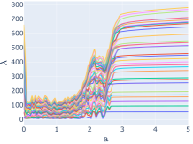
$\varepsilon=1,\mathbb{K}^{-1}|_{\Omega_{D}}=10^{3}$

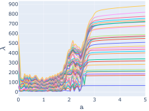
$\varepsilon=1,\mathbb{K}^{-1}|_{\Omega_{D}}=10^{5}$

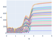
$\varepsilon=0,\mathbb{K}^{-1}|_{\Omega_{D}}=10^{-8}$

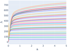
$\varepsilon=0,\mathbb{K}^{-1}|_{\Omega_{D}}=10^{3}$

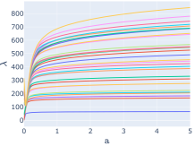
$\varepsilon=0,\mathbb{K}^{-1}|_{\Omega_{D}}=10^{5}$

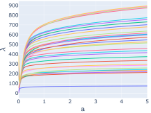
$\varepsilon=-1,\mathbb{K}^{-1}|_{\Omega_{D}}=10^{-8}$

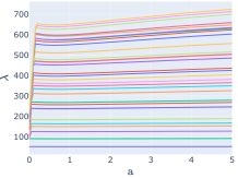
$\varepsilon=-1,\mathbb{K}^{-1}|_{\Omega_{D}}=10^{3}$

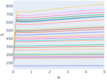
$\varepsilon=-1,\mathbb{K}^{-1}|_{\Omega_{D}}=10^{5}$

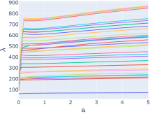
Figure 1: Test 6.1.1. Dependence of the spectrum on the stabilization parameter $\mathrm{a}>0$ in the three IPDG variants ($\varepsilon\in\{1,0,-1\}$), showing the first 40 lowest computed eigenvalues for different values of $\mathbb{K}$.

$\mathbb{K}^{-1}|_{\Omega_{D}}=10^{-8}\mathbb{I}$

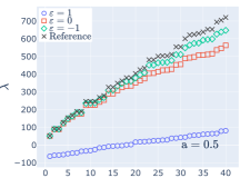
$\mathbb{K}^{-1}|_{\Omega_{D}}=10^{-8}\mathbb{I}$

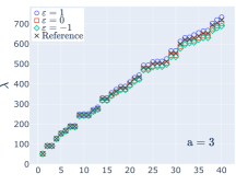
$\mathbb{K}^{-1}|_{\Omega_{D}}=10^{-8}\mathbb{I}$

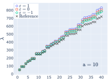
$\mathbb{K}^{-1}|_{\Omega_{D}}=10^{3}\mathbb{I}$

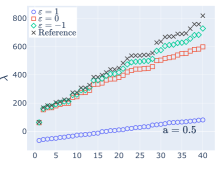
$\mathbb{K}^{-1}|_{\Omega_{D}}=10^{3}\mathbb{I}$

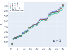
$\mathbb{K}^{-1}|_{\Omega_{D}}=10^{3}\mathbb{I}$

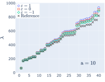
$\mathbb{K}^{-1}|_{\Omega_{D}}=10^{5}\mathbb{I}$

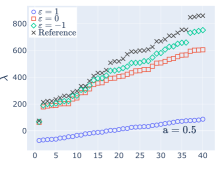
$\mathbb{K}^{-1}|_{\Omega_{D}}=10^{5}\mathbb{I}$

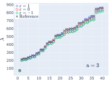
$\mathbb{K}^{-1}|_{\Omega_{D}}=10^{5}\mathbb{I}$

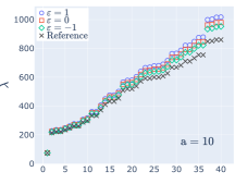
Figure 2: Test 6.1.1. Comparison of the first 40 lowest eigenvalues calculated with the three DG variants against the reference values from [25]

.

$\varepsilon=1,k=1$

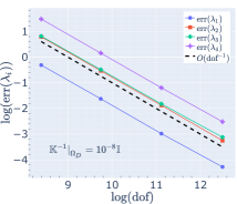
$\varepsilon=0,k=1$

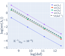
$\varepsilon=-1,k=1$

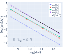
$\varepsilon=1,k=2$

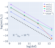
$\varepsilon=0,k=2$

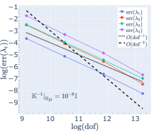
$\varepsilon=-1,k=2$

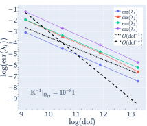
$\varepsilon=1,k=3$

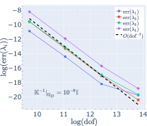
$\varepsilon=0,k=3$

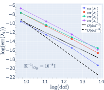
$\varepsilon=-1,k=3$

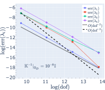
Figure 3: Test 6.1.2. Convergence history for the first four eigenvalues on each IPDG scheme for a selected stability parameter $\texttt{a}=10k^{2}$ and $\mathbb{K}^{-1}|_{\Omega_{D}}=10^{-8}$.

$\varepsilon=1,k=1$

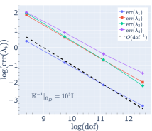
$\varepsilon=0,k=1$

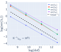
$\varepsilon=-1,k=1$

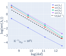
$\varepsilon=1,k=2$

$\varepsilon=0,k=2$

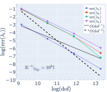
$\varepsilon=-1,k=2$

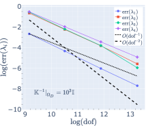
$\varepsilon=1,k=3$

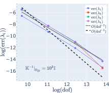
$\varepsilon=0,k=3$

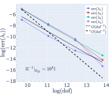
$\varepsilon=-1,k=3$

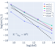
Figure 4: Test 6.1.2. Convergence history for the first four eigenvalues on each IPDG scheme for a selected stability parameter $\texttt{a}=10k^{2}$ and $\mathbb{K}^{-1}|_{\Omega_{D}}=10^{3}$.

6.2 Convergence on a 2D Lshaped porous domain with mixed boundary conditions

In this experment we put to the test the proposed scheme in the three variants of the method for a domain there there are singularities and mixed boundary conditions. The domain is the two-dimensional Lshape, defined as $\Omega:=(0,1)^{2}\backslash\left((0.5,0)\times(1,0.5)\right)$. We split the interior of $\Omega$ in such a way that there is an arrangement of different zones with given permeability parameters. A sample of the meshed geometry is depicted in Figure 5. Non-slip and do-nothing boundary conditions are assumed on $\Gamma_{1}$ and $\Gamma_{2}$, respectively. We take $\mathbb{K}$ such that $\mathbb{K}^{-1}=\boldsymbol{0}$ on $\Omega_{S}$, while $\mathbb{K}^{-1}=10^{3}\mathbb{I}$ on $\Omega_{D}$. On this test, the stabilization parameter is set to be $\texttt{a}=10$.

Taking as reference the suboptimal behavior observed in [25], we test the a posteriori estimator for $k=1$ in the three variants of the proposed DG scheme, while, due to the suboptimality predicted in Theorem 4.9 and therefore the lost efficiency of the estimator, we only consider the symmetric case for the higher order $k=2$.

In Figure 6 we present the adaptive meshes obtained by the DG variants for $k=1$. It is evident that our adaptive algorithm concentrates most of the refinements around the reentrant corner, as well as in regions with high pressure gradients. It is also worth noting that the number of elements marked inside the domain by the skew-symmetric method is higher than in the other schemes.

We conclude this test by presenting the error history and estimator efficiency for all IPDG schemes in Figures 8. In all cases, convergence rates of double order are observed, and the estimator remains both reliable and efficient, remaining bounded away from zero. For the symmetric case, a convergence rate of $\mathcal{O}(h^{2k})$ is clearly achieved. For the non-symmetric methods, the error curves and estimator efficiency exhibit very similar behavior and are optimal for $k=1$.

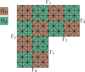
Figure 5: Test 6.2. Sample geometry of an Lshaped domain with a chessboard-like distribution of permeability regions and $N=10$.

$\lambda_{h,1},\varepsilon=1,\texttt{dof}=174678$

$\lambda_{h,1},\varepsilon=0,\texttt{dof}=204862$

$\lambda_{h,1},\varepsilon=-1,\texttt{dof}=229579$

$\lambda_{h,4},\varepsilon=1,\texttt{dof}=166467$

$\lambda_{h,4},\varepsilon=0,\texttt{dof}=167160$

$\lambda_{h,4},\varepsilon=-1,\texttt{dof}=178409$

Figure 6: Test 6.2. Last adaptive meshes for the first and fourth computed eigenvalue with for all the variants of the IPDG method in the Lshaped geometry with mixed boundary conditions and $\mathbb{K}^{-1}:=10^{3}\mathbb{I}$ on $\Omega_{D}$.

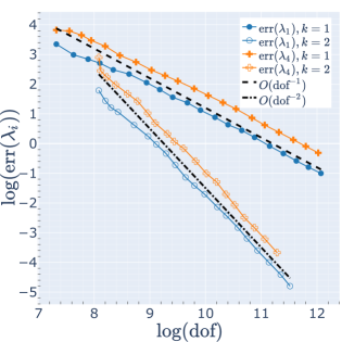
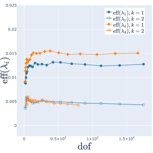
Figure 7: Test 6.2. Error history for the adaptive refinements when computing the first and fourth eigenvalue (left) together with their corresponding effectivity indexes (right) in the symmetric case ($\varepsilon=1$).

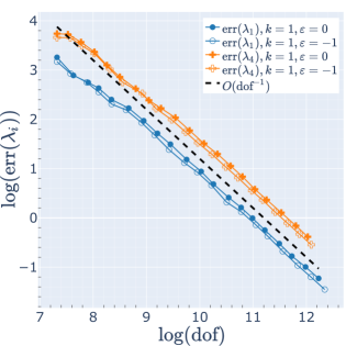
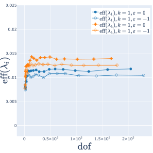
Figure 8: Test 6.2. Error history for the adaptive refinements when computing the first and fourth eigenvalue (left) together with their corresponding effectivity indexes (right) in the incomplete and skew-symmetric cases.

6.3 3D channel with a porous obstacle

We end the numerical section by presenting some results of the DG method on three-dimensional domains. For simplicity, we only consider the symmetric case $\varepsilon=1$. The domain under study is a box defined by $\Omega:=(0,1)\times(0,1)\times(0,3)$. Within this domain, we define the permeability parameter $\mathbb{K}$ as

$$\mathbb{K}^{-1}=\left\{\begin{aligned} &\kappa\mathbb{I}&\text{if }(x,y)\in\Omega_{D},\\ &\boldsymbol{0},&\text{if }(x,y)\in\Omega_{S},\end{aligned}\right.$$

where $\Omega_{D}:=(0,1)\times(1/3,2/3)\times(4/3,5/3)$ and $\Omega_{S}=\Omega\backslash\Omega_{D}$. We choose $\mathbb{K}^{-1}=10^{3}\mathbb{I}$. This choice allows to have a membrane-like behavior with partial permeability across $\Omega_{D}$. A graphical description of the domain is portrayed in Figure 9.

We solve the eigenvalue problem with $k=1,2$ and obtain the extrapolated discrete eigenvalue $\lambda_{1}=33.70064$, which is considered as the exact solution. Then, we perform 10 adaptive iterations for $k=1$ and 9 iterations for $k=2$ in order to observe the convergence rates and the reliability/efficiency of the estimator. The stabilization parameter is set to be $\texttt{a}=10$.

We present the corresponding lowest eigenmodes in Figure 10. Here, we observe the velocity field across the domain, entering and exiting through $\Gamma_{2}$, and we also note that some of the fluid, although with low magnitude, passes through the porous subdomain. This mild porosity causes high pressure gradients, represented by a concentrated cloud of points around $\Omega_{D}$. The eigenmode behavior is detected by the estimator and the adaptive algorithm, which marks the elements near the boundary of $\Omega_{D}$ for refinement. Some samples of the adaptive meshes for $k=1,2$ are presented in Figure 11, where critical singular zones are refined as expected. Similar to the 2D case, fewer elements are marked to achieve optimal rates for $k=2$.

The error and effectivity indices for the symmetric DG scheme are depicted in Figure 12. A rate $\mathcal{O}(\texttt{dof}^{-2k/d})$ is observed for $k\geq 1$ and $d=3$, implying an $h$-convergence rate of $\mathcal{O}(h^{2k})$. Moreover, the estimator effectivity remains properly bounded, demonstrating the reliability and efficiency of the estimator in the three-dimensional case with mixed boundary conditions.

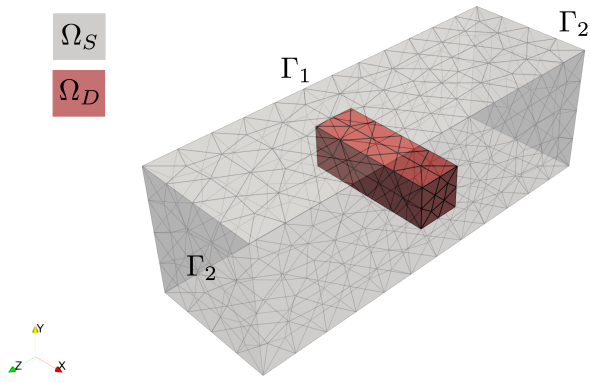
Figure 9: Test 6.3. The channel domain with the initial mesh configuration consisting of 2616 elements.

$\boldsymbol{u}_{h,1}$

$p_{h,1}$

Figure 10: Test 6.3. First lowest computed eigenmodes represented as the velocity field (top) and pressure dots cloud (bottom) in the last adaptive iteration.

$\texttt{dof}=76635$

$\texttt{dof}=324402$

$\texttt{dof}=1532895$

$\texttt{dof}=166600$

$\texttt{dof}=534344$

$\texttt{dof}=1200982$

Figure 11: Test 6.3. Intermediate adaptive meshes for $k=1,2,$ in the symmetric IPDG scheme ($\varepsilon=1$.)

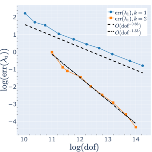
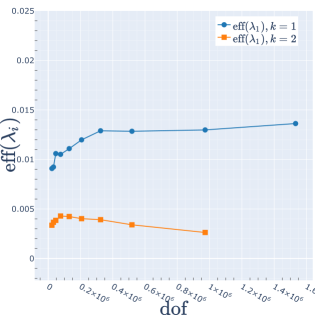
Figure 12: Test 6.3. Error history for the adaptive refinements when computing the first eigenvalue (left) together with their corresponding effectivity indexes (right) in the symmetric case ($\varepsilon=1$).

References

- [1] P. Acevedo Tapia, C. Amrouche, C. Conca, and A. Ghosh, Stokes and Navier-Stokes equations with Navier boundary conditions, J. Differential Equations, 285 (2021), pp. 258–320, https://doi.org/10.1016/j.jde.2021.02.045, https://doi.org/10.1016/j.jde.2021.02.045.
- [2] C. Amrouche and A. Rejaiba, -theory for Stokes and Navier-Stokes equations with Navier boundary condition, J. Differential Equations, 256 (2014), pp. 1515–1547, https://doi.org/10.1016/j.jde.2013.11.005, https://doi.org/10.1016/j.jde.2013.11.005.
- [3] P. F. Antonietti and B. Ayuso, Schwarz domain decomposition preconditioners for discontinuous Galerkin approximations of elliptic problems: non-overlapping case, M2AN Math. Model. Numer. Anal., 41 (2007), pp. 21–54, https://doi.org/10.1051/m2an:2007006.
- [4] P. F. Antonietti, A. Buffa, and I. Perugia, Discontinuous Galerkin approximation of the Laplace eigenproblem, Comput. Methods Appl. Mech. Engrg., 195 (2006), pp. 3483–3503, https://doi.org/10.1016/j.cma.2005.06.023.
- [5] P. F. Antonietti, S. Giani, and P. Houston, Domain decomposition preconditioners for discontinuous Galerkin methods for elliptic problems on complicated domains, J. Sci. Comput., 60 (2014), pp. 203–227, https://doi.org/10.1007/s10915-013-9792-y.
- [6] I. A. Barrata, J. P. Dean, J. S. Dokken, M. Habera, J. Hale, C. Richardson, M. E. Rognes, M. W. Scroggs, N. Sime, and G. N. Wells, DOLFINx: The next generation fenics problem solving environment, (2023), https://doi.org/10.5281/zenodo.10447666.
- [7] D. Boffi, Finite element approximation of eigenvalue problems, Acta Numer., 19 (2010), pp. 1–120, https://doi.org/10.1017/S0962492910000012.
- [8] S. C. Brenner, J. Cui, and L.-Y. Sung, Multigrid methods for the symmetric interior penalty method on graded meshes, Numer. Linear Algebra Appl., 16 (2009), pp. 481–501, https://doi.org/10.1002/nla.630.
- [9] A. Buffa, P. Houston, and I. Perugia, Discontinuous Galerkin computation of the Maxwell eigenvalues on simplicial meshes, J. Comput. Appl. Math., 204 (2007), pp. 317–333, https://doi.org/10.1016/j.cam.2006.01.042.
- [10] J. Descloux, N. Nassif, and J. Rappaz, On spectral approximation. I. The problem of convergence, RAIRO Anal. Numér., 12 (1978), pp. 97–112, iii, https://doi.org/10.1051/m2an/1978120200971.
- [11] J. Descloux, N. Nassif, and J. Rappaz, On spectral approximation. II. Error estimates for the Galerkin method, RAIRO Anal. Numér., 12 (1978), pp. 113–119, iii, https://doi.org/10.1051/m2an/1978120201131.
- [12] D. A. Di Pietro and A. Ern, Mathematical aspects of discontinuous Galerkin methods, vol. 69 of Mathématiques & Applications (Berlin) [Mathematics & Applications], Springer, Heidelberg, 2012, https://doi.org/10.1007/978-3-642-22980-0.
- [13] W. Dörfler, A convergent adaptive algorithm for poisson’s equation, SIAM Journal on Numerical Analysis, 33 (1996), pp. 1106–1124.
- [14] E. B. Fabes, C. E. Kenig, and G. C. Verchota, The Dirichlet problem for the Stokes system on Lipschitz domains, Duke Math. J., 57 (1988), pp. 769–793, https://doi.org/10.1215/S0012-7094-88-05734-1.
- [15] J. Gedicke and A. Khan, Divergence-conforming discontinuous galerkin finite elements for stokes eigenvalue problems, Numerische Mathematik, 144 (2020), pp. 585–614.
- [16] C. Geuzaine and J.-F. Remacle, Gmsh: A 3-D finite element mesh generator with built-in pre-and post-processing facilities, International journal for numerical methods in engineering, 79 (2009), pp. 1309–1331.
- [17] V. Girault, B. Rivière, and M. F. Wheeler, A discontinuous Galerkin method with nonoverlapping domain decomposition for the Stokes and Navier-Stokes problems, Math. Comp., 74 (2005), pp. 53–84, https://doi.org/10.1090/S0025-5718-04-01652-7, https://doi.org/10.1090/S0025-5718-04-01652-7.
- [18] P. Hansbo and M. G. Larson, Discontinuous Galerkin methods for incompressible and nearly incompressible elasticity by Nitsche’s method, Comput. Methods Appl. Mech. Engrg., 191 (2002), pp. 1895–1908, https://doi.org/10.1016/S0045-7825(01)00358-9.
- [19] V. Hernandez, J. E. Roman, and V. Vidal, SLEPc: A scalable and flexible toolkit for the solution of eigenvalue problems, ACM Transactions on Mathematical Software (TOMS), 31 (2005), pp. 351–362.
- [20] F. Lepe, Interior penalty discontinuous Galerkin methods for the velocity-pressure formulation of the Stokes spectral problem, Adv. Comput. Math., 49 (2023), pp. Paper No. 61, 31, https://doi.org/10.1007/s10444-023-10062-y.
- [21] F. Lepe, S. Meddahi, D. Mora, and R. Rodríguez, Mixed discontinuous Galerkin approximation of the elasticity eigenproblem, Numer. Math., 142 (2019), pp. 749–786, https://doi.org/10.1007/s00211-019-01035-9.
- [22] F. Lepe and D. Mora, Symmetric and nonsymmetric discontinuous Galerkin methods for a pseudostress formulation of the Stokes spectral problem, SIAM J. Sci. Comput., 42 (2020), pp. A698–A722, https://doi.org/10.1137/19M1259535.
- [23] F. Lepe, D. Mora, and J. Vellojin, Discontinuous Galerkin methods for the acoustic vibration problem, J. Comput. Appl. Math., 441 (2024), pp. Paper No. 115700, 21, https://doi.org/10.1016/j.cam.2023.115700.
- [24] F. Lepe, G. Rivera, and J. Vellojin, Finite element analysis of the oseen eigenvalue problem, Computer Methods in Applied Mechanics and Engineering, 425 (2024), p. 116959.
- [25] F. Lepe, G. Rivera, and J. Vellojin, A Stokes-Brinkman-type formulation for the eigenvalue problem in porous media, 2025, https://arxiv.org/abs/2507.08226, https://arxiv.org/abs/2507.08226.
- [26] S. Meddahi, A DG method for a stress formulation of the elasticity eigenproblem with strongly imposed symmetry, Comput. Math. Appl., 135 (2023), pp. 19–30, https://doi.org/10.1016/j.camwa.2023.01.022.
- [27] H. Paul, D. Schötzau, and T. P. Wihler, Energy norm shape a posteriori error estimation for mixed discontinuous Galerkin approximations of the Stokes problem, Journal of Scientific Computing, 22-23 (2005), p. 347 – 370, https://doi.org/10.1007/s10915-004-4143-7.
- [28] G. Savaré, Regularity results for elliptic equations in Lipschitz domains, J. Funct. Anal., 152 (1998), pp. 176–201, https://doi.org/10.1006/jfan.1997.3158.
- [29] L. R. Scott and S. Zhang, Finite element interpolation of nonsmooth functions satisfying boundary conditions, Math. Comp., 54 (1990), pp. 483–493, https://doi.org/10.2307/2008497.
- [30] M. W. Scroggs, I. A. Baratta, C. N. Richardson, and G. N. Wells, Basix: a runtime finite element basis evaluation library, Journal of Open Source Software, 7 (2022), p. 3982.
- [31] R. Verführt, A review of a posteriori error estimation and adaptive mesh-refinement techniques, Advances in numerical mathematics, Wiley, 1996.
- [32] K. Williamson, P. Burda, and B. Sousedík, A posteriori error estimates and adaptive mesh refinement for the Stokes–Brinkman problem, Mathematics and Computers in Simulation, 166 (2019), pp. 266–282.