Nesting-driven ferromagnetism of itinerant electrons

Abstract

We theoretically investigate a model with electrons and holes whose Fermi surfaces are perfectly nested. The fermions are assumed to be interacting, both with each other and with the lattice. To suppress inhomogeneous states, a sufficiently strong long-range Coulomb repulsion is included into the model. Using the mean field approximation, one can demonstrate that in the absence of doping, the ground state of such a model is insulating and possesses a density-wave order, either SDW, or CDW. Upon doping, a finite ferromagnetic polarization emerges. It is argued that the mechanism driving the ferromagnetism is not of the Stoner type. A phase diagram of the model is constructed, and various properties of the ordered phases are studied.

I Introduction

Can a gas of itinerant fermions with spin-independent repulsion exhibit the ferromagnetic state? This is one of the oldest research topics Bloch (1929) in theoretical condensed matter physics. Typically, the emergence of a finite ferromagnetic polarization of a Fermi gas is viewed through the lens of the so-called Stoner criterion. Since the moment of its inception almost one hundred years ago Stoner (1938), this theoretical device has become a standard tool employed in numerous original papers, and taught in various many-body-theory textbooks, both classical Huang (1987), and modern Blundell (2001).

The most seductive features of the Stoner criterion are its simplicity and universality: in the words of Kerson Huang (see p. 274 in Ref. Huang, 1987), “… if the repulsive strength is sufficiently strong, the system becomes ferromagnetic.” For numerous theoretical many-fermion models such a requirement is easy to benchmark against, and is not too restrictive, turning the criterion into an accessible tool to study a ferromagnetic instability. One can cite Refs. Zhou et al., 2021; Raines et al., 2024; Mohanta and Mishra, 2017 as recent examples of this approach.

Yet we must weight the simplicity of the Stoner framework against its unclear reliability. As the Stoner approach is an uncontrollable approximation, its accuracy can be assessed using numerical data only, which often conflict with the Stoner-criterion predictions (see, for instance, Ref. Holzmann and Moroni, 2020 and the discussion therein).

We believe that stable ferromagnetism in a system of itinerant fermions remains an important research issue of modern theoretical many-body physics. In this paper, we investigate a specific model where a ferromagnetic state can arise.

Unlike the Stoner approach, which becomes operational at moderate-to-strong inter-fermion repulsion, our model is in the weak-coupling regime, which is a significant advantage. Obviously, this implies that, at least in principle, the accuracy of the derived results can be tested using a suitably designed perturbative scheme, with the repulsion strength being a small parameter.

At the same time, in contrast to the all-encompassing universality of the Stoner criterion, our model relies on specific ingredients to generate stable ferromagnetism. Namely, we assume that the system is composed of both electrons and holes whose Fermi surfaces are nested. The fermions interact with each other via the Coulomb repulsion. In addition, the Hamiltonian of the model includes coupling between the fermions and lattice distortions at the nesting vector (this coupling is to some extent optional, since the ferromagnetic polarization can emerge without it). The main result of this study is the demonstration of a stable ferromagnetism in this model under doping. We also show that the ferromagnetic state is half-metallic, and, depending on model’s parameters, it possesses either perfect spin polarization of the Fermi surface states, or the so-called spin-flavor polarization Rozhkov et al. (2017); Rakhmanov et al. (2018).

The paper is organized as follows. The model itself is formulated in Sec. II. The ferromagnetism in the spin-density wave phase at nonzero is discussed in Sec. III. In Sec. IV, ferromagnetism of doped charge-density wave phase is studied. Section V presents the resultant phase diagram. Section VI is dedicated to the discussion.

II The model

The electron system with an interparticle repulsion and particle-lattice interaction is represented by the following Hamiltonian

$$H=H_{0}+H_{l}+H_{le}+H_{ee},$$ (1)

where $H_{0}$ is the Hamiltonian describing free electrons and holes, $H_{l}$ is the lattice deformation energy, $H_{le}$ is the term describing the interaction of electrons with the lattice and $H_{ee}$ is the electron-electron interaction.

To correctly construct the Hamiltonian of free electrons $H_{0}$, we divide the momentum space into separate sectors related to electrons and holes. The corresponding field operator $\psi$ is split into a sum of contributions with energies close to the Fermi energy

$$\psi_{\sigma}(\mathbf{r})=\psi_{\sigma,a}(\mathbf{r})+e^{i\mathbf{Q}\mathbf{r}}\psi_{\sigma,b}(\mathbf{r}),$$ (2)

where ${\bf Q}$ is the nesting vector, and partial field operators $\psi_{\sigma,a}$ and $\psi_{\sigma,b}$ are smooth on the scale $2\pi/|{\bf Q}|$. Decomposition (2) engenders related decomposition of the single-fermion Hamiltonian

$$H_{0}=\!\sum\limits_{\sigma}\!\int\!\!dV\!\Big{[}\psi_{\sigma,a}^{\dagger}\varepsilon_{a}(\mathbf{p})\psi_{\sigma,a}+\psi_{\sigma,b}^{\dagger}\varepsilon_{b}(\mathbf{p}+\mathbf{Q})\psi_{\sigma,b}\Big{]}.$$ (3)

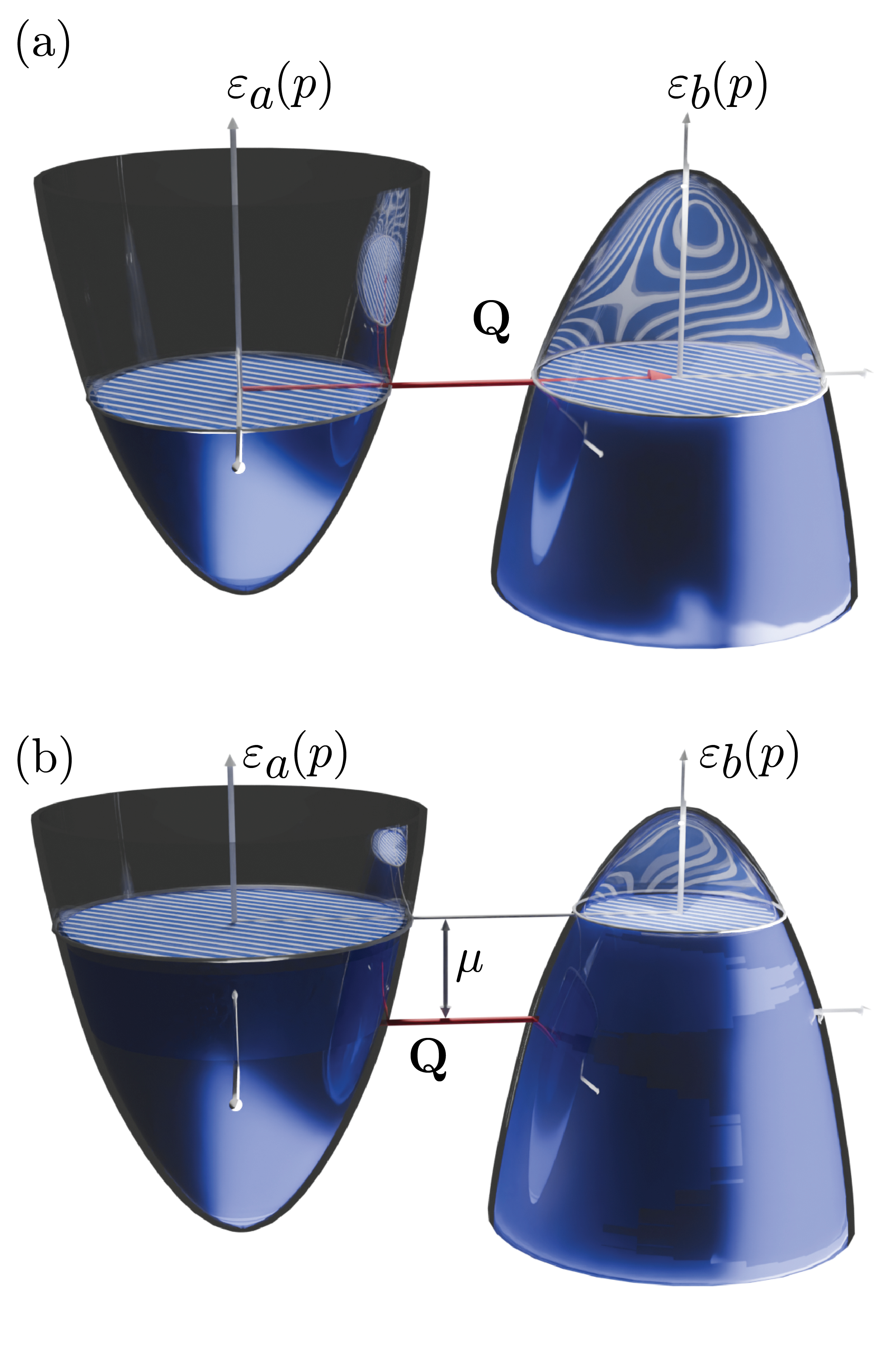
Figure 1: Single-fermion dispersion schematics. (a) The congruence of electron and hole cross sections of $\varepsilon_{a,b}$ - curves clearly demonstrate the nested Fermi surfaces separated by the nesting vector $\mathbf{Q}$. (b) The finite doping ($\mu$) destroys the ideal nesting of Fermi surfaces (unequal cross-sections).

In this formula, operators $\varepsilon_{a,b}$ are defined as follows

$$\begin{split}\varepsilon_{a}(\mathbf{p})&=\frac{\mathbf{p}^{2}-p_{\rm F}^{2}}{2m_{a}}-\mu,\\ \varepsilon_{b}(\mathbf{p}+\mathbf{Q})&=-\frac{\mathbf{p}^{2}-p_{\rm F}^{2}}{2m_{b}}-\mu,\end{split}$$ (4)

where $\mathbf{p}=-i\nabla$ (we use the units corresponding to $\hbar=0$). The first term in Eq. (3) corresponds to electron states, while the second term describes hole states (see Fig. 1). We assume that electrons and holes masses, $m_{a}$ and $m_{b}$, may be unequal $m_{a}\neq m_{b}$. To distinguish between electrons and holes in formulas, it is often convenient to introduce the so-called fermion-flavor quantum number $v_{\alpha}$, where $\alpha=a,b$, and $v_{a}=1$, $v_{b}=-1$.

If no doping is introduced into the system, the Fermi momenta of both electrons and holes are identical and equal to $p_{\rm F}$. Clearly, this is the case of perfect Fermi surface nesting: momentum-space translation on $\mathbf{Q}$ perfectly superimposes the electron Fermi surface sheet on the hole sheet. To describe a doped state, we introduce chemical potential $\mu$ in Eq. (4). Zero value of $\mu$ corresponds to the undoped state.

The particles interact with each other via the Coulomb repulsion

$$H^{C}_{ee}=\frac{1}{2}\int d\mathbf{r}\int d\mathbf{r}^{\prime}\frac{e^{2}}{\epsilon|\mathbf{r}-\mathbf{r}^{\prime}|}\rho(\mathbf{r})\rho(\mathbf{r}^{\prime}),$$ (5)

where $e$ is the elementary charge, and $\epsilon$ is the dielectric constant of the media. In connection with the density operator $\rho=\sum_{\sigma}\psi^{\dagger}_{\sigma}\psi^{\vphantom{{\dagger}}}_{\sigma}$, the following note is in order: due to the field operator decomposition (2), the particle density can be written as a sum of four terms

$$\rho(\mathbf{r})=\rho_{a}(\mathbf{r})+\rho_{b}(\mathbf{r})+e^{i\mathbf{Q}\mathbf{r}}\rho_{\mathbf{Q}}(\mathbf{r})+e^{-i\mathbf{Q}\mathbf{r}}\rho_{\mathbf{Q}}^{\dagger}(\mathbf{r}).$$ (6)

These partial densities are defined as

$$\rho_{a}=\sum_{\sigma}\psi^{\dagger}_{a,\sigma}\psi^{\vphantom{{\dagger}}}_{a,\sigma},\quad\rho_{b}=\sum_{\sigma}\psi^{\dagger}_{b,\sigma}\psi^{\vphantom{{\dagger}}}_{b,\sigma},$$ (7)

$$\rho_{\mathbf{Q}}^{\vphantom{{\dagger}}}=\sum_{\sigma}\psi^{\dagger}_{a,\sigma}\psi^{\vphantom{{\dagger}}}_{b,\sigma},\quad\rho_{\mathbf{Q}}^{\dagger}=\sum_{\sigma}\psi^{\dagger}_{b,\sigma}\psi^{\vphantom{{\dagger}}}_{a,\sigma}.$$ (8)

On the spatial scale $2\pi/|\mathbf{Q}|$, their variations are assumed to be insignificant.

As for $H^{C}_{ee}$ itself, we must remember that at low energies this “bare” interaction is renormalized by myriads of screening events. Thus, for a low-energy model, it is reasonaable to replace $H^{C}_{ee}$ with an effective interaction. It can be cast as a sum of direct and exchange point-like interactions

$$H_{ee}=H_{\rm dir}+H_{\rm ex},$$ (9)

$$H_{\rm dir}=g\sum\limits_{\sigma\sigma^{\prime}}\int dV\psi^{\dagger}_{\sigma,a}\psi_{\sigma,a}^{\vphantom{{\dagger}}}\psi^{\dagger}_{\sigma^{\prime},b}\psi_{\sigma^{\prime},b}^{\vphantom{{\dagger}}}+\ldots,$$ (10)

$$H_{\rm ex}=g_{\bot}\sum\limits_{\sigma\sigma^{\prime}}\int dV\psi^{\dagger}_{\sigma,a}\psi_{\sigma,b}^{\vphantom{{\dagger}}}\psi^{\dagger}_{\sigma^{\prime},b}\psi_{\sigma^{\prime},a}^{\vphantom{{\dagger}}}.$$ (11)

Here, the direct term $H_{\rm dir}$ represents couplings of the form $\rho_{a}\rho_{a}$, $\rho_{a}\rho_{b}$, and $\rho_{b}\rho_{b}$. They describe two-fermion collisions with a small momentum transfer. Since $\rho_{a}\rho_{b}$ plays a key role in the formation of ordered phases, it is explicitly shown in Eq. (10). The two other coupling types, $\rho_{a}\rho_{a}$ and $\rho_{b}\rho_{b}$, do not directly affect the ordering. Thus, we chose to replace them by ellipsis in Eq. (10).

The exchange term $H_{\rm ex}$ represents $\rho_{\mathbf{Q}}^{\vphantom{{\dagger}}}\rho_{\mathbf{Q}}^{\dagger}$ coupling. It describes collisions between an electron and a hole in which the electron (hole) is scattered to the hole (electron) Fermi surface sheet. Obviously, such a scattering event transfers large momentum $\sim\mathbf{Q}$. We expect that in a typical situation the effective coupling constants decrease when the transferred momentum grows. Thus, we have

$$g>g_{\bot}>0.$$ (12)

Both constants are positive due to the inter-particle interaction being repulsive.

Next, we introduce the Hamiltonian terms responsible for the electron-lattice coupling. For our analysis, it is sufficient to take the deformation energy of the lattice in its simplest form, discarding the shear modulus. Therefore, the Hamiltonian of the distorted lattice reads

$$H_{l}=\int\frac{K}{2}\varphi^{2}dV,$$ (13)

where $\varphi=\nabla\cdot\mathbf{u}$ and $\mathbf{u}$ is the strain vector, and $K$ is the bulk modulus. The quantum mechanical operator $\varphi$ is constructed based on its classical counterpart via a standard canonical quantization procedure [Abrikosov et al., 1975].

Likewise, the electrons’ interaction with the lattice is taken in the standard form [Abrikosov et al., 1975] of the electron-phonon interaction:

$$H_{le}=\eta\int\rho\varphi dV=\eta\sum\limits_{\sigma}\int\psi_{\sigma}^{\dagger}\psi_{\sigma}\varphi dV,$$ (14)

where $\eta$ is the electron-lattice coupling constant.

It is well-known that a Fermi surface with nesting is unstable with respect to formation of spin-density wave (SDW), or charge-density wave (CDW) ordered phases. To account for possible coupling between the CDW order parameter and electrons, we will be interested in a particular static distortion of the lattice with the wave vector $\mathbf{Q}$. Therefore, instead of considering the full dynamics of the lattice, we substitute the quantum mechanical operator $\varphi(\mathbf{r})$ with the classical potential profile

$$\varphi(\mathbf{r})=e^{i\mathbf{Q}\mathbf{r}}\varphi_{\mathbf{Q}}+e^{-i\mathbf{Q}\mathbf{r}}\varphi^{*}_{\mathbf{Q}},$$ (15)

where $\varphi_{\mathbf{Q}}$ and $\varphi_{\mathbf{Q}}^{*}$ represent classical lattice distortion mode with the wave vector $\mathbf{Q}$. Note that, due to the lattice dynamics being much slower than that of electrons, treating lattice degrees of freedom as classical static variables is admissible.

Combining the latter expression with Eqs. (6) and (14), we obtain the following Hamiltonian for lattice and electron-lattice interaction

$$H_{l}\!+\!H_{le}=K|\varphi_{\mathbf{Q}}|^{2}V\!+\!\eta\!\left(\!\varphi^{*}_{\mathbf{Q}}\sum\limits_{\sigma}\!\!\int\!\psi^{\dagger}_{\sigma,a}\psi_{\sigma,b}dV\!+\!{\rm H.c.}\!\right)\!\!,$$ (16)

where $V$ stands for the system volume.

III Spin density wave

As we already mentioned above, the instability of the nested Fermi surface in our model leads to the ordering with a density-wave-type order parameter. Depending on details, the order parameter is either SDW or CDW. The ferromagnetism we aim to describe in this paper can be viewed as a reaction of the density wave to doping affecting the gapped ordered environment. To substantiate this picture, we will use the mean field approximation to study the two types of density-wave order parameters, both with and without doping. In this section, we investigate the SDW, starting with the undoped case.

III.1 Undoped SDW state

To describe the SDW, we assume that the system acquires the nonzero field expectation value

$$\Delta_{\sigma}=g\langle\psi^{\dagger}_{a,\sigma}\psi_{b,\bar{\sigma}}^{\vphantom{{\dagger}}}\rangle.$$ (17)

Symbol $\bar{\sigma}$ in this formula represents the value opposite to $\sigma$. An SDW phase represented by this order parameter is polarized in $Oxy$ plane. The corresponding spin polarization in the coordinate space is

$$\left(\begin{matrix}S_{x}({\bf r})\\ S_{y}({\bf r})\\ \end{matrix}\right)=\frac{e^{i{\bf Q}\cdot{\bf r}}}{2g}\left(\begin{matrix}\Delta_{\uparrow}+\Delta_{\downarrow}\\ i\Delta_{\uparrow}-i\Delta_{\downarrow}\\ \end{matrix}\right)+{\rm C.c.}$$ (18)

Depending on relation between complex order parameters $\Delta_{\uparrow}$ and $\Delta_{\downarrow}$, the SDW can be either collinear or coplanar.

The mean field Hamiltonian corresponding to this order parameter reads

$$H_{\rm sdw}=\int\!\!dV\,\sum_{\sigma}\chi^{\dagger}_{\sigma}\mathcal{H}^{\rm sdw}_{\sigma}\chi^{\vphantom{{\dagger}}}_{\sigma}+\frac{V}{g}\sum_{\sigma}|\Delta_{\sigma}|^{2}.$$ (19)

where the spinor field $\chi_{\sigma}$ and a $2\times 2$ matrix ${\cal H}_{\sigma}^{\rm sdw}$ are defined according to

$${\cal H}_{\sigma}^{\rm sdw}=\begin{pmatrix}\varepsilon_{a}&-\Delta_{\sigma}\\ -\Delta^{*}_{\sigma}&\varepsilon_{b}\end{pmatrix},\quad\chi_{\sigma}=\begin{pmatrix}\psi_{a,\sigma}\\ \psi_{b,\bar{\sigma}}\end{pmatrix}.$$ (20)

Note that, within the mean field approximation, the fermionic fields in the SDW phase are evidently divided into two fermion sectors: sector $\sigma$ (sector $\bar{\sigma}$) contains $\psi_{a,\sigma}$ and $\psi_{b,\bar{\sigma}}$ fields ($\psi_{a,\bar{\sigma}}$ and $\psi_{b,{\sigma}}$ fields). Below we will see that this splitting occurs not only in the Hamiltonian, but in the self-consistency equations as well, and persists at finite doping. The concept of fermion sectors goes beyond simple notation convenience as the sectors will play pivotal role in our discussion of the doped system.

Another important observation is that neither $\varphi_{\mathbf{Q}}$ nor $g_{\bot}$ enter $H_{\rm sdw}$. Indeed, the CDW order parameter vanishes in the SDW phase. Thus, at the mean field level, the value of $\varphi_{\mathbf{Q}}$ is also zero, since $\varphi_{\mathbf{Q}}$ can couple to the CDW order parameter only, see Eq. (14). Likewise, $H_{\rm ex}$ describes interaction between two charge-density waves, and does not contribute to the spin-density channel.

Diagonalizing ${\cal H}_{\rm sdw}$, we obtain the following spectrum

$$\begin{split}E_{\sigma,\pm}({\bf p})&=\frac{\varepsilon_{a}({\bf p})+\varepsilon_{b}({\bf p})}{2}\pm\sqrt{\Big{[}\frac{\varepsilon_{a}({\bf p})-\varepsilon_{b}({\bf p})}{2}\Big{]}^{2}+|\Delta^{2}_{\sigma}|}.\end{split}$$ (21)

At zero temperature $T=0$, all states with $E_{\sigma,\pm}>0$ are empty, only the states with $E_{\sigma,\pm}<0$ contribute to the total energy $E$. It is equal to

$$E=\sum\limits_{\sigma,\mathbf{p}}E_{\sigma,-}(\mathbf{p})+\frac{V}{g}\sum_{\sigma}|\Delta_{\sigma}^{2}|.$$ (22)

Differentiating $E$ with respect to $\Delta_{\sigma}$, one can derive the following self-consistency equation

$$\Delta_{\sigma}=gN_{\rm F}\Delta_{\sigma}\mathfrak{I}_{\Lambda}(|\Delta_{\sigma}|).$$ (23)

In this formula, $N_{\rm F}$ is the density of states at the Fermi level

$$N_{\rm F}=\frac{p_{\rm F}m_{a}m_{b}}{\pi^{2}(m_{a}+m_{b})}=\frac{p_{\rm F}m_{\Sigma}}{4\pi^{2}}\gamma^{2},$$ (24)

where we introduced the notation:

$$\begin{split}\gamma&=\sqrt{1-\frac{\delta m^{2}}{m^{2}_{\Sigma}}}=\frac{2\sqrt{m_{a}m_{b}}}{m_{\Sigma}},\\ m_{\Sigma}&=m_{a}+m_{b},\quad\delta m=m_{b}-m_{a}.\end{split}$$ (25)

As for $\mathfrak{I}_{\Lambda}({\cal E})$ in Eq. (23), this function, being defined as

$$\mathfrak{I}_{\Lambda}({\cal E})=\int\limits_{0}^{\Lambda}\frac{p^{2}dp}{4\pi^{2}N_{\rm F}}\frac{1}{\sqrt{\frac{1}{4}[\varepsilon_{a}({\bf p})-\varepsilon_{b}({\bf p})]^{2}+\mathcal{E}^{2}}},$$ (26)

demonstrates the familiar logarithmic divergence in the limit of small ${\cal E}$

$$\mathfrak{I}_{\Lambda}({\cal E})\approx\ln\left(\frac{\varepsilon_{*}}{\cal E}\right),$$ (27)

where $\Lambda$ is large-momentum cutoff, $\varepsilon_{*}\sim\Lambda p_{\rm F}/(m_{1}+m_{2})$ is the corresponding ultraviolet energy cutoff.

One can see that expression (23) is a set of two decoupled equations labeled by index $\sigma$. Thus, as we mentioned before, the self-consistency equations for the two fermionic sectors are decoupled from each other. This feature is unique to the SDW mean field formalism, and it drastically simplifies our calculations. This simplification becomes particularly obvious when doped systems are studied.

Solving Eq. (23), we discover that, within each sector, there is either the trivial solution $\Delta_{\sigma}=0$, or

$$\Delta_{\sigma}=\Delta_{0}e^{i\Phi_{\sigma}},$$ (28)

where the energy scale

$$\Delta_{0}=\varepsilon_{*}e^{-\frac{1}{gN_{\rm F}}},$$ (29)

satisfies a BCS-type equation

$$\frac{1}{gN_{\rm F}}=\mathfrak{I}_{\Lambda}(\Delta_{0}).$$ (30)

Phases $\Phi_{\sigma}$ remain undetermined by the self-consistency equations, and can be chosen arbitrary.

The many-electron state with $\Delta_{\sigma}=0$ is unstable, and the ground state is described by Eq. (28) for both $\sigma=\uparrow,\downarrow$. Since the order parameters are finite in both sectors, we conclude that the mean field SDW phase is insulating as its spectrum (21) has a gap

$$\Delta E=2\gamma\Delta_{0}.$$ (31)

This gap is not direct: the bottom of the conduction band is not at $p=p_{\rm F}$, but rather is at $p_{\rm c}=p_{\rm F}-\gamma\delta m\Delta_{0}/(4p_{\rm F})$, while the top of the valence band is at $p_{\rm v}=p_{\rm F}+\gamma\delta m\Delta_{0}/(4p_{\rm F})$, and $p_{\rm c}\neq p_{\rm v}$. In the limit of equal masses $m_{a}=m_{b}$, this gap becomes direct and equal to $2\Delta_{0}$.

Once we solve the self-consistency equations, we obtain the standard formula for the ground state energy

$$F_{0}=-N_{\rm F}\Delta_{0}^{2}V.$$ (32)

Next, using Eq. (18), we calculate SDW spin polarization in coordinate space

$$\left(\begin{matrix}S_{x}({\bf r})\\ S_{y}({\bf r})\\ \end{matrix}\right)=\frac{2\Delta_{0}}{g}\left(\begin{matrix}\cos\Phi\\ \sin\Phi\\ \end{matrix}\right)\cos({\bf Q}\cdot{\bf r}+\phi).$$ (33)

The value of $\phi=(\Phi_{\sigma}-\Phi_{\bar{\sigma}})/2$ determines overall space translation of the SDW texture, while $\Phi=(\Phi_{\sigma}+\Phi_{\bar{\sigma}})/2$ sets the direction along which the SDW is polarized. Spin polarization (33) is explicitly collinear.

The degeneracy with respect to $\Phi$ is a consequence of model’s spin-rotation symmetry. This degeneracy cannot be lifted unless the latter is broken. The degeneracy relative to $\phi$ may be removed, at least partially, if lattice effects are introduced in the form of umklapp terms. For example, if $2\mathbf{Q}$ is either zero or a reciprocal lattice vector, umklapp couplings with structure $\psi^{\dagger}_{a,\sigma}\psi^{\vphantom{{\dagger}}}_{b,\sigma}\psi^{\dagger}_{a,\sigma^{\prime}}\psi^{\vphantom{{\dagger}}}_{b,\sigma^{\prime}}$ and $\psi^{\dagger}_{b,\sigma}\psi^{\vphantom{{\dagger}}}_{a,\sigma}\psi^{\dagger}_{b,\sigma^{\prime}}\psi^{\vphantom{{\dagger}}}_{a,\sigma^{\prime}}$ become permissible. They “pin” the SDW to the lattice, which restricts possible values of $\phi$ to a finite set.

III.2 SDW at finite doping

Adding charge carriers, either electrons or holes, destroys perfect nesting of the Fermi surface in our system (see Fig. 1). The doped state has a tendency toward the formation of spatially inhomogeneous states, which have been studied in numerous publications in various contexts Gorbatsevich et al. (1992); Gor’kov and Teitel’baum (2010); Igoshev et al. (2010, 2015); Rakhmanov et al. (2017, 2020); Kokanova et al. (2021); M. Yu. Kagan et al. (2021, 2024). Sufficiently strong Coulomb long-range repulsion restores the stability of a homogeneous phase, causing system to lower its energy by implementing a kind of phase separation that occurs in space of discrete indices, instead of continuous coordinate space Rozhkov et al. (2017); Rakhmanov et al. (2018); Khokhlov et al. (2020); Sboychakov et al. (2020, 2021); Rakhmanov et al. (2023). In such a regime interaction effects force uneven distribution of electrons among available discrete quantum numbers. This unevenness, as we will demonstrate in this section, is ultimately responsible for stabilization of a ferromagnetic phase in our model.

On the technical side, to introduce doping into the formalism, we will assume that the chemical potential is no longer zero. For definiteness, $\mu>0$ case is studied below. Adaptation for negative $\mu$ is quite straightforward. We also assume the doping level to be rather small

$$\mu\ll\frac{p_{\rm F}^{2}}{m_{\Sigma}}$$ (34)

to be able to capture the richest physics attributed to the density wave gap formation.

Thus, the grand canonical potential $\Omega$ for finite $\mu$ is a sum $\Omega=\sum_{\sigma}\Omega_{\sigma}$, where a partial potential for sector $\sigma$ is

$$\Omega_{\sigma}=\frac{V}{g}|\Delta_{\sigma}|^{2}+\sum\limits_{\mathbf{p}}[E_{\sigma,-}(\mathbf{p})-\mu]+$$ (35)

$$\sum\limits_{\mathbf{p}}[E_{\sigma,+}(\mathbf{p})-\mu]\theta(\mu-E_{\sigma,+}(\mathbf{p})),$$

where $\theta(x)$ is the Heaviside step-function. Here, the first sum represents the energy of the filled hole band, while the second sum gives the energy of the pocket of the electron band (see Fig. 2). For an undoped system, Eq. (28) implies that both fermionic sectors have identical values of $|\Delta_{\sigma}|$. This equivalence may be broken as soon as doping is introduced: it is argued in Ref. Rakhmanov et al., 2018 that, not only $|\Delta_{\sigma}|$ may differ from $|\Delta_{\bar{\sigma}}|$, the doped electrons may be distributed between the sectors unevenly.

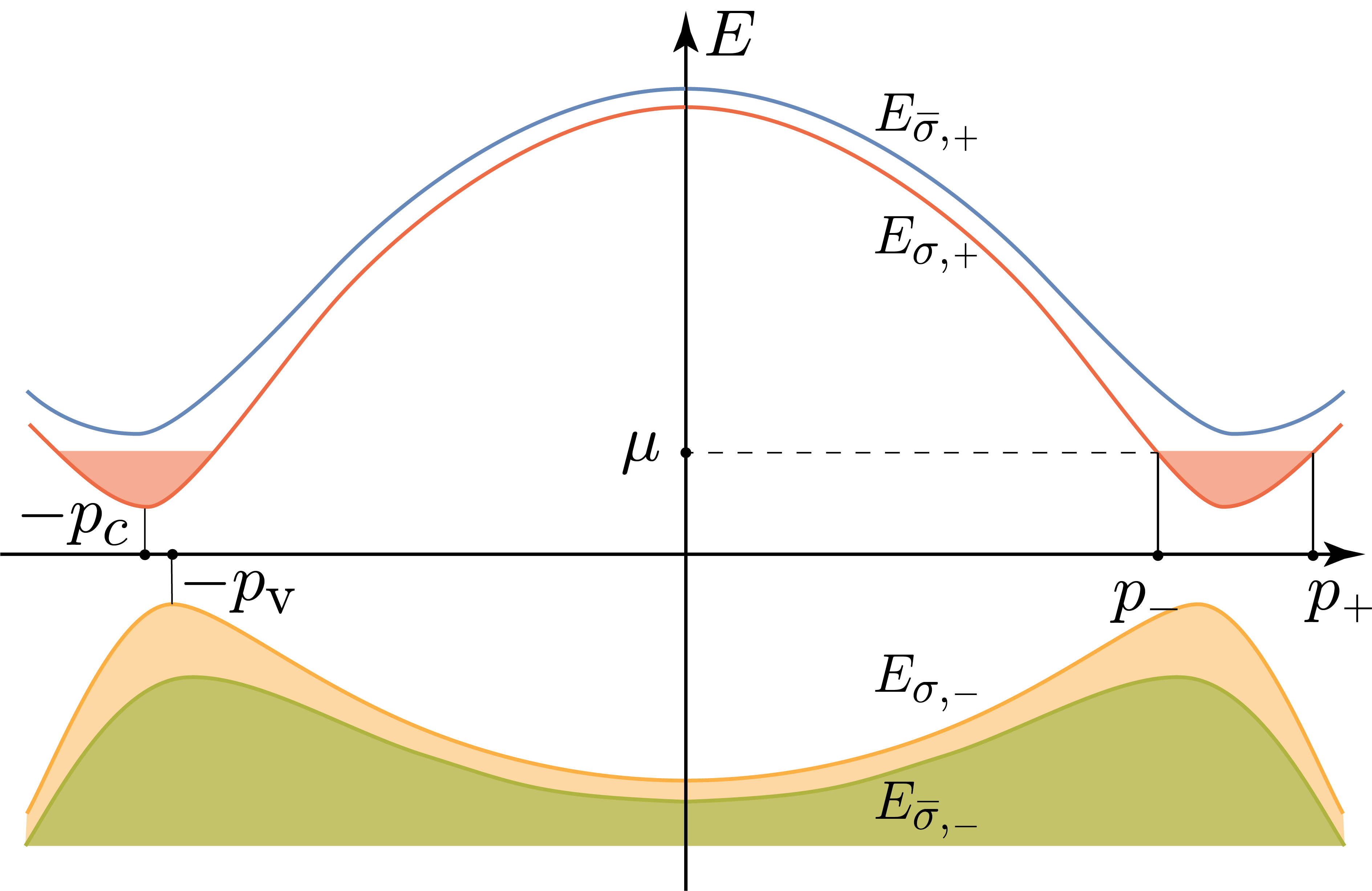
Figure 2: Dispersion curves $E_{\sigma,\pm}$, see Eq. (21), for doped state. The electron mass $m_{a}$ is larger than the hole mass $m_{b}$. To simplify the drawing, we assumed that the nesting vector ${\bf Q}$ is zero. Vertical axis represents energy, horizontal axis is momentum $p$. The chemical potential level is shown by the horizontal dashed line. Two sectors are doped differently: one is empty (the corresponding dispersion curve lies above $\mu$), the other one contains all extra charges accumulated between $p_{-}$ and $p_{+}$. The minimum of the conduc- tion band $p_{c}$, differs from the maximum of the valence band $p_{\rm v}$ marking the indirect gap (see the discussion after Eq. (31).)

To accommodate for this possibility, it is useful to introduce partial doping concentrations $x_{\sigma}=-\partial\Omega_{\sigma}/\partial\mu$, whose sum equals to total doping $x_{\sigma}+x_{\bar{\sigma}}=x$. One can easily establish that

$$x_{\sigma}=\int\limits_{0}^{+\infty}\frac{p^{2}dp}{2\pi^{2}}\theta(\mu-E_{\sigma,+})\approx\frac{p_{\rm F}(p_{+}^{2}-p_{-}^{2})}{4\pi^{2}},$$ (36)

where the momenta

$$p_{\pm}=\sqrt{p_{\rm F}^{2}-\delta m\mu\pm m_{\Sigma}\sqrt{\mu^{2}-\gamma^{2}|\Delta^{2}_{\sigma}|}}$$ (37)

define two Fermi surfaces in sector $\sigma$, see Fig. 2. Combining the latter two equations, we ultimately derive

$$x_{\sigma}=\frac{2N_{\rm F}}{\gamma^{2}}\sqrt{\mu^{2}-\gamma^{2}|\Delta_{\sigma}^{2}|}.$$ (38)

Clearly, the square root in this formula is real only when

$$\mu>\gamma|\Delta_{\sigma}|.$$ (39)

This is the condition for sector $\sigma$ being doped. If this inequality is violated, the sector is empty of extra charges. The situation, when one sector is doped, while the other is empty is schematically shown in Fig. 2. We will argue below that, at not too high doping, this corresponds to the ground state of our model.

For doping $x$ fixed externally, we need to find $\mu$, $\Delta_{\sigma}$, and $\Delta_{\bar{\sigma}}$. Thus, three equations must be determined and then solved. One such equation is a constraint

$$x=\frac{2N_{\rm F}}{\gamma^{2}}\sum_{\sigma}\sqrt{\mu^{2}-\gamma^{2}|\Delta_{\sigma}^{2}|},$$ (40)

which one obtains using Eq. (38). Two minimization conditions $\partial\Omega/\partial\Delta_{\sigma}=0$ complete the desired set of three equations. Performing the differentiation, one derives the self-consistency equations

$$\mathfrak{I}_{\mu}(\Delta_{\sigma})=\frac{1}{gN_{\rm F}},$$ (41)

where function $\mathfrak{I}_{\mu}$ is introduced according to

$$\mathfrak{I}_{\mu}(\Delta_{\sigma})=\mathfrak{I}_{\Lambda}(|\Delta_{\sigma}|)-\int\limits_{p_{-}}^{p_{+}}\frac{p^{2}dp}{4\pi^{2}N_{\rm F}}\frac{\theta(\mu-\gamma|\Delta_{\sigma}|)}{\sqrt{\Big{(}\frac{\varepsilon_{a}-\varepsilon_{b}}{2}\Big{)}^{2}+|\Delta_{\sigma}^{2}|}}.$$ (42)

Note that, in this definition, the integration limits $p_{\pm}=p_{\pm}(\Delta_{\sigma})$ are set by Eq. (37), while the integral itself represents the effect of charge carriers inserted into the system on the system properties. Ultimately, one evaluates

$$\mathfrak{I}_{\mu}(\Delta_{\sigma})\approx\ln\left(\frac{\varepsilon_{*}}{|\Delta_{\sigma}|}\right)-\ln\left(\frac{\mu+\sqrt{\mu^{2}-\gamma^{2}|\Delta_{\sigma}^{2}|}}{\gamma|\Delta_{\sigma}|}\right)$$ (43)

in the leading log approximation. Subtracting Eq. (30) from Eq. (41) and exploiting the smallness of $\mu$ (see Eq. 53), we obtain the following relation between $\mu$ and $|\Delta_{\sigma}|$

$$\ln\left(\frac{\mu+\sqrt{\mu^{2}-\gamma^{2}|\Delta_{\sigma}^{2}|}}{\gamma|\Delta_{\sigma}|}\right)-\ln\frac{\Delta_{0}}{|\Delta_{\sigma}|}=0.$$ (44)

Using Eq. (38) one can finally establish the relation between $x_{\sigma}$ and $\Delta_{\sigma}$

$$|\Delta_{\sigma}|=\Delta_{0}\sqrt{1-\frac{x_{\sigma}\gamma}{N_{\rm F}\Delta_{0}}}.$$ (45)

We see that, as anticipated, the SDW sectors remain decoupled even at finite doping. Also, $|\Delta_{\sigma}|$ is a decreasing function of the partial doping: for finite $x_{\sigma}$, one has $|\Delta_{\sigma}|<\Delta_{0}$.

It is not difficult to demonstrate that the chemical potential is a linear function of the partial doping

$$\mu=\Delta_{0}\gamma-\frac{\gamma^{2}x_{\sigma}}{2N_{\rm F}}.$$ (46)

In addition, one might conclude that this formula immediately implies that $x_{\sigma}=x_{\bar{\sigma}}$: the chemical potential is the same for both sectors, so must be partial doping concentrations.

However, the latter reasoning is, in fact, incorrect. Let us remind the reader that, per our assumption at the beginning of the derivation, both Eqs. (45) and (46) are valid for finite $x_{\sigma}$ only. When inequality (39) is satisfied for sector $\sigma$, but violated for sector $\bar{\sigma}$, then all the doping is in sector $\sigma$, while $x_{\bar{\sigma}}\equiv 0$.

This suggests that, at finite doping $x$, we have two possibilities:

$${\rm Sym.\ case:} x_{\sigma}=x_{\bar{\sigma}}=x/2,$$ (47)

$${\rm Asym.\ case:} x_{\sigma}=x,\quad x_{\bar{\sigma}}=0.$$ (48)

These states have non-identical free energies. Indeed, a partial (per sector) free energy $F_{\sigma}=F_{\sigma}(x_{\sigma})$ associated with doping reads

$$\frac{F_{\sigma}(x_{\sigma})}{V}=\int_{0}^{x_{\sigma}}\mu(x_{\sigma}^{\prime})dx_{\sigma}^{\prime}=\gamma\Delta_{0}x_{\sigma}-\frac{\gamma^{2}x_{\sigma}^{2}}{4N_{\rm F}}.$$ (49)

The total free energy $F=F_{0}+F_{\sigma}+F_{\bar{\sigma}}$, where $F_{0}$ is the free energy of the undoped state (see Eq. 32), can be expressed as

$$\frac{F}{V}=-N_{\rm F}\Delta_{0}^{2}+\gamma\Delta_{0}x-\frac{\gamma^{2}}{4N_{\rm F}}(x_{\sigma}^{2}+x_{\bar{\sigma}}^{2}).$$ (50)

We therefore have

$${\rm Sym.\ case:} \frac{F_{\rm S}}{V}=-N_{\rm F}\Delta_{0}^{2}+\gamma\Delta_{0}x-\frac{\gamma^{2}}{8N_{\rm F}}x^{2},$$ (51)

$${\rm Asym.\ case:} \frac{F_{\rm A}}{V}=-N_{\rm F}\Delta_{0}^{2}+\gamma\Delta_{0}x-\frac{\gamma^{2}}{4N_{\rm F}}x^{2}.$$ (52)

Comparing the two free energies, we conclude that asymmetric state, where all extra electrons are placed into a single sector, corresponds to the lowest energy. In other words, Fig. 2 depicts the state with the lowest energy.

III.3 Properties of the half-metal state

Characteristic feature of the doped SDW has been discussed in several publications Rozhkov et al. (2017); Rakhmanov et al. (2018); Sboychakov et al. (2020); Khokhlov et al. (2020); Sboychakov et al. (2021); Rakhmanov et al. (2023) in different contexts. Thus, we limit ourselves here to a brief discussion only. We start with the observation that Eqs. (51) and (52), taken at their face value, clearly reveal instability toward the phase separation. Indeed, using the relation $\mu=\partial F/\partial x$, one can derive

$${\rm Sym.\ case:} \mu_{\rm S}=\gamma\Delta_{0}-\frac{\gamma^{2}}{4N_{\rm F}}x,$$ (53)

$${\rm Asym.\ case:} \mu_{\rm A}=\gamma\Delta_{0}-\frac{\gamma^{2}}{2N_{\rm F}}x.$$ (54)

Both $\mu_{\rm S}$ and $\mu_{\rm A}$ are decreasing functions of doping, which is a signature of the instability towards formation of spatially inhomogeneous structures (in stable systems $\partial\mu/\partial x>0$).

As electrons are charged particles, the possibility for forming spatially varying distributions of electrons is severely constrained by the long-range Coulomb interaction (5). Below, we will always assume that the long-range forces are sufficiently strong to guarantee perfect homogeneity of our system.

Second, Eq. (45) indicates that the doping reduces the strength of the SDW order. For $x>N_{\rm F}\Delta_{0}/\gamma$ the order parameter in the charge-carrying sector is zero. At critical value $x=N_{\rm F}\Delta_{0}/\gamma$ one cannot accomodate all the particles in a single sector, and the symmetric state sets in.

Third, it is important to remember that the ground state is a kind of a metal: there are single-electron states reaching the chemical potential, as Fig. 2 illustrates. There are concentric Fermi surface sheets, whose radii are $p_{\pm}$.

However, this is not a usual metal, but rather is an example of half-metal: of four possible types of fermions (electrons/hole, with spin-up/down), only two of these four types (that is, a half) reach the Fermi level. Unlike “classical” half-metallic phase de Groot et al. (1983), which demonstrates perfect spin polarization of the Fermi surface, our asymmetric state is perfectly polarized in terms of the spin-flavor index.

To explain, what this index is, let us define the spin-flavor operator as

$$S_{\rm sf}=\sum_{\sigma,\alpha}\sigma v_{\alpha}\int dV\psi^{\dagger}_{\sigma,\alpha}\psi^{\vphantom{{\dagger}}}_{\sigma,\alpha},$$ (55)

where $v_{\alpha}$ is the fermion-flavor quantum number, see Sec. II. The presence of $v_{\alpha}$ in Eq. (55) distinguishes $S_{\rm sf}$ from the familiar $z$-axis spin-projection operator

$$S_{z}=\sum_{\sigma,\alpha}\sigma\int dV\psi^{\dagger}_{\sigma,\alpha}\psi^{\vphantom{{\dagger}}}_{\sigma,\alpha},$$ (56)

The field operators satisfy obvious commutation rules $[S_{\color[rgb]{0,0,1}z},\psi_{\sigma,\alpha}]=\sigma\psi_{\sigma,\alpha}$, and $[S_{\rm{\color[rgb]{0,0,1}sf}},\psi_{\sigma,\alpha}]=\sigma v_{\alpha}\psi_{\sigma,\alpha}$. Therefore, in addition to the spin quantum number $\sigma$, a field $\psi_{\sigma,\alpha}$ can be characterized by the spin-flavor projection $\sigma v_{\alpha}$.

It is easy to check that in the sector $\sigma$, both $\psi_{\sigma,a}$ and $\psi_{{\bar{\sigma}},b}$ carry the same spin-flavor quantum equal to $+\sigma$. In the sector ${\bar{\sigma}}$, the field operators correspond to a ${-\sigma}$ quantum of $S_{\rm sf}$. That is, the Fermi surface of the doped system is characterized by the single projection of the spin-flavor operator. The Fermi surface sheet with the opposite projection of $S_{\rm sf}$ is absent, since the sector ${\bar{\sigma}}$ is gapped. Thus, due to the Fermi surface polarization in terms of spin-flavor index, the doped system can be referred to as a spin-flavor half-metal (SFHM).

III.4 The ferromagnetic polarization of the half-metal phase

Simple calculations Rozhkov et al. (2017) allow one to prove that total spin-flavor polarization of the SFHM state is proportional to the doping $\langle S_{\rm sf}\rangle=\sigma xV$. It is perhaps less obvious, but more important from a fundamental perspective, that this state possesses finite spin polarization $\langle S_{z}\rangle\neq 0$. Within the mean field approximation,

$$\langle S_{z}\rangle\!=\!\!\int\limits_{p_{-}}^{p_{+}}\frac{p^{2}dp}{2\pi^{2}}s(|\Delta_{\sigma}|)-\!\!\int\limits_{0}^{\infty}\frac{p^{2}dp}{2\pi^{2}}s(|\Delta_{\sigma}|)+\!\!\int\limits_{0}^{\infty}\frac{p^{2}dp}{2\pi^{2}}s(\Delta_{0}),\quad$$ (57)

where function $s=s({\cal E})$ is defined as

$$s({\cal E})=\frac{\varepsilon_{a}-\varepsilon_{b}}{\sqrt{\Big{(}\varepsilon_{a}-\varepsilon_{b}\Big{)}^{2}+4{\cal E}^{2}}}.$$ (58)

The first term in the right-hand side of Eq. (57) represents the contribution of the doped conduction band in sector $\sigma$. The second and the third terms correspond to contributions of completely filled valence bands in sectors $\sigma$ and $\bar{\sigma}$. These two terms sum up into the expression that is small, of the order of $p_{\rm F}^{3}\big{[}\mathcal{O}(a^{2}\ln a)\big{]}$, where $a=|\Delta_{\sigma}|m_{\Sigma}/p_{\rm F}^{2}\ll 1$ is a small parameter. The contribution due to the doped conduction band, however, produces the answer of the order of $p_{\rm F}^{3}\mathcal{O}(a)$. It is easily computed, and we have the following expression for the spin polarization of SDW in the leading approximation

$$\langle S_{z}\rangle\approx-x\frac{\delta m}{m_{\Sigma}}.$$ (59)

We see that this expression is finite only when the symmetry between electrons and holes is broken $\delta m\neq 0$. Otherwise, $\langle S_{z}\rangle$ is zero.

Beside $\langle S_{z}\rangle$, the $Oxy$ polarization (18) remains nonzero. Using the latter formula, we derive

$$\left(\begin{matrix}S_{x}\\ S_{y}\\ \end{matrix}\right)=\frac{1}{g}\left(\begin{matrix}|\Delta_{\uparrow}|\cos(\mathbf{Qr}+\Phi_{\uparrow})+|\Delta_{\downarrow}|\cos(\mathbf{Qr}+\Phi_{\downarrow})\\ -|\Delta_{\uparrow}|\sin(\mathbf{Qr}+\Phi_{\uparrow})+|\Delta_{\downarrow}|\sin(\mathbf{Qr}+\Phi_{\downarrow})\\ \end{matrix}\right).$$ (60)

To make this formula more transparent, let us introduce a complex quantity ${\cal S}({\bf r})=S_{x}+iS_{y}$. It reads

$${\cal S}=(|\Delta_{\uparrow}|e^{-2i\mathbf{Q}{\bf r}-2i\Phi}+|\Delta_{\downarrow}|)e^{i\mathbf{Q}{\mathbf{r}}+i\Phi_{\downarrow}}.$$ (61)

Since the order parameters are not identical, ${\cal S}$ never vanishes. This implies that the $xy$ polarization is not collinear any more.

Assuming for definiteness that $|\Delta_{\uparrow}|<|\Delta_{\downarrow}|$, one can check trivially that, as $\mathbf{Q}\mathbf{r}$ changes from zero to $2\pi$, function ${\cal S}$ winds once around the complex plane origin. This means that local spin polarization vector

$${\bf S}({\bf r})=(S_{x}({\bf r}),S_{y}({\bf r}),S_{z})^{T}$$ (62)

sweeps out a cone as the observation point ${\bf r}$ moves along the nesting vector $\mathbf{Q}$ (see Fig. 3).

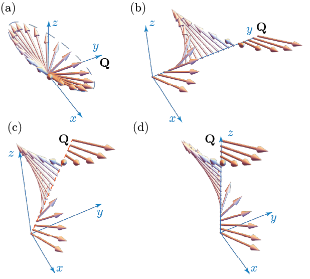
Figure 3: Magnetization vector behavior for different orientation of nesting vector $\mathbf{Q}$ as radius vector $\mathbf{r}$ moves along $\mathbf{Q}$. For illustrative purposes, we choose $|\Delta_{\downarrow}|/|\Delta_{\uparrow}|=2$ and $S_{z}=1.3|\Delta_{\uparrow}|/g$. (a) The magnetic polarization vectors (laid off from the same point) sweeping out a conical shape, as the radius vector $\mathbf{r}$ moves along the nesting vector $\mathbf{Q}$. (b-d): the behavior of magnetization vector in coordinate space. (b) $\mathbf{Q}$ is oriented in $y$ direction. (c) $\mathbf{Q}$ direction is shown with the dashed line, $\mathbf{Q}\propto[0,1/\sqrt{5},2/\sqrt{5}]$. (d) $\mathbf{Q}\propto[0,0,1]$, the helical structure is clearly pronounced.

IV Charge density wave

In this section, we investigate the doped CDW phase using the mean field approximation. Dissimilar to the SDW, both exchange and electron-lattice interactions explicitly enter the CDW calculations. While these contributions introduce additional complications to theoretical framework, many features are shared between the SDW and the CDW formalisms.

The CDW corresponds to a different order parameter

$$\Delta\equiv\sum\limits_{\sigma}\Delta_{\sigma},\quad\text{where}\quad\Delta_{\sigma}^{\vphantom{{\dagger}}}=g\langle\psi^{\dagger}_{\sigma,a}\psi_{\sigma,b}^{\vphantom{{\dagger}}}\rangle.$$ (63)

It represents spatially modulated density of charge carriers

$$\rho({\bf r})\!\propto\!(\Delta_{\sigma}\!+\!\Delta_{\bar{\sigma}})e^{-i{\bf Q}\cdot{\bf r}}\!+{\rm C.c.}=\!2|\Delta|\cos({\bf Q}\!\cdot\!{\bf r}).$$ (64)

Here, the origin is assumed to be chosen in a way to eliminate the additional constant phase in the argument of the cosine. This order parameter is affected by both interaction terms, $H_{\rm dir}$ and $H_{\rm ex}$: the former enhances the CDW, the latter suppresses it. Additionally, it couples to the lattice distortion $\varphi_{\mathbf{Q}}$, which acts as a stabilization factor for the CDW.

The mean field Hamiltonian for the CDW state can be expressed as

$$H_{\rm cdw}=\int\!\!dV\,\sum_{\sigma}\zeta^{\dagger}_{\sigma}{\cal H}_{\sigma}^{\rm cdw}\zeta^{\vphantom{{\dagger}}}_{\sigma}+V\mathfrak{E}_{0}^{\rm cdw},$$ (65)

where a $2\times 2$ matrix ${\cal H}_{\sigma}^{\rm cdw}$ and spinor field $\zeta_{\sigma}$ are equal to

$${\cal H}_{\sigma}^{\rm cdw}=\begin{pmatrix}\varepsilon_{a}&-D_{\sigma}\\ -D_{\sigma}^{*}&\varepsilon_{b}\end{pmatrix},\quad\zeta_{\sigma}=\begin{pmatrix}\psi_{a,\sigma}\\ \psi_{b,\sigma}\end{pmatrix},$$ (66)

where

$$D_{\sigma}=\Delta_{\sigma}-\frac{g_{\bot}}{g}\Delta-\eta\varphi_{\mathbf{Q}},$$ (67)

Finally, a $c$-number constant

$$\mathfrak{E}_{0}^{\rm cdw}=-\frac{g_{\bot}}{g^{2}}|\Delta|^{2}+\frac{1}{g}\sum\limits_{\sigma}|\Delta_{\sigma}|^{2}+K\varphi_{\mathbf{Q}}^{2}$$ (68)

is a contribution to the total CDW energy density, which emerges in the course of the mean field decoupling procedure.

Observe that, similar to $H_{\rm sdw}$, operator $H_{\rm cdw}$ splits into two disconnected sectors, see Eq. (65). As in the previous section, these sectors are labeled by index $\sigma$. However, there are two important differences. First, one can trivially check that $\chi_{\sigma}\neq\zeta_{\sigma}$. In other words, the sector content of the SDW phase is not the same as the sector content of the CDW. Specifically, a CDW sector contains fermions of identical spin projections. This is not the case for the SDW sectors. Below, we will see that this CDW feature strengthens the ferromagnetic magnetization of the doped system.

Second, unlike the SDW case, the separation between the CDW sectors is not complete. While the mean field Hamiltonian $H_{\rm cdw}$ is indeed block-diagonal, the inter-sector coupling is present in the following form: the mean field parameter $D_{\sigma}$ in sector $\sigma$ explicitly depends on $\Delta_{\bar{\sigma}}$, which is a characteristics of sector $\bar{\sigma}$. As a result, the set of self-consistency equations, in general, does not decouple into two unrelated equations. We will see below that because of this feature, the analysis of the CDW self-consistency conditions is more complicated, and its phase diagram differs from that of the SDW.

The self-consistency equations for the CDW state are derived in a identical to the SDW case manner. They are

$$\frac{\Delta_{\sigma}}{g}=N_{\rm F}D_{\sigma}\mathfrak{I}_{\mu}(D_{\sigma}),$$ (69)

$$-K\varphi_{\mathbf{Q}}=\eta N_{\rm F}\sum\limits_{\sigma}D_{\sigma}\mathfrak{I}_{\mu}(D_{\sigma}),$$ (70)

where function $\mathfrak{I}_{\mu}$ is defined by Eq. (42).

The lattice strain $\varphi_{\mathbf{Q}}$ can be eliminated from the self-consistency system. Indeed, using Eqs. (69) and (70), one can prove that

$$\varphi_{\mathbf{Q}}=-\frac{\eta\Delta}{Kg}.$$ (71)

Substituting this into Eq. (67) we establish

$$D_{\sigma}=\Delta_{\sigma}-\frac{\bar{g}_{\bot}}{g}\Delta,$$ (72)

where effective exchange coupling constant is

$$\bar{g}_{\bot}=g_{\bot}-\frac{\eta^{2}}{K}.$$ (73)

Inverting Eq. (72), it is possible to prove that

$$\Delta_{\sigma}=D_{\sigma}+\frac{\bar{g}_{\bot}}{g-2\bar{g}_{\bot}}(D_{\sigma}+D_{\bar{\sigma}}).$$ (74)

This allows one to eliminate $\Delta_{\sigma}$ in Eq. (69) to obtain

$$\bar{g}_{\bot}D_{\bar{\sigma}}=2N_{\rm F}g(g-2\bar{g}_{\bot})D_{\sigma}\mathfrak{I}_{\mu}(D_{\sigma})+(\bar{g}_{\bot}-g)D_{\sigma}.$$ (75)

This self-consistency condition is a set of two equations, labeled by $\sigma=\uparrow,\downarrow$, for two unknown variables $D_{\sigma}$.

It is not difficult to check that, in the limit $\bar{g}_{\bot}=0$, system (75) decouples into two independent equations. Each equation is mathematically equivalent to Eq. (41), and each defines an order parameter in one sector. To emphasize this feature, let us rewrite it as follows

$$WD_{\bar{\sigma}}=D_{\sigma}\left[\mathfrak{I}_{\mu}(D_{\sigma})-\frac{1}{gN_{\rm F}}-W\right],$$ (76)

where the dimensionless constant $W$ is

$$W=\frac{1}{gN_{\rm F}}\frac{\bar{g}_{\bot}}{g-2\bar{g}_{\bot}}.$$ (77)

Clearly, $W$ vanishes when $\bar{g}_{\bot}$ vanishes. For $W=0$ the decoupling of system (76) becomes explicit, and the individual equations coincide with Eq. (41). This form of the self-consistency equations can be useful for finding the order parameters in the limit of small $W$.

Equation (73) demonstrates that the electron-lattice interaction enters the mean field self-consistency equation via the renormalization of the exchange coupling constant. Such a property, however, is not limited to the self-consistency system, but exhibits itself in the model’s thermodynamics as well. Namely, using Eqs. (71) and (74), one can derive

$$\mathfrak{E}_{0}^{\rm cdw}=\frac{1}{g}\sum_{\sigma}D_{\sigma}^{2}+WN_{\rm F}D^{2},\quad D=\sum_{\sigma}D_{\sigma}.$$ (78)

This form of $\mathfrak{E}_{0}^{\rm cdw}$ depends on the renormalized $\bar{g}_{\bot}$, rather than on bare $g_{\bot}$, see definition (77). Thus, all lattice properties are conveniently hidden in $\bar{g}_{\bot}$. This renormalization has an important consequence: if the electron-lattice coupling is sufficiently strong and the lattice is sufficiently soft, $\bar{g}_{\bot}$ can become negative despite $g_{\bot}$ being positive. We will see that the sign of $\bar{g}_{\bot}$ manifests itself in the shift of the relative stability of the SDW and CDW phases.

Additionally, the three equations, namely, Eqs. (66), (76), and (78), are sufficient to express the whole mean field framework in terms of $D_{\sigma}$ only. This makes mathematical exploration of the resultant theory a much more straightforward endeavor. As for $\varphi_{\mathbf{Q}}$ and $\Delta$’s, they can be recovered once $D$’s are known.

IV.1 Undoped CDW state

We solve Eq. (76) in various regimes. Similarly to the case of SDW, we start with the discussion of the undoped CDW state, which corresponds to $\mu=0$. In this situation, one can rewrite Eq. (76) in a more explicit form

$$WD_{\bar{\sigma}}=D_{\sigma}\ln\left(\frac{D_{0}}{|D_{\sigma}|}\right)+WD_{\sigma},$$ (79)

where

$$D_{0}=\Delta_{0}e^{-2W}=\varepsilon_{*}\exp\left[-\frac{1}{N_{\rm F}(g-2\bar{g}_{\bot})}\right].$$ (80)

There are four types of solutions for Eq. (79). Obviously, (i) there is a trivial solution $D_{\sigma}=D_{\bar{\sigma}}=0$. Solution (ii) corresponds to the ansatz $D_{\sigma}=-D_{\bar{\sigma}}\neq 0$, for which one obtains $|D_{\sigma}|=\Delta_{0}$. Next, solution (iii) is

$$D_{\sigma}=D_{\bar{\sigma}}\equiv D_{0}.$$ (81)

Finally, solution (iv) is characterized by the requirement that, in the limit $W\rightarrow 0$, it becomes $|D_{\sigma}|=\Delta_{0}$, $|D_{\bar{\sigma}}|=0$. [To justify case (iv) one must recall that, at $W=0$, the choice $D_{\sigma}>0$, $D_{\bar{\sigma}}=0$ is a valid ansatz for Eq. (79). In the limit of small, but finite $W$, a perturbation theory can be used to learn how does the latter solution evolves at finite inter-sector coupling.]

Among these four types, the trivial solution will be ignored, since it corresponds to a maximum of total energy. Solution (iv) is of little interest as well: it corresponds to a saddle point of the energy. (At $W=0$, the latter statement is quite obvious; when $W$ is finite, a continuity argument stating that the saddle-point structure persists due to the extremum Hessian being a continuous function of $W$ can be invoked.)

Solution (ii) belongs to subsection III.1, since it describes the SDW order. Indeed, the CDW order parameter (64) is identical zero, a consequence of $D_{\sigma}=-D_{\bar{\sigma}}$. At the same time, the $z$-axis local spin polarization $\langle S_{z}\rangle\propto D_{\uparrow}-D_{\downarrow}$ is finite. Also, solution (ii) corresponds to the same energy as the SDW state described in subsection III.1. In fact, all these SDW states can be related to each other by a suitable spin-rotation transformation.

Solution (iii) is the desired CDW state, with finite charge modulation (64). Its single-electron properties can be studied in a manner similar to what has been done for the SDW phase in subsection III.1.

It is straightforward to obtain the analogue of the formula (32)) for CDW ground state energy. Using (65) and (68), as well as (80), we obtain:

$$F_{0}=-N_{\rm F}D_{0}^{2}V\equiv-N_{\rm F}\left(1-\frac{2\bar{g}_{\bot}}{g}\right)^{2}\Delta_{0}^{2}e^{-4W}.$$ (82)

Comparing (32) and  (82), we see that, when $\bar{g}_{\bot}=0$ ($W=0$), the mean field energies of the CDW and the SDW coincide. Otherwise, as elucidated in see Eq. (78) (as well as in (82)), the energy of the CDW acquires additional contribution $VWN_{\rm F}D^{2}$. At $\bar{g}_{\bot}<0\Leftrightarrow W<0)$, or, equivalently, when $g_{\bot}<\eta^{2}/K$, Eq. (82) tells us that the CDW is a ground state of the model. We see that the electron-lattice coupling acts to stabilize the CDW phase.

With no lattice, or when the lattice is too stiff, the SDW always overtakes the CDW due to finite exchange interaction. Specifically, in the interval $0<\bar{g}_{\bot}<g/2$, the CDW is a metastable phase, with the SDW being the ground state. In the limit $\bar{g}_{\bot}\rightarrow g/2-0$, the CDW order parameter vanishes, as seen from (80). When $\bar{g}_{\bot}>g/2$, even metastable CDW phase disappears.

IV.2 CDW at finite doping

Now, the doped CDW state can be investigated. Since the CDW is the ground state of the model when $W$ is negative, we derive the self-consistency equations at finite chemical potential and $W=-|W|<0$. We substitute expression (43) for $\mathfrak{I}_{\mu}$ into Eq. (76) and obtain

$$|W|\delta_{\bar{\sigma}}=\delta_{\sigma}\ln[\nu+\sqrt{\nu^{2}-\delta_{\sigma}^{2}}]+|W|\delta_{\sigma},$$ (83)

where we introduced two dimensionless parameters

$$\delta_{\sigma}=\frac{D_{\sigma}}{D_{0}},\quad\nu=\frac{\mu}{\gamma D_{0}}.$$ (84)

The dimensionless chemical potential $\nu$ is confined within the $0\leqslant\nu\leqslant 1$ range. Quantity $\delta_{\sigma}$ plays the role of the dimensionless order parameter. As a consistency check, we observe that, if $\nu=\delta_{\sigma}\leqslant 1$, that is, $\nu$ touches the bottom of conductance band in sector $\sigma$, then this sector is undoped, and Eq. (83) is equivalent to Eq. (79).

Next, we use expression (38) for the partial doping. To make it valid in the CDW phase, one needs to replace $\Delta_{\sigma}$ with $D_{\sigma}$. Defining dimensionless partial doping

$$X_{\sigma}=\frac{\gamma x_{\sigma}}{2N_{\rm F}D_{0}},$$ (85)

we write

$$X_{\sigma}^{2}=\nu^{2}-\delta_{\sigma}^{2}.$$ (86)

Removing $\nu$ from Eq. (83) by plugging in Eq. (86), we obtain the following form of the self-consistency condition

$$\delta_{\sigma}\ln[X_{\sigma}+\sqrt{X_{\sigma}^{2}+\delta_{\sigma}^{2}}]=|W|\Big{(}\delta_{\bar{\sigma}}-\delta_{\sigma}\Big{)}.$$ (87)

As in subsection III.2, for fixed total doping $X=X_{\sigma}+X_{\bar{\sigma}}$, we must find all possible solutions of the self-consistency equations, and choose the one with the lowest energy.

Assuming that both sectors are equally doped, $X_{\sigma}=X_{\bar{\sigma}}=X/2$, we derive

$$\delta_{\sigma}\ln\left(\frac{X}{2}+\sqrt{\frac{X^{2}}{4}+\delta_{\sigma}^{2}}\right)=|W|\Big{(}\delta_{\bar{\sigma}}-\delta_{\sigma}\Big{)}.$$ (88)

There is a symmetric solution for this equation

$$\delta_{\sigma}=\delta_{\bar{\sigma}}=\sqrt{1-X}=\sqrt{2\nu-1},$$ (89)

$$\nu=1-X/2.$$ (90)

Clearly, this solution does not exist when $X>1$. The corresponding free energy difference reads

$$\frac{F_{\rm S}}{V}=\frac{F_{0}}{V}+2N_{\rm F}D_{0}^{2}\int_{0}^{X/2}\nu(X^{\prime})dX^{\prime}=$$ (91)

$$\frac{F_{0}}{V}+N_{\rm F}D_{0}^{2}\left(X-\frac{X^{2}}{4}\right),$$

which is similar to Eq. (51).

In addition to the symmetric solution $\delta_{\sigma}=\delta_{\bar{\sigma}}$, another solution of Eq. (88) exists as well. For this state, the order parameters are finite and unequal: $\delta_{\sigma}>\delta_{\bar{\sigma}}>0$. It corresponds to a saddle-type extremum. Indeed, similar to what we have seen in subsection IV.1, in the limit $W\rightarrow-0$, the solution of this type approaches $\delta_{\sigma}=1-X$, $\delta_{\bar{\sigma}}=0$. Since this phase is unstable, it will be ignored.

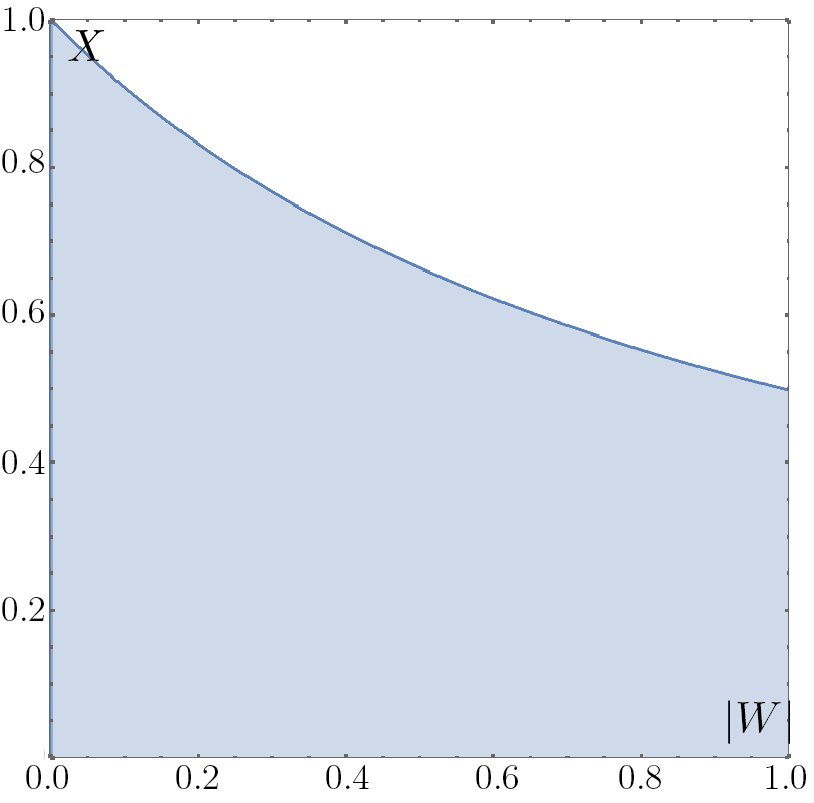
Figure 4: The region of existence of the CDW half-metal. The asymmetric solution of (93) exists in the shaded (blue) area. When dimensionless doping exceeds the critical value $X_{c}$, the consistency relation (92) is violated, inmplying the disappearance of the half-metallic phase. The curve $X_{c}=X_{c}(|W|)$ is parametrically determined by Eq. (94). Asymptotically, at $|W|\gg 1$, it becomes a simple hyperbola $X=|W|^{-1}$.

Next we assume that sector $\sigma$ is empty, while sector $\bar{\sigma}$ is doped. In terms of dimensionless variables this implies the following consistency condition $\delta_{\sigma}>\nu>\delta_{\bar{\sigma}}$. It can be expressed, with the help of (86), as

$$\delta_{\sigma}>\sqrt{\delta_{\bar{\sigma}}^{2}+X^{2}}.$$ (92)

In turn, Eq. (87) allows us to derive

$$\begin{split}\ln[X+\sqrt{X^{2}+\delta_{\bar{\sigma}}^{2}}]&=|W|\Big{(}\frac{\delta_{\sigma}}{\delta_{\bar{\sigma}}}-1\Big{)},\\ \ln\delta_{\sigma}&=|W|\Big{(}\frac{\delta_{\bar{\sigma}}}{\delta_{\sigma}}-1\Big{)}.\end{split}$$ (93)

This is a system of coupled transcendental equations, which must be solved with respect to unknown $\delta$’s at fixed $X$.

While we do not know an analytical solution of this system, and ultimately resort to numerical calculations, some properties of the solution can be found out analytically. Of particular importance is the critical value of doping $X_{c}=X_{c}(|W|)$ above which Eqs. (93) have no solution consistent with inequality (92). Introducing the parameter $s=\delta_{\bar{\sigma}}/\delta_{\sigma}$ we immediately obtain the resultant parametric equations

$$\begin{split}X_{c}(s)&=\frac{\sqrt{1-s^{2}}}{(1+\sqrt{1-s^{2}})^{\frac{s}{s+1}}},\\ |W(s)|&=\frac{s}{1-s^{2}}\ln[1+\sqrt{1-s^{2}}].\end{split}$$ (94)

At the $(|W|,X)$-plane they specify a curve parameterized by variable $s\in[0,1]$. It is shown in Fig. 4, as a line limiting the area, where the solution exists. We see that, at $|W|=0$, sector $\sigma$ remains empty for the doping level as high as $X_{c}(0)=1$. For growing $|W|$, however, the dimensionless critical doping $X_{c}(|W|)$ decreases.

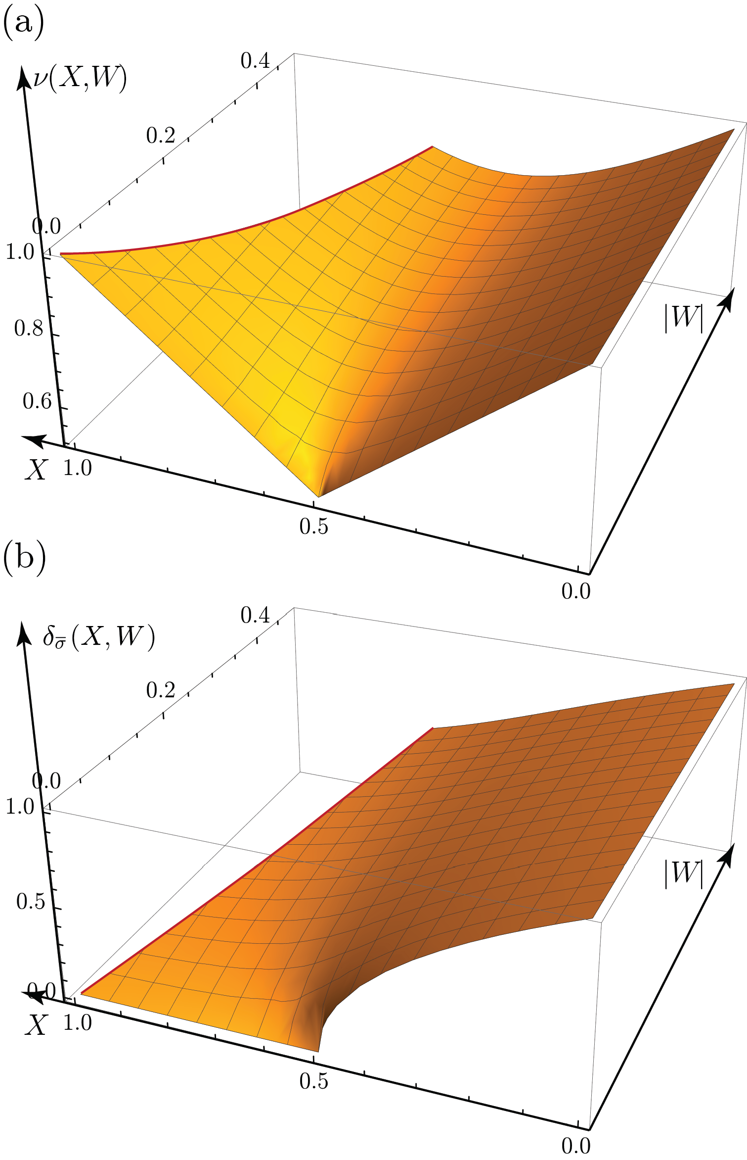
Figure 5: (a) Dimensionless chemical potential as a function of dimensionless particle number $X$ and coupling constant $W$ for the asymmetric CDW state. Only the ${\bar{\sigma}}$ sector is doped. The corner-like shape $\nu=1/2+|X-1/2|$ is clearly pronounced at zero coupling $W=0$. (b) Dimensionless order parameter $\delta_{\bar{\sigma}}$ as a function of the same parameters. A simple solution of system  (93) is clearly evident at $W=0$, where $\delta_{\bar{\sigma}}=\sqrt{1-2X},\ X<1/2$, and the gap closes ($\delta_{\bar{\sigma}}=0$), at $X>1/2$.

Solving the self-consistency conditions numerically, we find both $\delta$’s and $\nu$. Surface in Fig. 5 shows the behavior of $\nu$ as a function of $X$ and $|W|$. We see, that at $|W|=0$, the $\nu=\nu(X)$ dependence exhibits a distinct corner shape, as indeed expected.

Having calculated the chemical potential $\nu(X,W)$, we may now compute the free energy difference for the asymmetric state

$$\frac{F_{\rm A}}{V}=\frac{F_{0}}{V}+N_{\rm F}D_{0}^{2}\int_{0}^{X}\nu(X^{\prime},W)dX^{\prime}.$$ (95)

This formula is analogous to Eq. (52). Unlike the SDW result, however, we evaluate Eq. (95) numerically.

IV.3 Properties of doped CDW phases

Let us compare the free energies of the symmetric and asymmetric phases, see Eqs. (91) and (95). The corresponding plot is presented in Fig. 6. Our calculations demonstrate that, if the asymmetric phase exists, it always has lower energy than the symmetric phase. In other words, for $X\in[0,X_{c}(|W|)]$, the model ground state is the asymmetric phase.

For higher doping, the asymmetric phase is impossible. Hence, the curve $X=X_{c}(W)$ is the transition line separating two phases (symmetric and asymmetric). Since the doping in a specific sector changes discontinuously upon transition between symmetric and asymmetric states, we conclude that the transition is the first order one (discontinuous).

In the $X_{c}<X<1$ range, the symmetric solution is realized. For even higher doping $X>1$, the order parameter is completely suppressed, and the system is a metal with no broken symmetries.

There are several similarities between the symmetric and asymmetric phases. Both of them are characterized by a finite CDW order parameter. For the symmetric phase, we can write a concise formula for this order parameter

$$|\Delta|=\frac{2g}{g-2\bar{g}_{\bot}}D_{0}\sqrt{1-\frac{\gamma x}{2N_{\rm F}D_{0}}}.$$ (96)

For the asymmetric phase, a simple analytical expression valid at arbitrary $X$ is unknown to us. Further, both phases are metallic, with well-developed Fermi surfaces, which are two concentric spheres. The radii of these spheres are determined by Eq. (37), in which $\Delta_{\sigma}$ must be replaced by $D_{\sigma}$.

Yet, there are important distinctions between the two. In regard to their metallicity, one must remember that, while the symmetric phase is a kind of a paramagnetic metal, the asymmetric phase is a half-metal: its sector $\bar{\sigma}$ has no Fermi surface.

In addition, the asymmetry in doping implies finite ferromagnetic polarization: all fermions introduced by the doping enter sector $\sigma$, where all single-fermion states have spin projection $\sigma$. Consequently, the total spin polarization is $x$. Quite remarkably, the asymmetric phase has a finite SDW polarization $\propto(D_{\uparrow}-D_{\downarrow})\cos({\bf Q}\cdot{\bf r}+\phi)$. Thus, the total spin polarization is equal to

$$\langle S_{z}({\bf r})\rangle=x+2g^{-1}(D_{\uparrow}-D_{\downarrow})\cos({\bf Q}\cdot{\bf r}+\phi),$$ (97)

Here, $\phi$ is an arbitrary constant determined by the origin in the $\mathbf{r}$ space. One can check directly that $\langle S_{z}({\bf r})\rangle\equiv 0$ in the symmetric state.

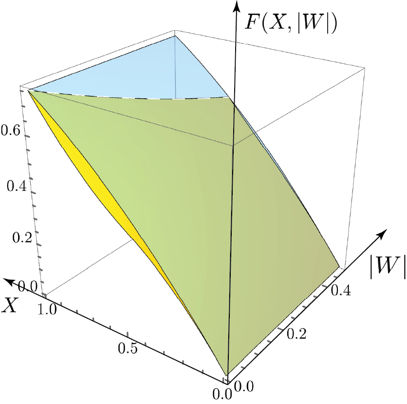
Figure 6: Free energy of the symmetric (blue semitransparent surface) and asymmetric (yellow surface) states of the model as a function of the dimensionless particle number $X$ and coupling constant $|W|$. One clearly sees that asymmetric phase is energetically favorable in the entire region, where it exists. Exactly at the critical doping $X_{c}(X)$ (the dashed curve, see also Fig. 4 and Eq. 94), both the symmetric and asymmetric phases yave the same energy. At $X>X_{c}$, the symmetric phase prevails.

Let us address the situation, for which the solution of the asymmetric system (93) disappears. This occurs precisely, when condition (92) breaks. That is, the particle number attains a critical value $X_{c}=X(W)$ such that it cannot be accommodated in a single band pocket (see Fig. 4). That corresponds to the limiting relation between the gaps

$$\delta_{\sigma}^{2}=X_{c}^{2}+\delta_{\bar{\sigma}}^{2},\quad\nu=\sqrt{\delta_{\bar{\sigma}}^{2}+X_{c}^{2}}.$$ (98)

As doping grows beyond the critical value, the state changes to the symmetric one $X_{\sigma}=X_{-\sigma}\equiv X/2$. This also implies that

$$\delta_{\sigma}=\delta_{\bar{\sigma}},\quad\nu=\sqrt{\delta_{\bar{\sigma}}^{2}+X^{2}/4}.$$ (99)

In other words, the gaps and partial dopings in both sectors are identical. The transition between asymmetric and symmetric phases is discontinuous (of the first order).

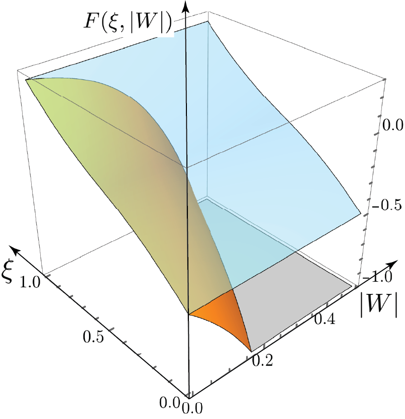
Figure 7: The free energy of the CDW (orange) vs SDW (blue) phases for the negative values of $W$ as a function of dimensionless particle number $\xi$ and $|W|$. We see that for all relevant parameter values, the CDW state has the lowest energy. The degeneracy of the free energy of SDW and CDW at $W=0$ is pronounced. The gray surface is a clipping plane.

V Phase diagram of the model

Our analysis has demonstrated that the ground state of the model depends on doping $x$. Another important parameter affecting the ground state is $\bar{g}_{\bot}$: it controls the switching between the SDW and CDW orders, and, within the CDW phase, it affects the strength of the order parameter. In this section, we construct the model’s phase diagram that summarizes these trends in a single layout.

Of course, it is convenient to use dimensionless variables instead of $x$ and $\bar{g}_{\bot}$. For example, we can use $\bar{g}_{\bot}/g$ or $W$ as a dimensionless representation of $\bar{g}_{\bot}$. However, dimensionless $X_{\sigma}$ is not very suitable for this purpose, since its very definition, see Eq. (85), contains $\bar{g}_{\bot}$. To circumvent this issue, let us introduce new dimensionless quantities

$$\xi_{\sigma}=\frac{\gamma x_{\sigma}}{2N_{\rm F}\Delta_{0}},\quad\xi=\sum_{\sigma}\xi_{\sigma}.$$ (100)

Note that $X=\xi e^{2W}$.

V.1 SDW order

To construct the phase diagram, we need to compare the free energies of all phases we have identified. Let us start with the SDW ordering. We know that, for low doping, $x<N_{\rm F}\Delta_{0}/\gamma$, the free energy of the SDW state is expressed by Eq. (52). Exactly at $x=N_{\rm F}\Delta_{0}/\gamma$, the order parameter $\Delta_{\sigma}$ at the sector hosting all doped charge carriers vanishes, $\Delta_{\sigma}=0$, and remains to be empty for larger $x$.

This nullification of $\Delta_{\sigma}$ manifests itself as a second-order transition between two types of the SFHM. Both these phases correspond to asymmetric state, both are half-metals. The energy of the high-doping SFHM is $F_{\rm A}=-N_{\rm F}\Delta_{0}^{2}/2+\gamma^{2}x^{2}/(4N_{\rm F})$, for $x>N_{\rm F}\Delta_{0}/\gamma$. We can express the free energy for the SDW ordering as follows

$$F_{\rm sdw}(\xi)/V=N_{\rm F}\Delta_{0}^{2}\begin{cases}-1+2\xi-\xi^{2},\quad\xi\leqslant\frac{1}{2},\\ \xi^{2}-\frac{1}{2},\quad\xi>\frac{1}{2}.\end{cases}$$ (101)

V.2 CDW order

At $X<X_{c}$, the free energy of the CDW state in the same notation reads

$$F_{\rm cdw}(\xi)/V=N_{\rm F}\Delta_{0}^{2}e^{-4W}\!\left[-1\!+\!2\!\int_{0}^{\xi e^{2W}}\!\!\!\nu(X)\,dX\right]\!\!.$$ (102)

This expression must be evaluated numerically.

Let us recall that, at $X=X_{c}$, within the CDW order, there is a phase transition between symmetric and asymmetric states. The first-order transition line separating these states is specified by parametric equations (94). In terms of $\xi$ and $\bar{g}_{\bot}/g$ variables, we can rewrite these formulas as

$$\begin{split}\xi(s)&\equiv\xi_{1}(s)=\sqrt{1-s^{2}}(1+\sqrt{1-s^{2}})^{\frac{s}{1-s}},\\ \frac{\bar{g}_{\bot}}{g}&=-\frac{gN_{\rm F}|W(s)|}{1-2gN_{\rm F}|W(s)|}.\end{split}$$ (103)

When $\bar{g}=0$, or, equivalently, $W=0$, it is trivial to check that $\xi_{1}=1$. In the opposite limit, at $\bar{g}_{\bot}\gg g$, we have $|W|\rightarrow 1/(2N_{\rm F}g)$ and $\xi_{1}\rightarrow\exp(2|W|)/|W|$.

The symmetric CDW order disappears completely at $X=1$, see Eqs. (89) and (90). This condition defines a second-order transition line

$$\xi_{2}(W)=e^{2|W|}$$ (104)

that separates a normal metal and a metal with the CDW order parameter. Here, $W$ as a function of $\bar{g}_{\bot}/g$ is given by Eq. (103).

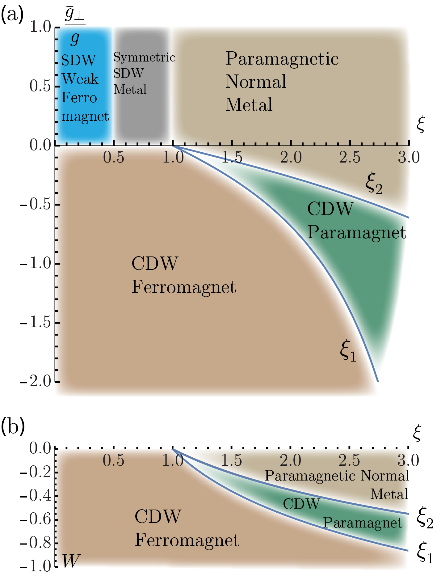
Figure 8: Phase diagram. (a) $\xi=\gamma x/(2N_{\rm F}\Delta_{0})$ is the dimensionless particle number. Curve $\xi_{1}$ ($\xi_{2}$) is expressed by Eq. (103) [Eq. (104)] We used $gN_{\rm F}=0.5$ for definiteness. Curve $\xi_{1}$ becomes vertical at $\xi\rightarrow\exp(1/gN_{\rm F})$. (b) The phase diagram presented in universal units (independent of the coupling parameter $gN_{\rm F}$) $W$ and $\xi$ for negative values of $W$. Here, both curves have exponential asymptotic behavior $\xi_{1}(W)\rightarrow\exp(2|W|)/|W|$, while $\xi_{2}(W)$ is given by Eq. 104 at large $W$.

V.3 Phase diagram details

The resultant phase diagram is shown in Fig. 8. Comparing $F_{\rm sdw}$ and $F_{\rm cdw}$, we find that, at $W<0$, the CDW always has the lowest energy, see Fig. 7. As a result, at any negative $\bar{g}_{\bot}$ the CDW phase prevails for any doping.

We see that at $\bar{g}_{\bot}<0$ (at $\bar{g}_{\bot}>0$) the CDW (the SDW) prevails. This feature can be interpreted as follows: the effective $\bar{g}_{\bot}$ becomes negative only when the charge carriers interact with the lattice, and the latter is sufficiently soft. Otherwise, the exchange interaction makes the CDW either metastable, or unstable.

On crossing the line $\bar{g}_{\bot}=0$, $\xi\in[0,1]$, the system demonstrates the first-order transition between the CDW and the SDW orders. Specifically, the ferromagnetic magnetization experiences a discontinuity at this transition, as one can prove comparing Eqs. (59) and (97).

As we have seen in Sec. III, the coupling constant $\bar{g}_{\bot}$ does not affect the SDW phase. That is why all phase boundaries in the SDW phase are vertical straight lines. The $\xi\in[0,1],\ W>0$ strip is split into two halves by $\xi=0.5$ line separating the asymmetric and symmetric SDW phases. Boundary value $\xi=0.5$ corresponds to a critical doping level $x=N_{\rm F}\Delta_{0}/\gamma$ (see Eq.  (100)) where the number of particles is too high to accomodate all of them in a single sector of the SDW state (cf. Eq. (45)).

At $\bar{g}_{\bot}=0$, $\xi=0.5$, there is a tricritical point where two SFHM phases meet the CDW half-metal. Examining this point, one may wonder why there is no second type of the CDW half-metal, similar to the second type of the SFHM. To answer this question, let us recall the difference between two SFHM’s: the low-doping SFHM ($0<\xi<0.5$) has finite order parameter in the sector hosting the inserted carriers, while for the high-doping SFHM ($0.5<\xi<1$) this order parameter is zero. Such a situation is mathematically forbidden for the CDW half-metal: Eqs. (93) have no non-trivial solution for which $\delta_{\sigma}=0$. In other words, because of the intersector coupling in the CDW phase, the empty-sector order parameter does not allow the nullification of the filled-sector order parameter. One can treat $\delta_{\bar{\sigma}}$ as a kind of external field for $\delta_{\sigma}$, whose presence replaces the second-order transition by a crossover.

At $\bar{g}_{\bot}=0$ and $\xi=1$, we see a tetracritical point: the CDW half-metal, the CDW paramagnet, the SFHM, and normal metal phases coexist there. Of four transition lines meeting at this point, only one corresponds to the second-order transition: the CDW paramagnet order parameters smoothly vanish at the transition to the normal metal, see Eq. (89). Three other lines represent discontinuous transitions: for example, one can check that, on crossing any of these lines, the ferromagnetic magnetization demonstrates a discontinuity.

VI Discussion

VI.1 Results and approximations overview

Our investigation of the model revealed several ordered states that are sensitive to the doping and interaction structure. We studied magnetic and metallic properties of these phase and mapped out the phase diagram.

All doped phases on the phase diagram are metallic, with well-developed Fermi surface. Except for the CDW paramagnet and normal metal, all other doped phases are ferromagnetic half-metals, with non-trivial spatially modulated spin textures. The latter circumstance is particularly surprising in case of the CDW ordered phases: a gappped nonmagnetic insulator acquires a ferromagnetic polarization, coexisting with a SDW-like spin order, see Eq. (97).

To assess the validity of these findings, we must also remember the assumptions that we made in our study, as well as propose possible enhancements for the model. First of all, all our calculations were performed at $T=0$. Generalization beyond this limit is a matter of the future research.

Further, we employed the mean field approximation. We believe that for a three-dimensional many-fermion system (and, perhaps, for a two-dimensional system at $T=0$) currently,t there is no known mechanism that would qualitatively alter any mean field conclusion, as long as coupling constants are weak. A brief overview of recent literature relevant for this issue can be found in Appendix A of Ref. Kokanova et al., 2021.

From the very beginning of our investigation, we assumed that no macroscopic phase separation is allowed: apart from density modulations with the CDW wave vector ${\bf Q}$, the density is postulated to be the same everywhere. For this to be true, the long-range Coulomb interaction must be sufficiently strong. A detailed exploration of the Coulomb interaction role is an interesting direction for future studies.

Our density-waves order parameters are characterized by the nesting wave vector ${\bf Q}$. In our calculations it was always treated as an invariable quantity. Nonetheless, it is possible to view ${\bf Q}$ as yet another minimization parameter. Suitable formalism is quite old, see Ref. Rice, 1970. It is straightforward but cumbersome. At the same time, the energy gain due to minimization over ${\bf Q}$ is quite insignificant. Thus, we chose to disregard this possibility. As a justification, one can imagine that ${\bf Q}$ is commensurate with the lattice, thus, its value is pinned by the lattice. Possible ${\bf Q}$ incommensurability opens yet another direction, in which this research can be extended: the role of the umklapp interaction.

The electron-lattice coupling is an important element of our model. Thanks to this interaction, the CDW can win the competition against the SDW phase (the SDW is typically stronger without the lattice participation due to the exchange interaction disfavoring the CDW). Since the crystal lattice plays a rather minor role, it was accounted for within a very minimalist framework: a single mode, treated as static non-quantum variable $\varphi_{\mathbf{Q}}$. In principle, more realistic description of the lattice may be included into the model.

VI.2 Stoner mechanism of ferromagnetism

As we explained in the Introduction, the mechanism discussed in this paper is unrelated to the Stoner instability. To prove this, let us recall that the latter implies that a many-fermion system enters a ferromagnetic phase when the inequality

$$gN_{\rm F}>1$$ (105)

becomes valid. Since our model is in the weak-coupling limit, this relation is definitely violated.

The weak-coupling limit, which we confined ourselves to, should be seen as an important theoretical advantage: when coupling constants are small, the mean field results can be consistently tested with the help of a suitably designed perturbative expansion. This possibility is to be contrasted with the Stoner criterion framework. Simplicity and universality of Eq. (105) creates an impression of an easy-to-use multipurpose tool, applicable for lattice as well as continuum models. Unfortunately, the reliability of Eq. (105) as a predictor of a ferromagnetic phase is not beyond reproach. Clearly, for the Stoner instability to occur, a system must enter intermediate or strong coupling limit. The arsenal of analytical instruments that are available in these regimes is severely restricted. Moreover, no controlled derivation of condition Eq. (105) is known.

This brings numerical approaches to the forefront of research efforts. In this regard, there is ample numerical evidence questioning trustworthiness of condition (105). Specifically, recent computational works Drummond and Needs (2009); Holzmann and Moroni (2020); Azadi and Drummond (2022) indicated that the Stoner ferromagnetism is likely to be never a ground state of the jellium model of electron gas. Likewise, the Monte Carlo simulations for ³He Taddei et al. (2015); Holzmann et al. (2006) found no ferromagnetic phase, in agreement with experimentally known phase diagram of ³He.

Application of the Stoner criterion to a Hubbard-like Hamiltonian may be inconsistent with numerical data as well, as the authors of Ref. Arovas et al., 2022 argued. The presence of a ferromagnetic state at the phase diagram of a triangular lattice model has been discussed in a recent publication Morera and Demler (2024), yet the relevance of the Stoner mechanism to this phase is not immediately clear.

In the realm of experimental physics, the guidance provided by the inequality (105) may be quite unreliable as well. Consider, for example, liquid ³He. The interaction between He atoms is typically modeled by the hard-sphere potential, implying that $g$ in Eq. (105) is extremely large. Yet, no liquid ferromagnetic phase of ³He is known. Also, we can recall how early optimistic papers Vitkalov et al. (2001); Shashkin et al. (2001) reporting ferromagnetism observation in silicon MOSFET were later criticized Pudalov et al. (2002) for data interpretation being too one-sided. Likewise, recent review paper Shashkin and Kravchenko (2019), while acknowledging the contribution of Refs. Vitkalov et al., 2001; Shashkin et al., 2001 to the field, did not endorse the Stoner-ferromagnetism interpretation.

Speaking more broadly, the Stoner proposal ignores various correlation effects that affect the energies of both polarized and paramagnetic liquids. In lattice models, with their assortment of ordered states, competition with other phases may additionally impede ferromagnetism stabilization. (To appreciate the latter issue, one may examine phase diagrams in Ref. Igoshev et al., 2015 that compare blanket Stoner criterion prediction with rich phase diagrams obtained within either slave-boson or Hartree-Fock approximations.) These rather common features of many-fermion models make simple and universal prescription (105) quite unreliable in many important situations. Therefore, while the Stoner criterion remains a popular research tool even today, the associated issues must not be overlooked.

Despite these problems, it is difficult to ignore the fact that the Bloch-Stoner calculations were one of the first quantum-mechanical many-body theories, a pioneering attempt to derive a consistent explanation of an ordered many-electron state in condensed matter. Ultimately, it is hardly a surprise that over many decades of research our understanding of solid state magnetism has evolved, motivating re-examination of previous concepts.

VI.3 Possible realizations of the model: graphene multilayers

In connection with possible realization of our model in experiment, it is necessary to remember that the ingredients required by our proposal are not that unique. There are, indeed, substantial variety of materials demonstrating nesting-driven SDW or CDW phases (although we assumed spherical Fermi surfaces, this is mostly a matter of convenience, and any type of nested Fermi surface suits us). If these can be doped, the stabilization of a ferromagnetic state becomes an option.

Being more specific, we would like to mention the so-called fractional metal states in graphene-based materials. The fractional metals can be conceptualized as a generalization of ferromagnetic phase for a system with both spin and valley degeneracies. These states have been theoretically predicted in Ref. Sboychakov et al., 2021; Rakhmanov et al., 2023. Experimental observations have been reported in Ref. Zhou et al., 2021, 2022.

To establish their relevance for our model, let us observe that graphene bilayers demonstrate an instability toward an insulating ordered state Rozhkov et al. (2016). The instability is driven either by nesting (for AA-stacking), or by quadratic band touching (for AB-staking). Depending on details, doped system may demonstrate either spatially inhomogeneous state, or, instead, polarization in terms of valley and spin-related indices, similar to the behavior discussed in subsection III.2. Additional details can be found in Refs. Sboychakov et al., 2021; Rakhmanov et al., 2023.

VII Conclusions

Using the mean field approximation, we investigated a model with electrons and holes whose Fermi surfaces are perfectly nested. It was assumed that the fermions interact with each other and with the lattice. All interactions are weak. To suppress inhomogeneous states, strong long-range Coulomb repulsion was included into the model. When undoped, the ground state of such a model is insulating and demonstrates a density-wave order, either SDW, or CDW. The doping weakens both types of order. Additionally, finite ferromagnetic polarization emerges. We constructed the phase diagram of the model, and studied various properties of the ordered phases.

References

- Bloch (1929) F. Bloch, “Bemerkung zur Elektronentheorie des Ferromagnetismus und der elektrischen Leitfähigkeit,” Z. Phys. 57, 545 (1929).
- Stoner (1938) E. C. Stoner, “Collective electron ferromagnetism,” Proc. R. Soc. Lond. 165, 372 (1938).
- Huang (1987) K. Huang, Statistical mechanics (John Wiley & Sons, 1987).
- Blundell (2001) S. Blundell, Magnetism in condensed matter (Oxford University Press, Oxford, 2001).
- Zhou et al. (2021) H. Zhou, T. Xie, A. Ghazaryan, T. Holder, J. R. Ehrets, E. M. Spanton, T. Taniguchi, K. Watanabe, E. Berg, M. Serbyn, et al., “Half- and quarter-metals in rhombohedral trilayer graphene,” Nature 598, 429 (2021).
- Raines et al. (2024) Z. M. Raines, L. I. Glazman, and A. V. Chubukov, “Unconventional Discontinuous Transitions in Isospin Systems,” Phys. Rev. Lett. 133, 146501 (2024).
- Mohanta and Mishra (2017) S. Mohanta and S. Mishra, “Electronic structure and magnetic moment of dilute transition metal impurities in semi-metallic CaB6,” J. Magn. Magn. Mater. 444, 349 (2017).
- Holzmann and Moroni (2020) M. Holzmann and S. Moroni, “Itinerant-Electron Magnetism: The Importance of Many-Body Correlations,” Phys. Rev. Lett. 124, 206404 (2020).
- Rozhkov et al. (2017) A. V. Rozhkov, A. L. Rakhmanov, A. O. Sboychakov, K. I. Kugel, and F. Nori, “Spin-Valley Half-Metal as a Prospective Material for Spin Valleytronics,” Phys. Rev. Lett. 119, 107601 (2017).
- Rakhmanov et al. (2018) A. L. Rakhmanov, A. O. Sboychakov, K. I. Kugel, A. V. Rozhkov, and F. Nori, “Spin-valley half-metal in systems with Fermi surface nesting,” Phys. Rev. B 98, 155141 (2018).
- Abrikosov et al. (1975) A. A. Abrikosov, L. P. Gorkov, and I. E. Dzyaloshinski, Methods of Quantum Field Theory in Statistical Physics (Dover, New York, 1975).
- Gorbatsevich et al. (1992) A. Gorbatsevich, V. Kopaev, and I. Tokatly, “Band theory of phase stratification,” Sov. Phys. JETP 74, 521 (1992).
- Gor’kov and Teitel’baum (2010) L. P. Gor’kov and G. B. Teitel’baum, “Spatial inhomogeneities in iron pnictide superconductors: The formation of charge stripes,” Phys. Rev. B 82, 020510 (2010).
- Igoshev et al. (2010) P. A. Igoshev, M. A. Timirgazin, A. A. Katanin, A. K. Arzhnikov, and V. Y. Irkhin, “Incommensurate magnetic order and phase separation in the two-dimensional Hubbard model with nearest- and next-nearest-neighbor hopping,” Phys. Rev. B 81, 094407 (2010).
- Igoshev et al. (2015) P. A. Igoshev, M. A. Timirgazin, V. F. Gilmutdinov, A. K. Arzhnikov, and V. Y. Irkhin, “Spiral magnetism in the single-band Hubbard model: the Hartree–Fock and slave-boson approaches,” J. Phys.: Condens. Matter 27, 446002 (2015).
- Rakhmanov et al. (2017) A. L. Rakhmanov, K. I. Kugel, M. Y. Kagan, A. V. Rozhkov, and A. O. Sboychakov, “Inhomogeneous electron states in the systems with imperfect nesting,” JETP Lett. 105, 806 (2017).
- Rakhmanov et al. (2020) A. L. Rakhmanov, K. I. Kugel, and A. O. Sboychakov, “Coexistence of spin density wave and metallic phases under pressure,” J. Supercond. Novel Magn. 33, 2405–2413 (2020).
- Kokanova et al. (2021) S. V. Kokanova, P. A. Maksimov, A. V. Rozhkov, and A. O. Sboychakov, “Competition of spatially inhomogeneous phases in systems with nesting-driven spin-density wave state,” Phys. Rev. B 104, 075110 (2021).
- M. Yu. Kagan et al. (2021) M. Yu. Kagan, K. I. Kugel, and A. L. Rakhmanov, “Electronic phase separation: Recent progress in the old problem,” Phys. Rep. 916, 1 (2021).
- M. Yu. Kagan et al. (2024) M. Yu. Kagan, K. I. Kugel, A. L. Rakhmanov, and A. O. Sboychakov, Electronic phase separation in magnetic and superconducting materials: Recent advances, vol. 201 of Springer Series in Solid-State Sciences (Springer Switzerland, 2024).
- Khokhlov et al. (2020) D. A. Khokhlov, A. L. Rakhmanov, A. V. Rozhkov, and A. O. Sboychakov, “Dynamical spin susceptibility of a spin-valley half-metal,” Phys. Rev. B 101, 235141 (2020).
- Sboychakov et al. (2020) A. O. Sboychakov, A. V. Rozhkov, K. I. Kugel, and A. L. Rakhmanov, “Phase separation in a spin density wave state of twisted bilayer graphene,” JETP Lett. 112, 651 (2020).
- Sboychakov et al. (2021) A. O. Sboychakov, A. L. Rakhmanov, A. V. Rozhkov, and F. Nori, “Bilayer graphene can become a fractional metal,” Phys. Rev. B 103, L081106 (2021).
- Rakhmanov et al. (2023) A. L. Rakhmanov, A. V. Rozhkov, A. O. Sboychakov, and F. Nori, “Half-metal and other fractional metal phases in doped bilayer graphene,” Phys. Rev. B 107, 155112 (2023).
- de Groot et al. (1983) R. A. de Groot, F. M. Mueller, P. G. van Engen, and K. H. J. Buschow, “New Class of Materials: Half-Metallic Ferromagnets,” Phys. Rev. Lett. 50, 2024 (1983).
- Rice (1970) T. M. Rice, “Band-Structure Effects in Itinerant Antiferromagnetism,” Phys. Rev. B 2, 3619 (1970).
- Drummond and Needs (2009) N. D. Drummond and R. J. Needs, “Phase Diagram of the Low-Density Two-Dimensional Homogeneous Electron Gas,” Phys. Rev. Lett. 102, 126402 (2009).
- Azadi and Drummond (2022) S. Azadi and N. D. Drummond, “Low-density phase diagram of the three-dimensional electron gas,” Phys. Rev. B 105, 245135 (2022).
- Taddei et al. (2015) M. Taddei, M. Ruggeri, S. Moroni, and M. Holzmann, “Iterative backflow renormalization procedure for many-body ground-state wave functions of strongly interacting normal Fermi liquids,” Phys. Rev. B 91, 115106 (2015).
- Holzmann et al. (2006) M. Holzmann, B. Bernu, and D. M. Ceperley, “Many-body wavefunctions for normal liquid ,” Phys. Rev. B 74, 104510 (2006).
- Arovas et al. (2022) D. P. Arovas, E. Berg, S. A. Kivelson, and S. Raghu, “The Hubbard Model,” Annu. Rev. Condens. Matter Phys. 13, 239 (2022).
- Morera and Demler (2024) I. Morera and E. Demler, “Itinerant magnetism and magnetic polarons in the triangular lattice Hubbard model,” (2024), eprint arXiv:2402.14074.
- Vitkalov et al. (2001) S. A. Vitkalov, H. Zheng, K. M. Mertes, M. P. Sarachik, and T. M. Klapwijk, “Scaling of the Magnetoconductivity of Silicon MOSFETs: Evidence for a Quantum Phase Transition in Two Dimensions,” Phys. Rev. Lett. 87, 086401 (2001).
- Shashkin et al. (2001) A. A. Shashkin, S. V. Kravchenko, V. T. Dolgopolov, and T. M. Klapwijk, “Indication of the Ferromagnetic Instability in a Dilute Two-Dimensional Electron System,” Phys. Rev. Lett. 87, 086801 (2001).
- Pudalov et al. (2002) V. Pudalov, M. Gershenson, H. Kojima, N. Butch, E. Dizhur, G. Brunthaler, A. Prinz, and G. Bauer, “Low-density spin susceptibility and effective mass of mobile electrons in Si inversion layers,” Phys. Rev. Lett. 88, 196404 (2002).
- Shashkin and Kravchenko (2019) A. A. Shashkin and S. V. Kravchenko, “Recent developments in the field of the metal-insulator transition in two dimensions,” Appl. Sci. 9, 1169 (2019).
- Zhou et al. (2022) H. Zhou, L. Holleis, Y. Saito, L. Cohen, W. Huynh, C. L. Patterson, F. Yang, T. Taniguchi, K. Watanabe, and A. F. Young, “Isospin magnetism and spin-polarized superconductivity in Bernal bilayer graphene,” Science 375, 774 (2022).
- Rozhkov et al. (2016) A. Rozhkov, A. Sboychakov, A. Rakhmanov, and F. Nori, “Electronic properties of graphene-based bilayer systems,” Phys. Rep. 648, 1 (2016).