Synthetic Tabular Data Generation: A Comparative Survey for Modern Techniques

Abstract.

As privacy regulations become more stringent and access to real-world data becomes increasingly constrained, synthetic data generation has emerged as a vital solution, especially for tabular datasets, which are central to domains like finance, healthcare and the social sciences. This survey presents a comprehensive and focused review of recent advances in synthetic tabular data generation, emphasizing methods that preserve complex feature relationships, maintain statistical fidelity, and satisfy privacy requirements. A key contribution of this work is the introduction of a novel taxonomy based on practical generation objectives, including intended downstream applications, privacy guarantees, and data utility, directly informing methodological design and evaluation strategies. Therefore, this review prioritizes the actionable goals that drive synthetic data creation, including conditional generation and risk-sensitive modeling. Additionally, the survey proposes a benchmark framework to align technical innovation with real-world demands. By bridging theoretical foundations with practical deployment, this work serves as both a roadmap for future research and a guide for implementing synthetic tabular data in privacy-critical environments.

1. Introduction

The increasing reliance on data-driven technologies across sectors such as finance (Tian et al., 2021), healthcare (Rahman et al., 2023), marketing (Arthur, 2013), and social sciences (Zhang et al., 2020) highlights the critical role of large, representative datasets in fostering innovation. For instance, big data analytics in finance has transformed investment strategies (Vishweswar Sastry et al., 2024), while large datasets in healthcare have advanced personalized medicine and predictive analytics (Clim et al., 2019). However, the collection, storage, and sharing of real-world data face significant challenges, including privacy, regulatory compliance, data scarcity, and logistical difficulties (Zhao and Zhang, 2019). These challenges have led to the development of synthetic data generation techniques, which create artificial datasets that replicate the properties of real-world data while protecting sensitive information.

The demand for synthetic data (Lu et al., 2023) arises from the limited accessibility of high-quality datasets, particularly due to strict privacy regulations like General Data Protection Regulation (GDPR) (European Union, 2016) and The Health Insurance Portability and Accountability Act (HIPAA) (of Health and Services, 1996). Synthetic data enables the creation of anonymized datasets, facilitating collaboration and promoting data democratization (Amplitude, 2024; Lu et al., 2023). Additionally, it addresses issues of data imbalance in fields like fraud detection and medical research, enhancing model accuracy and generalizability (He and Garcia, 2009) Synthetic data generation also offers a cost-effective alternative to real-world data collection (Babbar and Schölkopf, 2019), which is often expensive and time-consuming. Once trained, models can produce vast amounts of data at a fraction of the cost, making them scalable for organizations with limited resources.

Past decade, synthetic data generation has achieved remarkable success across diverse domains, despite several challenges. Capturing complex data distributions, preserving privacy, maintaining feature dependencies, and balancing realism with diversity have all posed significant hurdles. Recent advancements in generative models, such as Generative Adversarial Networks (GANs) (Goodfellow et al., 2014) and Variational Autoencoders (VAEs) (Kingma and Welling, 2013), have been pivotal in overcoming these hurdles, enabling the creation of synthetic data that better mirrors real-world datasets while addressing privacy concerns and enhancing utility. GANs excel in creating high-quality images and text, while VAEs are particularly suited for probabilistic data generation. These innovations have enabled transformative applications across several industries. In finance, synthetic data is leveraged for fraud detection (Assefa et al., 2020), simulating market conditions, and testing trading algorithms, all without financial risk. In computer vision (Karras et al., 2019), GANs (Goodfellow et al., 2014) generate photorealistic images for data augmentation. In healthcare (Hernandez et al., 2022), synthetic patient records support research in privacy-sensitive scenarios with limited real-world data. Similarly, synthetic data plays a crucial role in training autonomous vehicles (Dosovitskiy et al., 2017) by simulating diverse driving environments, ensuring robust and safe performance.

While synthetic data generation techniques have been successful for various data types such as images, text, audio, video and time series, tabular data presents unique challenges and opportunities that warrant focused attention. Unlike unstructured data (e.g., images or text), tabular data is characterized by heterogeneous feature types (e.g., numerical, categorical, and ordinal), complex inter-feature dependencies, and domain-specific constraints. Particularly in financial domains (Assefa et al., 2020), for instance, institutions must balance data utility and privacy when developing models for CreditRisk assessment (Kaggle, nd), fraud detection, and loan approvals. Sharing real transaction data can lead to privacy breaches and regulatory violations, thus making synthetic data a viable alternative. However, generating synthetic tabular data requires preserving intricate feature relationships (e.g., correlations between income, credit score, and loan repayment behavior) while ensuring privacy and statistical fidelity. These challenges are less pronounced in other data types, where the focus is often on preserving structural patterns (e.g., pixel relationships in images or semantic coherence in text).

This survey examines key advancements, challenges, and real-world applications for effective tabular synthetic data generation, providing actionable insights for researchers and practitioners. Unlike (Figueira and Vaz, 2022), which offers a broad overview of synthetic data generation across all data types with a particular emphasis on GAN-based models and evaluation techniques for privacy and utility, this work focuses specifically on tabular data, emphasizing methods that capture complex feature relationships while ensuring privacy. In contrast to (Lu et al., 2023), which reviews synthetic data generation from a machine learning perspective and categorizes techniques by learning paradigms while highlighting emerging trends and open challenges, our survey prioritizes the objectives that drive synthetic data generation namely, practical purposes and intended downstream uses that determine how synthetic data should be generated and evaluated. While (Bauer et al., 2024) delivers a comprehensive, multidimensional taxonomy of synthetic data generation approaches, covering aspects such as generation goals primarily categorizes existing methods based on broad purposes like data augmentation, data types, and privacy considerations. In contrast, our survey uniquely emphasizes generation objectives as actionable design drivers, detailing how specific intended use cases, including stringent privacy preservation requirements, shape methodological choices, fidelity standards, and evaluation metrics. Unlike these prior works, this 2025 survey introduces a benchmark framework grounded in these objectives to guide the development of synthetic data systems that are not only technically robust but also aligned with targeted real-world needs, including strong privacy guarantees.By bridging theoretical advancements with practical applications, this survey evaluates how different models perform under real-world constraints, particularly in financial risk modeling. The focus on tabular data is justified by its widespread use in critical decision-making processes, the complexity of its feature dependencies, and the pressing need for privacy-preserving solutions in industries like finance, healthcare, and e-commerce.

The survey is structured as follows. Section 2 defines synthetic data generation, providing essential terminology and context. Section  3 focuses on tabular synthetic data generation, categorizing methods based on key characteristics such as feature dependency, statistical preservation, preserving privacy, conditioning on specific attributes and leveraging specific domain knowledge. Section  4 presents benchmarking studies that compare different synthetic data generation models across datasets, highlighting their performance with respect to utility, privacy, and statistical fidelity. Section  5 highlights challenges and limitations. Finally, the Appendices provide foundational background, including definitions, data types, taxonomy related tables anda detailed descriptions of evaluation metrics, ll of which support and complement the discussions in the main sections.

2. Synthetic Data Generation

Synthetic data generation refers to the process of creating artificial data that retains the statistical properties and patterns of real-world datasets (Figueira and Vaz, 2022). It has been explored from multiple perspectives, with key focus on statistical fidelity, feature dependency, and privacy preservation. In this section, we first present definitions from key research works to highlight these perspectives and then synthesize these views to propose a comprehensive definition that aligns with the core objectives of synthetic data generation.

2.1. Definitions

To understand the nuances of synthetic data generation, it is useful to compare how different methods define the process. Table LABEL:tab:synthetic_data_definitions contains examples of synthetic data generation definitions in prior literature, providing a comparative overview of these definitions and highlighting the mathematical formulation underlying synthetic data generation. Existing definitions emphasize the estimation of the original data distribution $P(\mathbf{X})$ and the generation of new synthetic data $\mathbf{X_{\text{syn}}}$ by sampling from an estimated distribution $\hat{P}(\mathbf{X})$. However, different approaches prioritize distinct aspects. For instance, (Bishop and Nasrabadi, 2006) and (Goodfellow et al., 2014) emphasize the need to ensure that $\mathbf{X_{\text{syn}}}$ maintains the statistical properties and feature dependencies of the original dataset. GANs (Goodfellow et al., 2014) achieve this through adversarial learning, while VAEs use latent variable models to structure the data. (Kingma and Welling, 2013) describe conditional synthetic data generation as sampling from $P(\mathbf{X}\mid A=a)$, ensuring that the generated data aligns with specified conditions. Lastly, (Reynolds et al., 2009) and (Goodfellow et al., 2014) discuss how privacy-focused synthetic data methods introduce noise into $\hat{P}(\mathbf{X})$ or the sampling process to prevent re-identification while maintaining data utility. Building on these insights, we formally define synthetic data generation as follows.

Let $\mathbf{X}$ represent the original data, where $\mathbf{X}$ follows a probability distribution $P(\mathbf{X})$. The goal of synthetic data generation is to estimate $P(\mathbf{X})$ and sample new data from the estimated distribution:

$$\mathbf{X}_{\text{syn}}\sim\hat{P}(\mathbf{X}),$$

where $\hat{P}(\mathbf{X})$ is obtained through statistical estimation or generative modeling techniques.

The estimation of $P(\mathbf{X})$ can be approached using probabilistic models such as Gaussian Mixture Models (GMMs) (Reynolds et al., 2009; Bishop and Nasrabadi, 2006), Hidden Markov Models (HMMs) (Rabiner, 1989), and Bayesian inference (Goan and Fookes, 2020), as well as deep generative models including Variational Autoencoders (VAEs) and Generative Adversarial Networks (GANs). VAEs (Kingma and Welling, 2013) structure data through a latent space representation, ensuring that the generated data retains essential patterns, while GANs employ an adversarial framework to refine $\hat{P}(\mathbf{X})$ to closely match $P(\mathbf{X})$. For cases where synthetic data needs to reflect specific characteristics, conditional distributions are used. Given an attribute $A$, conditional generation follows

$$\mathbf{X}_{\text{syn}}\sim\hat{P}(\mathbf{X}\mid A=a),$$

which ensures that the generated data adheres to predefined conditions such as critical aspects in applications requiring fairness, bias control, or targeted augmentation (Xu et al., 2019). Privacy preservation techniques modify $\hat{P}(\mathbf{X})$ to prevent sensitive information leakage. Differentially private synthetic data generation introduces noise either at the distribution estimation stage or during sampling, balancing the trade-off between privacy protection and data utility.

By integrating these principles, synthetic data generation enables the creation of high-fidelity artificial datasets while addressing concerns of statistical integrity, controllability, and privacy. The following sections explore how different models approach these challenges and their implications for tabular data generation.

2.2. Data Types

Synthetic data generation spans various data types, each with unique structures, properties, and challenges. While synthetic data techniques apply to a broad range of domains, this survey emphasizes tabular data due to its structured nature and widespread use in critical applications such as finance (Assefa et al., 2020), healthcare (Hernandez et al., 2022), and risk assessment (Dal Pozzolo et al., 2017). Unlike unstructured data types, tabular data consists of well-defined attributes, often mixing numerical and categorical variables, which necessitates generative models capable of accurately capturing feature dependencies, distributions, and correlations.

Beyond tabular data, synthetic data generation extends to unstructured and semi-structured formats, including time series, images, text, graphs, audio, and three-dimensional data. Table B.6 summarizes major data types and the techniques commonly employed for their synthesis.

Time-series data introduce the complexity of sequential dependencies, where models must preserve trends and temporal relationships (Box et al., 2015). This is particularly important in applications such as financial forecasting and healthcare monitoring, where synthetic sequences should retain meaningful patterns. Image data, on the other hand, presents challenges in high-dimensional space, requiring models to capture intricate spatial features. Synthetic image generation has seen significant advancements with deep learning techniques, particularly GANs (Goodfellow et al., 2014) and diffusion models (Kotelnikov et al., 2023), which have been applied in areas such as medical imaging, security, and artistic content generation.

Text generation relies on language models to produce syntactically and semantically coherent sequences, making it a distinct challenge in natural language processing. The rise of transformer-based architectures such as GPT (Radford, 2018) and BERT (Devlin, 2018) has enabled more sophisticated synthetic text applications, including document synthesis and conversational AI. Graph-based data requires maintaining connectivity and structural properties, often tackled with generative graph neural networks (Scarselli et al., 2008). Audio and 3D data synthesis further expand the landscape, supporting applications in speech synthesis, augmented reality, and virtual simulations.

3. Tabular Synthetic Data Generation

Tabular data, characterized by its structured format of rows and columns, is one of the most common and versatile forms of data used across numerous domains. The generation of tabular synthetic data presents unique challenges: (1) accurately capturing feature dependencies, which is crucial for maintaining the relationships between variables to ensure that the synthetic data reflect real-world patterns; (2) preserving statistical properties, ensuring that distributions, correlations, and higher-order moments are retained for meaningful analysis; (3) ensuring privacy, protecting sensitive information by preventing re-identification risks while maintaining data utility; (4) conditioning on specific attributes, allowing for the targeted generation of synthetic data based on predefined characteristics; and (5) addressing domain-specific requirements, ensuring that generated data adhere to the constraints and nuances of particular fields.

For example, the Credit Risk dataset (Kaggle, nd), widely used in financial applications, exhibits complex relationships between variables such as loan amounts, credit scores, and default risks, which are essential for evaluating creditworthiness and risk assessment. Similarly, the Adult dataset (Becker and Kohavi, 1996), derived from U.S. Census data and commonly used in social science research, contains intricate patterns between education level, occupation, and salary levels, reflecting demographic and economic trends. These patterns highlight the importance of preserving feature dependencies when generating synthetic data. Both the Credit Risk dataset and the Adult dataset will serve as reference points for evaluating and comparing synthetic data generation methods throughout this discussion.

3.1. Maintaining Feature Dependency

Significance and Challenges

Maintaining feature dependency preservation is crucial in generating synthetic tabular data because real-world datasets often exhibit complex relationships between features. For example, in the credit risk dataset (Kaggle, nd), a customer’s creditworthiness is influenced by a combination of factors such as income, debt-to-income ratio, employment history, and credit score. Accurately replicating these dependencies is essential to ensure the synthetic data remains useful for downstream applications like training machine learning models or conducting risk analysis (Figueira and Vaz, 2022). However, preserving these feature dependencies presents significant challenges. One issue arises from the non-linear relationships between features. In many datasets, including the credit risk dataset, the relationship between certain features is not straightforward. For instance, while higher income generally reduces the likelihood of default, this relationship may weaken or even reverse at extremely high income levels. Capturing such subtle, non-linear dependencies is critical for synthetic data generation models since any oversimplification or failure to account for these complexities could result in inaccurate representations of real-world data (Xu et al., 2019). Additionally, the high dimensionality and mixed data types in tabular datasets further complicate the process. Datasets like Credit Risk typically include both categorical (e.g., “employment length”) and continuous (e.g., “annual income”) features. Modeling these different feature types together while preserving the intricate relationships between them presents a significant challenge. The more dimensions a dataset has, the more complex the relationships between features become, requiring sophisticated techniques to ensure that all dependencies are maintained accurately across the entire dataset (Xu and Veeramachaneni, 2018). Another significant challenge lies in imbalanced data distributions. In many real-world datasets, such as those used in credit risk modeling, rare but critical events like loan defaults are often underrepresented. Despite their infrequency, these events play a crucial role in accurate risk assessment and decision-making (Chawla et al., 2002). Generating synthetic data that effectively captures these rare events while preserving the intricate relationships between features is a complex task (Douzas and Bacao, 2019). If these rare dependencies are not adequately represented, the resulting synthetic data may fail to provide meaningful insights or, worse, lead to biased models that perform poorly on underrepresented but critical events. Moreover, some dependencies only emerge under specific conditions, adding another layer of complexity. For instance, the relationship between “loan amount” and “income” may vary depending on factors like “employment history” (Xu and Veeramachaneni, 2018). In such cases, the synthetic data generation model must be able to adjust for these conditional relationships, ensuring that the generated data accurately reflects the varied interactions between features under different conditions.

Finally, in domains such as finance or healthcare, features often exhibit temporal dependencies. For example, a person’s past credit history can influence their current creditworthiness, and these relationships may evolve over time (Yoon et al., 2019). Generating synthetic data that captures both the static and dynamic aspects of these temporal dependencies requires advanced techniques capable of modeling the changing nature of feature interactions.

Table 1. Maintaining feature dependency approaches address the following key challenges.

Challenges	CTGAN	FCT-GAN	CTAB-GAN	TabDDPM	TabTransformer	TabMT
Non-linear Relationships	✓	✓		✓
High Dimensionality and Mixed Data Types	✓		✓
Imbalanced Data Distributions	✓
Conditional Feature Dependencies	✓		✓
Temporal Dependencies					✓	✓
Complex Multi-way Feature Dependencies			✓

Approaches

Several synthetic data generation models have attempted to address the aforementioned challenges and thus preserve feature dependency effectively. Conditional Tabular GAN (CTGAN) (Xu et al., 2019) introduces a conditional generator that models the conditional distribution of one feature given another. To effectively handle imbalanced categorical data, CTGAN employs a mode-specific normalization technique, which transforms numerical features based on the distribution of each category. This prevents the generator from being biased toward majority classes while preserving meaningful relationships in the data.

Given a numerical feature $\mathbf{x}$ and a categorical feature $c$, the mode-specific normalization transforms $\mathbf{x}$ as

(1) $$\mathbf{\tilde{x}=\frac{x-\mu_{c}}{\sigma_{c}}},$$

where $\mu_{c}$ and $\sigma_{c}$ are the mean and standard deviation of $\mathbf{x}$ for category $c$. During training, CTGAN samples a categorical feature $\mathbf{x_{c}}$ and a specific value $v_{c}$ from the data distribution and conditions the generator on it. The generator then learns to produce synthetic samples as

$$\mathbf{G(z,v_{c})\rightarrow x^{\prime}},$$

where $\mathbf{z\sim P_{z}(z)}$ is the latent noise vector, $\mathbf{v_{c}}$ is the one-hot encoded conditional vector representing the selected feature $\mathbf{x_{c}}$ and its specific value, and $\mathbf{x^{\prime}}$ is the generated synthetic sample. The discriminator $\mathbf{D}$ then determines whether the generated sample aligns with the real data distribution:

$$\mathbf{D(x,v_{c})\rightarrow[0,1]},$$

where $\mathbf{x}$ is either a real or synthetic sample.

The training objective follows the standard GAN min-max optimization. in the case of CTGAN, the discriminator receives both real and generated samples along with the conditional feature vector, modifying the loss to

(2) $$\mathbf{\min_{G}\max_{D}\mathbb{E}_{X\sim P_{\text{data}}}[\log D(X|v_{c})]+\mathbb{E}_{z\sim P_{z},v_{c}\sim P_{v}}[\log(1-D(G(z|v_{c})|v_{c}))]},$$

where $P_{v}$ represents the distribution over conditional vectors. CTGAN effectively maintains feature dependencies through this approach. For example, by conditioning on categorical features like employment type, CTGAN generates synthetic records that preserve realistic relationships between income and loan default probability. A person with a high income and stable employment is less likely to default, a dependency that CTGAN accurately models. However, despite these advantages, CTGAN may struggle with complex multi-way feature dependencies, particularly when interactions among multiple features require hierarchical conditioning, which the model does not explicitly enforce.

CTAB-GAN (Zhao et al., 2021) extends the CTGAN framework by incorporating additional modules that enhance its ability to model both linear and non-linear feature interactions, particularly for mixed data types. These modules are specifically designed to capture complex dependencies between continuous and categorical variables, significantly improving the quality of the generated synthetic data. For instance, consider a scenario where“credit score” (continuous),“income” (continuous), and “loan purpose” (categorical) interact. CTAB-GAN captures these dependencies using its specialized loss functions and architecture.

The generator loss in CTAB-GAN is a combination of adversarial loss and other auxiliary losses, expressed as:

$$L_{G}=L_{G}^{orig}+L_{G}^{info}+L_{G}^{class}+L_{G}^{generator},$$

where $L_{G}^{orig}$ is the original GAN loss used to train the discriminator and generator adversarially, ensuring that the generated data closely resembles the real data. $L_{G}^{info}$ is the information loss that matches the statistical properties (e.g., mean and standard deviation) of the continuous features between real and synthetic data:

(3) $$L_{G}^{info}=\left\|\mathbb{E}[\mathbf{x_{\text{real}}}]-\mathbb{E}[\mathbf{x_{\text{gen}}}]\right\|_{2}^{2}+\left\|\text{SD}[\mathbf{x_{\text{real}}}]-\text{SD}[\mathbf{x_{\text{gen}}}]\right\|_{2}^{2},$$

where $\mathbf{x_{\text{real}}}$ and $\mathbf{x_{\text{gen}}}$ are the continuous features from the real and generated data, respectively. $L_{G}^{class}$ is the classifier loss, ensuring that the generator produces data that aligns with the desired labels for each sample as:

$$L_{G}^{class}=\mathbb{E}\left[\left|l(G(z))-C(f_{e}(G(z)))\right|\right]_{z\sim p(z)},$$

where $l(G(z))$ is the target label for the generated data. $C(f_{e}(G(z)))$ is the predicted label from the classifier and $L_{G}^{generator}$ is the generation loss that ensures the generated data satisfies conditional dependencies, typically using cross-entropy loss between the real and generated features:

$$L_{G}^{generator}=H(m_{\text{real}},m_{\text{gen}}),$$

where $m_{\text{real}}$ and $m_{\text{gen}}$ are the conditional vectors corresponding to real and generated data, and $H(\cdot,\cdot)$ denotes the cross-entropy loss function.

These combined losses enable CTAB-GAN to capture complex feature dependencies. For example, when modeling relationships like “credit score,” “income,” and “loan purpose,” CTAB-GAN effectively learns the joint distribution of these features while respecting their distinct data types. In practical terms, it models how borrowers with high credit scores and loans for education purposes may have lower default risks, capturing these nuanced relationships. By balancing the modeling of mixed data types (continuous and categorical) and complex feature dependencies, CTAB-GAN generates high-quality synthetic data that reflects real-world patterns more accurately than simpler models.

Fourier Conditional Tabular GAN (FCT-GAN) (Zhao et al., 2022) uses two key innovations, feature tokenization and Fourier transformations, to improve the modeling of tabular data. As illustrated in Figure 1, the feature tokenizer first preprocesses mixed data types (e.g., categorical and numerical features) into a structured format suitable for deep learning. The data were then transformed into the frequency domain using Fourier transformations, enabling the model to capture complex non-linear dependencies more effectively. By representing data as combinations of sinusoidal components, this approach can reveal underlying periodic patterns and global feature interactions that are difficult to detect in the original domain. For instance, relationships such as those between “loan terms”, “interest rates”, and “default probabilities” can be better modeled using this frequency-based approach.

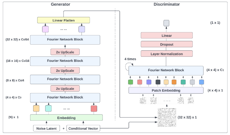
Structure of FCT-GAN. (Zhao et al., 2022)

Figure 1. Structure of FCT-GAN. (Zhao et al., 2022)

FCT-GAN excels in capturing intricate, nonlinear interactions that traditional GANs often miss, making it particularly effective for datasets with complex feature dependencies. However, it requires careful tuning of hyperparameters, such as the number of Fourier components, to balance the accuracy and computational complexity.

Tabular Denoising Diffusion Probabilistic Models (TabDDPM) (Kotelnikov et al., 2023) iteratively denoise a data distribution, capturing intricate dependencies by modeling the data generation process as a stochastic transformation. TabDDPM employs a combination of Gaussian diffusion for numerical features and multinomial diffusion for categorical and binary features, allowing it to handle mixed data types effectively. For a tabular data sample

$$\mathbf{x=[x_{\text{num}},x_{\text{cat}_{1}},\dots,x_{\text{cat}_{C}}]},$$

where $\mathbf{x_{\text{num}}}\in\mathbb{R}^{N_{\text{num}}}$ represents numerical features and $\mathbf{x_{\text{cat}_{i}}}$ represents categorical features with $K_{i}$ categories each, TabDDPM processes one-hot encoded categorical features and normalized numerical features. The model uses a multi-layer neural network to predict the noise $\epsilon$ for Gaussian diffusion and the categorical probabilities for multinomial diffusion during the reverse process. This enables TabDDPM to capture subtle correlations, such as how “debt-to-income ratio” and “employment history” jointly influence the “loan default” variable. For instance, a person with a high debt-to-income ratio and unstable employment history is more likely to default, a nuanced dependency preserved by the model. However, TabDDPM is computationally intensive, requiring a large number of iterations to achieve convergence. The model’s training involves minimizing a combined loss function

$$L^{\text{TabDDPM}}_{t}=L^{\text{simple}}_{t}+\frac{\sum_{i\leq C}L^{i}_{t}}{C},$$

where $L^{\text{simple}}_{t}$ is the mean-squared error for Gaussian diffusion (Eq.(13)), $L^{i}_{t}$ is the KL divergence for each multinomial diffusion term and $C$ represents the number of components or subsets over which the loss terms $L^{i}_{t}$ are averaged. This could correspond to different feature groups, categories, or partitions of the data in a tabular diffusion model. Additionally, hyperparameters such as the neural network architecture, time embeddings, and learning rates significantly influence the model’s effectiveness, making careful tuning essential for optimal performance.

The core strength of TabTransformer (Huang et al., 2020), lies in its ability to capture feature dependencies through its use of Transformer-based architectures (Vaswani et al., 2017). It leverages contextual embeddings to model the complex interactions between features, even in cases where those dependencies evolve over time or are not immediately apparent. The model achieves this by using the self-attention mechanism, which helps it to focus on the most relevant features for each record, taking into account both direct and indirect relationships. The self-attention mechanism calculates the dependencies between features using Eq. (14). This enables the model to learn and maintain dependencies between features even when their relationships are non-linear or complex. For instance, in a financial dataset, TabTransformer can capture the way features like payment history, loan amounts, and credit scores influence one another over time, maintaining these inter-feature dependencies across the entire dataset. This ability to focus on important features while preserving their interdependencies makes TabTransformer a powerful tool for generating synthetic tabular data that respects the underlying structure of the original data.

The structure of Tabular Masked Transformer (TabMT) (Gulati and Roysdon, 2023) is particularly well-suited for generating tabular data due to several key advantages, all of which contribute to its ability to maintain intricate feature dependencies. First, TabMT accounts for patterns bidirectionally between features. Unlike sequential data, tabular data lacks a natural ordering, meaning bidirectional learning enables the model to better understand and embed relationships between features, ensuring that dependencies between features are preserved. Second, TabMT’s masking procedure allows for arbitrary prompts during generation, making it uniquely flexible compared to other generators with limited conditioning capabilities. This flexibility ensures that the model can generate data while maintaining the relational structure of the original dataset, even when prompted with partial or non-sequential inputs. Third, TabMT handles missing data effectively by setting the masking probability for missing values to 1, whereas other generators often require separate imputation steps. This approach allows TabMT to learn and preserve dependencies even in the presence of incomplete data, ensuring high-quality synthetic samples.

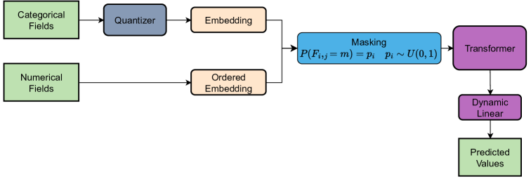
Figure 2. Diagram of TabMT. $m$ is the mask token, and $p_{i}$ is the masking probability of the $i$-th row. (Gulati and Roysdon, 2023)

Diagram of TabMT. $m$ is the mask token, and $p_{i}$ is the masking probability of the $i$-th row. (Gulati and Roysdon, 2023)

These structural advantages stem from TabMT’s novel masked generation procedure, which builds on the original BERT (Devlin, 2018) masking approach but introduces key modifications to improve generative performance. As illustrated in Figure 2, TabMT processes categorical and numerical fields separately. For categorical fields, a standard embedding matrix is used, while numerical fields are quantized and represented using ordered embeddings. The masking probability $p_{i}$ for the $i$-th row is sampled from a uniform distribution $U(0,1)$, ensuring that the training distribution of masked set sizes $|F^{m}_{i}|$ matches the uniform distribution encountered during generation. This is achieved by:

$$P(|F^{m}_{i}|=k)=\int_{0}^{1}\binom{l}{k}p^{k}(1-p)^{l-k}\,dp=\frac{1}{l+1}.$$

Additionally, TabMT predicts masked values in a random order during generation, addressing the mismatch between training and inference caused by fixed-order generation. This ensures that the model encounters each subset size uniformly, as:

$$P(F^{m}_{i}=s)=\frac{t!\cdot(l-t)!}{l!}=\frac{1}{\binom{l}{t}},$$

where $t$ is the generation step. These modifications, combined with the transformer architecture and dynamic linear layer, enable TabMT to generate high-quality synthetic data that preserves the relational structure and dependencies of the original dataset, even in the presence of missing values or heterogeneous data types.

Success and Limitations

The discussed models demonstrate varying strengths and limitations in preserving feature dependency for synthetic data generation. CTGAN effectively handles imbalanced data and captures simple feature dependencies but struggles with complex multi-way relationships (Zhao et al., 2021). CTAB-GAN balances the handling of mixed data types and captures both linear and non-linear interactions. However, due to its complex architecture, especially when learning dependencies across diverse data types and feature interactions, it can require significant computational resources. This is particularly true during the training phase, where the conditional GAN structure and the need for hyperparameter tuning can lead to increased training time and resource consumption. Additionally, the use of CNNs combined with one-hot encoding makes CTAB-GAN more vulnerable to column permutations, which can affect its robustness and generalizability in scenarios where the order of features varies (Zhao et al., 2022). FCT-GAN excels in modeling non-linear dependencies through Fourier transformations, though it requires careful hyperparameter tuning to achieve optimal performance (Zhao et al., 2022). Additionally, the use of Fourier transformations introduces significant computational complexity, making the model resource-intensive and less scalable for large datasets (Li et al., 2020). TabDDPM is highly effective at preserving intricate and subtle dependencies, as demonstrated by its ability to model complex data distributions through iterative denoising (Ho et al., 2020). However, this comes at the cost of being resource-intensive, requiring significant computational power for both training and sampling (Dhariwal and Nichol, 2021). Additionally, TabDDPM demands a large number of iterations to converge, which can lead to longer training times compared to other generative models (Nichol and Dhariwal, 2021). Lastly, Transformer-based models TabTransformer, TabMT are well-suited for temporal or sequential dependencies, leveraging their self-attention mechanisms to capture complex patterns in such data. However, they have limited utility for datasets lacking these structures, as their design is optimized for relational and sequential tasks (Vaswani et al., 2017). Each model addresses specific challenges, making their selection dependent on the dataset characteristics and application requirements.

3.2. Preserving Statistical Properties

Significance and Challenges

Preserving statistical properties such as distributions, correlations, and higher-order moments is essential for generating realistic synthetic data. In datasets like Credit Risk, maintaining these properties ensures that key insights, such as default rates and income distributions, remain valid for downstream applications like risk modeling and financial analysis (Figueira and Vaz, 2022). Distributions define the overall spread of data values, such as how annual incomes are distributed across different income brackets. If a real dataset shows that most individuals earn between $40,000 and $80,000, synthetic data should preserve this trend rather than generating incomes uniformly across all possible values. Correlations capture relationships between different features, such as how loan amounts typically increase with income. Ignoring these relationships in synthetic data may lead to misleading conclusions in financial modeling (Xu et al., 2019). Higher-order moments, such as skewness and kurtosis, further describe the shape of data distributions (Hoogeboom et al., 2021b). For instance, if loan defaults are heavily skewed toward lower-income groups, synthetic data should replicate this pattern to ensure accurate risk assessment.

One major challenge in preserving statistical properties is marginal distribution mismatch, where synthetic data fails to replicate the real distribution of individual features, such as “annual income” or “credit score,” leading to unrealistic results. A distorted income distribution, for example, could misrepresent credit risk levels (Patki et al., 2016). Another challenge is joint distribution representation, where capturing complex correlations between features, such as “loan amount” and “income,” becomes difficult as dimensionality increases (Nelsen, 2006). Additionally, rare event simulation poses difficulties, as rare but critical occurrences, like loan defaults, must be accurately reproduced for effective risk modeling(Figueira and Vaz, 2022).

Table 2. Preserving Statistical Properties Challenges and Models that address

Challenges	CTAB-GAN	Copula Flows	PrivBayes	STaSy	TABSYN	medGAN
Marginal Distribution Mismatch	✓		✓	✓	✓
Joint Distribution Representation	✓	✓		✓	✓	✓
Rare Event Simulation		✓		✓

Approaches

Several models have been developed to address the challenges of preserving statistical properties, particularly the distributional characteristics, correlations, and higher-order moments, in synthetic data generation. Each model offers unique methods for tackling these challenges, making them suitable for different types of data and application contexts. Table 2 summarizes how these models address specific challenges related to preserving statistical properties, highlighting their strengths and limitations.

CTAB-GAN preserves statistical properties through its Information Loss ($L^{G}_{\text{info}}$) Eq.(3), which ensures that the synthetic data matches the first-order (mean) and second-order (standard deviation) statistics of the real data. This loss is critical for maintaining the statistical integrity of the generated data. In addition, CTAB-GAN employs a variational Gaussian mixture model (VGM) (Bishop and Nasrabadi, 2006) to encode continuous features (e.g., credit scores, loan amounts) and one-hot encoding for categorical features (e.g., loan purpose, employment status). The VGM fits a mixture of Gaussian distributions to the data, ensuring accurate modeling of continuous feature distributions. However, the preservation of statistical properties is primarily enforced through the Information Loss, which explicitly matches the mean and variance of real and synthetic data. For example, in a credit risk dataset, CTAB-GAN uses $L^{G}_{\text{info}}$ to ensure that the synthetic data preserves the mean and variance of features such as credit scores and loan amounts. This is crucial for maintaining the statistical fidelity of the dataset, as it ensures that the synthetic data reflects the same central tendency and variability as the real data. However, CTAB-GAN may struggle with rare event simulation, such as generating high-risk borrowers with extremely low credit scores, due to the GAN’s tendency to underrepresent minority classes.

Copula Flows (Kamthe et al., 2021) preserve statistical properties by decomposing the joint distribution of the data into marginal distributions and a copula function. The joint density $f_{X}$ is expressed as:

$$f_{X}(X)=c_{X}(F_{X_{1}},\dots,F_{X_{d}})\prod_{k=1}^{d}f_{X_{k}}(X_{k}),$$

where $c_{X}$ is the copula density, $F_{X_{k}}$ are the marginal cumulative distribution functions (CDFs), and $f_{X_{k}}$ are the marginal densities. The marginal flows $F_{X_{k}}$ are trained using neural spline flows (Durkan et al., 2019) to approximate the true CDFs, ensuring that the synthetic data matches the marginal distributions of the original data. For example, in a credit risk dataset, the marginal flow for “credit scores” ensures that the synthetic credit scores have the same distribution as the real data, while the marginal flow for “loan amounts” preserves the distribution of loan values. The copula function $c_{X}$ captures the dependencies between features, preserving the joint distribution. For instance, in a credit risk dataset, the copula function ensures that the relationship between “credit scores” and “default rates” is maintained in the synthetic data. This is achieved by modeling the joint CDF $C_{X}(F_{X_{1}},\dots,F_{X_{d}})$, which describes how the marginal distributions interact. Copula Flows are particularly effective at capturing rare events, as they model tail dependencies in the data. However, their performance in rare event simulation can be affected by the representation of such events in the training data; if the rare events are too sparse or underrepresented, the model may struggle to generate them accurately.

Privacy-Preserving Bayesian Network (PrivBayes) (Zhang et al., 2017) preserves statistical properties by modeling the joint distribution of the data using a Bayesian network, which decomposes the joint distribution into a product of conditional distributions, as shown in Eq.( 15). PrivBayes learns the structure of the Bayesian network and the conditional distributions from the data, ensuring that the synthetic data matches the marginal and conditional distributions of the original data. By doing so, PrivBayes helps mitigate Marginal Distribution Mismatch, ensuring that the generated data accurately reflects the statistical properties of the original dataset at the feature level. For example, in a credit risk dataset, PrivBayes can model the conditional distribution of “default rates” given “credit scores” and “income levels”, ensuring that the synthetic data preserves these relationships. However, while it captures local dependencies, PrivBayes may not fully represent complex joint distributions across multiple features, limiting its ability to address joint distribution representation comprehensively. However, PrivBayes may struggle with rare event simulation, such as generating high-risk borrowers with extremely low credit scores, due to the limitations of Bayesian networks in capturing rare occurrences in the data.

Score-based Tabular Data Synthesis (STaSy) (Kim et al., 2022) is a model designed to preserve the statistical properties of tabular data by leveraging score-based generative models (Song et al., 2020b). Unlike traditional generative models, STaSy incorporates self-paced learning to ensure training stability. This allows for the generation of synthetic tabular data that accurately reflects the statistical properties of the original dataset. One key aspect of STaSy is its ability to preserve both the marginal distributions and the dependencies between features. The model iteratively refines noisy data by utilizing a denoising score matching objective, which approximates the gradient of the log-likelihood to ensure that the generated data aligns with the original data’s statistical characteristics.

The denoising score matching objective for the $i$-th record $x_{i}$ is defined by a function that measures the discrepancy between the predicted score and the gradient of the log-likelihood of the data. The denoising score matching loss for the $i$-th record is defined as follows:

$$l_{i}=\mathbb{E}_{t}\mathbb{E}_{\mathbf{x}_{i}(t)}\left[\lambda(t)\left\|S_{\theta}(\mathbf{x}_{i}(t),t)-\nabla_{\mathbf{x}_{i}(t)}\log p(\mathbf{x}_{i}(t)\mid\mathbf{x}_{i}(0))\right\|^{2}\right],$$

where $S_{\theta}(\mathbf{x}_{i}(t),t)$ is the score function, which estimates the gradient of the log-likelihood of the noisy data $\mathbf{x}_{i}(t)$, and $\lambda(t)$ is a scaling function that adjusts the emphasis on different noise scales during training. The function $\nabla_{\mathbf{x}_{i}(t)}\log p(\mathbf{x}_{i}(t)\mid\mathbf{x}_{i}(0))$ represents the true gradient of the log-likelihood, and $t$ refers to the noise level applied to the data. The STaSy objective function combines this score matching loss with a self-paced regularizer to effectively balance the model’s learning process, adjusting the contribution of each record during training. The overall objective is:

$$\min_{\theta,v}\sum_{i=1}^{N}v_{i}l_{i}+r(v;\alpha,\beta),$$

where $0\leq v_{i}\leq 1$ for all $i$, and $r(v;\alpha,\beta)$ is the self-paced regularizer. The parameters $\alpha$ and $\beta$, which belong to the interval $[0,1]$, control the thresholds for engagement in the training process as it progresses. The variable $v_{i}$ controls the participation of the $i$-th record, with a value of 1 indicating full participation and 0 indicating no participation.

STaSy addresses several key challenges in tabular data synthesis, including marginal distribution mismatch, joint distribution representation, and rare event simulation. First, to preserve the marginal distributions, STaSy uses its denoising process to ensure that the marginal distributions of each feature in the synthetic data closely match those of the original dataset. This is particularly important when dealing with features that follow complex or non-standard distributions. Second, STaSy ensures the preservation of joint distributions by modeling the dependencies between features through its score function. For example, in a credit risk dataset, STaSy can capture the relationships between features such as credit scores and loan amounts, ensuring that the joint distribution of these features is maintained in the synthetic data. Finally, STaSy effectively handles rare event simulation, which is often challenging in tabular data generation. By focusing on the tail regions of the distribution, STaSy can generate rare but significant data points, such as high-risk borrowers with low credit scores, ensuring that these rare events are accurately represented in the synthetic data. STaSy addresses this challenge by focusing on the tail regions of the distribution, ensuring that these rare yet significant events are represented in the synthetic data. This is particularly beneficial for training models on rare, high-impact cases, such as fraud detection or risk mitigation.

TABSYN (Zhang et al., 2023), a principled approach for tabular data synthesis preserves statistical properties through a two-stage process, as illustrated in Figure 3. In the first stage, each row of tabular data $\mathbf{x}=[\mathbf{x}^{\text{num}},\mathbf{x}^{\text{cat}}]$ is mapped to a latent space $z$ using a column-wise tokenizer and an encoder. The tokenizer converts each column (both numerical and categorical) into a $d$-dimensional vector. For numerical columns, the tokenizer applies a linear transformation:

$$e^{\text{num}}_{i}=\mathbf{x}^{\text{num}}_{i}\cdot w^{\text{num}}_{i}+b^{\text{num}}_{i},$$

where $w^{\text{num}}_{i}$ and $b^{\text{num}}_{i}$ are learnable parameters. For categorical columns, the tokenizer uses an embedding lookup:

$$e^{\text{cat}}_{i}=\mathbf{x}^{\text{oh}}_{i}\cdot W^{\text{cat}}_{i}+b^{\text{cat}}_{i},$$

where $\mathbf{x}^{\text{oh}}_{i}$ is the one-hot encoded categorical feature, and $W^{\text{cat}}_{i}$ and $b^{\text{cat}}_{i}$ are learnable parameters. The tokenized representations $E=[e^{\text{num}}_{1},\dots,e^{\text{num}}_{M_{\text{num}}},e^{\text{cat}}_{1},\dots,e^{\text{cat}}_{M_{\text{cat}}}]$ are fed into a Transformer-based encoder to produce latent embeddings $z$. This ensures that the synthetic data retains the marginal distributions of individual features, such as credit scores and loan amounts in a creditrisk dataset.

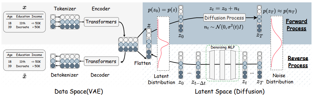
An overview of the proposed TABSYN. Each row of tabular data $\mathbf{x}$ is mapped to a latent space $z$ via a column-wise tokenizer and an encoder. A diffusion process $z_{0}\rightarrow z_{T}$ is applied in the latent space. Synthesis $z_{T}\rightarrow z_{0}$ starts from the base distribution $p(z_{T})$ and generates samples $z_{0}$ in the latent space through a reverse process. These samples are then mapped from the latent space $z$ to the data space $\tilde{x}$ using a decoder and a detokenizer (Zhang et al., 2023).

Figure 3. An overview of the proposed TABSYN. Each row of tabular data $\mathbf{x}$ is mapped to a latent space $z$ via a column-wise tokenizer and an encoder. A diffusion process $z_{0}\rightarrow z_{T}$ is applied in the latent space. Synthesis $z_{T}\rightarrow z_{0}$ starts from the base distribution $p(z_{T})$ and generates samples $z_{0}$ in the latent space through a reverse process. These samples are then mapped from the latent space $z$ to the data space $\tilde{x}$ using a decoder and a detokenizer (Zhang et al., 2023).

In the second stage, a diffusion process is applied in the latent space. The forward process gradually adds noise to the latent embeddings $z_{0}\rightarrow z_{T}$:

$$z_{t}=z_{0}+\sigma(t)\epsilon,\quad\epsilon\sim\mathcal{N}(0,I),$$

where $\sigma(t)$ is the noise level at time $t$. The reverse process denoises the embeddings $z_{T}\rightarrow z_{0}$, starting from a base distribution $p(z_{T})$. This ensures that the synthetic data preserves the joint distribution of features, such as the relationship between credit scores and default rates. Finally, the latent embeddings $z_{0}$ are mapped back to the data space $\tilde{x}$ using a decoder and detokenizer:

$$\tilde{\mathbf{x}}^{\text{num}}_{i}=\tilde{e}^{\text{num}}_{i}\cdot\tilde{w}^{\text{num}}_{i}+\tilde{b}^{\text{num}}_{i},\quad\tilde{\mathbf{x}}^{\text{cat}}_{i}=\text{Softmax}(\tilde{e}^{\text{cat}}_{i}\cdot\tilde{W}^{\text{cat}}_{i}+\tilde{b}^{\text{cat}}_{i}),$$

where $\tilde{w}^{\text{num}}_{i}$, $\tilde{b}^{\text{num}}_{i}$, $\tilde{W}^{\text{cat}}_{i}$, and $\tilde{b}^{\text{cat}}_{i}$ are learnable parameters of the detokenizer.

TABSYN effectively addresses marginal distribution mismatch and joint distribution representation by leveraging the tokenizer and encoder to model marginal distributions and the diffusion process to capture dependencies between features. However, it may struggle with Rare Event Simulation, such as generating high-risk borrowers with extremely low credit scores, due to the diffusion process’s focus on the bulk of the data distribution rather than the tails.

Medical Generative Adversarial Network (medGAN) (Choi et al., 2017) preserves the statistical properties of the original electronic health records (EHR) data through a combination of an autoencoder and generative adversarial networks (GANs). The autoencoder, comprising an encoder Enc and a decoder Dec, is pre-trained to learn the salient features of the input data $\mathbf{x}\in\mathbb{Z}_{+}^{|C|}$. The encoder compresses $\mathbf{x}$ into a latent representation $\text{Enc}(\mathbf{x})\in\mathbb{R}^{h}$, and the decoder reconstructs it, minimizing the reconstruction loss, $L_{R}$:

$$L_{R}=\begin{cases}\large\frac{1}{m}\sum_{i=0}^{m}\|\mathbf{x}_{i}-\mathbf{x}^{\prime}_{i}\|_{2}^{2}&\quad\text{if }\mathbf{x}_{i}\text{ is a count variable}\\ \vskip-8.5359pt\\ \frac{1}{m}\sum_{i=0}^{m}\mathbf{x}_{i}\log\mathbf{x}^{\prime}_{i}+(1-\mathbf{x}_{i})\log(1-\mathbf{x}^{\prime}_{i})&\quad\text{if }\mathbf{x}_{i}\text{ is a binary variable}\end{cases}$$

where $\mathbf{x}^{\prime}_{i}=\text{Dec}(\text{Enc}(\mathbf{x}_{i}))$. As shown in the architecture diagram (Figure  4), the generator $G$ takes a random prior $\mathbf{z}\in\mathbb{R}^{r}$ and produces synthetic data $G(\mathbf{z})$, which is then mapped to discrete values using the pre-trained decoder $\text{Dec}(G(\mathbf{z}))$. The discriminator $D$ is trained to distinguish between real data $\mathbf{x}$ and synthetic data $\text{Dec}(G(\mathbf{z}))$, ensuring that the synthetic data matches the distribution of the real data through the adversarial objective:

$$\min_{G}\max_{D}V(G,D)=\mathbb{E}_{\mathbf{x}\sim p_{\text{data}}}[\log D(\mathbf{x})]+\mathbb{E}_{\mathbf{z}\sim p_{z}}[\log(1-D(\text{Dec}(G(\mathbf{z}))))].$$

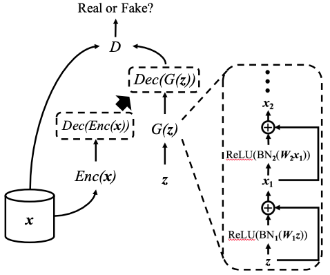
Architecture of medGAN: The discrete $\mathbf{x}$ comes from the source EHR data, $\mathbf{z}$ is the random prior for the generator $G$; $G$ is a feedforward network with shortcut connections (right-hand side figure); An autoencoder (i.e., the encoder Enc and decoder Dec) is learned from $\mathbf{x}$; The same decoder Dec is used after the generator $G$ to construct the discrete output. The discriminator $D$ tries to differentiate real input $\mathbf{x}$ and discrete synthetic output $\text{Dec}(G(\mathbf{z}))$ (Choi et al., 2017).

Figure 4. Architecture of medGAN: The discrete $\mathbf{x}$ comes from the source EHR data, $\mathbf{z}$ is the random prior for the generator $G$; $G$ is a feedforward network with shortcut connections (right-hand side figure); An autoencoder (i.e., the encoder Enc and decoder Dec) is learned from $\mathbf{x}$; The same decoder Dec is used after the generator $G$ to construct the discrete output. The discriminator $D$ tries to differentiate real input $\mathbf{x}$ and discrete synthetic output $\text{Dec}(G(\mathbf{z}))$ (Choi et al., 2017).

To prevent mode collapse, medGAN introduces minibatch averaging, where the discriminator is provided with the average of minibatch samples:

$$\theta_{d}\leftarrow\theta_{d}+\alpha\nabla_{\theta_{d}}\frac{1}{m}\sum_{i=1}^{m}\log D(\mathbf{x}_{i},\bar{\mathbf{x}})+\log(1-D(\mathbf{x}_{z_{i}},\bar{\mathbf{x}}_{z})),$$

where $\bar{\mathbf{x}}=\frac{1}{m}\sum_{i=1}^{m}\mathbf{x}_{i}$ and $\bar{\mathbf{x}}_{z}=\frac{1}{m}\sum_{i=1}^{m}\mathbf{x}_{z_{i}}$. Additionally, batch normalization and shortcut connections are used to stabilize training and improve learning efficiency. Despite these strengths, medGAN has limitations. It does not explicitly address feature dependencies, which could lead to unrealistic relationships between variables in the generated data. The model also lacks mechanisms for conditioning on specific attributes, limiting its ability to generate targeted synthetic data for specific subsets of patients. Furthermore, while minibatch averaging helps prevent mode collapse, the model may still struggle with highly imbalanced datasets or rare categories. Finally, the reliance on GANs makes training computationally expensive and sensitive to hyperparameter tuning, which could hinder scalability and practicality in real-world applications.

Success and Limitations

Preserving statistical properties in synthetic data generation has yielded significant progress, enhancing data utility and enabling robust applications across various domains. A key success lies in ensuring synthetic datasets mirror the statistical characteristics of real data, making them viable for downstream tasks like model training, fairness evaluation, and bias mitigation. Additionally, these techniques have empowered scenario analysis and stress testing, particularly in high-stakes domains where understanding rare events and tail risks is critical. By capturing complex feature dependencies, models that prioritize statistical fidelity improve the reliability of synthetic data for predictive analytics and decision-making.

However, preserving statistical properties introduces several challenges. Ensuring accurate reproduction of both marginal and joint distributions is non-trivial, especially with heterogeneous data types and intricate feature relationships. One notable limitation is the risk of overfitting, where synthetic data closely mimics the original, inadvertently compromising privacy. Moreover, balancing privacy and utility poses a constant trade-off, models that focus on statistical accuracy may reveal subtle patterns that adversaries could exploit. Another persistent challenge is generalizability: techniques optimized for one domain may struggle to adapt to others due to differing data structures and contextual dependencies. Computational complexity is also a concern, as capturing nuanced statistical relationships demands more sophisticated architectures and prolonged training times, limiting scalability. These successes and limitations reflect the ongoing effort to balance statistical fidelity, privacy preservation, and computational efficiency in synthetic data generation.

3.3. Preserving Data Privacy

Significance and Challenges

Privacy preservation is essential in synthetic data generation, particularly for sensitive datasets such as Credit Risk, which contain personal financial details (Dwork et al., 2014). The challenge lies in ensuring that synthetic data maintains statistical utility for tasks like credit risk assessment while preventing adversaries from inferring sensitive attributes. Synthetic data should protect individuals’ information while preserving patterns that make it useful for downstream tasks. Techniques such as differential privacy have emerged as a key solution, as highlighted in foundational works like (Dwork et al., 2014). One of the primary risks is reconstruction attacks, where adversaries attempt to reverse-engineer real data from synthetic datasets. If synthetic records closely resemble actual individuals’ data, attackers can infer attributes such as income, loan amount, or credit score. A notable form of reconstruction attack is the model inversion attack (Fredrikson et al., 2014), where an attacker exploits a trained model to infer missing attributes. For example, if a credit approval model is trained on features such as age, employment status, and credit score, an attacker with partial knowledge of an applicant’s details can repeatedly query the model to uncover sensitive information. Another vulnerability arises from attribute inference attacks, where statistical correlations in synthetic data reveal sensitive relationships. If synthetic data preserves a strong link between high-income individuals and loan approvals, an attacker could deduce an applicant’s financial status with high probability. Preventing such attacks requires techniques that prevent direct memorization, introduce privacy constraints, and reduce overfitting to real data. These risks are extensively discussed in (Yeom et al., 2018). Another major challenge is balancing the privacy-utility trade-off. Methods such as differential privacy inject noise into data or model training to obscure individual records, but excessive noise can distort statistical relationships, making the synthetic data less useful. Conversely, prioritizing utility without sufficient privacy safeguards increases vulnerability to attacks. A well-designed synthetic data model must ensure that data remains useful while mitigating privacy risks, particularly in regulated sectors like finance, where data breaches have legal and ethical implications. The trade-offs between privacy and utility are explored in (Bindschaedler et al., 2017).

Table 3. Privacy-preserving approaches address the following key challenges in synthetic data generation

Challenges	DP-SYN	PATE-GAN	PrivBayes	DP-CTGAN	IT-GAN	EHR-Safe
Prevents Direct Memorization	✓	✓	✓	✓	✓
Protects Against
Model Inversion Attacks	✓	✓	✓
Handles Attribute
Inference Risks	✓	✓	✓			✓
Preserves Feature
Dependencies		✓	✓	✓	✓	✓

Approaches

Several privacy-preserving synthetic data generation models have been developed to address these challenges. Table 3 summarizes how different privacy-preserving synthetic data generation models handle common challenges, such as preventing direct memorization, protecting against model inversion attacks, and preserving feature dependencies.

Differentially private synthetic data generation (DP-SYN) (Abay et al., 2019) preserves privacy by combining a differentially private auto-encoder (DP-Auto) with a differentially private expectation maximization (DP-EM) algorithm. As shown in Figure 5, the process begins by partitioning the credit risk data set $D$ into $k$ groups based on labels (e.g., “Credit Risk” and “Non-Credit Risk”). The privacy budget $\epsilon$ and $\delta$ are then allocated across these groups, ensuring that privacy is maintained within each subset. The allocation is proportional to the size of each group, so larger groups receive a slightly higher budget.

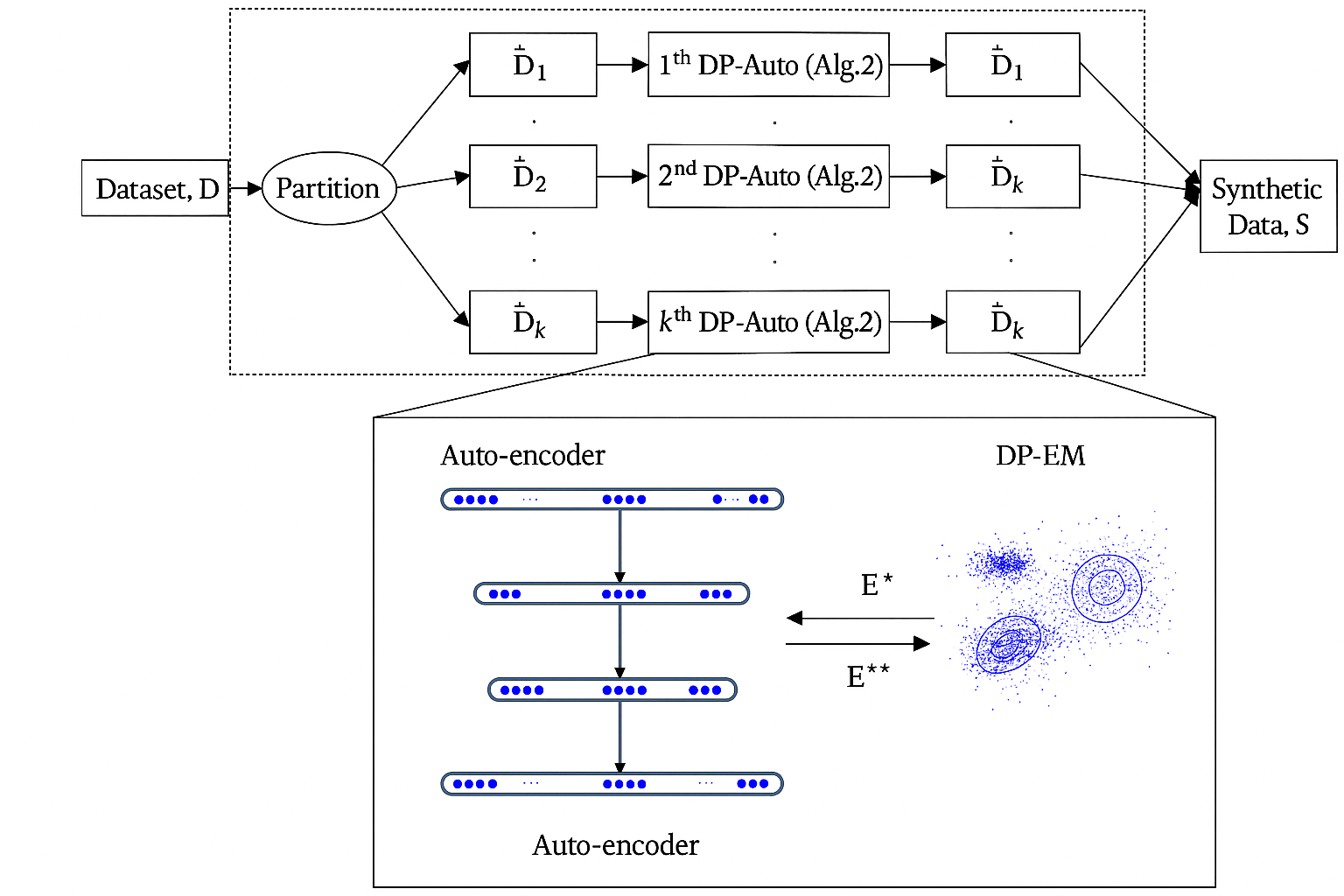
Differentially private synthetic data generation

Figure 5. Differentially private synthetic data generation $DP-SYN$ (Abay et al., 2019).

Next, a private auto-encoder is trained for each group. During training, Gaussian noise $z_{it}\sim N(0,\sigma^{2}C^{2})$ is added to the gradients of the model to ensure differential privacy. For example, in the case of the Credit Risk dataset, features such as ‘income‘, ‘age‘, and ‘loan amount‘ are encoded into a latent representation, preserving their general patterns but obscuring any individual data points. The model parameters $w_{t}$ are updated with this noisy gradient, which helps prevent the model from memorizing sensitive information about individuals. The update rule for the model is:

$$w_{t+1}=w_{t}-\eta\cdot\left(\frac{1}{|B_{t}|}\sum_{i_{t}}\left(\nabla\ell(w_{t};\mathbf{x}_{it})+z_{it}\right)\right),$$

where $\eta$ is the learning rate and $|B_{t}|$ is the batch size. This process is repeated until the model converges or the privacy budget $\epsilon_{A}$ is exhausted.

The encoded data is then processed by the DP-EM algorithm, which identifies latent patterns and generates synthetic data with statistical properties similar to the original dataset. For example, the DP-EM algorithm synthesizes data that reflects the distribution of features like “loan amount” and “credit score”, ensuring that feature dependencies are preserved without revealing individual data. This step is critical to maintaining the relationships between different attributes while preventing the inference of private information. Finally, the synthetic data is decoded and aggregated to form a complete synthetic dataset, as shown in Figure 5. Throughout this process, privacy is guaranteed by tracking the cumulative privacy loss using the moments accountant method, ensuring that the overall privacy budget is not exceeded. The result is a synthetic dataset that maintains the statistical properties of the original data while providing privacy guarantees.

Private Aggregation of Teacher Ensembles GAN (PATE-GAN) (Jordon et al., 2018) preserves privacy by incorporating the PATE mechanism into the GAN framework, ensuring differential privacy during training. In the standard GAN framework, the generator $G$ is trained to minimize its loss with respect to a discriminator $D$, using loss function Eq.(11) where $G(z)$ is the generated sample and $D$ is the discriminator that tries to distinguish between real and fake data. In PATE-GAN, the discriminator is replaced by a student discriminator, $S$, which is trained using noisy labels generated by teacher-discriminators $T_{1},T_{2},\dots,T_{k}$. The teacher-discriminators are trained on disjoint subsets of the data, with their empirical loss defined as:

$$L_{i}^{T}(\theta_{i}^{T})=-\left(\sum_{u\in D_{i}}\log T_{i}(u;\theta_{i}^{T})+\sum_{j=1}^{n}\log(1-T_{i}(G(z_{j});\theta_{i}^{T}))\right),$$

where $D_{i}$ is the partitioned dataset for teacher $T_{i}$, and each teacher classifies real and fake samples independently. The student-discriminator $S$ is trained using the noisy labels from the teachers. The loss function for the student-discriminator is:

$$L_{S}(\theta_{S})=\sum_{j=1}^{n}r_{j}\log S(u_{j};\theta_{S})+(1-r_{j})\log(1-S(u_{j};\theta_{S})),$$

where $r_{j}$ are the noisy labels assigned by the teachers through the PATE mechanism. Finally, the generator $G$ is trained to minimize the loss with respect to the student-discriminator:

$$L_{G}(\theta_{G};S)=\sum_{j=1}^{n}\log(1-S(G(z_{j};\theta_{G}))).$$

This loss is similar to the original GAN generator loss Eq.(12) , but the discriminator has been replaced by the student, which provides differential privacy guarantees. By training the student with noisy teacher labels and ensuring it is exposed only to generated samples, PATE-GAN effectively prevents direct memorization, protects against model inversion attacks, handles attribute inference risks, and preserves feature dependencies in the synthetic data. Differential privacy is ensured through the PATE mechanism, and the moments accountant method is used to calculate the privacy guarantee for the entire process.

Privacy-Preserving Bayesian Network (PrivBayes) (Zhang et al., 2017) is a synthetic data generation technique that leverages Bayesian networks to model feature dependencies while ensuring differential privacy. The method builds a Bayesian network to capture the joint distribution of features, where each node represents a feature and edges represent conditional dependencies between them. To preserve privacy, PrivBayes introduces Laplace noise to the parameters of the Bayesian network using the Laplace mechanism. The general loss function for the Bayesian network parameter estimation, including the Laplace noise, is expressed as:

$$L(\theta)=\sum_{i=1}^{n}\log P(\mathbf{x}_{i}|\theta)+\text{Laplace noise},$$

where $P(\mathbf{x}_{i}|\theta)$ is the conditional probability for feature set $x_{i}$ and $\theta$ are the parameters of the network. The Laplace noise is calibrated based on the sensitivity of queries made on the data and the privacy parameter $\epsilon$, ensuring differential privacy by adding noise that prevents direct memorization and reconstruction of individual data points. This approach mitigates risks such as model inversion attacks and attribute inference, as the noisy parameters make it difficult for attackers to accurately infer sensitive attributes. The method also preserves feature dependencies, generating synthetic data that mimics the statistical properties of the original data as discussed in Section 3.2. The differential privacy mechanism ensures privacy by calibrating the scale of the Laplace noise, which is inversely proportional to the sensitivity of the query and the privacy parameter $\epsilon$, maintaining a balance between privacy protection and data utility.

DP-CTGAN (Fang et al., 2022) integrates differential privacy (DP) into CTGAN to generate synthetic tabular data while ensuring privacy preservation (Figure 6). The model employs a privacy accountant to track privacy loss and incorporates differential privacy into the training process. The core privacy mechanism follows the Gaussian mechanism, where noise is added to the gradients of the critic (discriminator) rather than the generator to maintain convergence stability. Given a privacy budget $(\epsilon_{0},\delta_{0})$, the model ensures that the total privacy loss remains within acceptable bounds.

The loss function of the critic is defined as:

(4) $$L_{C}=\frac{1}{s}\sum_{k=1}^{s}\left(C(\hat{r}_{j}^{k},\text{cond}_{j}^{k})-C(r_{j}^{k},\text{cond}_{j}^{k})\right)+L_{GP},$$

where $C(\cdot)$ represents the critic’s evaluation, $\hat{r}_{j}^{k}$ and $r_{j}^{k}$ denote synthetic and real samples conditioned on $\text{cond}_{j}^{k}$, and $L_{GP}$ is the gradient penalty term ensuring Lipschitz continuity. Differential privacy is enforced by adding Gaussian noise $\xi\sim\mathcal{N}(0,\sigma_{C}^{2}I)$ to the critic’s gradient updates:

(5) $$\Phi_{C}\leftarrow\Phi_{C}-0.0002\times\text{Adam}(\nabla_{\Phi_{C}}(L_{C}+10L_{GP}+\xi)).$$

The generator loss is defined as:

(6) $$L_{G}=\frac{1}{m}\sum_{j=1}^{m}\text{CrossEntropy}(\hat{d}_{i^{*},j},m_{i^{*}})-\frac{1}{m/s}\sum_{k=1}^{m/s}C(\hat{r}_{s}^{k},\text{cond}_{s}^{k}),$$

where the first term ensures accurate generation of categorical variables using cross-entropy loss, and the second term minimizes the critic’s ability to distinguish real and synthetic samples. The generator parameters are updated as:

(7) $$\Phi_{G}\leftarrow\Phi_{G}-0.0002\times\text{Adam}(\nabla_{\Phi_{G}}L_{G}).$$

To prevent direct memorization and model inversion attacks, DP-CTGAN ensures that only the critic interacts with real data, and the added noise limits adversaries from inferring individual data points. The privacy budget $(\epsilon,\delta)$ is updated iteratively:

(8) $$\epsilon\leftarrow\text{query }A\text{ with }\delta_{0},$$

where $A$ represents the privacy accountant tracking cumulative privacy loss. Feature dependencies are preserved through mode-specific normalization and conditional sampling, ensuring balanced data generation for categorical attributes. By integrating differential privacy and leveraging CTGAN’s ability to model complex tabular data distributions, DP-CTGAN effectively generates privacy-preserving synthetic data while mitigating attribute inference risks and maintaining statistical fidelity.

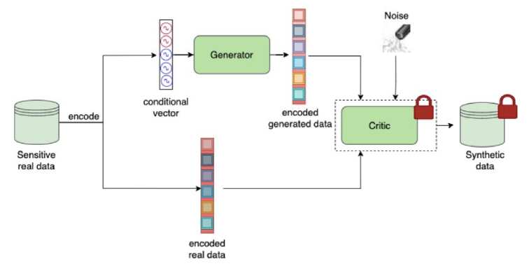
Figure 6. DP-CTGAN. Sensitive training data is fed into a conditional generator to generate samples which can evenly cover all possible discrete values. At the same time, random perturbation is added to the critic to enforce privacy protection (Fang et al., 2022).

CTGAN with differential privacy a potential approach for privacy-preserving synthetic data generation is adding differential privacy to the CTGAN framework. This technique helps mitigate privacy risks by ensuring that the synthetic data does not reveal private information about individuals. Although this approach offers some degree of privacy protection, its guarantees are not as robust as those provided by models like DP-SYN or PATE-GAN. Additionally, the introduced noise may hinder the model’s ability to learn complex data distributions. While this method has been demonstrated with medical data, it could be extended to other domains such as credit risk modeling to protect sensitive financial information.

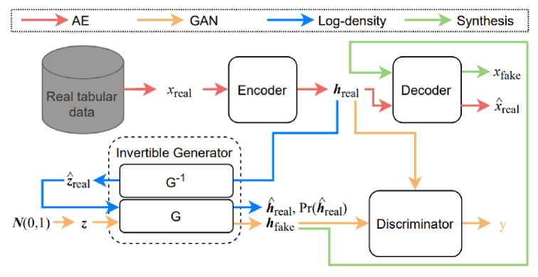
Figure 7. The overall architecture of IT-GAN. Each edge color means a certain type of data path (Lee et al., 2021).

The Invertible Tabular GAN (IT-GAN) (Lee et al., 2021) preserves privacy by integrating adversarial training from GANs with the log-density training of invertible neural networks, enabling a trade-off between synthesis quality and privacy protection. The architecture, depicted in Figure  7, consists of four key data paths: the AE-path, log-density-path, GAN-path, and synthesis-path. The AE-path uses an autoencoder (AE) to transform real records $\mathbf{x}_{\text{real}}$ into hidden representations $h_{\text{real}}$ and reconstructs them as $\hat{\mathbf{x}}_{\text{real}}$. The encoder $E$ and decoder $R$ are defined as:

$$h_{\text{real}}=E(\mathbf{x}_{\text{real}})=\text{FC}_{1n_{e}}(\dots\phi(\text{FC}_{11}(x_{\text{real}}))\dots),$$

$$\hat{\mathbf{x}}_{\text{real}}=R(h_{\text{real}})=\text{FC}_{2n_{r}}(\dots\phi(\text{FC}_{21}(h_{\text{real}}))\dots),$$

where $\phi$ is a ReLU activation, FC denotes fully connected layers, and $n_{e}$ and $n_{r}$ represent the number of layers in the encoder and decoder, respectively. The log-density-path leverages an invertible neural network to compute the log-density of $h_{\text{real}}$, denoted as $\log\hat{p}_{g}(h_{\text{real}})$, which approximates the log-density of the real data. This ensures that the generated data distribution aligns closely with the real data distribution, enhancing privacy. The generator $G$, based on Neural Ordinary Differential Equations (NODEs), is defined as:

$$h_{\text{fake}}=z(0)+\int_{0}^{1}f(z(t),t;\theta_{g})\,dt,$$

where $f(z,t;\theta_{g})$ is a learnable function, and $z(0)\sim\mathcal{N}(0,1)$ is a latent vector sampled from a unit Gaussian. The log-probability $\log p(h_{\text{fake}})$ is estimated using the Hutchinson estimator:

$$\log p(h_{\text{fake}})=\log p(z(0))-\mathbb{E}_{p(\epsilon)}\left[\int_{0}^{1}\epsilon^{\top}\frac{\partial f}{\partial z(t)}\epsilon\,dt\right].$$

The GAN-path employs adversarial training, where the discriminator $D$ distinguishes between $h_{\text{real}}$ and $h_{\text{fake}}$. The synthesis-path generates synthetic records post-training using the generator and decoder. Privacy is further reinforced by the AE’s mode-specific normalization, which discretizes continuous data into Gaussian mixtures and one-hot vectors, reducing the risk of re-identification. The training algorithm optimizes the model using a combination of reconstruction loss $L_{\text{AE}}$, WGAN-GP loss, and a log-density regularizer $R_{\text{density}}$, defined as:

$$L_{\text{AE}}=L_{\text{Reconstruct}}+\frac{1}{2}\|h_{\text{real}}\|^{2}+\|h_{\text{fake}}-\hat{h}_{\text{fake}}\|^{2},$$

$$R_{\text{density}}=\gamma\mathbb{E}_{x\sim p_{\text{data}}}\left[-\log\hat{p}(E(\mathbf{x}))\right],$$

where $\gamma$ controls the regularization strength. Despite its advancements, IT-GAN has several limitations that impact its practical application. First, the loss of fine-grained details during mode-specific normalization, while effective for preserving privacy, may compromise the synthesis quality for certain applications by discarding subtle but important information in the data. Second, the scalability of the model is constrained by the computational overhead introduced by the Hutchinson estimator, which, although unbiased, increases the complexity and resource requirements, making it less suitable for very large datasets. Finally, the training stability of IT-GAN is challenged by the integration of multiple loss functions, such as $L_{\text{AE}}$, WGAN-GP, and $R_{\text{density}}$, which can lead to instability and necessitate careful hyperparameter tuning to achieve optimal performance. These limitations highlight the trade-offs involved in balancing privacy preservation, synthesis quality, and computational efficiency in IT-GAN.

EHR-Safe (Yoon et al., 2023) is a privacy-preserving synthetic data generation model designed to generate synthetic electronic health records (EHR) while preserving the privacy of sensitive information. The methodology includes encoding and decoding features, normalizing complex distributions, conditioning adversarial training, and handling missing data. This is achieved through a deep encoder-decoder architecture, which is also adaptable to other datasets. For example, categorical features such as “loan status” or “employment type” are encoded into abstract representations, which do not directly expose sensitive information. The encoder-decoder mechanism is optimized to transform categorical features through the following loss function for static categorical data:

$$\mathop{\min}\limits_{C{E}^{s},C{F}_{1}^{s},...,C{F}_{K}^{s}}\mathop{\sum}\limits_{k=1}^{K}{{{{{L}}}}}_{c}(C{F}_{i}^{s}[CE[{s}_{1}^{co},...,{s}_{K}^{co}]],{s}_{i}^{co}),$$

where $C{E}^{s}$ is the encoder for the static categorical features, $C{F}_{k}^{s}$ is the decoder for each categorical feature, and ${s}_{co}$ represents the one-hot encoded categorical feature values (e.g., “loan status” encoded as 1 for “approved” or 0 for “denied” in credit risk data). For temporal categorical features (such as monthly payment status over time), the following loss function is used:

$$\mathop{\min}\limits_{C{E}^{t},C{F}_{1}^{t},...,C{F}_{K}^{t}}\mathop{\sum}\limits_{k=1}^{K}{{{{{L}}}}}_{c}(C{F}_{i}^{t}[CE[{t}_{1}^{co},...,{t}_{K}^{co}]],{t}_{i}^{co}),$$

where $C{E}^{t}$ and $C{F}_{k}^{t}$ correspond to the temporal categorical encoder and decoder, respectively, and ${t}_{co}$ represents the one-hot encoded temporal feature values. This model also uses stochastic normalization for numerical features, such as “annual income” and “loan amount” . This normalization step ensures that the distribution of numerical values is consistent and maintains privacy. The stochastic normalization function is defined as follows:

$$\mathbf{X}^{\text{normalized}}=\text{StochasticNormalization}(\mathbf{X}),$$

where $\mathbf{X}$ represents a numerical feature, such as “income” or “loan amount”. The stochastic normalization process adjusts the feature distribution while preserving the underlying statistical properties.

A key innovation of EHR-Safe is its use of adversarial training with a Wasserstein GAN with Gradient Penalty (WGAN-GP) to train the generator and discriminator. The objective of adversarial training is to generate synthetic data that is indistinguishable from real data. The adversarial loss function is:

$$\mathbf{\max}_{G}\mathbf{\min}_{D}\frac{1}{N}\sum_{i=1}^{N}D(e[i])-\frac{1}{N}\sum_{i=1}^{N}D(\hat{e}[i])+\eta\left(\left|\left|\nabla_{D}(\hat{e}[i])\right|\right|-1\right)^{2},$$

where $e[i]$ represents the real encoder state, $\hat{e}[i]$ is the synthetic encoder state generated by the model, and $\eta$ is the gradient penalty factor. The generator $G$ aims to create synthetic data that matches the real data distribution, while the discriminator $D$ tries to distinguish between real and synthetic data. In addition, EHR-Safe generates realistic missing patterns for missing data (e.g. missing “credit score” values). The missing patterns are represented as:

$$D_{M}=\{m_{n}(i),m_{c}(i),m_{\tau n}(i),m_{\tau c}(i)\}_{i=1}^{N},$$

where $m_{n}(i)$ and $m_{c}(i)$ represent missing patterns for numerical and categorical features, and $m_{\tau n}(i)$ and $m_{\tau c}(i)$ are the missing patterns for temporal features. These missing patterns help maintain the structural integrity of the synthetic data and avoid information leakage. Finally, in the inference phase, synthetic data is generated by sampling random vectors from a Gaussian distribution and passing them through the trained generator $G$. The synthetic encoder states $\hat{e}$ are then decoded to synthetic data, including categorical and numerical features and missing patterns. The final synthetic dataset is generated as follows:

$$\hat{e}=G(z),\quad\text{where }z\sim N(0,I),$$

$$(\hat{s}_{n},\hat{s}_{ce},\hat{t}_{n},\hat{t}_{ce},\hat{u},\hat{m}_{n},\hat{m}_{c},\hat{m}_{\tau n},\hat{m}_{\tau c})=F(\hat{e}).$$

The synthetic data includes features like “loan amount” ($\hat{s}_{n}$), “loan status” ($\hat{s}_{c}$), “monthly payment” ($\hat{t}_{n}$), and missing patterns, such as $\hat{m}_{n}$ for numerical features or $\hat{m}_{c}$ for categorical features. The final synthetic data output is:

$$\hat{D}=\{\hat{s}_{n}(i),\hat{s}_{c}(i),\hat{u},\hat{m}_{n}(i),\hat{m}_{c}(i),\hat{m}_{\tau n}(i),\hat{m}_{\tau c}(i)\}_{i=1}^{M},$$

where $M$ is the number of synthetic samples generated. This synthetic data is useful for tasks like credit scoring or risk assessment, while maintaining privacy and ensuring data utility. Through these mechanisms, EHR-Safe provides a robust solution for generating privacy-preserving synthetic data from different datasets, ensuring both the confidentiality of sensitive data and the utility of the generated data for analysis and modeling purposes. While the model is effective in generating privacy-preserving synthetic data, it assumes that feature distributions can be normalized to fully preserve privacy while maintaining data utility, which may not always hold true for datasets with complex dependencies or rare categorical values. Furthermore, the approach to missing data generation assumes a uniform missingness mechanism, which may not fully capture the complexities of real-world missing data patterns. Finally, the model may struggle to generate high-quality synthetic data in domains with highly heterogeneous features or extreme feature interactions, such as in healthcare or finance.

Success and Limitations

Privacy-preserving models have demonstrated their ability to mitigate risks such as model inversion and attribute inference attacks, making synthetic data safer for sharing and analysis. Techniques like differential privacy provide formal guarantees that limit the leakage of sensitive information, even when adversaries attempt to reverse-engineer the original data (Abay et al., 2019). Additionally, these models show promise in balancing privacy and utility by preserving key statistical properties and feature dependencies, enabling synthetic data to remain useful in downstream tasks like machine learning training and predictive modeling (Jordon et al., 2018). However, these models face notable challenges. The privacy-utility trade-off remains a persistent issue, stronger privacy guarantees often come at the expense of data fidelity, reducing the synthetic dataset’s usefulness. High-dimensional datasets such as credit risk (Kaggle, nd) and adult (Becker and Kohavi, 1996) datasets amplify this challenge, where achieving both privacy and utility becomes increasingly complex (Papernot et al., 2016). Scalability is another limitation, as models tailored to privacy preservation sometimes struggle with large datasets or require computationally expensive mechanisms, making them less practical for real-time applications (Yoon et al., 2023). Furthermore, the effectiveness of some privacy-preserving techniques is highly dependent on the quality and diversity of training data. Biased or imbalanced datasets can lead to privacy leaks and unstable synthetic data generation. Finally, many approaches lack robustness against evolving attack strategies (Guan et al., 2024; Annamalai et al., 2024), which increasingly enable inference of sensitive information from synthetic or aggregated data, highlighting the need for stronger privacy guarantees.

3.4. Conditioning on Specific Attributes

Significance and Challenges

Conditioning in synthetic data generation enables targeted sampling (Goodfellow et al., 2014), allowing models to generate specific subpopulations while preserving statistical properties. In Credit Risk, this is crucial for simulating borrower segments based on factors such as loan grade, interest rate, or annual income. Effective conditioning ensures that generated records remain realistic, meaning synthetic applicants conditioned on high-interest loans should exhibit higher default rates, consistent with real-world trends. This capability is essential for financial institutions aiming to assess risk under different economic conditions, model rare borrower segments, or conduct fairness-aware analyses. By generating synthetic data with controlled attributes, models can help mitigate bias (Chawla et al., 2002), ensure equitable representation (Zemel et al., 2013), and improve the robustness of predictive analytics (Xu et al., 2019).

Despite its importance, conditioning in synthetic data generation presents several challenges. One of the primary issues is ensuring statistical realism: Synthetic data conditioned on specific attributes must align with natural distributions (Xu et al., 2019). If a model conditions on borrowers with low annual income but generates unrealistic financial attributes, such as low debt-to-income ratios, it distorts the statistical integrity of the data. This can mislead financial risk assessment models that rely on synthetic data for training. Ensuring that conditioned samples reflect genuine feature dependencies is particularly difficult in high-dimensional datasets with complex relationships. Another major challenge is mode collapse (Goodfellow et al., 2014), where models repeatedly generate a limited set of similar records instead of maintaining the full diversity of the original data distribution. This is particularly common in GAN-based models, where the discriminator may favor a subset of outputs, leading to poor generalization. In a Credit Risk scenario, if a model is conditioned on high-risk borrowers, but mode collapse occurs, it may produce only a narrow subset of borrower profiles, failing to reflect the full spectrum of financial behaviors. Fairness is another critical challenge in conditioning. When generating synthetic data across different applications, models must ensure that conditioning does not introduce or amplify biases. For instance, if a model is conditioned on borrowers with low credit scores, but the resulting data disproportionately represents specific demographic groups, it may reflect existing biases in lending practices rather than an unbiased statistical reality.

Table 4. Key Challenges in Conditioning on attributes and the models that addresses.

Challenges	CTGAN	DataSynthesizer	TVAE	GReaT	TabFairGAN
Maintains Feature Dependencies	✓	✓	✓	✓
Handles Mode Collapse		✓
Supports Fairness Constraints				✓	✓
Ensures Statistical Realism	✓	✓	✓	✓

Approaches

Several synthetic data generation models address these challenges using different conditioning mechanisms, as summarized in Table 4. Techniques such as improved latent space sampling (Arjovsky et al., 2017), hierarchical conditioning (Hu et al., 2020), and fairness-aware adversarial training (Rajabi and Garibay, 2022) have been proposed to enhance conditioning accuracy. Fairness-aware models introduce adversarial regularization to enforce balanced distributions across demographic attributes, reducing bias in generated data. However, the trade-off between conditioning accuracy and efficiency remains a key challenge, especially when handling large-scale financial datasets..

CTGAN (Conditional Tabular GAN) (Xu et al., 2019) extends GANs for tabular data by incorporating conditional vectors and mode-specific normalization to handle categorical variables effectively. Conditional vectors enable the model to generate data conditioned on specific categories (e.g., loan grade ‘A’ in a Credit Risk dataset), while mode-specific normalization prevents overfitting to frequent categories and ensures rare categories are represented Eq.(1). For example, conditioning on loan grade ‘A’ allows CTGAN to generate synthetic samples of high-credit borrowers while preserving correlations between features like income and credit utilization. However, CTGAN can struggle with mode collapse when conditioned on imbalanced categories and often requires careful hyperparameter tuning to maintain diversity and avoid training instability.

DataSynthesizer (Ping et al., 2017) is a privacy-preserving tool designed to generate synthetic datasets by conditioning on specific attributes to ensure structural and statistical similarity to the original dataset. The DataDescriber module analyzes the input dataset to infer attribute distributions and correlations, adding noise for privacy. It outputs a summary $S$, which includes marginal distributions $\mathbf{P(X)}$ for independent attributes and conditional distributions $\mathbf{P(X\mid\text{Pa}(X))}$ encoded in a Bayesian network $N$ for correlated attributes. The DataGenerator module then samples from this summary, conditioning on attributes differently based on the mode. In independent attribute mode, attributes are sampled independently using $\mathbf{X\sim P(X)}$ or uniformly for uniform attributes. In correlated attribute mode, attributes are sampled based on their conditional dependencies $\mathbf{X\sim P(X\mid\text{Pa}(X))}$. This ensures that synthetic data preserves correlations and dependencies present in the original dataset. However, the tool has limitations: the independent attribute mode cannot capture conditional relationships, while the correlated attribute mode relies heavily on the accuracy of the Bayesian network $N$. Additionally, the tool does not explicitly handle missing data or noisy inputs, and its privacy guarantees depend on the noise added during the DataDescriber phase, which may not suffice for highly sensitive datasets. Overall, while DataSynthesizer effectively conditions on specific attributes to generate useful synthetic data, its usability comes at the cost of limited customization and potential trade-offs in accuracy and privacy. Tabular Variational Autoencoder (TVAE) (Xu et al., 2019) enables the generation of synthetic data by conditioning on specific attributes, ensuring that the generated samples align with desired characteristics. For instance, in a Credit Risk dataset, conditioning on attributes such as annual income $>\$75,\!000$ can guide the model to generate samples that reflect high-income borrowers. This conditioning is achieved by incorporating the conditioning signal directly into the encoder and decoder networks. Specifically, the encoder $q_{\phi}(\mathbf{z}\mid\mathbf{x},\mathbf{c})$ maps the input data $\mathbf{x}$, together with the condition $\mathbf{c}$, to a latent distribution parameterized by a mean and standard deviation. The latent variable is then sampled using the reparameterization trick:

$$\mathbf{z}=\mu_{\phi}(\mathbf{x},\mathbf{c})+\sigma_{\phi}(\mathbf{x},\mathbf{c})\cdot\boldsymbol{\epsilon},\quad\boldsymbol{\epsilon}\sim\mathcal{N}(0,\mathbf{I}).$$

Here, $\mu_{\phi}(\mathbf{x},\mathbf{c})$ and $\sigma_{\phi}(\mathbf{x},\mathbf{c})$ reflect how both the input and the conditioning attributes influence the structure of the latent space. By conditioning the latent representation in this way, TVAE allows the decoder $p_{\theta}(\mathbf{x}\mid\mathbf{z},\mathbf{c})$ to generate synthetic data $\mathbf{x}_{\text{syn}}$ that reflects the specified conditions while preserving realistic joint distributions of correlated features—such as credit utilization and debt-to-income ratio, ensuring consistency with the original dataset. However, TVAE relies on a Gaussian prior $p(\mathbf{z})=\mathcal{N}(0,\mathbf{I})$ in the latent space, which can limit its ability to model highly non-linear or multi-modal distributions, particularly when the conditioning attributes are imbalanced or rare. While TVAE is computationally efficient compared to GANs, it may struggle to fully capture complex dependencies in the data, whereas GANs, though harder to train, often excel at modeling such intricacies.

Generation of Realistic Tabular data (GReaT) (Borisov et al., 2022) leverages the power of auto-regressive generative large language models (LLMs) to generate synthetic tabular data while enabling conditioning on specific attributes. Given a tabular data row $\mathbf{x=(x_{1},x_{2},\dots,x_{n})}$, GReaT can condition on a subset of features $\mathbf{x_{\text{cond}}=(x_{c_{1}},x_{c_{2}},\dots,x_{c_{k}})}$ by encoding them as natural language prompts (e.g., “Loan grade is A”) that prime the transformer’s self-attention mechanism (Vaswani et al., 2017) to properly weight these known features when generating the remaining features $\mathbf{x_{\text{gen}}=(x_{g_{1}},x_{g_{2}},\dots,x_{g_{n-k}})}$ by modeling the conditional distribution:

$$\mathbf{x_{\text{gen}}\sim p(x_{\text{gen}}|x_{\text{cond}})}.$$

This allows GReaT to produce realistic synthetic data that preserves the relationships between conditioned and generated features. For example, in a Credit Risk dataset, conditioning on loan grade ’A’ enables GReaT to generate synthetic samples with realistic distributions of income and credit utilization for high-credit borrowers. The auto-regressive nature of the LLM ensures that the generated data adheres to the statistical properties of the original dataset. However, GReaT has limitations. First, its reliance on LLMs makes it computationally expensive, particularly for large datasets or high-dimensional feature spaces. Second, while it excels at capturing feature dependencies, it may struggle with highly imbalanced datasets or rare categories, as LLMs tend to prioritize frequent patterns. Finally, GReaT requires careful tuning of hyperparameters, such as sequence length and learning rate, to achieve optimal performance, which can be time-consuming and resource-intensive. Despite these limitations, GReaT represents a significant advancement in tabular data generation, particularly for scenarios requiring fine-grained conditioning.

TabFairGAN (Rajabi and Garibay, 2022) incorporates fairness constraints to ensure equitable outcomes across protected attributes, such as race or gender. This is achieved by enforcing demographic parity, which ensures that the probability of a positive decision $y=1$ is equal across groups defined by the protected attribute $s$:

$$P(y=1|s=1)=P(y=1|s=0),$$

where $s=1$ and $s=0$ represent privileged and underprivileged groups, respectively. The model uses a discrimination score (DS) to measure fairness:

$$DS=P(y=1|s=1)-P(y=1|s=0).$$

By minimizing $DS$, TabFairGAN ensures that the generated synthetic data is fair with respect to the protected attribute. However, this fairness mechanism is not equivalent to general conditioning on specific attributes. While fairness constraints condition on protected attributes to enforce equitable treatment, they do not provide fine-grained control over the generation process for arbitrary attributes, such as income or credit score. For example, TabFairGAN cannot explicitly generate synthetic data for individuals with a specific income level or loan grade unless those attributes are incorporated into the fairness constraints.

Success and Limitations

Privacy-preserving synthetic data models have shown promising results in balancing data utility and privacy, particularly in scenarios where safeguarding sensitive information is crucial. Models incorporating differential privacy mechanisms, such as DataSynthesizer, provide formal privacy guarantees, ensuring that individual records cannot be easily inferred (Choi et al., 2017). These methods excel at mitigating privacy risks, making synthetic data more secure for public release or analysis. Additionally, models leveraging auto-regressive architectures, like GReaT, effectively capture complex feature dependencies and conditional distributions, enhancing data realism (Borisov et al., 2022). Fairness-aware techniques, such as TabFairGAN, have also contributed to reducing biases across demographic attributes, supporting more equitable data generation processes (Chouldechova and Roth, 2018). However, these advancements come with trade-offs. Strong privacy mechanisms often degrade the quality of feature dependencies, impacting the overall utility of synthetic datasets. High-dimensional datasets amplify this challenge, as preserving privacy while maintaining statistical fidelity becomes increasingly complex. Furthermore, techniques relying on large models, like GReaT, introduce considerable computational overhead, limiting their practicality for large-scale applications. Fairness-aware approaches, while effective at bias mitigation, may reduce the accuracy of feature relationships, leading to potential loss of nuance in the synthetic data. Ultimately, the choice of privacy-preserving model depends heavily on the specific use case, balancing the need for privacy, fairness, and data utility according to the domain’s unique requirements. Subsequent to the comprehensive analysis of diverse methodologies for synthetic tabular data generation, Table C presents a succinct summary of the principal characteristics and approaches. This comparative overview elucidates the strengths and limitations of each method, predicated on their capacity to address the challenges associated with feature dependencies, statistical preservation, privacy considerations, and domain-specific requirements. The table also includes methods such as Borderline- SMOTE (Han et al., 2005), ADASYN (He et al., 2008) and FinGAN (Kate et al., 2022) which are explicitly designed for or commonly applied to tabular data but may not fully address all the aforementioned characteristics.

3.5. Applications: Leveraging Domain-Specific Knowledge

Synthetic data generation techniques are increasingly tailored to meet the needs of specific domains by incorporating domain knowledge to refine general methods. This ensures that generated datasets are not only statistically sound but also practically relevant and privacy-conscious. Domains like finance, healthcare, marketing, and social sciences each present unique challenges that demand specialized solutions. In finance, synthetic data supports tasks like credit risk modeling, where it is essential to preserve dependencies among features like income, loan amount, and default likelihood. Models such as CTGAN (Xu et al., 2019) effectively capture these relationships, and when integrated with Differential Privacy (DP) (Dwork, 2006), protect sensitive financial information. FinGAN (Kate et al., 2022) further addresses sector-specific needs, like customer segmentation, generating synthetic profiles that reflect real behaviors while complying with regulatory standards (Ghatak and Sakurai, 2022).In healthcare, where data access is limited by privacy laws like HIPAA (of Health and Services, 1996), models like medGAN (Choi et al., 2017) generate synthetic medical records by learning dependencies among clinical attributes. EHR-safe (Yoon et al., 2023) and DP-CTGAN (Fang et al., 2022) further enhance realism and privacy, producing high-fidelity electronic health records (EHRs) while ensuring confidentiality (Dwork, 2006). In marketing, synthetic data simulates consumer behavior, aiding in personalized marketing and customer segmentation. WGAN (Arjovsky et al., 2017) captures complex dependencies between demographics and purchasing behavior. Market-GAN (Xia et al., 2024), initially designed for financial data, is adapted for marketing to model temporal consumer interactions. Privacy-preserving methods such as DP ensure compliance while maintaining utility (Dwork et al., 2016). In the social sciences, synthetic data enables research on sensitive topics like voting behavior or education outcomes. SMOTE and VAEs are used to correct class imbalance and retain statistical properties. For instance, SMOTE has been applied in education to predict student dropouts (Flores et al., 2022), enabling proactive policy responses. These methods offer a balance between realism and privacy, supporting broader evidence-based research. In sum, domain-specific adaptations of synthetic data generation models—such as FinGAN, medGAN, EHR-safe, DP-CTGAN, and Market-GAN—illustrate how general techniques are fine-tuned to preserve statistical fidelity, address class imbalance, and meet privacy requirements. These adaptations make synthetic data a viable and valuable tool across industries.

4. Benchmarking

4.1. Setup

To systematically evaluate the performance of various synthetic data generation models, we implemented a comprehensive Python pipeline integrating data preprocessing, model training, synthetic data generation, and metric-based evaluation. The pipeline supports two real-world datasets: Adult (Becker and Kohavi, 1996) and CreditRisk (Kaggle, nd), each with predefined continuous, categorical, mixed-type, and target columns stored in a dictionary for modular access. We began by loading and cleaning each dataset, handling missing values, and applying LabelEncoder to categorical features.

For synthetic data generation, our framework includes multiple models: CTGAN, FCT-GAN, CTAB-GAN, TABSYN, DP-CTGAN, and PATE-GAN, each initialized with its corresponding configuration (e.g., epochs, batch size, and differential privacy parameters like $\epsilon$ and $\delta$). These models were chosen based on their open source availability, compatibility with mixed-type tabular data, and adoption in previous work, ensuring a balanced comparison of utility, privacy, and scalability. DP-CTGAN and PATE-GAN were initialized via the snsynth library using Synthesizer.create, while CTGAN uses SDV’s SingleTableMetadata, and custom initializers were employed for FCT-GAN and CTAB-GAN to pass parameters like mixed_columns and problem_type. TABSYN was evaluated separately due to its distinct dependencies, with its code adapted to support the Credit Risk dataset.

Each model was trained once per dataset, and after training, 10 independent synthetic datasets of 10,000 samples each were generated per model. Evaluation statistics, mean and standard deviation, were computed across these 10 generations to ensure robustness and account for randomness in sampling. Additionally, statistical significance of utility metric differences across models was assessed using permutation-based p-value testing. For privacy-preserving models, differential privacy budgets were fixed: PATE-GAN was trained with $\epsilon=1.0$, and DP-CTGAN with $\epsilon=2.0$. Once trained, the synthesizers generated synthetic datasets, which were evaluated using four criteria as mentioned in Table D.8: (1) feature dependency, (2) statistical similarity metrics, (3) privacy assessment via model inversion attacks (measuring leakage using accuracy, AUROC, MSE, and $R^{2}$), and (4) machine learning utility, computed via a custom SyntheticDataMetrics module where a RandomForestClassifier (with hyperparameters n_estimators=100, max_depth=10, random_state=42, and n_jobs=-1) or RandomForestRegressor (with hyperparameters n_estimators=100, max_depth=10, random_state=42, and n_jobs=-1) trained on synthetic data was tested on real-data holdout splits. Each trained model was serialized using joblib and saved for reproducibility, with the framework designed to default to GPU (CUDA) and support future extensions.

4.2. Results

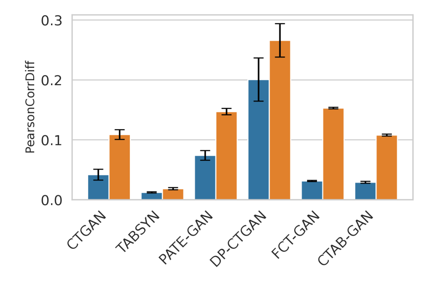
(a) Pearson Correlation Difference

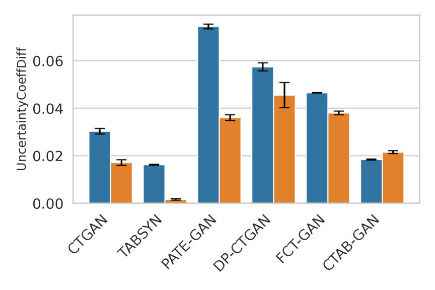
(b) Uncertainty Coefficient Difference

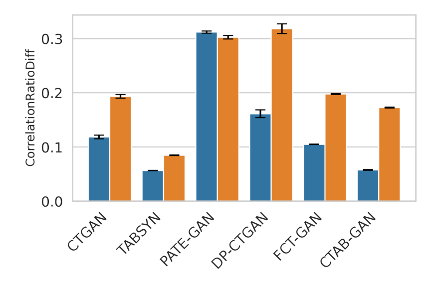
(c) Correlation Ratio Difference

Figure 8. Comparison of feature dependency metrics.

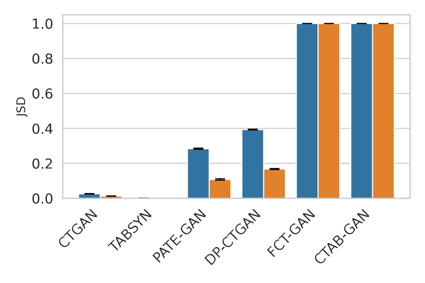
(a) Jensen-Shannon Divergence

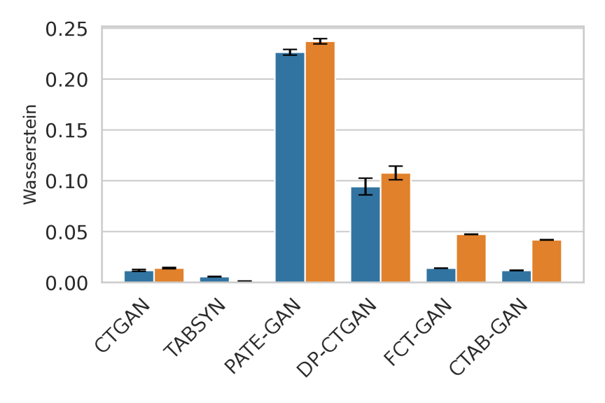
(b) Wasserstein Distance

Figure 9. Comparison of statistical similarity by model and dataset.

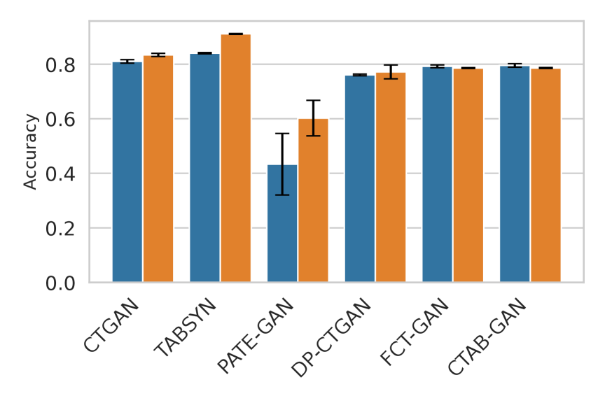
(a) Model Inversion Attack - Accuracy

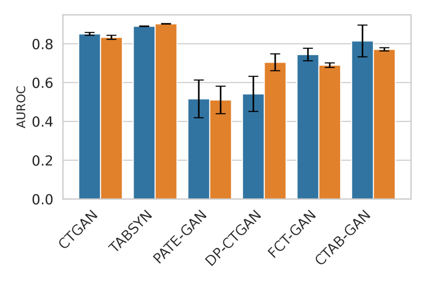
(b) Model Inversion Attack - AUROC

Figure 10. Comparison of Privacy metrics by model and dataset.

Comparison of Privacy metrics by model and dataset.

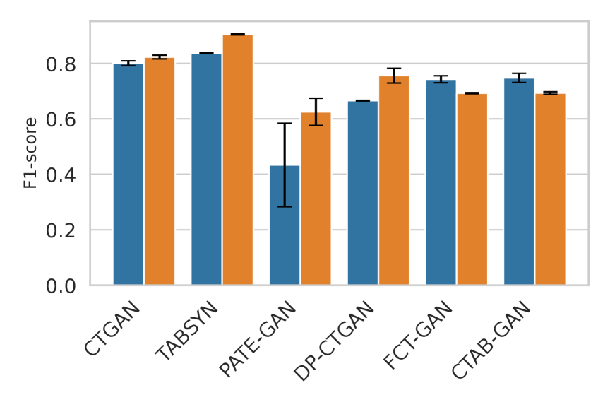
(a) F1-Score

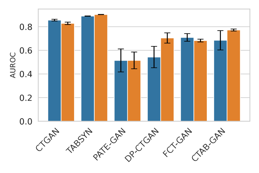
(b) AUROC

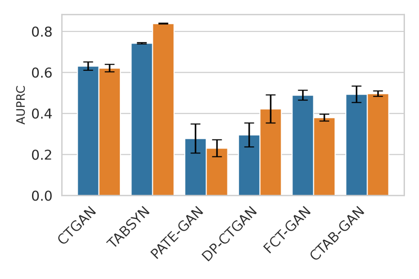
(c) AUPRC

(d) Accuracy

Figure 11. Machine Learning Utility Metrics by model and dataset.

Machine Learning Utility Metrics by model and dataset.

To assess how well synthetic data retains feature dependencies, we compare real and synthetic data using three metrics: Pearson Correlation Difference (for continuous features), Uncertainty Coefficient Difference (for categorical features), and Correlation Ratio Difference (for mixed feature pairs). Smaller differences indicate higher structural fidelity. Across both the Adult and CreditRisk datasets, Figure 8 shows that TABSYN achieves the lowest deviations across all three metrics, particularly excelling on the Credit dataset with correlation differences as low as 0.012–0.056. Moreover, the associated p-values for TABSYN are above 0.09, indicating that these differences are not statistically significant and thus the synthetic data closely preserves the real data relationships. In contrast, models such as PATE-GAN and DP-CTGAN exhibit substantially larger correlation differences up to 0.27 for Pearson’s correlation and 0.32 for correlation ratio differences with highly significant p-values ($p=0.002$). This demonstrates statistically robust distortions likely introduced by the noise added for privacy guarantees. These models also show greater variability (standard deviation), particularly DP-CTGAN, indicating inconsistent synthetic data quality across runs. Models like CTGAN, FCT-GAN, and CTAB-GAN generally achieve moderate fidelity with smaller but statistically significant distortions, reflected by correlation differences around 0.03–0.11 and low variance.

We further evaluate distributional similarity using Jensen-Shannon Divergence (JSD) for categorical features and Wasserstein Distance for continuous features. Figure 9 demonstrates that TABSYN consistently attains near-zero JSD and Wasserstein distances (e.g., JSD as low as 0.0000 on CreditRisk and Wasserstein distance below 0.006), with non-significant p-values ($p>0.09$). This confirms a strong match between synthetic and real data distributions. Conversely, FCT-GAN and CTAB-GAN exhibit maximum JSD values of 1.0 on both datasets with significant p-values ($p=0.002$), signaling extreme divergence in categorical distributions despite moderate Wasserstein distances. These findings suggest some models produce samples that appear realistic superficially, but deviate substantially in underlying distributional properties.

Privacy leakage is evaluated through vulnerability to model inversion attacks, where higher Accuracy and AUROC reflect greater privacy risk. Figure 10 summarizes the results across all models. TABSYN and CTGAN are most vulnerable, with AUROC scores reaching 0.89 on Adult and 0.90 on CreditRisk datasets ($p=0.002$). This indicates adversaries can reliably distinguish training samples, revealing potential overfitting. In contrast, privacy-focused models PATE-GAN and DP-CTGAN demonstrate AUROC values close to random guessing (approximately 0.50), confirming effective mitigation of privacy risks at the expense of fidelity.

To quantify downstream utility, classifiers trained on synthetic data are evaluated on real data using F1-score, AUROC, AUPRC, and Accuracy. Figure  11 presents the results across all models and datasets. CTAB-GAN consistently delivers strong performance across all metrics and datasets, achieving F1-scores around 0.74–0.75 and Accuracy near 0.79–0.78, with statistically significant differences ($p=0.002$) relative to baseline. FCT-GAN also performs well on the Adult dataset but shows moderate utility decline on CreditRisk. Although TABSYN attains the highest F1-scores (up to 0.90), its AUROC and AUPRC metrics decline notably on Adult, with p-values near 0.09 indicating these differences are not significant but suggest a tendency toward overfitting or reduced ranking robustness. On the other hand, DP-CTGAN and PATE-GAN suffer from substantially degraded utility across both datasets (e.g., Accuracy as low as 0.43 and AUROC near 0.51 on Adult), consistently with significant p-values ($p=0.002$). This underscores the classical privacy-utility tradeoff, where privacy preservation reduces the usefulness of synthetic data for predictive modeling. Additionally, these models show higher performance variability, reflecting unstable training dynamics under differential privacy constraints.

Overall, model performance varies markedly between datasets. The CreditRisk dataset, being more complex with higher feature dimensionality and imbalance, presents greater challenges for synthetic data generation. This results in larger fidelity and utility losses, particularly for privacy-preserving models. Therefore, model selection should be informed by dataset characteristics and the desired balance between privacy, fidelity, and utility. The full experimental pipeline and code are publicly available at https://github.com/Raju-Challagundla/syndataeval.

5. Challenges & Limitations

While significant progress has been made in the generation of synthetic data for tabular data, several challenges remain unresolved. A primary concern is balancing privacy guarantees with data utility. Techniques such as differential privacy and secure multi-party computation aim to preserve privacy but do not entirely eliminate the risk of model inversion attacks. These attacks enable adversaries to infer sensitive information, particularly when synthetic data closely approximates the original distribution. In regulated industries like finance and healthcare, where privacy laws such as GDPR and HIPAA mandate strict data handling protocols, achieving an optimal trade-off between privacy and utility is especially challenging. Frequent policy changes and data deletion requests further complicate dataset stability, leading to incomplete or inconsistent data. This instability degrades machine learning model performance, often resulting in biased or unrealistic predictions.

Another critical limitation is the generalizability of synthetic data models across diverse datasets. Real-world data spans a wide range of applications, each with unique statistical properties, feature interactions, and domain-specific characteristics. Models that perform well on one dataset often struggle with others, raising concerns about the scalability of existing methods. As industries evolve and incorporate new data types, ensuring that synthetic data models remain adaptable is an ongoing challenge.

A more complex issue is the accurate preservation of feature dependencies. Many domains involve intricate relationships between variables, such as correlations, temporal patterns, or hierarchical structures. High-dimensional or sequential data further complicates dependency modeling, as inaccuracies can lead to unrealistic synthetic outputs. This undermines the reliability of synthetic data for downstream tasks such as predictive modeling and decision making. In addition, imbalanced data sets, particularly those where rare events are critical, pose significant difficulties. The failure to capture these rare but important occurrences can render synthetic data ineffective in real-world applications.

Ensuring statistical fidelity and realism remains a central challenge. While advanced generative models, including GANs, VAEs, and diffusion models, have made notable progress, they still struggle to fully replicate the nuanced distributions and dependencies found in real-world data. Achieving realism requires models to capture complex variable relationships without overfitting to specific datasets. Furthermore, these models must continuously adapt to evolving data landscapes, including new features, shifting conditions, and emerging trends.

The evaluation of synthetic data also presents a significant limitation. Currently, there is no consensus on comprehensive, domain-specific metrics for assessing synthetic data quality. Traditional measures, such as distributional similarity or diversity, may not fully reflect the utility of synthetic data in high-stakes applications. The absence of standardized evaluation frameworks makes it difficult to determine whether synthetic data can reliably replace real data in critical tasks.

Lastly, the interpretability of generative models remains a barrier to adoption. Many state-of-the-art models, such as GANs and VAEs, operate as black boxes, making it difficult for practitioners to understand the underlying generation process. In industries where decisions have substantial consequences, stakeholders may be hesitant to trust synthetic data produced by opaque systems.

Appendices

Appendix A Definitions in Literature

Table A.5. Examples of Synthetic Data Generation Definitions in prior literature

Source	Definition
Bishop (2006) (Bishop and Nasrabadi, 2006)	Discusses probabilistic modeling and density estimation, which serve as the foundation for synthetic data generation. The goal is to approximate the underlying distribution of real data $\mathbf{X}$ using a model $\hat{P}(\mathbf{X})$ and generate synthetic samples $Y$ by drawing from this estimated distribution: $$\mathbf{X}_{\text{syn}}\sim\hat{P}(\mathbf{X}).$$ This approach includes parametric and non-parametric methods to learn $\hat{P}(\mathbf{X})$.
Goodfellow et al. (2014) (Goodfellow et al., 2014)	Emphasizes the use of Generative Adversarial Networks (GANs), where a generator network $G$ maps random noise $Z\sim P(Z)$ to synthetic data $X_{\text{syn}}$, and a discriminator network $D$ evaluates its authenticity. The iterative training process refines the synthetic data distribution $\hat{P}(X)$ to closely approximate the original data distribution $P(X)$. This process is mathematically represented as: $$\mathbf{X}_{\text{syn}}\sim\hat{P}(\mathbf{X}).$$ The adversarial training objective is given by: $$\min_{G}\max_{D}\mathbb{E}_{X\sim P(X)}[\log D(X)]+\mathbb{E}_{Z\sim P(Z)}[\log(1-D(G(Z)))].$$ Through this process, the generator learns to produce synthetic samples that are statistically similar to real data, ensuring that $\hat{P}(\mathbf{X})\approx P(\mathbf{X})$.
Kingma & Welling (2013) (Kingma and Welling, 2013)	Introduces Variational Autoencoders (VAEs), which generate synthetic data by learning a probabilistic mapping between latent variables $\mathbf{Z}$ and observations $\mathbf{X}$. Given a prior $p(\mathbf{Z})$, synthetic samples are drawn as follows: $$\mathbf{Z}\sim\mathcal{N}(\mathbf{0},\mathbf{I}),\quad\mathbf{X}_{\text{syn}}\sim p(\mathbf{X}\mid\mathbf{Z}).$$ where $p(\mathbf{X}\mid\mathbf{Z})$ is a probability density function and $\mathbf{Z}$ is a latent variable. The objective is to maximize the evidence lower bound (ELBO) to approximate $P(\mathbf{X})$ via $p(\mathbf{X}\mid\mathbf{Z})$.
Reynolds (2009) (Reynolds et al., 2009)	Discusses synthetic data generation using Gaussian Mixture Models (GMMs), where the original data’s distribution is approximated by a mixture of Gaussians. The synthetic data is generated by sampling from this mixture model: $$P(\mathbf{X})=\sum_{k=1}^{K}\pi_{k}\mathcal{N}(\mathbf{X}\mid\mu_{k},\Sigma_{k}).$$ where $\pi_{k}$ are the mixture weights, and $\mathcal{N}(\mathbf{X}\mid\mu_{k},\Sigma_{k})$ represents the Gaussian component with mean $\mu_{k}$ and covariance $\Sigma_{k}$. The synthetic data is then sampled as: $$\mathbf{X}_{\text{syn}}\sim\hat{P}(\mathbf{X})=\sum_{k=1}^{K}\hat{\pi}_{k}\mathcal{N}(\mathbf{X}\mid\hat{\mu}_{k},\hat{\Sigma}_{k}).$$ where $\hat{\pi}_{k},\hat{\mu}_{k},$ and $\hat{\Sigma}_{k}$ are estimated from the original data distribution.
Rabiner (1989) (Rabiner, 1989)	Synthetic data generation for sequential data can be achieved using Hidden Markov Models (HMMs), where sequences are modeled probabilistically as a series of hidden states and observed outputs. The synthetic sequences are generated by sampling from the estimated HMM parameters: $$P(\mathbf{X},S)=P(S_{1})\prod_{t=2}^{T}P(S_{t}\mid S_{t-1})P(\mathbf{X}_{t}\mid S_{t}).$$ where $S_{t}$ is the hidden state at time $t$, and $\mathbf{X}_{t}$ is the observed output. The synthetic sequence is then generated as: $$\mathbf{X}_{\text{syn}}\sim\hat{P}(\mathbf{X})=\hat{P}(S_{1})\prod_{t=2}^{T}\hat{P}(S_{t}\mid S_{t-1})\hat{P}(\mathbf{X}_{t}\mid S_{t}).$$ where $\hat{P}(S_{t}\mid S_{t-1})$ and $\hat{P}(\mathbf{X}_{t}\mid S_{t})$ are the estimated transition and emission probabilities, respectively. This ensures that $\hat{P}(\mathbf{X})$ approximates $P(\mathbf{X})$, generating realistic sequential synthetic data.

Appendix B Synthetic Data Generation

In the era of big data (Council, 2023), generating synthetic data has become a crucial technique in various fields such as data privacy, machine learning, and statistical analysis. Synthetic data helps in creating large datasets like credit risk data (Kaggle, nd), facilitates model training when real data is scarce, and aids in understanding and validating statistical models. This section provides an overview of generative models and statistical models that are foundational for synthetic data generation. While generative models leverage neural architectures to learn complex data distributions and generate realistic samples, statistical models rely on probabilistic techniques to capture underlying structures in data. This distinction highlights the methodological differences in generating synthetic data, balancing realism and interpretability.

B.1. Generative Models

Generative models aim to learn the underlying distribution of a dataset and can generate new data points that resemble the training data. These models are particularly valuable in situations where acquiring real data is difficult, expensive, or raises privacy concerns (Syntho.ai, 2023; Gretel.ai, 2023; Syntheticus.ai, 2023). By capturing the essential features and patterns of the data, generative models can produce high-quality synthetic samples that maintain the statistical properties of the original dataset.

A generative model $G$ is a model that learns the underlying data distribution and generates new samples that resemble the original data. Formally, given a generative model $G$, it produces synthetic data points

$$\mathbf{X}_{\text{syn}}=\{\mathbf{x}^{\prime}_{i}\in\mathbb{R}^{p}\mid i=1,2,\ldots,n\},$$

where each sample $\mathbf{x}^{\prime}_{i}$ is drawn from the learned distribution, i.e., $\mathbf{x}^{\prime}_{i}\sim G$.

B.1.1. Autoencoders and Variational Autoencoders (VAEs)

Autoencoders (Kingma and Welling, 2013) are a type of neural network that encode data into a latent space and then reconstruct it back to the original input. The process can be mathematically represented as follows:

$$\mathbf{h}=f_{\text{enc}}(\mathbf{x}),$$

$$\mathbf{x}^{\prime}=f_{\text{dec}}(\mathbf{h}),$$

where $f_{\text{enc}}$ and $f_{\text{dec}}$ are the encoder and decoder functions, respectively. The encoder compresses the input data $\mathbf{x}$ into a lower-dimensional representation $\mathbf{h}$, while the decoder attempts to reconstruct the original data from this representation. Figure 12(a) illustrates the structure of a standard Autoencoder (AE), where the latent code $\mathbf{h}$ serves as a bottleneck that forces the model to learn compact feature representations.

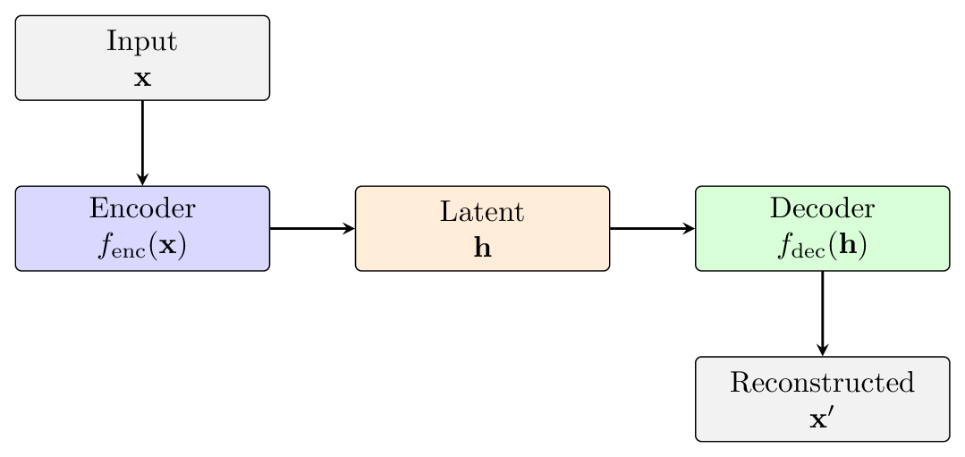
(a) Autoencoder

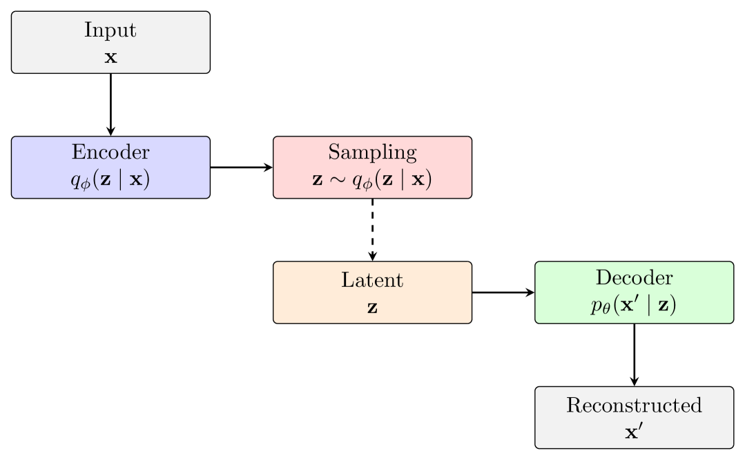
(b) Variational Autoencoder

Figure 12. (a) A standard Autoencoder encodes the input into a deterministic latent representation $\mathbf{h}$ before reconstructing it. (b) A Variational Autoencoder (VAE) introduces a probabilistic latent space, where the encoder maps the input into a distribution over possible latent representations.

Variational Autoencoders (VAEs) (Kingma and Welling, 2013) extend the concept of traditional autoencoders by introducing a probabilistic approach to the latent space. Instead of mapping inputs to a fixed latent code $\mathbf{h}$, VAEs learn a distribution over latent variables $\mathbf{z}$. As depicted in Figure 12(b), rather than directly outputting a single latent vector, the encoder produces parameters for a probability distribution:

$$q_{\phi}(\mathbf{z}\mid\mathbf{x})=\mathcal{N}(\boldsymbol{\mu},\boldsymbol{\sigma}^{2}\mathbf{I}),$$

where $\boldsymbol{\mu}$ and $\boldsymbol{\sigma}^{2}$ represent the learned mean and variance of the distribution. Instead of using $\mathbf{h}$ deterministically, VAEs sample $\mathbf{z}$ from the encoded distribution:

$$\mathbf{z}\sim\mathcal{N}(\boldsymbol{\mu},\boldsymbol{\sigma}^{2}).$$

The decoder then reconstructs the data by mapping $\mathbf{z}$ back to the data space through a likelihood function:

$$p_{\theta}(\mathbf{x}^{\prime}\mid\mathbf{z})\approx\mathcal{N}(f_{\text{dec}}(\mathbf{z}),\sigma^{2}\mathbf{I}).$$

The use of a probabilistic latent space allows VAEs to generate diverse samples by drawing from different points in the learned distribution, rather than relying on a single deterministic encoding as in standard Autoencoders.

The training objective of VAEs maximizes the Evidence Lower Bound (ELBO), which consists of two key terms:

1. Reconstruction Loss – Ensuring that $\mathbf{x}^{\prime}$ closely resembles the original input $\mathbf{x}$.

2. Regularization Term – Encouraging $q_{\phi}(\mathbf{z}\mid\mathbf{x})$ to be close to a prior distribution $p(\mathbf{z})$, typically a standard Gaussian:

   $$p(\mathbf{z})=\mathcal{N}(\mathbf{0},\mathbf{I}).$$

By enforcing this constraint, VAEs ensure that the latent space remains structured and meaningful, making them particularly effective for generative tasks such as image synthesis and anomaly detection.

B.1.2. Generative Adversarial Networks (GANs)

Generative Adversarial Networks (GANs) (Goodfellow et al., 2014) are a revolutionary framework in machine learning that consists of two neural networks: a generator $\mathbf{G}$ and a discriminator $\mathbf{D}$. The generator is responsible for creating synthetic data, while the discriminator evaluates the authenticity of the data, distinguishing between real data and the data generated by the generator. The relationship between the generator and the noise input can be expressed as:

(9) $$\mathbf{x^{\prime}}=\mathbf{G}(\mathbf{z};\theta_{\mathbf{G}}),$$

where $\mathbf{z}$ is a noise vector and $\theta_{\mathbf{G}}$ are the generator parameters (Goodfellow et al., 2014). The generator $\mathbf{G}$ learns to transform noise $\mathbf{z}$ into synthetic data $\mathbf{x^{\prime}}$ that resembles the real data $\mathbf{X}$, while the discriminator $\mathbf{D}$ tries to distinguish between real $\mathbf{x}$ and generated $\mathbf{x^{\prime}}$. Figure 13 illustrates the architecture of a typical GAN, showing the interaction between the generator and discriminator during the learning process. The figure highlights the flow of data from the noise vector $\mathbf{z}$ to the generator $\mathbf{G}$, the generation of synthetic data $\mathbf{x^{\prime}}$, and the discriminator $\mathbf{D}$’s role in classifying real and generated data. GANs are trained using an adversarial objective to find an equilibrium:

(10) $$\min_{\mathbf{G}}\max_{\mathbf{D}}\mathbb{E}_{\mathbf{x}\sim p_{\text{data}}(\mathbf{x})}[\log\mathbf{D}(\mathbf{x})]+\mathbb{E}_{\mathbf{z}\sim p_{\mathbf{z}}(\mathbf{z})}[\log(1-\mathbf{D}(\mathbf{G}(\mathbf{z})))].$$

Here,

(11) $$\mathbb{E}_{\mathbf{x}\sim p_{\text{data}}(\mathbf{x})}[\log\mathbf{D}(\mathbf{x})]$$

represents the log-probability that the discriminator correctly classifies real data $\mathbf{x}$, and

(12) $$\mathbb{E}_{\mathbf{z}\sim p_{\mathbf{z}}(\mathbf{z})}[\log(1-\mathbf{D}(\mathbf{G}(\mathbf{z})))]$$

represents the log-probability that the discriminator correctly classifies generated data $\mathbf{G}(\mathbf{z})$ (Goodfellow et al., 2014). The adversarial training process is visually summarized in Figure 13, which also includes the generator and discriminator losses.

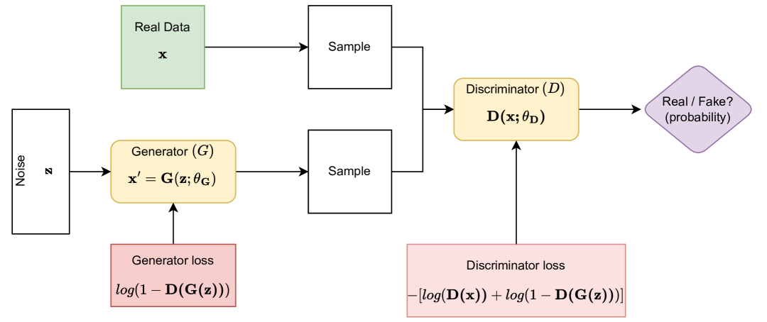
Figure 13. Architecture of a Generative Adversarial Network (GAN). The generator $\mathbf{G}$ transforms noise $\mathbf{z}$ into synthetic data $\mathbf{x^{\prime}}$, while the discriminator $\mathbf{D}$ distinguishes between real data $\mathbf{x}$ and generated data $\mathbf{x^{\prime}}$. The generator minimizes Eq. (11), and the discriminator minimizes Eq. (12).

The training process of Generative Adversarial Networks (GANs) involves an iterative optimization of two neural networks: the generator $\mathbf{G}$ and the discriminator $\mathbf{D}$. Initially, the parameters of both networks are randomly initialized. In each training iteration, a batch of real data is sampled from the training dataset, while a batch of noise vectors is drawn from a predefined prior distribution, such as a Gaussian distribution. The generator then transforms these noise vectors into synthetic data samples, denoted as Eq.(9). The discriminator is updated by optimizing a loss function that encourages it to correctly classify real data as authentic and generated data as synthetic Eq.(10). Simultaneously, the generator is updated by minimizing an objective that pushes it to generate more realistic samples, effectively fooling the discriminator Eq.(11). This adversarial process continues iteratively until convergence, where the generator produces synthetic data that closely resembles the real distribution while the discriminator struggles to distinguish between real and generated samples, as demonstrated in foundational studies on GANs (Goodfellow et al., 2014). The interplay between the generator and discriminator is visually depicted in Figure 13, which provides a clear representation of the GAN architecture and training process. GANs have gained significant attention for their ability to generate high-quality synthetic data, making them a powerful tool in various applications, including image generation, video synthesis, and more.

B.1.3. Diffusion Models

Diffusion models are a class of generative models that progressively add noise to data and then learn how to reverse this noising process to generate new samples. The process is defined by two main phases: the forward (noising) process and the reverse (denoising) process (Ho et al., 2020).

Let $\mathbf{x}_{0}\in\mathbb{R}^{p}$ be the original data point (e.g., an image or tabular data point). The forward process is a Markov chain that gradually adds Gaussian noise over a series of $T$ steps. The forward process at step $t$ is defined as:

$$\mathbf{x}_{t}=\sqrt{\alpha_{t}}\mathbf{x}_{t-1}+\sqrt{1-\alpha_{t}}\mathbf{\epsilon}_{t},\quad t=1,2,\dots,T,$$

where $\mathbf{\epsilon}_{t}\sim\mathcal{N}(0,I)$ is standard Gaussian noise, and $\alpha_{t}$ is a scaling factor that controls the amount of noise added at each step (Ho et al., 2020). The process continues until $t=T$, at which point the data is completely noisy and approximately follows a standard normal distribution $\mathbf{x}_{T}\sim\mathcal{N}(0,I)$.

The reverse process is the core of the diffusion model. Given the noisy data $\mathbf{x}_{T}$, the goal is to reverse the noising process and recover data that resembles the original distribution. The reverse process is parameterized by a neural network and is given by:

$$p_{\theta}(\mathbf{x}_{t-1}\mid\mathbf{x}_{t})=\mathcal{N}(\mathbf{x}_{t-1};\mu_{\theta}(\mathbf{x}_{t},t),\Sigma_{\theta}(\mathbf{x}_{t},t)),$$

where $\mu_{\theta}(\mathbf{x}_{t},t)$ and $\Sigma_{\theta}(\mathbf{x}_{t},t)$ are the mean and variance predicted by the model at each step $t$, and the neural network learns to reverse the forward process.

The objective of training a diffusion model is to minimize the Kullback-Leibler (KL) divergence between the true reverse process $q(\mathbf{x}_{t-1}\mid\mathbf{x}_{t},\mathbf{x}_{0})$ and the learned reverse process $p_{\theta}(\mathbf{x}_{t-1}\mid\mathbf{x}_{t})$. The loss function is defined as:

(13) $$\mathcal{L}=\mathbb{E}_{q(\mathbf{x}_{0},\mathbf{x}_{1},\dots,\mathbf{x}_{T})}\left[\sum_{t=1}^{T}\text{KL}(q(\mathbf{x}_{t-1}\mid\mathbf{x}_{t},\mathbf{x}_{0})\|p_{\theta}(\mathbf{x}_{t-1}\mid\mathbf{x}_{t}))\right],$$

where $q(\mathbf{x}_{t-1}\mid\mathbf{x}_{t},\mathbf{x}_{0})$ is the true posterior distribution, and $p_{\theta}(\mathbf{x}_{t-1}\mid\mathbf{x}_{t})$ is the model’s learned reverse process (Ho et al., 2020; Song et al., 2020a). Once the model is trained, synthetic data can be generated by starting from random noise $\mathbf{x}_{T}\sim\mathcal{N}(0,I)$ and applying the learned reverse process to iteratively denoise the data:

$$\mathbf{x^{\prime}}_{i}=\hat{\mathbf{x}}_{T}\to\hat{\mathbf{x}}_{T-1}\to\dots\to\hat{\mathbf{x}}_{1}\to\hat{\mathbf{x}}_{0}=G(z),$$

where $G(z)$ denotes the generative process starting from random noise $z$, and $\hat{\mathbf{x}}_{t}$ represents the denoised data at each step. The final generated data point $\mathbf{x^{\prime}}_{i}$ approximates the original data distribution after applying the reverse diffusion steps (Song et al., 2020a). This iterative process allows the model to learn to generate high-quality synthetic data that resembles the real data distribution. Figure 14 illustrates the forward and reverse processes in diffusion models.

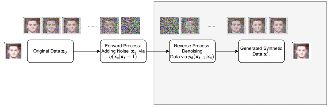
Figure 14. Illustration of the Diffusion Process: The forward process adds noise to the data progressively, while the reverse process denoises it to generate synthetic data. The process begins with original data $\mathbf{x}_{0}$ and ends with the generated data $\mathbf{x^{\prime}}_{i}$.

B.1.4. Autoregressive Models

Autoregressive generative models, initially developed for tasks such as language modeling (Radford, 2018), have gained traction in the domain of synthetic data generation, particularly for structured tabular data. These models generate data sequentially, producing each feature conditioned on the previously generated ones. This formulation allows them to capture complex dependencies between features, which is essential in tabular data where relationships are often non-linear and cross-dimensional (Hoogeboom et al., 2021a).

Formally, the generative process is defined as:

$$\mathbf{x}^{\prime}_{i}=G(\mathbf{x}_{<i};\theta_{G}),$$

where $\mathbf{x}_{<i}=(\mathbf{x}^{\prime}_{1},\mathbf{x}^{\prime}_{2},\dots,\mathbf{x}^{\prime}_{i-1})$ denotes the sequence of previously generated features, $\mathbf{x}^{\prime}_{i}$ is the feature being generated at step $i$, and $\theta_{G}$ are the parameters of the generative model. The full synthetic data sample is then constructed as:

$$\mathbf{x}^{\prime}=(\mathbf{x}^{\prime}_{1},\mathbf{x}^{\prime}_{2},\dots,\mathbf{x}^{\prime}_{n}).$$

These models are typically trained using maximum likelihood estimation (MLE), optimizing the negative log-likelihood (NLL) over the training data:

$$\mathcal{L}=-\sum_{i=1}^{n}\log P(\mathbf{x}_{i}\mid\mathbf{x}_{<i};\theta_{G}),$$

where $P(\mathbf{x}_{i}\mid\mathbf{x}_{<i};\theta_{G})$ represents the conditional probability of the $i$-th feature given the previous ones. This objective encourages the model to accurately learn and replicate the statistical dependencies within the dataset.

This autoregressive formulation aligns naturally with the Transformer architecture (Vaswani et al., 2017), which relies on self-attention mechanisms to model dependencies across input positions. By applying causal (masked) self-attention, Transformers ensure that the prediction at position $i$ is conditioned only on positions $<i$, thereby maintaining the autoregressive property. This makes them especially well-suited for tasks like synthetic tabular data generation, where feature dependencies can be highly non-linear and sparse (Huang et al., 2020). A Transformer-based autoregressive model for synthetic tabular data generation typically incorporates the following core components:

Input Embedding: Each feature, whether categorical or numerical, is mapped into a high-dimensional space using embeddings. For numerical features, this is achieved through a linear transformation:

$$\mathbf{E(x)}=W_{e}\mathbf{x},$$

where $W_{e}$ is the embedding weight matrix. For categorical features, separate embeddings are learned:

$$\mathbf{E_{\text{cat}}(x)}=W_{c}\mathbf{x}.$$

Positional Encoding: Since Transformers do not inherently encode the order of features, positional encodings are added to retain information about the sequence of features. The positional encoding for the $i$-th feature is computed as:

$$\mathbf{PE(x)_{i}}=\sin\left(\frac{i}{10000^{2j/d}}\right),\quad\mathbf{PE(x)_{i+1}}=\cos\left(\frac{i}{10000^{2j/d}}\right),$$

where $d$ is the dimensionality of the embeddings.

Multi-Head Self-Attention: The self-attention mechanism captures dependencies between features by computing queries ($\mathbf{Q}$), keys ($\mathbf{K}$), and values ($\mathbf{V}$):

$$\mathbf{Q}=W_{Q}\mathbf{E(x)},\quad\mathbf{K}=W_{K}\mathbf{E(x)},\quad\mathbf{V}=W_{V}\mathbf{E(x)}.$$

The attention scores are computed as:

(14) $$\text{Attention}(\mathbf{Q},\mathbf{K},\mathbf{V})=\text{softmax}\left(\frac{\mathbf{QK}^{T}}{\sqrt{d_{k}}}\right)\mathbf{V},$$

where $d_{k}$ is the dimensionality of the keys. Multi-head attention extends this by computing multiple attention scores in parallel and concatenating the results.

Feedforward Network: After the self-attention layer, each feature representation is passed through a feedforward neural network:

$$\mathbf{x^{\prime}}=\sigma(W_{2}\text{ReLU}(W_{1}\mathbf{x})),$$

where $W_{1}$ and $W_{2}$ are learnable weight matrices, and $\sigma$ is a non-linear activation function.

Autoregressive Generation: The final step involves generating each feature sequentially. The probability distribution for the $i$-th feature is computed as:

$$P(\mathbf{x_{i}}|\mathbf{x_{<i}})=\text{softmax}(W_{o}h_{i}),$$

where $h_{i}$ is the hidden representation of the $i$-th feature, and $W_{o}$ is the output weight matrix. This integrated autoregressive design enables Transformer models to generate synthetic tabular data feature-by-feature, capturing both linear and non-linear dependencies in the order defined during training. Refer to Figure 15 for a visual representation of the autoregressive Transformer-based generation process.

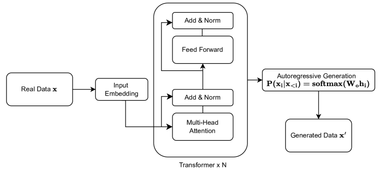
Figure 15. Architecture of a Transformer-based Synthetic Data Generator. The model processes input features through embeddings and positional encodings, applies self-attention to capture dependencies, and generates synthetic samples autoregressively.

B.1.5. Masked Generative Models

Masked generative models are a class of models that learn to model the data distribution by predicting missing or masked features conditioned on the observed ones. These models iteratively mask and reconstruct portions of the data, enabling them to capture complex feature dependencies in high-dimensional data such as tabular datasets (Ma et al., 2018; Yoon et al., 2018).

Let $\mathbf{x}=(x_{1},x_{2},\dots,x_{p})\in\mathbb{R}^{p}$ denote a data sample with $p$ features. A random binary mask $\mathbf{m}\in\{0,1\}^{p}$ indicates which features are observed ($m_{j}=1$) and which are masked ($m_{j}=0$). The model is trained to predict the masked features $\mathbf{x}_{\text{mask}}$ given the observed ones $\mathbf{x}_{\text{obs}}$, by maximizing the conditional likelihood:

$$\log p_{\theta}(\mathbf{x}_{\text{mask}}\mid\mathbf{x}_{\text{obs}}),$$

where $\theta$ represents the model parameters.

During training, the model learns to infer missing values across different masking patterns by minimizing the reconstruction loss:

$$\mathcal{L}=\mathbb{E}_{\mathbf{x},\mathbf{m}}\left[\|\mathbf{x}_{\text{mask}}-f_{\theta}(\mathbf{x}_{\text{obs}},\mathbf{m})\|^{2}\right],$$

where $f_{\theta}$ is a neural network that predicts the masked entries. In practice, the masking pattern is varied across training samples to encourage the model to learn dependencies among all features (Ma et al., 2018). Once trained, synthetic data can be generated in an autoregressive or iterative fashion. For instance, one may begin with an empty or partially filled vector $\hat{\mathbf{x}}$, and iteratively sample unobserved features conditioned on previously generated ones:

$$\hat{x}_{j}\sim p_{\theta}(x_{j}\mid\hat{x}_{1},\dots,\hat{x}_{j-1}),$$

where the feature ordering can be fixed or learned dynamically. Alternatively, masked models can perform Gibbs sampling-like generation by repeatedly masking and imputing values over several iterations until convergence (Yoon et al., 2018).

These models are particularly suited for tabular data because they can handle mixed data types, missingness, and heterogeneous feature correlations. Notable examples include GAIN (Generative Adversarial Imputation Nets) (Yoon et al., 2018) and more recent approaches such as MICE-style transformers like MaskGIT (Chang et al., 2022). Figure 16 shows an illustration of the masked generation process.

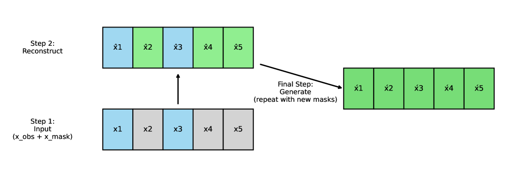
Figure 16. Illustration of the masked generative modeling process. A binary mask separates observed (blue) and masked (gray) features. The model is trained to predict the masked values (shown in green) conditioned on the observed ones using a reconstruction loss. During generation, synthetic samples are produced by iteratively imputing masked features, starting from an empty or partially observed vector, and repeating the process with new masks until a complete sample is formed.

B.2. Statistical Models

Statistical models aim to capture the statistical properties and dependencies within data by approximating the distributions and relationships observed in real datasets. These models assume a specific form for the data distribution, characterized by a finite set of parameters, and focus on estimating these parameters to define the distribution. By leveraging such assumptions, they provide a structured and efficient approach to modeling data, which is particularly valuable in synthetic data generation. Controlling the distribution and dependencies of generated data is crucial, making these models well-suited for this purpose. Commonly used statistical models in synthetic data generation include Bayesian Networks (BNs) (Pearl, 2014), Gaussian Mixture Models (GMMs) (Bishop and Nasrabadi, 2006; Reynolds et al., 2009), and Hidden Markov Models (HMMs) (Rabiner, 1989). These models enable efficient parameter estimation and sampling, facilitating the generation of large amounts of synthetic data while preserving statistical properties such as correlations and distributions.

B.2.1. Bayesian Networks

Bayesian Networks (BNs) (Pearl, 2014) are powerful probabilistic models used for modeling dependencies among a set of variables, making them useful for generating synthetic data. These networks represent conditional dependencies through a directed acyclic graph (DAG) (Bishop and Nasrabadi, 2006), where nodes represent random variables and edges represent conditional dependencies between these variables.

Let $\mathbf{X=\{X_{1},X_{2},\dots,X_{n}\}}$ represent a set of real-world variables (data features). A Bayesian network defines the joint distribution $P(\mathbf{X})$ of these variables by decomposing it into a product of conditional distributions based on the structure of the network:

(15) $$\mathbf{P(X)=\prod_{i=1}^{n}P(\mathbf{X}_{i}\mid\text{Pa}(\mathbf{X}_{i}))}$$

where $\text{Pa}(\mathbf{X}_{i})$ represents the set of parent variables for node $\mathbf{X}_{i}$ in the DAG.

To generate synthetic data $\mathbf{X_{\text{syn}}}$ using a Bayesian network, the process typically involves the following steps.

Parameter Estimation: First, a Bayesian network is learned from the real data $\mathbf{X}$ using parameter estimation techniques. This involves estimating the conditional probability distributions (CPDs) $\mathbf{P(X_{i}}\mid\text{Pa}(\mathbf{X}_{i}))$ for all nodes based on the observed data.

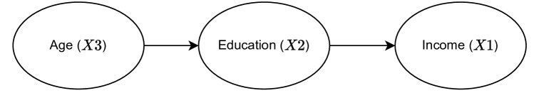
Figure 17. A simple Bayesian network showing the dependencies between age ($\mathbf{X}_{3}$), education ($\mathbf{X}_{2}$), and income ($\mathbf{X}_{1}$).

For example, consider a network (Figure 17) with three variables: income ($\mathbf{X}_{1}$), education ($\mathbf{X}_{2}$), and age ($\mathbf{X}_{3}$). The relationships between these variables can be captured using CPDs such as

$$\mathbf{X_{1}\mid X_{2}\sim\mathcal{N}(\mu_{1},\sigma_{1}^{2})},$$

where income $\mathbf{X}_{1}$ is conditionally dependent on education $\mathbf{X}_{2}$, with a Gaussian distribution. Similarly,

$$\mathbf{X_{2}\mid X_{3}\sim\mathcal{N}(\mu_{2},\sigma_{2}^{2})},$$

where education $\mathbf{X}_{2}$ is conditionally dependent on age $\mathbf{X}_{3}$, also modeled using a Gaussian distribution. Finally,

$$\mathbf{X_{3}\sim\text{Uniform}(a,b)},$$

where age $\mathbf{X}_{3}$ is assumed to follow a uniform distribution. These CPDs are estimated from the observed data, allowing the structure of the Bayesian network to reflect the dependencies between the variables.

Sampling: Once the parameters of the Bayesian network are estimated, synthetic data $\mathbf{X_{\text{syn}}}$ can be generated by sampling from the conditional distributions of each node $\mathbf{X}_{i}$. The process starts with the root nodes (nodes without parents). For instance, sample $\mathbf{X^{\prime}}_{3}$ from $P(\mathbf{X}_{3})$, the age distribution. Then, given the sampled value $\mathbf{X^{\prime}}_{3}$, sample $\mathbf{X^{\prime}}_{2}$ from the conditional distribution $P(\mathbf{X}_{2}\mid\mathbf{X^{\prime}}_{3})$, which represents the education distribution conditioned on the sampled age. Finally, given $\mathbf{X^{\prime}}_{2}$, sample $\mathbf{X^{\prime}}_{1}$ from $P(\mathbf{X}_{1}\mid\mathbf{X^{\prime}}_{2})$, the income distribution conditioned on the sampled education:

$$\mathbf{X^{\prime}_{3}\sim P(X_{3})},$$

$$\mathbf{X^{\prime}_{2}\sim P(X_{2}\mid X^{\prime}_{3})},$$

$$\mathbf{X^{\prime}_{1}\sim P(X_{1}\mid X^{\prime}_{2})}.$$

Iterative Sampling: This sampling process is repeated for all nodes in the network, following the structure of the directed acyclic graph (DAG). Each time the synthetic data is generated, the dependencies between the variables (age, education, and income) are preserved, ensuring that the synthetic dataset reflects the statistical relationships in the real data. After repeating this process for multiple instances, a synthetic dataset $\mathbf{X_{\text{syn}}}=\{\mathbf{X^{\prime}_{1},X^{\prime}_{2},X^{\prime}_{3}\}}$ would be generated, where each synthetic value corresponds to a feature in the real data $\mathbf{X=\{X_{1},X_{2},X_{3}\}}$.

B.2.2. Gaussian Mixture Models (GMM)

Gaussian Mixture Models (GMMs) (Bishop and Nasrabadi, 2006) are probabilistic models that represent a mixture of multiple Gaussian distributions. These models are widely used to model complex data that can be assumed to originate from several distinct Gaussian distributions. Each component in a GMM has its own mean and variance, and the data is assumed to be generated from a weighted sum of these Gaussian distributions.

The joint probability distribution $P(\mathbf{X})$ of a dataset $\mathbf{X=\{X_{1},X_{2},\dots,X_{n}}\}$ under a GMM is represented as a weighted sum of the individual Gaussian distributions:

$$\mathbf{P(X)}=\sum_{k=1}^{K}\boldsymbol{\pi}_{k}\mathcal{N}(\mathbf{X}\mid\boldsymbol{\mu}_{k},\boldsymbol{\sigma}_{k}^{2}),$$

where $\pi_{k}$ is the weight of the $k$-th Gaussian component, representing the proportion of the dataset generated by this component. $\mathcal{N}(\mathbf{X}\mid\mu_{k},\sigma_{k}^{2})$ is the Gaussian distribution with mean $\mu_{k}$ and variance $\sigma_{k}^{2}$. $K$ is the number of Gaussian components in the mixture (Reynolds et al., 2009).

Figure 18. A simple Gaussian Mixture Model with two Gaussian components. Data is modeled as a mixture of two Gaussian distributions. The blue curve represents the first Gaussian component with mean 0 and variance 1, while the red curve represents the second Gaussian component, centered at 2 with a variance of 1. The green curve represents the mixture of these two Gaussian components, with the blue component contributing 40% and the red component contributing 60% to the overall distribution.

GMMs are particularly advantageous because they do not require prior knowledge of the cluster assignments for the data points. Instead, they learn the parameters—means, covariances, and mixing coefficients—directly from the data $\mathbf{X}$. This flexibility allows GMMs to adapt to the inherent structure of the data, making them suitable for various applications, including clustering, density estimation, and anomaly detection. By generating synthetic data $\mathbf{X}^{\prime}$ that matches the statistical distribution of the original data $\mathbf{X}$, GMMs provide a robust framework for understanding and analyzing complex datasets. This capability is especially useful in scenarios where the data may not conform to a single Gaussian distribution, enabling the model to capture a richer representation of the underlying phenomena.

Parameter Estimation: To estimate the parameters of a GMM (the means $\mu_{k}$, variances $\sigma_{k}^{2}$, and mixture weights $\pi_{k}$ for each component), the Expectation-Maximization (EM) algorithm (Dempster et al., 1977) is typically used. The EM algorithm iterates between two steps: the E-step and the M-step.

E-step: In this step, estimate the responsibilities $\gamma_{ik}$, which represent the probability that data point $\mathbf{X}_{i}$ was generated by the $k$-th Gaussian component. The responsibilities are calculated using the current estimates of the Gaussian parameters:

$$\boldsymbol{\gamma}_{ik}=\frac{\boldsymbol{\pi}_{k}\mathcal{N}(\mathbf{X}_{i}\mid\boldsymbol{\mu}_{k},\boldsymbol{\sigma}_{k}^{2})}{\sum_{k=1}^{K}\boldsymbol{\pi}_{k}\mathcal{N}(\mathbf{X}_{i}\mid\boldsymbol{\mu}_{k},\boldsymbol{\sigma}_{k}^{2})}.$$

This formula calculates the posterior probability that the $k$-th component is responsible for generating the data point $X_{i}$.

M-step: In this step, we update the parameters of the GMM using the responsibilities $\gamma_{ik}$. The updated parameters are the ones that maximize the likelihood of the data, given the responsibilities:

$$\boldsymbol{\mu}_{k}=\frac{\sum_{i=1}^{n}\boldsymbol{\gamma}_{ik}\mathbf{X}_{i}}{\sum_{i=1}^{n}\boldsymbol{\gamma}_{ik}},\quad\boldsymbol{\sigma}_{k}^{2}=\frac{\sum_{i=1}^{n}\boldsymbol{\gamma}_{ik}(\mathbf{X}_{i}-\boldsymbol{\mu}_{k})^{2}}{\sum_{i=1}^{n}\boldsymbol{\gamma}_{ik}},\quad\boldsymbol{\pi}_{k}=\frac{1}{n}\sum_{i=1}^{n}\boldsymbol{\gamma}_{ik}.$$

These equations update the means, variances, and mixture weights based on the responsibilities computed in the E-step.

Once the parameters of the GMM are estimated, synthetic data can be generated by sampling from the mixture of Gaussian components. For each synthetic data point, we choose a component $k$ with probability $\pi_{k}$, and then sample a value from the corresponding Gaussian distribution $\mathcal{N}(\mathbf{X}\mid\mu_{k},\sigma_{k}^{2})$. This can be mathematically represented as:

$$\mathbf{X}_{\text{syn}}\sim\mathcal{N}(\mathbf{X}\mid\boldsymbol{\mu}_{k},\boldsymbol{\sigma}_{k}^{2})\quad\text{where}\quad k\sim\text{Categorical}(\boldsymbol{\pi}_{1},\boldsymbol{\pi}_{2},\dots,\boldsymbol{\pi}_{K}).$$

This process involves selecting a Gaussian component according to its weight $\pi_{k}$ and then sampling a synthetic data point from the chosen Gaussian.

Suppose we want to generate synthetic data for income, education, and age, modeled using a GMM. In this case, we assume the variables age ($\mathbf{X}_{3}$), education ($\mathbf{X}_{2}$), and income ($\mathbf{X}_{1}$) are modeled by a GMM as in Figure 18. The income distribution $\mathbf{X}_{1}$ is modeled as a mixture of two Gaussians. The first Gaussian component (blue curve) might represent lower-income individuals, while the second component (red curve) represents higher-income individuals. The education distribution $\mathbf{X}_{2}$, conditioned on age $\mathbf{X}_{3}$, can also be modeled as a mixture of Gaussians, where different age groups are more likely to have different educational backgrounds. The age distribution $\mathbf{X}_{3}$ can be modeled as a Gaussian distribution, representing a population with a certain age distribution.

By estimating the parameters of the GMM for each of these variables and sampling from the estimated distributions, we can generate synthetic data that closely resembles the real-world data. This ensures that the relationships between the variables, as defined by the mixture of Gaussians, are preserved in the synthetic dataset.

B.2.3. Hidden Markov Models (HMM)

Hidden Markov Models (HMMs) (Rabiner, 1989) are probabilistic models that represent a system as a Markov process with hidden states. These models are widely used for sequential data modeling, where observations are generated by underlying hidden states that follow a Markov chain.

The joint probability distribution of a sequence of observations $\mathbf{X=\{X_{1},X_{2},\dots,X_{n}\}}$ under an HMM is given by:

$$\mathbf{P(X)=\sum_{z_{1},\dots,z_{n}}P(z_{1})\prod_{i=2}^{n}P(z_{i}\mid z_{i-1})P(X_{i}\mid z_{i})},$$

where $\mathbf{z_{i}}$ represents the hidden state at time $i$, $\mathbf{P(z_{1})}$ is the initial state probability, $\mathbf{P(z_{i}\mid z_{i-1})}$ is the transition probability between states, $\mathbf{P(X_{i}\mid z_{i})}$ is the emission probability that generates an observation $\mathbf{X_{i}}$ given the state $\mathbf{z_{i}}$ (Bishop and Nasrabadi, 2006).

The structure and flow of an HMM are depicted in Figure 19. In this diagram, each hidden state $\mathbf{z_{i}}$ generates an observation $\mathbf{X_{i}}$, and the transitions between the hidden states follow a Markov process, as indicated by the arrows.

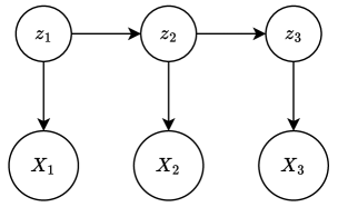
Figure 19. A simple Hidden Markov Model where hidden states $\mathbf{z}$ generate observations $\mathbf{X}$.

The sequence of hidden states $\mathbf{z_{1},z_{2},\dots,z_{n}}$ generates the corresponding sequence of observations $\mathbf{X_{1},X_{2},\dots,X_{n}}$. The model starts with an initial hidden state $\mathbf{z_{1}}$, and then the hidden state at each time step is determined by the transition probabilities $\mathbf{P(z_{i}\mid z_{i-1})}$, while the corresponding observation $\mathbf{X_{i}}$ is generated based on the emission probabilities $\mathbf{P(X_{i}\mid z_{i})}$.

Parameter Estimation The parameters of an HMM (transition probabilities, emission probabilities, and initial state probabilities) are typically estimated using the Expectation-Maximization (EM) algorithm (Dempster et al., 1977), specifically the Baum-Welch algorithm (Baum et al., 1970).

1) E-step: In this step, we estimate the posterior probabilities of the hidden states given the observations using the Forward-Backward algorithm:

$$\mathbf{\gamma_{ik}=\frac{P(z_{i}=k\mid X)}{\sum_{j}P(z_{i}=j\mid X)}}.$$

This represents the probability that the hidden state at time $i$ is $k$ given the observations.

2) M-step: In this step, we update the transition probabilities, emission probabilities, and initial probabilities based on the expected values computed in the E-step:

$$\mathbf{P(z_{i}=k\mid z_{i-1}=j)=\frac{\sum_{i=1}^{n}\gamma_{i-1,j}P(z_{i}=k\mid z_{i-1}=j)}{\sum_{i=1}^{n}\gamma_{i-1,j}}}.$$

Once the parameters of the HMM are estimated using the EM algorithm, synthetic data can be generated by sampling from the learned model. The synthetic data sequence $\mathbf{X_{\text{syn}}=\{X^{\prime}_{1},X^{\prime}_{2},X^{\prime}_{3}\}}$ is generated as follows:

1. Sample the initial state $\mathbf{z_{1}}$ from $\mathbf{P(z_{1})}$.

2. For each time step $i$:

   • Sample $\mathbf{z_{i}}$ from $\mathbf{P(z_{i}\mid z_{i-1})}$.

   • Sample $\mathbf{X^{\prime}_{i}}$ from $\mathbf{P(X^{\prime}_{i}\mid z_{i})}$.

This process leverages the estimated parameters from the EM algorithm to ensure that the generated sequences maintain the statistical dependencies of the original data. Suppose we want to generate synthetic data for a speech recognition task. The hidden states represent phonemes, and the observations are audio feature vectors. By estimating the parameters of the HMM, we can generate realistic synthetic speech sequences that follow the learned probabilistic patterns.

Hidden Markov Models (HMMs) are widely used for modeling sequential data, with applications in speech recognition, natural language processing, and time-series analysis. Using the EM algorithm, we can estimate HMM parameters and generate synthetic data sequences $\mathbf{X_{\text{syn}}}$ that closely resemble real-world sequences.

B.3. Data Types

Table B.6. Types of Data in Synthetic Data

Data Type	Example	Common Techniques
Tabular	Credit risk datasets (Kaggle, nd), census data, electronic health records.	FCT-GAN (Zhao et al., 2022),CTGAN (Xu et al., 2019), EHR-Safe (Yoon et al., 2023).
Images	Medical imaging, facial recognition, satellite imagery.	MedGAN (Armanious et al., 2020), SatGAN (Shah et al., 2021).
Time Series	Stock prices, sensor readings, physiological signals (EEG, ECG).	Fin-Gan (Vuletić et al., 2024), SeqGAN(Yu et al., 2017),(Delaney et al., 2019).
Text	Chatbot responses, document generation, structured reports.	GPT (Radford, 2018), BERT (Devlin, 2018),T5 (Raffel et al., 2020).
Graphs	Social networks.	Social GAN (Gupta et al., 2018).
Audio	Speech synthesis, music generation, environmental sounds.	Tacotron (Wang et al., 2017), MuseGan (Dong et al., 2018), WaveGAN (Van Den Oord et al., 2016).
Video	Video Synthesis, Text-to-video	VideoMAE (Tong et al., 2022), (Wang et al., 2018), (Li et al., 2018).
3D Data	Autonomous driving, medical 3D scans, virtual environments.	SAD-GAN (Ghosh et al., 2016), (Kwon et al., 2019), NeRF (Mildenhall et al., 2021).

Appendix C Taxonomy

Table C.7. Overview of Synthetic Data Generation Methods for Tabular Data. This table presents a comprehensive overview of various synthetic data generation models for tabular data, elucidating how each method addresses critical aspects, including feature dependencies (FDs), preservation of statistical properties (PSPs), conditioning on specific attributes (CSAs), and privacy preservation (PP). The methods are categorized into Traditional and Modern approaches including Autoregressive models (AR). Traditional methods include techniques like Autoencoders (AEs), Variational Autoencoders (VAEs), SMOTE, Gaussian Mixture Models (GMMs), Markov Chains, Bayesian Networks, and other statistical models, which rely on probabilistic or heuristic methods for data generation and feature modeling. The symbols in the table represent the following: a single tick mark ($\checkmark$) signifies that the method provides an enhanced or specialized treatment, such as more robust handling of that characteristic. An ($\times$) signifies that the method does not explicitly address the characteristic.

—p0.2—¿ p0.05—¿p0.05—¿p0.05—¿p0.05—¿p0.1—¿p0.05—¿p0.08—¿ p0.05—¿p0.06— []2-1Approaches Characteristics   Methods and Models  
[fill=tabheadcolor]1-1 FDs PSPs CSAs PP Traditional GANs Diffusion AR Masked
Xu et al., 2019 (Xu et al., 2019) $\checkmark$ $\times$ $\checkmark$
Zhao et al., 2022 (Zhao et al., 2022) $\checkmark$ $\times$ $\checkmark$
Zhao et al., 2021 (Zhao et al., 2021) $\checkmark$ $\checkmark$ $\checkmark$ $\times$ $\checkmark$
Jordon et al., 2018 (Jordon et al., 2018) $\checkmark$ $\checkmark$
Lee et al., 2021 (Lee et al., 2021) $\times$ $\checkmark$
Xu et al., 2019 (Xu et al., 2019) $\times$ $\checkmark$
Rajabi et al., 2022 (Rajabi and Garibay, 2022) $\times$ $\checkmark$
Park et al., 2018 (Park et al., 2018) $\times$ $\checkmark$
Xu et al., 2019 (Xu et al., 2019) $\checkmark$ $\checkmark$ $\times$ $\times$ $\checkmark$
Han et al., 2019 (Han et al., 2005) $\times$ $\times$ $\times$ $\times$ $\checkmark$
He et al., 2019 (He et al., 2008) $\times$ $\times$ $\times$ $\times$ $\checkmark$
Zhang et al., 2017 (Zhang et al., 2017) $\checkmark$ $\checkmark$ $\checkmark$
Ping et al., 2017 (Ping et al., 2017) $\checkmark$ $\checkmark$ $\checkmark$
Kotelnikov et al., 2023 (Kotelnikov et al., 2023) $\checkmark$ $\times$ $\checkmark$ $\checkmark$

Kim et. al,2022 (Kim et al., 2022) $\checkmark$ $\checkmark$ $\times$ $\times$ $\checkmark$
Zhang et. al,2023 (Zhang et al., 2023) $\checkmark$ $\checkmark$ $\times$ $\checkmark$ $\checkmark$ $\checkmark$
Jolicoeur et. al,2024 (Jolicoeur-Martineau et al., 2024) $\times$ $\checkmark$
Huang et al., 2020 (Huang et al., 2020) $\checkmark$ $\times$ $\checkmark$
Gulati et al., 2023 (Gulati and Roysdon, 2023) $\checkmark$ $\times$ $\checkmark$ $\checkmark$
Borisov et al., 2022 (Borisov et al., 2022) $\times$ $\checkmark$

Kamthe et al., 2021 (Kamthe et al., 2021) $\checkmark$ $\checkmark$ $\times$ $\checkmark$
Kate et al., 2022 (Kate et al., 2022) $\times$ $\times$ $\times$ $\times$ $\checkmark$
Choi et al., 2017 (Choi et al., 2017) $\checkmark$ $\times$ $\checkmark$
Che et al., 2017 (Che et al., 2017) $\checkmark$ $\checkmark$
Yoon et al., 2023 (Yoon et al., 2023) $\checkmark$ $\checkmark$
Abay et al., 2022 (Abay et al., 2019) $\times$ $\times$ $\checkmark$ $\checkmark$ $\checkmark$
Acs et al., 2018 (Acs et al., 2018) $\times$ $\times$ $\checkmark$ $\checkmark$ $\checkmark$
Fang et al., 2022 (Fang et al., 2022) $\checkmark$ $\checkmark$
Aviñó et. al,2018 (Aviñó et al., 2018) $\times$ $\times$ $\checkmark$

Appendix D Evaluation: Metrics for the existing models

To summarize the evaluation metrics used in prior literature, it is crucial to assess synthetic data generation models across key aspects such as data similarity, privacy preservation, and machine learning utility. These evaluations typically focus on categories like feature dependency, statistical similarity, and privacy preservation, alongside performance on machine learning tasks such as classification and regression. The metrics employed vary across models, reflecting their specific design objectives and intended use cases.

Feature Dependency

is one of the key considerations when evaluating synthetic data. It is essential to determine how well the synthetic data preserves the relationships between features found in the original dataset. Feature dependency preservation is evaluated by comparing the pairwise correlations between the features in the synthetic data and the original data. This is typically done using the Pearson correlation coefficient for continuous features, the uncertainty coefficient for categorical features, and the correlation ratio for mixed-type data. The Pearson correlation between two continuous variables $\mathbf{x_{1}}$ and $\mathbf{x_{2}}$ is calculated as:

(16) $$r_{\mathbf{x_{1},x_{2}}}=\frac{\mathbf{\text{Cov}(x_{1},x_{2})}}{\mathbf{\sigma_{x_{1}}\sigma_{x_{2}}}},$$

where $\mathbf{\text{Cov}(x_{1},x_{2})}$ represents the covariance between $\mathbf{x_{1}}$ and $\mathbf{x_{2}}$, and $\sigma_{\mathbf{x_{1}}}$ and $\sigma_{\mathbf{x_{2}}}$ are the standard deviations of $\mathbf{x_{1}}$ and $\mathbf{x_{2}}$, respectively. The closer this value is to 1 or -1, the stronger the linear relationship between the two variables.

Statistical Similarity

is another important evaluation criterion in synthetic data generation. Various divergence measures quantify the difference between the distributions of real and synthetic data. Two key metrics for this evaluation are the Jensen-Shannon Divergence (JSD) (Lin, 1991) and the Wasserstein Distance (WD) (Ramdas et al., 2017). The JSD is used to measure the difference between the probability distributions of categorical features in real and synthetic data. The JSD for two probability distributions $P$ and $Q$ is given by:

(17) $$\text{JSD}(P,Q)=\frac{1}{2}\left(D_{\text{KL}}(P\parallel M)+D_{\text{KL}}(Q\parallel M)\right),$$

where $M=\frac{1}{2}(P+Q)$, and $D_{\text{KL}}$ is the Kullback-Leibler divergence.

The Wasserstein Distance is often used for continuous variables, as it is numerically more stable than the JSD, especially when there is no overlap between the synthetic and original data distributions. The Wasserstein Distance between two distributions $P$ and $Q$ is defined as:

(18) $$W(P,Q)=\inf_{\gamma\in\Gamma(P,Q)}\mathbb{E}_{(x,y)\sim\gamma}\left[\|x-y\|\right],$$

where $\Gamma(P,Q)$ is the set of all possible couplings of $P$ and $Q$, and $\|x-y\|$ represents the distance between two points in the sample space.

Privacy Preservation

can be evaluated using metrics such as the privacy loss and the privacy-utility trade-off. Differential privacy ensures that an individual’s contribution to the dataset remains indistinguishable, even if the synthetic data is used in downstream tasks (Dwork et al., 2016). Formally, a mechanism $M$ satisfies $\epsilon$-differential privacy if, for all neighboring datasets $D_{1}$ and $D_{2}$ (differing by at most one individual), and for all outputs $S\subseteq\text{Range}(M)$:

$$\frac{\Pr[M(D_{1})\in S]}{\Pr[M(D_{2})\in S]}\leq e^{\epsilon}.$$

Here, $\epsilon$ is the privacy loss, which quantifies the strength of the privacy guarantee (Dwork et al., 2014). Lower values of $\epsilon$ correspond to stronger privacy, as they limit the influence of any single individual on the output. The privacy loss is typically controlled by adding noise to the model’s outputs using mechanisms such as the Laplace noise or Gaussian noise (Dwork et al., 2016). For example, the Laplace mechanism adds noise drawn from the Laplace distribution:

$$M(D)=f(D)+\text{Laplace}\left(0,\frac{\Delta f}{\epsilon}\right),$$

where $\Delta f$ is the sensitivity of the query $f$, defined as the maximum change in the output when one individual is added or removed from the dataset (Dwork et al., 2014). Similarly, the Gaussian mechanism adds noise drawn from a Gaussian distribution:

$$M(D)=f(D)+\mathcal{N}\left(0,\sigma^{2}\right),$$

where $\sigma$ is scaled based on $\epsilon$ and the sensitivity $\Delta f$ (Dwork et al., 2014). The privacy budget $\epsilon$ represents the total allowable privacy loss across multiple queries or iterations (Dwork et al., 2016). A smaller $\epsilon$ provides stronger privacy guarantees but may reduce the utility of the output due to increased noise. This trade-off is critical in applications where both privacy and data usefulness are important. PATE-GAN enforces strict privacy constraints while maintaining a high level of utility, making it a suitable model for privacy-sensitive applications. To evaluate utility, metrics such as the Area Under the Receiver Operating Characteristics Curve (AUROC) and the Area Under the Precision-Recall Curve (AUPRC) are often used (Jordon et al., 2018). AUROC measures how well a model distinguishes between classes, while AUPRC is particularly useful for evaluating performance on imbalanced datasets (Jordon et al., 2018). These metrics help quantify the effectiveness of synthetic data in training privacy-preserving models while maintaining high utility.

Machine Learning Utility

measures the effectiveness of synthetic data for downstream tasks like classification and regression. ML utility is often evaluated by training machine learning classifiers or regressors on the synthetic data and comparing their performance to that of models trained on the original data. Metrics such as accuracy, F1-score, and AUC are used for classification, while for regression tasks, mean absolute percentage error (MAPE), explained variance score (EVS), and R² score are used. These metrics help determine whether the synthetic data retains the predictive power of the original data. For example, the F1-score, which is a harmonic mean of precision and recall, is calculated as:

(19) $$F_{1}=2\cdot\frac{\text{precision}\cdot\text{recall}}{\text{precision}+\text{recall}},$$

where precision and recall are defined as:

(20) $$\text{precision}=\frac{TP}{TP+FP},\quad\text{recall}=\frac{TP}{TP+FN},$$

with $TP$, $FP$, and $FN$ representing the true positives, false positives, and false negatives, respectively. The AUC measures the area under the ROC curve, which plots the true positive rate against the false positive rate at various threshold settings. In regression tasks, the R² score quantifies the proportion of variance in the target variable that is predictable from the features:

(21) $$R^{2}=1-\frac{\sum_{i=1}^{n}(y_{i}-\hat{y}_{i})^{2}}{\sum_{i=1}^{n}(y_{i}-\bar{y})^{2}},$$

where $y_{i}$ represents the true values, $\hat{y}_{i}$ are the predicted values, and $\bar{y}$ is the mean of the true values. Similarly, MAPE is defined as:

(22) $$MAPE=\frac{1}{n}\sum_{i=1}^{n}\left|\frac{y_{i}-\hat{y}_{i}}{y_{i}}\right|\times 100\%,$$

which calculates the average absolute percentage error between the predicted and true values.

Overall, these findings underscore the importance of selecting the right model based on the specific requirements of the task, whether that be for better privacy preservation, statistical similarity, or machine learning utility, as no one model outperforms others across all categories. Table D.8 provides the summary of the evaluation metrics for the models discussed.

Table D.8. Summary of Evaluation Metrics for Synthetic Data Generation Models

Metric	Method
Feature Dependency	Pearson Correlation (Continuous), Uncertainty Coefficient (Categorical), Correlation Ratio (Mixed)
Statistical Similarity	Jensen-Shannon Divergence (JSD), Wasserstein Distance (WD), Area Under the Receiver Operating Characteristics Curv (AUROC), Area Under the Precision-Recall Curve (AUPRC).
Privacy Preservation	Model Inversion attacks, Membership-inference attacks, Privacy Loss ($\epsilon$), Privacy-Utility Trade-off ($\epsilon$ vs. AUROC/AUPRC)
Machine Learning Utility	Accuracy, F1-score, AUC, MAPE, EVS, R² (Regression),AUROC, AUPRC.

References

- (1)
- Abay et al. (2019) Nazmiye Ceren Abay, Yan Zhou, Murat Kantarcioglu, Bhavani Thuraisingham, and Latanya Sweeney. 2019. Privacy preserving synthetic data release using deep learning. In Machine Learning and Knowledge Discovery in Databases: European Conference, ECML PKDD 2018, Dublin, Ireland, September 10–14, 2018, Proceedings, Part I 18. Springer, 510–526.
- Acs et al. (2018) Gergely Acs, Luca Melis, Claude Castelluccia, and Emiliano De Cristofaro. 2018. Differentially private mixture of generative neural networks. IEEE Transactions on Knowledge and Data Engineering 31, 6 (2018), 1109–1121.
- Amplitude (2024) Amplitude. 2024. What Is Data Democratization? Definition and Principles. https://www.amplitude.com/blog/data-democratization
- Annamalai et al. (2024) Meenatchi Sundaram Muthu Selva Annamalai, Andrea Gadotti, and Luc Rocher. 2024. A linear reconstruction approach for attribute inference attacks against synthetic data. In 33rd USENIX Security Symposium (USENIX Security 24). 2351–2368.
- Arjovsky et al. (2017) Martin Arjovsky, Soumith Chintala, and Léon Bottou. 2017. Wasserstein generative adversarial networks. In International conference on machine learning. PMLR, 214–223.
- Armanious et al. (2020) Karim Armanious, Chenming Jiang, Marc Fischer, Thomas Küstner, Tobias Hepp, Konstantin Nikolaou, Sergios Gatidis, and Bin Yang. 2020. MedGAN: Medical image translation using GANs. Computerized medical imaging and graphics 79 (2020), 101684.
- Arthur (2013) Lisa Arthur. 2013. Big data marketing: engage your customers more effectively and drive value. John Wiley & Sons.
- Assefa et al. (2020) Samuel A Assefa, Danial Dervovic, Mahmoud Mahfouz, Robert E Tillman, Prashant Reddy, and Manuela Veloso. 2020. Generating synthetic data in finance: opportunities, challenges and pitfalls. In Proceedings of the First ACM International Conference on AI in Finance. 1–8.
- Aviñó et al. (2018) Laura Aviñó, Matteo Ruffini, and Ricard Gavaldà. 2018. Generating synthetic but plausible healthcare record datasets. arXiv preprint arXiv:1807.01514 (2018).
- Babbar and Schölkopf (2019) Rohit Babbar and Bernhard Schölkopf. 2019. Data scarcity, robustness and extreme multi-label classification. Machine Learning 108, 8 (2019), 1329–1351.
- Bauer et al. (2024) André Bauer, Simon Trapp, Michael Stenger, Robert Leppich, Samuel Kounev, Mark Leznik, Kyle Chard, and Ian Foster. 2024. Comprehensive exploration of synthetic data generation: A survey. arXiv preprint arXiv:2401.02524 (2024).
- Baum et al. (1970) Leonard E Baum, Ted Petrie, George Soules, and Norman Weiss. 1970. A maximization technique occurring in the statistical analysis of probabilistic functions of Markov chains. The annals of mathematical statistics 41, 1 (1970), 164–171.
- Becker and Kohavi (1996) Barry Becker and Ronny Kohavi. 1996. Adult. UCI Machine Learning Repository. DOI: https://doi.org/10.24432/C5XW20.
- Bindschaedler et al. (2017) Vincent Bindschaedler, Reza Shokri, and Carl A Gunter. 2017. Plausible deniability for privacy-preserving data synthesis. arXiv preprint arXiv:1708.07975 (2017).
- Bishop and Nasrabadi (2006) Christopher M Bishop and Nasser M Nasrabadi. 2006. Pattern recognition and machine learning. Vol. 4. Springer.
- Borisov et al. (2022) Vadim Borisov, Kathrin Seßler, Tobias Leemann, Martin Pawelczyk, and Gjergji Kasneci. 2022. Language models are realistic tabular data generators. arXiv preprint arXiv:2210.06280 (2022).
- Box et al. (2015) George EP Box, Gwilym M Jenkins, Gregory C Reinsel, and Greta M Ljung. 2015. Time series analysis: forecasting and control. John Wiley & Sons.
- Chang et al. (2022) Huiwen Chang, Han Zhang, Lu Jiang, Ce Liu, and William T Freeman. 2022. Maskgit: Masked generative image transformer. In Proceedings of the IEEE/CVF conference on computer vision and pattern recognition. 11315–11325.
- Chawla et al. (2002) Nitesh V Chawla, Kevin W Bowyer, Louis O Hall, and Wayne P Kegelmeyer. 2002. SMOTE: Synthetic Minority Over-sampling Technique. Journal of Artificial Intelligence Research 16 (2002), 321–357.
- Che et al. (2017) Zhengping Che, Yu Cheng, Shuangfei Zhai, Zhaonan Sun, and Yan Liu. 2017. Boosting deep learning risk prediction with generative adversarial networks for electronic health records. In 2017 IEEE International Conference on Data Mining (ICDM). IEEE, 787–792.
- Choi et al. (2017) Edward Choi, Siddharth Biswal, Bradley Malin, Jon Duke, Walter F Stewart, and Jimeng Sun. 2017. Generating multi-label discrete patient records using generative adversarial networks. In Machine learning for healthcare conference. PMLR, 286–305.
- Chouldechova and Roth (2018) Alexandra Chouldechova and Aaron Roth. 2018. The frontiers of fairness in machine learning. arXiv preprint arXiv:1810.08810 (2018).
- Clim et al. (2019) Antonio Clim, Razvan Daniel Zota, and Grigore Tinica. 2019. Big Data in home healthcare: A new frontier in personalized medicine. Medical emergency services and prediction of hypertension risks. International Journal of Healthcare Management 12, 3 (2019), 241–249.
- Council (2023) Forbes Technology Council. 2023. The New Era Of Big Data. (2023). https://www.forbes.com/councils/forbestechcouncil/2023/05/24/the-new-era-of-big-data/ Accessed: 2025-01-18.
- Dal Pozzolo et al. (2017) Andrea Dal Pozzolo, Giacomo Boracchi, Olivier Caelen, Cesare Alippi, and Gianluca Bontempi. 2017. Credit card fraud detection: a realistic modeling and a novel learning strategy. IEEE transactions on neural networks and learning systems 29, 8 (2017), 3784–3797.
- Delaney et al. (2019) Anne Marie Delaney, Eoin Brophy, and Tomas E Ward. 2019. Synthesis of realistic ECG using generative adversarial networks. arXiv preprint arXiv:1909.09150 (2019).
- Dempster et al. (1977) Arthur P Dempster, Nan M Laird, and Donald B Rubin. 1977. Maximum likelihood from incomplete data via the EM algorithm. Journal of the royal statistical society: series B (methodological) 39, 1 (1977), 1–22.
- Devlin (2018) Jacob Devlin. 2018. Bert: Pre-training of deep bidirectional transformers for language understanding. arXiv preprint arXiv:1810.04805 (2018).
- Dhariwal and Nichol (2021) Prafulla Dhariwal and Alexander Nichol. 2021. Diffusion models beat gans on image synthesis. Advances in neural information processing systems 34 (2021), 8780–8794.
- Dong et al. (2018) Hao-Wen Dong, Wen-Yi Hsiao, Li-Chia Yang, and Yi-Hsuan Yang. 2018. Musegan: Multi-track sequential generative adversarial networks for symbolic music generation and accompaniment. In Proceedings of the AAAI conference on artificial intelligence, Vol. 32.
- Dosovitskiy et al. (2017) Alexey Dosovitskiy, German Ros, Felipe Codevilla, Antonio Lopez, and Vladlen Koltun. 2017. CARLA: An open urban driving simulator. In Conference on robot learning. PMLR, 1–16.
- Douzas and Bacao (2019) Georgios Douzas and Fernando Bacao. 2019. Geometric SMOTE a geometrically enhanced drop-in replacement for SMOTE. Information sciences 501 (2019), 118–135.
- Durkan et al. (2019) Conor Durkan, Artur Bekasov, Iain Murray, and George Papamakarios. 2019. Neural spline flows. Advances in neural information processing systems 32 (2019).
- Dwork (2006) Cynthia Dwork. 2006. Differential privacy. In International colloquium on automata, languages, and programming. Springer, 1–12.
- Dwork et al. (2016) Cynthia Dwork, Frank McSherry, Kobbi Nissim, and Adam Smith. 2016. Calibrating noise to sensitivity in private data analysis. Journal of Privacy and Confidentiality 7, 3 (2016), 17–51.
- Dwork et al. (2014) Cynthia Dwork, Aaron Roth, et al. 2014. The algorithmic foundations of differential privacy. Foundations and Trends® in Theoretical Computer Science 9, 3–4 (2014), 211–407.
- European Union (2016) European Union. 2016. General Data Protection Regulation. L119 pages. https://gdpr-info.eu Retrieved from https://gdpr-info.eu.
- Fang et al. (2022) Mei Ling Fang, Devendra Singh Dhami, and Kristian Kersting. 2022. Dp-ctgan: Differentially private medical data generation using ctgans. In International Conference on Artificial Intelligence in Medicine. Springer, 178–188.
- Figueira and Vaz (2022) Alvaro Figueira and Bruno Vaz. 2022. Survey on synthetic data generation, evaluation methods and GANs. Mathematics 10, 15 (2022), 2733.
- Flores et al. (2022) Vaneza Flores, Stella Heras, and Vicente Julian. 2022. Comparison of predictive models with balanced classes using the SMOTE method for the forecast of student dropout in higher education. Electronics 11, 3 (2022), 457.
- Fredrikson et al. (2014) Matthew Fredrikson, Eric Lantz, Somesh Jha, Simon Lin, David Page, and Thomas Ristenpart. 2014. Privacy in pharmacogenetics: An End-to-End case study of personalized warfarin dosing. In 23rd USENIX security symposium (USENIX Security 14). 17–32.
- Ghatak and Sakurai (2022) Debolina Ghatak and Kouichi Sakurai. 2022. A survey on privacy preserving synthetic data generation and a discussion on a privacy-utility trade-off problem. In International Conference on Science of Cyber Security. Springer, 167–180.
- Ghosh et al. (2016) Arna Ghosh, Biswarup Bhattacharya, and Somnath Basu Roy Chowdhury. 2016. Sad-gan: Synthetic autonomous driving using generative adversarial networks. arXiv preprint arXiv:1611.08788 (2016).
- Goan and Fookes (2020) Ethan Goan and Clinton Fookes. 2020. Bayesian Neural Networks: An Introduction and Survey. arXiv preprint arXiv:2006.12024 (2020).
- Goodfellow et al. (2014) Ian Goodfellow, Jean Pouget-Abadie, Mehdi Mirza, Bing Xu, David Warde-Farley, Sherjil Ozair, Aaron Courville, and Yoshua Bengio. 2014. Generative adversarial nets. Advances in neural information processing systems 27 (2014).
- Gretel.ai (2023) Gretel.ai. 2023. What is synthetic data? https://gretel.ai/technical-glossary/what-is-synthetic-data Accessed: 2025-01-22.
- Guan et al. (2024) Vincent Guan, Florent Guépin, Ana-Maria Cretu, and Yves-Alexandre de Montjoye. 2024. A zero auxiliary knowledge membership inference attack on aggregate location data. arXiv preprint arXiv:2406.18671 (2024).
- Gulati and Roysdon (2023) Manbir Gulati and Paul Roysdon. 2023. TabMT: Generating tabular data with masked transformers. Advances in Neural Information Processing Systems 36 (2023), 46245–46254.
- Gupta et al. (2018) Agrim Gupta, Justin Johnson, Li Fei-Fei, Silvio Savarese, and Alexandre Alahi. 2018. Social gan: Socially acceptable trajectories with generative adversarial networks. In Proceedings of the IEEE conference on computer vision and pattern recognition. 2255–2264.
- Han et al. (2005) Hui Han, Wen-Yuan Wang, and Bing-Huan Mao. 2005. Borderline-SMOTE: a new over-sampling method in imbalanced data sets learning. In International conference on intelligent computing. Springer, 878–887.
- He et al. (2008) Haibo He, Yang Bai, Edwardo A Garcia, and Shutao Li. 2008. ADASYN: Adaptive synthetic sampling approach for imbalanced learning. In 2008 IEEE international joint conference on neural networks (IEEE world congress on computational intelligence). Ieee, 1322–1328.
- He and Garcia (2009) Haibo He and Edward A Garcia. 2009. Learning from imbalanced data. IEEE Transactions on Knowledge and Data Engineering 21, 9 (2009), 1263–1284.
- Hernandez et al. (2022) Mikel Hernandez, Gorka Epelde, Ane Alberdi, Rodrigo Cilla, and Debbie Rankin. 2022. Synthetic data generation for tabular health records: A systematic review. Neurocomputing 493 (2022), 28–45.
- Ho et al. (2020) Jonathan Ho, Ajay Jain, and Pieter Abbeel. 2020. Denoising diffusion probabilistic models. Advances in neural information processing systems 33 (2020), 6840–6851.
- Hoogeboom et al. (2021a) Emiel Hoogeboom, Alexey A Gritsenko, Jasmijn Bastings, Ben Poole, Rianne van den Berg, and Tim Salimans. 2021a. Autoregressive diffusion models. arXiv preprint arXiv:2110.02037 (2021).
- Hoogeboom et al. (2021b) Emiel Hoogeboom, Didrik Nielsen, Priyank Jaini, Patrick Forré, and Max Welling. 2021b. Argmax flows and multinomial diffusion: Learning categorical distributions. Advances in Neural Information Processing Systems 34 (2021), 12454–12465.
- Hu et al. (2020) Mengxiao Hu, Jinlong Li, Maolin Hu, and Tao Hu. 2020. Hierarchical modes exploring in generative adversarial networks. In Proceedings of the AAAI Conference on Artificial Intelligence, Vol. 34. 10981–10988.
- Huang et al. (2020) Xin Huang, Ashish Khetan, Milan Cvitkovic, and Zohar Karnin. 2020. Tabtransformer: Tabular data modeling using contextual embeddings. arXiv preprint arXiv:2012.06678 (2020).
- Jolicoeur-Martineau et al. (2024) Alexia Jolicoeur-Martineau, Kilian Fatras, and Tal Kachman. 2024. Generating and imputing tabular data via diffusion and flow-based gradient-boosted trees. In International Conference on Artificial Intelligence and Statistics. PMLR, 1288–1296.
- Jordon et al. (2018) James Jordon, Jinsung Yoon, and Mihaela Van Der Schaar. 2018. PATE-GAN: Generating synthetic data with differential privacy guarantees. In International conference on learning representations.
- Kaggle (nd) Kaggle. n.d.. Credit Risk Dataset. https://www.kaggle.com/datasets/laotse/credit-risk-dataset Accessed: 2025-01-28.
- Kamthe et al. (2021) Sanket Kamthe, Samuel Assefa, and Marc Deisenroth. 2021. Copula flows for synthetic data generation. arXiv preprint arXiv:2101.00598 (2021).
- Karras et al. (2019) Tero Karras, Samuli Laine, and Timo Aila. 2019. A style-based generator architecture for generative adversarial networks. In Proceedings of the IEEE/CVF conference on computer vision and pattern recognition. 4401–4410.
- Kate et al. (2022) Prateek Kate, Vadlamani Ravi, and Akhilesh Gangwar. 2022. Fingan: Generative adversarial network for analytical customer relationship management in banking and insurance. arXiv preprint arXiv:2201.11486 (2022).
- Kim et al. (2022) Jayoung Kim, Chaejeong Lee, and Noseong Park. 2022. Stasy: Score-based tabular data synthesis. arXiv preprint arXiv:2210.04018 (2022).
- Kingma and Welling (2013) Diederik P Kingma and Max Welling. 2013. Auto-encoding variational bayes. arXiv preprint arXiv:1312.6114 (2013).
- Kotelnikov et al. (2023) Akim Kotelnikov, Dmitry Baranchuk, Ivan Rubachev, and Artem Babenko. 2023. Tabddpm: Modelling tabular data with diffusion models. In International Conference on Machine Learning. PMLR, 17564–17579.
- Kwon et al. (2019) Gihyun Kwon, Chihye Han, and Dae-shik Kim. 2019. Generation of 3D brain MRI using auto-encoding generative adversarial networks. In International Conference on Medical Image Computing and Computer-Assisted Intervention. Springer, 118–126.
- Lee et al. (2021) Jaehoon Lee, Jihyeon Hyeong, Jinsung Jeon, Noseong Park, and Jihoon Cho. 2021. Invertible tabular GANs: Killing two birds with one stone for tabular data synthesis. Advances in Neural Information Processing Systems 34 (2021), 4263–4273.
- Li et al. (2018) Yitong Li, Martin Min, Dinghan Shen, David Carlson, and Lawrence Carin. 2018. Video generation from text. In Proceedings of the AAAI conference on artificial intelligence, Vol. 32.
- Li et al. (2020) Zongyi Li, Nikola Kovachki, Kamyar Azizzadenesheli, Burigede Liu, Kaushik Bhattacharya, Andrew Stuart, and Anima Anandkumar. 2020. Fourier neural operator for parametric partial differential equations. arXiv preprint arXiv:2010.08895 (2020).
- Lin (1991) Jianhua Lin. 1991. Divergence measures based on the Shannon entropy. IEEE Transactions on Information theory 37, 1 (1991), 145–151.
- Lu et al. (2023) Yingzhou Lu, Minjie Shen, Huazheng Wang, Xiao Wang, Capucine van Rechem, and Wenqi Wei. 2023. Machine learning for synthetic data generation: a review. arXiv preprint arXiv:2302.04062 (2023).
- Ma et al. (2018) Chao Ma, Sebastian Tschiatschek, Konstantina Palla, José Miguel Hernández-Lobato, Sebastian Nowozin, and Cheng Zhang. 2018. Eddi: Efficient dynamic discovery of high-value information with partial vae. arXiv preprint arXiv:1809.11142 (2018).
- Mildenhall et al. (2021) Ben Mildenhall, Pratul P Srinivasan, Matthew Tancik, Jonathan T Barron, Ravi Ramamoorthi, and Ren Ng. 2021. Nerf: Representing scenes as neural radiance fields for view synthesis. Commun. ACM 65, 1 (2021), 99–106.
- Nelsen (2006) Roger B Nelsen. 2006. An introduction to copulas. Springer.
- Nichol and Dhariwal (2021) Alexander Quinn Nichol and Prafulla Dhariwal. 2021. Improved denoising diffusion probabilistic models. In International conference on machine learning. PMLR, 8162–8171.
- of Health and Services (1996) U.S. Department of Health and Human Services. 1996. Health Insurance Portability and Accountability Act of 1996 (HIPAA). https://www.hhs.gov/hipaa
- Papernot et al. (2016) Nicolas Papernot, Martín Abadi, Ulfar Erlingsson, Ian Goodfellow, and Kunal Talwar. 2016. Semi-supervised knowledge transfer for deep learning from private training data. arXiv preprint arXiv:1610.05755 (2016).
- Park et al. (2018) Noseong Park, Mahmoud Mohammadi, Kshitij Gorde, Sushil Jajodia, Hongkyu Park, and Youngmin Kim. 2018. Data synthesis based on generative adversarial networks. arXiv preprint arXiv:1806.03384 (2018).
- Patki et al. (2016) Neha Patki, Roy Wedge, and Kalyan Veeramachaneni. 2016. The synthetic data vault. In 2016 IEEE international conference on data science and advanced analytics (DSAA). IEEE, 399–410.
- Pearl (2014) Judea Pearl. 2014. Probabilistic reasoning in intelligent systems: networks of plausible inference. Elsevier.
- Ping et al. (2017) Haoyue Ping, Julia Stoyanovich, and Bill Howe. 2017. Datasynthesizer: Privacy-preserving synthetic datasets. In Proceedings of the 29th International Conference on Scientific and Statistical Database Management. 1–5.
- Rabiner (1989) Lawrence R Rabiner. 1989. A tutorial on hidden Markov models and selected applications in speech recognition. Proc. IEEE 77, 2 (1989), 257–286.
- Radford (2018) Alec Radford. 2018. Improving language understanding by generative pre-training. (2018).
- Raffel et al. (2020) Colin Raffel, Noam Shazeer, Adam Roberts, Katherine Lee, Sharan Narang, Michael Matena, Yanqi Zhou, Wei Li, and Peter J Liu. 2020. Exploring the limits of transfer learning with a unified text-to-text transformer. Journal of machine learning research 21, 140 (2020), 1–67.
- Rahman et al. (2023) Md. Arafatur Rahman, Alireza Moayedikia, and Uffe Kock Wiil. 2023. Editorial: Data-driven technologies for future healthcare systems. Frontiers in Medical Technology 5 (2023), 1183687. doi:10.3389/fmedt.2023.1183687
- Rajabi and Garibay (2022) Amirarsalan Rajabi and Ozlem Ozmen Garibay. 2022. Tabfairgan: Fair tabular data generation with generative adversarial networks. Machine Learning and Knowledge Extraction 4, 2 (2022), 488–501.
- Ramdas et al. (2017) Aaditya Ramdas, Nicolás García Trillos, and Marco Cuturi. 2017. On wasserstein two-sample testing and related families of nonparametric tests. Entropy 19, 2 (2017), 47.
- Reynolds et al. (2009) Douglas A Reynolds et al. 2009. Gaussian mixture models. Encyclopedia of biometrics 741, 659-663 (2009).
- Scarselli et al. (2008) Franco Scarselli, Marco Gori, Ah Chung Tsoi, Markus Hagenbuchner, and Gabriele Monfardini. 2008. The graph neural network model. IEEE transactions on neural networks 20, 1 (2008), 61–80.
- Shah et al. (2021) Mitt Shah, Manish Gupta, and Priyank Thakkar. 2021. SatGAN: Satellite image generation using conditional adversarial networks. In 2021 International Conference on Communication information and Computing Technology (ICCICT). IEEE, 1–6.
- Song et al. (2020a) Jiaming Song, Chenlin Meng, and Stefano Ermon. 2020a. Denoising diffusion implicit models. arXiv preprint arXiv:2010.02502 (2020).
- Song et al. (2020b) Yang Song, Jascha Sohl-Dickstein, Diederik P Kingma, Abhishek Kumar, Stefano Ermon, and Ben Poole. 2020b. Score-based generative modeling through stochastic differential equations. arXiv preprint arXiv:2011.13456 (2020).
- Syntheticus.ai (2023) Syntheticus.ai. 2023. The benefits and limitations of generating synthetic data. https://syntheticus.ai/blog/the-benefits-and-limitations-of-generating-synthetic-data Accessed: 2025-01-22.
- Syntho.ai (2023) Syntho.ai. 2023. Synthetic data vs real data: which is the better choice? https://www.syntho.ai/synthetic-data-vs-real-data-which-is-the-better-choice/ Accessed: 2025-01-22.
- Tian et al. (2021) Xin Tian, Jing Selena He, and Meng Han. 2021. Data-driven approaches in FinTech: a survey. Information Discovery and Delivery 49, 2 (2021), 123–135.
- Tong et al. (2022) Zhan Tong, Yibing Song, Jue Wang, and Limin Wang. 2022. Videomae: Masked autoencoders are data-efficient learners for self-supervised video pre-training. Advances in neural information processing systems 35 (2022), 10078–10093.
- Van Den Oord et al. (2016) Aaron Van Den Oord, Sander Dieleman, Heiga Zen, Karen Simonyan, Oriol Vinyals, Alex Graves, Nal Kalchbrenner, Andrew Senior, Koray Kavukcuoglu, et al. 2016. Wavenet: A generative model for raw audio. arXiv preprint arXiv:1609.03499 12 (2016).
- Vaswani et al. (2017) Ashish Vaswani, Noam Shazeer, Niki Parmar, Jakob Uszkoreit, Llion Jones, Aidan N Gomez, Łukasz Kaiser, and Illia Polosukhin. 2017. Attention is all you need. Advances in neural information processing systems 30 (2017).
- Vishweswar Sastry et al. (2024) V. N. Vishweswar Sastry, D. R. Guruprasad Desai, Hemanth Kumar, and Manjushree M. 2024. Big Data Analytics in Finance: Predictive Modeling for Investment Strategies. European Economic Letters (EEL) 14, 3 (Aug. 2024), 572–581. https://eelet.org.uk/index.php/journal/article/view/1803
- Vuletić et al. (2024) Milena Vuletić, Felix Prenzel, and Mihai Cucuringu. 2024. Fin-gan: Forecasting and classifying financial time series via generative adversarial networks. Quantitative Finance 24, 2 (2024), 175–199.
- Wang et al. (2018) Ting-Chun Wang, Ming-Yu Liu, Jun-Yan Zhu, Guilin Liu, Andrew Tao, Jan Kautz, and Bryan Catanzaro. 2018. Video-to-video synthesis. arXiv preprint arXiv:1808.06601 (2018).
- Wang et al. (2017) Yuxuan Wang, RJ Skerry-Ryan, Daisy Stanton, Yonghui Wu, Ron J Weiss, Navdeep Jaitly, Zongheng Yang, Ying Xiao, Zhifeng Chen, Samy Bengio, et al. 2017. Tacotron: Towards end-to-end speech synthesis. arXiv preprint arXiv:1703.10135 (2017).
- Xia et al. (2024) Haochong Xia, Shuo Sun, Xinrun Wang, and Bo An. 2024. Market-gan: Adding control to financial market data generation with semantic context. In Proceedings of the AAAI Conference on Artificial Intelligence, Vol. 38. 15996–16004.
- Xu et al. (2019) Lei Xu, Maria Skoularidou, Alfredo Cuesta-Infante, and Kalyan Veeramachaneni. 2019. Modeling tabular data using conditional gan. Advances in neural information processing systems 32 (2019).
- Xu and Veeramachaneni (2018) Lei Xu and Kalyan Veeramachaneni. 2018. Synthesizing tabular data using generative adversarial networks. arXiv preprint arXiv:1811.11264 (2018).
- Yeom et al. (2018) Samuel Yeom, Irene Giacomelli, Matt Fredrikson, and Somesh Jha. 2018. Privacy risk in machine learning: Analyzing the connection to overfitting. In 2018 IEEE 31st computer security foundations symposium (CSF). IEEE, 268–282.
- Yoon et al. (2018) Jinsung Yoon, James Jordon, and Mihaela Schaar. 2018. Gain: Missing data imputation using generative adversarial nets. In International conference on machine learning. PMLR, 5689–5698.
- Yoon et al. (2023) Jinsung Yoon, Michel Mizrahi, Nahid Farhady Ghalaty, Thomas Jarvinen, Ashwin S Ravi, Peter Brune, Fanyu Kong, Dave Anderson, George Lee, Arie Meir, et al. 2023. EHR-Safe: generating high-fidelity and privacy-preserving synthetic electronic health records. NPJ Digital Medicine 6, 1 (2023), 141.
- Yoon et al. (2019) Jinsung Yoon, William Zame, and Mihaela van der Schaar. 2019. Time-Series Generative Adversarial Networks. Proceedings of the 36th International Conference on Machine Learning 97 (2019), 5614–5623.
- Yu et al. (2017) Lantao Yu, Weinan Zhang, Jun Wang, and Yong Yu. 2017. Seqgan: Sequence generative adversarial nets with policy gradient. In Proceedings of the AAAI conference on artificial intelligence, Vol. 31.
- Zemel et al. (2013) Rich Zemel, Yu Wu, Kevin Swersky, Toni Pitassi, and Cynthia Dwork. 2013. Learning fair representations. In International conference on machine learning. PMLR, 325–333.
- Zhang et al. (2023) Hengrui Zhang, Jiani Zhang, Balasubramaniam Srinivasan, Zhengyuan Shen, Xiao Qin, Christos Faloutsos, Huzefa Rangwala, and George Karypis. 2023. Mixed-type tabular data synthesis with score-based diffusion in latent space. arXiv preprint arXiv:2310.09656 (2023).
- Zhang et al. (2017) Jun Zhang, Graham Cormode, Cecilia M Procopiuc, Divesh Srivastava, and Xiaokui Xiao. 2017. Privbayes: Private data release via bayesian networks. ACM Transactions on Database Systems (TODS) 42, 4 (2017), 1–41.
- Zhang et al. (2020) Jun Zhang, Wei Wang, Feng Xia, Yu-Ru Lin, and Hanghang Tong. 2020. Data-driven computational social science: A survey. Big Data Research 21 (2020), 100145.
- Zhao and Zhang (2019) Wei Zhao and Li Zhang. 2019. Logistical challenges in data collection for machine learning. IEEE Transactions on Big Data 5, 3 (2019), 345–356.
- Zhao et al. (2022) Zilong Zhao, Robert Birke, and Lydia Y Chen. 2022. FCT-GAN: Enhancing Table Synthesis via Fourier Transform. arXiv preprint arXiv:2210.06239 (2022).
- Zhao et al. (2021) Zilong Zhao, Aditya Kunar, Robert Birke, and Lydia Y Chen. 2021. Ctab-gan: Effective table data synthesizing. In Asian Conference on Machine Learning. PMLR, 97–112.