Einstein Fields: A Neural Perspective to
Computational General Relativity

Abstract

We introduce Einstein Fields, a neural representation that is designed to compress computationally intensive four-dimensional numerical relativity simulations into compact implicit neural network weights. By modeling the metric, which is the core tensor field of general relativity, Einstein Fields enable the derivation of physical quantities via automatic differentiation. However, unlike conventional neural fields (e.g., signed distance, occupancy, or radiance fields), Einstein Fields are Neural Tensor Fields with the key difference that when encoding the spacetime geometry of general relativity into neural field representations, dynamics emerge naturally as a byproduct. Einstein Fields show remarkable potential, including continuum modeling of 4D spacetime, mesh-agnosticity, storage efficiency, derivative accuracy, and ease of use. We address these challenges across several canonical test beds of general relativity and release an open source JAX-based library, paving the way for more scalable and expressive approaches to numerical relativity. Code is made available at https://github.com/AndreiB137/EinFields.

1 Introduction

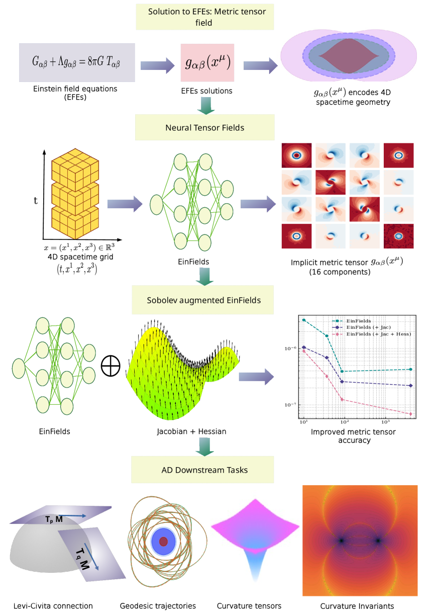
Figure 1: A conceptual overview of EinFields training and downstream pipeline. (i) Premise: The Einstein field equations (EFEs) in Equation (1) are highly non-linear partial differential equations defined on a 4D spacetime manifold, describing the geometric nature of gravitation. Their solutions define the metric tensor field $g_{\alpha\beta}(x^{\mu})$, which encodes the full spacetime geometry and serves as a tensorial generalization of the gravitational potential. In this work, we parametrize $g_{\alpha\beta}(x^{\mu})$ using a neural network. (ii) Training: The training is conducted on the metric tensor fields defined on a 4D spacetime grid. EinFields instead fit a continuous signal on these discrete representations, thus modeling 4D spacetime as a continuum, and returning the metric tensor field for a 4D spacetime query coordinate $p\equiv(t,x)\in\mathscr{M}$ at arbitrary resolution. (iii) Sobolev supervision: The reconstruction quality of the metric and its derivatives is improved by augmenting Sobolev losses, i.e., metric Jacobian (neighborhood structure) and Hessian (curvatures). (iv) Validation and downstream tasks: Sobolev improved EinFields’ AD-based derivatives enable accurate point-wise retrieval of differential geometric quantities, such as the Levi-Civita connection (covariant derivative), geodesics, curvature tensors, and their invariants.

General relativity (GR) is a foundational theory of modern physics that describes gravity as the curvature of spacetime caused by mass and energy. This curvature, along with angles, distances, geodesics, and causality, is encoded in the metric. At the heart of GR lie the Einstein field equations (EFEs), a set of coupled, tensor-valued, non-linear hyperbolic-elliptic partial differential equations (PDEs) that govern the metric behavior. EFEs are exceptionally complex, and exact analytical solutions exist only in idealized cases.

To solve EFEs in more general settings, numerical relativity (NR) has emerged as a powerful computational tool, whose predictive accuracy has repeatedly proven to be remarkable. Notable successes include the high-precision modeling of astrophysical phenomena such as mergers of binary black holes (Abbott et al., 2016a; b; c), binary neutron stars (Hayashi et al., 2025), and neutron star–black hole systems (Abbott et al., 2017). These numerical models have also played a central role in the detection of gravitational waves (GWs) by the Laser Interferometer Gravitational-Wave Observatory (LIGO) (Collaboration et al., 2015) and Virgo (Acernese et al., 2014), leading to groundbreaking, Nobel-prize winning discoveries  (Castelvecchi, 2017). Likewise, the precision of applied technologies, most notably the global positioning system (GPS), also depends on subtle relativistic effects, such as gravitational time dilation, which constitutes the influence of gravity on the flow of time. Incorporating these corrections and recalibrating the GPS satellites is crucial for providing accurate real-time positioning data, as even tiny relativistic discrepancies lead to significant errors in location estimates.

Nonetheless, state-of-the-art NR is one of the most computationally intensive domains of scientific computing, typically requiring petascale computing infrastructures (Huerta et al., 2019). With a new generation of more sensitive detectors underway, e.g., the Einstein Telescope (Punturo et al., 2010; Abac et al., 2025) and the Laser Interferometer Space Antenna (Amaro-Seoane et al., 2017), there is a strong demand for further improving the performance and accuracy of NR.

With the growing success of machine learning-based approaches to scientific modeling, particularly neural PDE surrogates for spatiotemporal dynamics and forecasting (Thuerey et al., 2021; Zhang et al., 2023; Brunton et al., 2020; Li et al., 2021; Brandstetter et al., 2022; Bodnar et al., 2025; Brandstetter, 2025), and neural fields (NeFs) for compact representations of scenes (Mildenhall et al., 2021), shapes (Park et al., 2019; Chen & Zhang, 2019; Mescheder et al., 2019), images (Karras et al., 2021), audio, video (Sitzmann et al., 2020), or physical quantities (Raissi et al., 2019), it is worth exploring the potential for hybrid methodologies that integrate machine-learning and traditional NR frameworks. In the context of GR, we hypothesize that NeFs offer promising advantages for modeling continuum fields, where data are costly to store and accurate differentiation is crucial for capturing physical laws. However, the key difference to conventional NeFs is that when encoding the spacetime geometry of GR into NeFs representations, dynamics emerge naturally as a byproduct.

In this work, we introduce Einstein Fields or, for short, EinFields – a representation that can parameterize computationally intensive four-dimensional NR simulations as compact neural network weights. A schematic of EinFields is shown in Figure 1. Contrary to traditional NR approaches, EinFields model the spacetime and the tensor-valued fields defined on it as a continuum. EinFields are NeFs that parametrize the metric tensor field $(t,x)\in\mathbb{R}^{1,3}\mapsto g_{\alpha\beta}(t,x)\in\mathbb{R}^{4\times 4}$ (or $\mathbb{R}^{10}$ due to symmetry). Since the metric and its first two derivatives entirely encode the geometric structure of the spacetime and, thus, many physical laws and phenomena, we leverage automatic-differentiation (AD) that are native to NeFs  (Griewank, 2003; Griewank & Walther, 2008; Baydin et al., 2018). Since many physical phenomena predicted by GR, such as the precession of orbits, the bending of light, or GW formation, require high precision when modeled computationally, achieving small errors is a central quality criterion for EinFields. We show the impact of the model, the optimizer, the loss function, impact of the coordinate system, as well as the differentiation strategy, successfully achieving an agreement down to $\mathtt{1E{-8}}$ relative error and recovering these sensitive physical phenomena in simulated experiments.

It is worth stressing that this work is designed to encode existing simulations into neural network weights, rather than serving as a surrogate solver.

Unlike NeFs in existing applications, e.g., for representing 3D scenes or geometries, EinFields must respect the non-trivial aspects of differential geometry and gravitational physics: (i) encapsulate all features of a (pseudo-) Riemannian metric, such as raising and lowering of contravariant and covariant indices of other tensors; (ii) capture the underlying physics, not coordinates-associated artifacts; (iii) yield highly accurate metric tensor derivatives, pivotal for reconstructing dynamics, such as geodesics (Equation (2)), curvature invariants (Equation (79)), and satisfying the EFEs (Equation (1)).

Owing to the properties of NeFs, EinFields inherit the following advantages:

• Neural compression. EinFields encode the geometric information in compact neural network representations (typically less than 2 million parameters), agreeing with ground-truth metric tensor components up to $1\mathtt{E{-9}}$ relative precision. These models offer highly memory-efficient approximations of complex geometric structures.

• Discretization-free. The continuity of NeFs enables the modeling of gravitational events without the discretization of the domain. These neural implicits can be fit with arbitrary point samples (e.g., regular grids, irregular grids, unstructured point clouds) and can be evaluated at arbitrary points of the spacetime.

  This avoids resolution-limited artifacts and increases flexibility and ease of use.

• Tensor differentiation. EinFields are smooth ($C^{\infty}(\mathcal{M})$) MLP parameterizations. This enables querying higher-order tensor derivatives, e.g., Christoffel symbols, Riemann tensor, and curvature invariants, via point-wise AD.

  We reconstruct differential geometric quantities with AD, which is accurate and easy to use in contrast to higher-order finite-difference (FD) methodologies that require adaptive mesh refinement (AMR)  (Berger & Oliger, 1984) near high-curvature regions.

Our secondary set of contributions mainly concerns the training and validation-related aspects:

• Reconstructing seminal tests of GR. We use synthetic data generated from analytical solutions to validate and characterize EinFields. Beyond conventional ML evaluation metrics, we use the reparameterized metrics to evaluate derived physical quantities and reconstruct famous experimental predictions of GR. These include (i) perihelion precession around Schwarzschild metrics; (ii) geodesics around Kerr metrics with varying spins and ring-singularity through Kretschmann invariant; (iii) deformation of a ring due to gravitational waves, Weyl scalar $\Psi_{4}$, and radiated power of outgoing fields in the linearized gravity setting. These phenomena are due to small corrections from Newtonian gravity and serve as sensitive indicators of the metric quality.

• JAX-based differential geometry library. We introduce a differential geometry library based on JAX (Bradbury et al., 2018), leveraging its AD and accelerated linear algebra (XLA) features (just-in-time compilation and automatic vectorization). Our library includes:

  1. Tensor algebra: handling of co- and contravariant indices, tensor contractions, and specialized operations;

  2. Tensor calculus: a suite of differential geometric quantities, operations (Lie derivatives, covariant derivatives), and identities common in GR;

  3. Collection of common analytical solutions of EFEs.

2 Background

Our work combines two primary ideas: general relativity from physics and neural fields from machine learning. We begin with a brief introduction of GR, stressing three key properties that pertain to our work: GR is a field theory, GR is coordinate independent, and physics is entirely contained in the metric and its first two derivatives. For this, we shall introduce the technical concepts of tensors and their coordinate transformations. For a more complete introduction, we refer to Appendix A and the sources therein.

2.1 General Relativity

2.1.0.1 GR is a tensor field theory.

GR, formulated by Albert Einstein, extends Newtonian gravity with a geometric interpretation of gravity, where mass and energy tell spacetime how to curve, and curved spacetime tells objects how to move (Misner et al., 2017). This is formalized by Einstein’s field equations (EFEs)

$$G_{\alpha\beta}+\Lambda g_{\alpha\beta}=8\pi G\ T_{\alpha\beta}\ .$$ (1)

EFEs are a set of 10 coupled non-linear, tensor-valued, second-order partial differential equations and can be viewed as a tensorial generalization of the Newton-Poisson equation for gravity $\nabla^{2}\Phi(r)=-4\pi G\rho(r)$ (Misner et al., 2017; Poisson, 2004). In EFEs, $G_{\alpha\beta}=R_{\alpha\beta}-\frac{1}{2}Rg_{\alpha\beta}$ is the Einstein tensor, formed from the metric tensor $g_{\alpha\beta}$, the Ricci curvature tensor $R_{\alpha\beta}$, and the Ricci curvature scalar $R$. Thus, the left-hand side of EFEs is entirely described by the metric and its derivatives, with $\Lambda$ being the cosmological constant. The right-hand side depends on the stress-energy tensor $T_{\alpha\beta}$ describing the matter distribution, with $G$ being Newton’s constant.

The backbone of these highly complicated field equations are tensors, and the mathematical formalism is differential geometry. Spacetime is modeled as a four-dimensional continuum with the structure of a pseudo-Riemannian (Lorentzian) manifold $\mathcal{M}$. A pseudo-Riemannian manifold is equipped with an indefinite metric that allows for both positive and negative distances.

2.1.0.2 Tensors.

A rank ($r$, $s$) tensor $T$ at a point $x\in\mathcal{M}$ is the multilinear map from $r$ covectors and $s$ vectors to a real number:

$$T:\underbrace{\mathcal{V}^{*}\times...\times\mathcal{V}^{*}}_{r-\text{copies}}\times\underbrace{\mathcal{V}\times...\times\mathcal{V}}_{s-\text{copies}}\rightarrow\mathbb{R}\ .$$

The $r$ vectors and $s$ covectors pair with the respective $r$ covariant and $s$ contravariant components of the tensor. As such, a tensor is an element that lives in a tensor product of vector and dual spaces, i.e., $T\in(\mathcal{V})^{\otimes r}\otimes(\mathcal{V}^{*})^{\otimes s}$.

A tensor in a particular choice of basis $\{e_{\alpha_{n}}\}_{1\leq n\leq r}\in\mathcal{V}$ and $\{\vartheta^{\beta_{n}}\}_{1\leq n\leq s}\in\mathcal{V}^{*}$ is given by

$$T=T^{\alpha_{1}\alpha_{2}\dots\alpha_{r}}_{\;\;\;\;\;\;\;\;\beta_{1}\beta_{2}\dots\beta_{s}}e_{\alpha_{1}}\otimes\cdots\otimes e_{\alpha_{r}}\otimes\vartheta^{\beta_{1}}\otimes\cdots\otimes\vartheta^{\beta_{s}}\ ,$$

where $T^{\alpha_{1}\alpha_{2}\dots\alpha_{r}}_{\;\;\;\;\;\;\;\;\beta_{1}\beta_{2}\dots\beta_{s}}\equiv T(\vartheta^{\alpha_{1}},\cdots,\vartheta^{\alpha_{r}},e_{\beta_{s}},\cdots,e_{\beta_{s}})$ are the components of the tensor in this particular basis.

Importantly, the abstract tensor itself is a coordinate-independent object. Similarly, EFEs are diffeomorphism covariant, meaning physical laws remain unchanged under differentiable coordinate transformations (Misner et al., 2017; Tao, 2008).

2.1.0.3 Tensor fields.

A tensor field is a collection of tensor-valued quantities such that at each point $x\in\mathcal{M}$, the multilinear function associates a value $T_{x}\in\mathcal{V}_{x}^{\otimes p}\otimes\big{(}\mathcal{V}^{*}\big{)}_{x}^{\otimes q}$. Consequently, the components $T^{\alpha_{1}\ldots\alpha_{r}}_{\beta_{1}\ldots\beta_{s}}(x)$ are functions of the points of the manifold. For example, both the metric tensor field $g:T_{x}\mathcal{M}\times T_{x}\mathcal{M}\rightarrow\mathbb{R}$, i.e., $g=g_{\alpha\beta}(x)\ dx^{\alpha}\otimes dx^{\beta}$ and Ricci tensor $R_{\alpha\beta}(x)$ are of rank $(0,2)$. The Ricci curvature scalar $R$ is a rank $0$ tensor: $R:\mathcal{M}\rightarrow\mathbb{R}$, and, similarly, velocity and gradient vector fields constitute rank $(1,0)$ and rank $(0,1)$ tensors, respectively.

2.1.0.4 Metric.

The metric is a rank $(0,2)$ symmetric bilinear form $g:T_{x}\mathcal{M}\times T_{x}\mathcal{M}\rightarrow\mathbb{R}$ that generalizes the notion of an inner product on the tangent space $T_{x}\mathcal{M}$ of a differentiable manifold $\mathcal{M}$ (Jost, 2008). It enables the computation of angles between vector fields defined on the manifold and provides a means to measure distances via the line element, expressed in local coordinates as $ds^{2}=g_{\alpha\beta}(x^{\mu})\,dx^{\alpha}dx^{\beta}$, where $g_{\alpha\beta}$ denotes the components of the metric tensor in a chosen coordinate system, which may be curvilinear and need not be intrinsically Euclidean (see Appendix A.3.2 for detailed exposition). In relativistic physics, the metric is often denoted as $ds^{2}$ or $d\tau^{2}$, and in general relativity, it serves as the tensorial generalization of the “gravitational potential”, encoding the causal structure and geometric properties of spacetime. The spacetime metric tensor $g_{\alpha\beta}$ is a $4\times 4$ symmetric matrix with ten independent components, and together with its first and second derivatives, fully determines a wide range of physical phenomena. These include gravitational wave propagation, gravitational lensing, time dilation, black hole dynamics, and the evolution of astrophysical systems under the influence of gravity.

2.1.0.5 Derivative operators.

The metric and its partial derivatives can be used to construct the Christoffel symbols

$$\Gamma^{\rho}_{\mu\nu}(x):=\frac{1}{2}g^{\rho\sigma}\big{(}\partial_{\mu}g_{\sigma\nu}(x)+\partial_{\nu}g_{\sigma\mu}(x)-\partial_{\sigma}g_{\mu\nu}(x)\big{)}\ .$$

The Christoffel symbols denote how the metric varies across spacetime and define a parallel transport machinery to translate tensor fields around the manifold. With these, it is possible to construct two pivotal modified tensor differentiation operators, namely: (i) The covariant derivative (also called the Levi-Civita connection), which can be seen as a “calibration” of the partial derivative operator for parallel transportation in the curvilinear setting:

$$\nabla_{\mu}T^{\alpha_{1}\ldots\alpha_{r}}_{\;\;\;\;\;\beta_{1}\ldots\beta_{s}}=\frac{\partial}{\partial x^{\mu}}T^{\alpha_{1}\ldots\alpha_{r}}_{\;\;\;\;\;\beta_{1}\ldots\beta_{s}}+\sum_{i=1}^{r}\Gamma^{\alpha_{i}}_{\;\;\mu\sigma}T^{\alpha_{1}\ldots\sigma\ldots\alpha_{r}}_{\;\;\;\;\;\;\;\beta_{1}\ldots\beta_{s}}-\sum_{j=1}^{s}\Gamma^{\sigma}_{\;\;\mu\beta_{j}}T^{\alpha_{1}\ldots\alpha_{r}}_{\;\;\;\;\;\;\beta_{1}\ldots\sigma\ldots\beta_{s}}\ ,$$

(ii) The Lie derivative, which generalizes the notion of a directional derivative that is connection independent (cf. Appendix A.3.3.2). The Lie derivative captures infinitesimal dragging of the tensor field along the flow generated by the vector field $\xi$:

$$(\mathcal{L}_{\xi}T)^{\alpha_{1}\ldots\alpha_{r}}_{\;\;\;\;\beta_{1}\ldots\beta_{s}}=\xi^{\mu}\partial_{\mu}T^{\alpha_{1}\ldots\alpha_{r}}_{\;\;\;\;\beta_{1}\ldots\beta_{s}}-\sum_{i=1}^{r}T^{\alpha_{1}\ldots\mu\ldots\alpha_{r}}_{\;\;\;\;\beta_{1}\ldots\beta_{s}}\,\partial_{\mu}\xi^{a_{i}}+\sum_{j=1}^{s}T^{\alpha_{1}\ldots\alpha_{r}}_{\;\;\;\;\beta_{1}\ldots\mu\ldots\beta_{s}}\,\partial_{\beta_{j}}\xi^{\mu}\ .$$

2.1.0.6 Differential geometric objects.

Using the modified derivatives, we can construct a hierarchy of higher-rank differential geometric quantities, such as the Riemannian curvature tensor $R^{\delta}_{\alpha\beta\gamma}$ or the Ricci tensor $R_{\alpha\beta}$, via a series of derivatives $\partial$, covariant derivatives $\nabla:=\partial+\Gamma$, and tensor index contractions $\mathscr{C}:\mathcal{V}^{r+1}_{s+1}\rightarrow\mathcal{V}^{r}_{s}$ (typically, $\text{Tr}_{g}$).

Figure 2: Differential geometry workflow in general relativity (only lhs of Equation (1)): We describe each quantity starting left: The metric tensor $g_{\alpha\beta}$ defines the spacetime geometry. Its partial derivatives $\partial$ yield the Christoffel symbols $\Gamma^{\gamma}_{\alpha\beta}$, which describe the notion of parallel transport and defines a covariant derivative operation $\nabla_{\alpha}=\partial_{\alpha}+\Gamma_{\alpha}$. The connection /JBnot defined also defines the Lie derivative $\mathcal{L}_{v}$ along vector fields $v$. The connection’s derivatives $\nabla$ give the Riemann curvature tensor $R^{\delta}_{\alpha\beta\gamma}$, which encodes tidal forces. The contraction operator $\mathscr{C}=\text{Tr}_{g}$ contracts with the metric, producing the trace part, i.e., the Ricci tensor $R_{\alpha\beta}$. Its subsequent contraction yields the Ricci scalar $R$. The Riemann tensor further splits into the Weyl tensor $C_{\alpha\beta\gamma\delta}$ (trace-free curvature part) and satisfies the algebraic and differential Bianchi identities $R_{[\alpha\beta\gamma]\sigma}=0$ and $\nabla_{[\sigma}R_{\alpha\beta]\gamma\delta}=0$. Together, these geometric objects form the backbone of general relativity, ultimately entering the Einstein field equations through the Einstein tensor $G_{\alpha\beta}$.

2.1.0.7 Conservation laws.

It follows from the contracted Bianchi identities, i.e., cyclic sum of Riemann curvature tensor covariant derivatives (II Bianchi identity – see Equation (74b)) vanishes identically:

$$\nabla_{\alpha}R_{\beta\gamma\delta\sigma}+\nabla_{\beta}R_{\gamma\alpha\delta\sigma}+\nabla_{\gamma}R_{\alpha\beta\delta\sigma}=0\ .$$

This is a geometric identity that holds for any (torsion-free) connection compatible with the metric. The identity above consequently leads to the covariant derivative of the stress-energy tensor vanishing, that is, $\nabla_{\beta}T^{\alpha\beta}:=0$ (see Equation (81)), which corresponds to the energy-momentum conservation in general relativity. If required, conservation laws typically feature as soft constraints in PDEs, and are relevant especially when matter distribution/fields are considered.

2.1.0.8 Equations of motion.

The geodesic equation is a central second-order ODE that describes the motion of objects following geodesic paths in the curved spacetime background

$$\frac{d^{2}x^{\mu}}{d\tau^{2}}+\Gamma^{\mu}_{\rho\sigma}\frac{dx^{\rho}}{d\tau}\frac{dx^{\sigma}}{d\tau}=0\ .$$ (2)

Here, $\tau\in\mathbb{R}$ is some affine parameter (often the proper time; not to be confused with the coordinate time $t$). The geodesic equation is the general relativistic analogue of Newton’s second law and generalizes the concept of a “straight line” to curved spacetime by describing the trajectories of bodies under the influence of a gravitational field. Related, the geodesic deviation equation describes how nearby geodesics diverge or converge due to the intrinsic curvature of the manifold, quantified by the separation vector $S^{\mu}(\tau)$:

$$\frac{D^{2}S^{\mu}}{D\tau^{2}}=R^{\mu}_{\alpha\beta\gamma}X^{\alpha}X^{\beta}S^{\gamma}\ ,$$ (3)

where, $X^{\alpha}$ is a vector field and $\frac{D}{D\tau}=X^{\alpha}\nabla_{\alpha}$ denotes the directional covariant derivative (see Definition 2). Thus, it encodes the information about tidal forces of gravitation.

2.1.1 Analytical solutions

Exact solutions of the EFEs are metric tensor fields $g_{\alpha\beta}$ that satisfy Equation (1). Many exact solutions are known, which can be classified into exterior (vacuum) solutions and interior solutions (Misner et al., 2017). While there exist several geometries that satisfy the EFEs, we shall focus on three prominent vacuum solutions: the Schwarzschild metric, the Kerr metric, and gravitational waves. These geometries not only have a high theoretical and historical relevance, but are also of great interest in computational black hole astrophysics and gravitational wave and multi-messenger astronomy. Appendix B discusses these solutions in more detail, including other prominent coordinates, as well as real and fake (coordinate) singularities. From here on, we work in naturalized units by setting $c=G=1$.

2.1.1.1 Schwarzschild metric

It is the simplest non-trivial solution to the EFEs and describes a static spherically symmetric geometry around spherical non-rotating gravitating bodies, such as stars or black-holes. Although simple, the Schwarzschild metric predicts many phenomena beyond Newtonian gravity, most notably the precession of elliptical orbits and the bending of light rays. Both of these predictions have been experimentally verified in the Solar system, using the motion of Mercury perihelion and in the Eddington experiment during the 1919 Solar eclipse, respectively. The metric is typically written in spherical polar coordinates $(t,r,\theta,\phi)$ where $t\in\mathbb{R}$, $r\in\mathbb{R}^{+}$, $\theta\in(0,\pi)$, and $\phi\in[0,2\pi)$:

$$ds^{2}=-\bigg{(}1-\frac{2M}{r}\bigg{)}dt^{2}+\bigg{(}1-\frac{2M}{r}\bigg{)}^{-1}dr^{2}+r^{2}\big{(}d\theta^{2}+\text{sin}^{2}\theta d\phi^{2}\big{)}\ .$$ (4)

2.1.1.2 Kerr metric

generalizes the Schwarzschild solution to rotating bodies with the angular momentum $J$ or, equivalently, the rotation parameter $a=\frac{J}{M}$. The solution forms a rotating, stationary (but not static) geometry, which is oblate around the rotation axis that breaks spherical symmetry. This geometry again permits new phenomena, notably the geodetic effect and frame dragging, both of which have been experimentally verified in the Earth’s orbit by the Gravity Probe B.

The metric can be described in the corresponding oblate spheroidal coordinates also known as the Boyer-Lidquist (BL) coordinates $(t,r,\vartheta,\phi)$ (see Equation (93))  (Boyer & Lindquist, 1967):

$$ds^{2}=-\Big{(}1-\frac{2Mr}{\Sigma}\Big{)}dt^{2}-\frac{4Mar\text{sin}^{2}\vartheta}{\Sigma}dtd\phi+\frac{\Sigma}{\Delta}dr^{2}+\Sigma d\vartheta^{2}+\bigg{(}r^{2}+a^{2}+\frac{2Mra^{2}\text{sin}^{2}\vartheta}{\Sigma}\bigg{)}\text{sin}^{2}\vartheta d\phi^{2}.$$

2.1.1.3 Linearized gravity

models the metric as tiny fluctuations or perturbations $h_{\alpha\beta},|h_{\alpha\beta}|\ll 1$ of the flat background metric $\eta_{\alpha\beta}$:

$$g_{\alpha\beta}\approx\eta_{\alpha\beta}+h_{\alpha\beta}+\mathcal{O}(h_{\alpha\beta})^{2}\ .$$

Famously, this model can describe GW propagation using a periodic time-dependent perturbation, which has served as the theoretical basis for the Nobel-prize winning detection of GWs generated by binary black hole mergers  (Abbott et al., 2016c). As detailed in Appendix B.3, the choice of a certain gauge essentially transforms the vacuum EFEs into the wave equation $\Box\overline{h}^{(\epsilon)}_{\alpha\beta}=0$ where $\Box\equiv\eta^{\alpha\beta}\partial_{\alpha}\partial_{\beta}$ is the d’Alembert or wave operator and $\overline{h}^{(\epsilon)}_{\alpha\beta}=h^{(\epsilon)}_{\alpha\beta}-\frac{1}{2}h^{(\epsilon)}\eta_{\alpha\beta}$. This equation admits a family of GW solutions: we will use the plane wave propagating in the $z$-direction with the angular frequency $\omega$ expressed in the Cartesian coordinates:

$$h_{\alpha\beta}^{\text{TT}}=\begin{pmatrix}0&0&0&0\\ 0&h_{+}&h_{\times}&0\\ 0&h_{\times}&h_{+}&0\\ 0&0&0&0\end{pmatrix}\cos\big{(}\omega(t-z)\big{)}\ .$$ (5)

Here, $h_{+}$ and $h_{\times}$ are the amplitudes of the “$+$” (plus) polarization and “$\times$” (cross) polarization

2.2 Numerical relativity

In most cases, it is impossible to solve the EFEs analytically, and one has to resort to numerical methods. NR concerns with solving such problems by evolving the spacetime metric, cast as a Cauchy initial value problem, by foliating the four-dimensional manifold into a sequence of spatial hypersurfaces (3+1 decomposition). The seminal Arnowitt–Deser–Misner (ADM) formalism (Arnowitt et al., 1959) provides a Hamiltonian decomposition of the EFEs into constraint (elliptic-PDEs) and evolution equations (hyperbolic-PDEs) for the spatial metric $\gamma_{ij}$ and extrinsic curvature $K_{ij}$, governed by lapse function $\alpha$ and shift vector $\beta_{i}$. While ADM forms the foundation, its lack of numerical stability in strong-field regimes has led to the development of more robust schemes such as the Baumgarte–Shapiro–Shibata–Nakamura (BSSN) formalism (Shibata & Nakamura, 1995). BSSN introduces conformal rescalings and auxiliary variables to stabilize the evolution by decoupling constraint-violating modes and controlling the growth of numerical errors. Alternatively, generalized harmonic formulations (Lindblom et al., 2006) recast EFEs as manifestly hyperbolic wave equations for the metric components, introducing gauge source functions $H_{\alpha}$ to maintain coordinate conditions dynamically. These hyperbolic systems are particularly well-suited for modern numerical methods and have enabled stable evolutions of binary black hole mergers and gravitational waveforms (see Einstein Toolkit (Rizzo et al., 2025), NRPy+ (Ruchlin et al., 2018), SpeCTRE (Deppe et al., 2025) for open-source NR toolkits).

2.2.0.1 Higher-order methods.

Finite-difference (FD) methods have long served as a foundational tool in NR, where high-order stencils (see Appendix C) discretize both spatial and temporal domains. An $n$-th order FD stencil introduces a truncation error of $\mathcal{O}(h^{n})$, where $h$ is the grid spacing. Common choices, such as fourth-or sixth-order schemes, enhance accuracy but increase communication overhead due to their wider stencil footprint. To suppress spurious high-frequency artifacts, FD schemes typically employ filters, such as Kreiss–Oliger dissipation (Kreiss, 1994). Furthermore, while effective for smooth fields, FD methods are susceptible to Gibbs-like oscillations near discontinuities (e.g., neutron star surfaces or shocks), which can hinder convergence.

State-of-the-art NR workflows increasingly rely on (pseudo-)spectral methods (Scheel et al., 2025; Boyle et al., 2025; Haas et al., 2016), which represent fields globally via expansion coefficients in bases such as Fourier or Chebyshev polynomials (Fornberg, 1996). Spectral methods are merely limited by double precision arithmetic, offering orders-of-magnitude improvements in efficiency and accuracy; for example, precessing binary black hole inspiral-merger-ringdown simulations are $1000$–$5000$ times more efficient as compared to FD approaches at comparable accuracy (Rashti et al., 2025). Consequently, even modern GPU-accelerated FD codes remain uncompetitive relative to CPU-based spectral codes.

2.3 Neural fields

A neural field (NeF), also known as implicit neural representation or coordinate-based NN, is a neural network that models a continuous signal or field over some domain, e.g., material density on a 3D domain.

Typically, NeFs are multilayer-perceptrons, which are highly flexible function approximators (Hornik et al., 1990) and allow for efficient access to computation of spatial and temporal derivatives via AD. Unlike traditional discrete representations like voxels or meshes, NeFs offer continuous signal approximations that can be queried at arbitrary resolutions, even when trained on unstructured or sparse data. NeFs are memory-efficient and capable of capturing high-fidelity detail across complex domains. These properties have motivated their primary development and adoption in computer vision domains for representation, generation, and inversion tasks. Examples include scene reconstruction and rendering (Mildenhall et al., 2021; Müller et al., 2022), shape generation (Park et al., 2019; Chen & Zhang, 2019; Mescheder et al., 2019), and image, video, and audio compression (Karras et al., 2021; Sitzmann et al., 2020). For comprehensive surveys, see Xie et al. (2021); Essakine et al. (2024); Papa et al. (2024).

Beyond vision, NeFs are also applied in scientific domains, such as molecular dynamics (Behler & Parrinello, 2007) inverse problems in acoustics  (Reed et al., 2021), and continuous PDE dynamics forecasting (Yin et al., 2023). Their integration with physics-informed loss functions makes them well-suited for modeling spatiotemporal dynamics governed by PDEs. In such settings, NeFs act as solvers, more commonly known as physics-informed neural networks (Raissi et al., 2019; Karniadakis et al., 2021; Wang et al., 2023). NeFs have also found applications in differential geometry to model continuous implicit surfaces, replacing discrete meshes and leveraging AD to compute normals and curvatures (Yang et al., 2021; Novello et al., 2022; Berzins et al., 2025).

NeFs have also been applied to gravitational tasks.  Izzo & Gómez (2022) use NeFs for a gravity inversion task of irregular small bodies, such as asteroids and comets. Assuming the Newtonian gravity model, they train a neural density field to fit the acceleration field measurements in the orbit of the body, ultimately enabling the reconstruction of the body’s shape and interior. More recently, NeFs have been applied to geophysical modeling of planetary-scale fields. For instance,  Smith et al. (2025) utilized NeFs to map the Earth’s gravitational potential field $\phi(x,y,z)$ for geophysics applications. Such models can interpolate scattered geophysical measurements and allow spatial gradients (corresponding to gravitational acceleration, i.e., $\partial_{\mathbf{x}}\phi(\mathbf{x})$) to be queried at arbitrary coordinates. In general relativistic physics, PINNs have been used for solving the Teukolsky equation (Luna et al., 2023) and parameter estimation by learning the metric components of analytic EFEs (Li et al., 2023). Recently, semi-supervised machine learning approaches have been deployed to discover new Einstein metrics (metrics that satisfy $R_{\alpha\beta}=\lambda g_{\alpha\beta}\ \forall\lambda\in\mathbb{R}$)  (Hirst et al., 2025).

3 Einstein Fields

NR simulations necessitate substantial computational resources, encompassing not only fine-grained explicit tensor field representations and high-precision solvers for the EFEs, but also dynamic, hierarchical mesh structures. These render NR workflows heavily dependent on large-scale distributed computing infrastructures.

Consider the four-dimensional spacetime, a Hausdorff manifold equipped with a Lorentzian metric $(\mathscr{M},g)$, corresponding to an exact or numerical solution of the EFEs: $G_{\alpha\beta}=8\pi G\ T_{\alpha\beta}$. An EinField models the 10 independent components of the metric tensor field as a compact NeF, ultimately mapping the spacetime coordinates $x\equiv(x^{0},x^{1},x^{2},x^{3})$ to the symmetric rank $(0,2)$ metric tensor field (see Definition 8):

$$\hat{g}:x\in\mathscr{M}\rightarrow g_{\alpha\beta}(x)\in\text{Sym}^{2}(T^{*}_{x}\mathscr{M})\ ,$$ (6)

where, $\hat{g}$ is the implicit representation of the metric, with NN parameters $\theta$. Methodologically, this memory-efficient, continuous, and differentiable toolkit generalizes to an arbitrary rank $(r,s)$ tensor field $T^{\alpha_{1}\ldots\alpha_{r}}_{\beta_{1}\ldots\beta_{s}}(x^{\mu})$. Thus, EinFields posit a neural alternative to address one or more of the challenges mentioned above. In this section, we analyze the different aspects and associated features of our methodology applied to computational GR tasks. Thus, our framework should be considered as an instance of Neural Tensor Fields.

3.1 Distortion

We adopt a simple decomposition strategy wherein the full spacetime metric $g_{\alpha\beta}$ is split into the flat Minkowski background $\eta_{\alpha\beta}$ and the distortion

$$\Delta_{\alpha\beta}=g_{\alpha\beta}-\eta_{\alpha\beta}\ .$$ (7)

This decomposition is purely algebraic and should not be conflated with Kerr–Schild-type constructions, where the spacetime metric is expressed as a non-trivial exact solution involving a linear superposition of the flat background and a squared null vector field $\bm{\ell}$, scaled by a scalar function.

One can view the decomposition of Equation (7) as a form of bias mitigation during preprocessing, ensuring that features contributing to the learning task are on a comparable scale. For example, the Schwarzschild metric expressed in spherical coordinates exhibits distinct scaling behaviors across components, with $g_{tt}\propto 1/r$ and $g_{\theta\theta}\propto r^{2}$. This distortion training trick facilitates a more efficient learning process by excluding trivial contributions of the flat background from the learning target. This is because the distortion components encapsulate the essential non-trivial geometric features of the spacetime, including curvature induced by mass-energy distributions, rotational effects, and structures such as event horizons. From the NeFs training perspective, this avoids redundancy in learning the signal of the well-understood and coordinate-dependent features of flat spacetime, thereby allowing the model to focus its representational capacity on the physically meaningful deviations encoded in the distortions. Coincidentally, for our analytical use cases, it is easily seen that the trivial Minkowski parts (see e.g., Equations ((107), (109), (110)) contain features with larger numerical scales dominating the learning process. Thus, this eliminates scaling-induced bias, improving convergence, while concentrating on the dynamic and geometric content of the metric during the training process.

The corresponding Minkowski metric is inserted back as a part of the post-processing step, such that further analysis is always performed on the full metric.

3.2 Compression and continuity

We deploy an MLP $\hat{g}_{\theta}$ with parameters $\theta$, denoted $\hat{g}$ for simplicity, to fit on the ground-truth signal, i.e., the metric tensor field $g$. This enables directly condensing the entire geometric information into storage-cheap NN weights, while allowing continuous access (different from the training grid points) to high-resolution metric information, devoid of meshes.

3.3 Retrieving physics via neural tensor field derivatives

The first and second derivatives of the metric tensor play a significant role in GR. Instead of implementing higher-order finite differencing methods (detailed in Appendix C), one can leverage the infinite differentiability of NeFs and access higher-order tensor derivatives via AD, i.e., $\partial_{x}^{(j)}\hat{g}(x^{\mu})$.

Sobolev training  (Czarnecki et al., 2017) refers to a class of learning paradigms where NNs are trained not only to match target function values but also additionally its derivatives. Formally, given a target function $f:\mathcal{X}\rightarrow\mathbb{R}$, and a NN approximation $\hat{f}_{\theta}$, Sobolev training minimizes a joint loss involving the functional and its derivatives:

$$\mathcal{L}_{\text{Sob}}(\theta)=\mathbb{E}_{x}\left[\lambda_{0}\|f(x)-\hat{f}_{\theta}(x)\|^{2}+\sum_{j=1}^{N}\lambda_{j}\left\|D^{(j)}f(x)-D^{(j)}\hat{f}_{\theta}(x)\right\|^{2}\right],$$ (8)

where $D^{(j)}$ denotes the $j^{\text{th}}$ derivative operator, which in our case could be the partial derivatives $\partial^{j}$ or covariant derivatives $\nabla^{j}$, and $\lambda_{j}$ are weighting coefficients. This loss promotes alignment not only in function space but also in the Sobolev space $W^{N,2}(\mathcal{X})$, which encodes both value and derivative information. Sobolev training enhances generalization, stability, and accuracy of NeF derivatives (Chetan et al., 2024). As we demonstrate in the next Section, Sobolev training can significantly improve EinFields, rectifying irregularities in the metric Jacobian $\partial_{\mu}g_{\alpha\beta}$, a matrix with $64=16\times 4$ components, and the metric Hessian $\partial_{\mu}\partial_{\nu}g_{\alpha\beta}$, a matrix with $256=16\times 4\times 4$ components. Since these indirectly describe the neighborhood structure and spacetime curvature, respectively, Sobolev training consequently improves the reconstruction accuracy of physical quantities of interest, such as Christoffel symbols, covariant derivatives, geodesics, and curvature invariants.

Algorithm 1 describes the training strategy to improve tensor field derivatives using the loss in Equation (8). We use at most the Hessian ($N=2$), for which our Sobolev loss on the spacetime metric reads:

$$\mathcal{L}^{g}_{\text{Sob}}(\theta)=\mathbb{E}_{x}\bigg{[}\lambda_{0}\|g_{\alpha\beta}(x)-\hat{g}_{\alpha\beta}(x)\|^{2}+\sum_{j=1}^{2}\lambda_{j}\left\|\partial_{x}^{(j)}g_{\alpha\beta}(x)-\partial_{x}^{(j)}\hat{g}_{\alpha\beta}(x)\right\|^{2}\bigg{]}\ .$$ (9)

We use the succinct notation $\partial_{x}^{(1)}\equiv\partial_{\mu}$ and $\partial_{x}^{(2)}\equiv\partial_{\nu}\partial_{\mu}$. The expected losses in Algorithm 1 $\mathcal{L}\big{(}\partial_{x}^{(j)}g,\partial_{x}^{(j)}\hat{g}\big{)}$ are short-hand for $\mathbb{E}_{x}\left\|\partial_{x}^{(j)}g_{\alpha\beta}(x)-\partial_{x}^{(j)}\hat{g}_{\alpha\beta}(x)\right\|^{2}$. Additionally, it is possible to incorporate soft constraints $\mathcal{C}$, born out of physics considerations, akin to a PINN loss. Examples include conservation laws, e.g., of the energy for matter distributions $\nabla_{\beta}T^{\alpha\beta}=0$ (Section 2.1.0.7), vacuum Ricci tensor $\hat{R}_{\alpha\beta}=0$ for NeF parameterized Ricci tensor $\hat{R}_{\alpha\beta}$, as well as specific symmetries associated with the system.

1:Input: Training dataset $\{\big{(}x^{i},g(x^{i}),\partial_{x}^{(1)}g(x^{i}),\partial_{x}^{(2)}g(x^{i})\big{)}\}_{i=1}^{m}$, number of epochs $N_{\text{epochs}}$, learning rate $\eta$, optimizer $\mathcal{O}$, Sobolev order $N\in\{0,1,2\}$

2:Initialize neural field parameters $\theta$ on device $\mathcal{D}$ (e.g., GPU) in single (FLOAT32) precision

3:for epoch $=1$ to $N_{\text{epochs}}$ do

4: for each mini-batch $(x_{\text{batch}},g_{\text{batch}},\partial_{x}^{(1)}g_{\text{batch}},\partial_{x}^{(2)}g_{\text{batch}})$ in dataset do

5:  Move $(x_{\text{batch}},g_{\text{batch}})$ to device $\mathcal{D}$

16:  $\hat{g}_{\text{batch}}\leftarrow\texttt{EinFields}(x_{\text{batch}};\theta)$

27:  $\text{loss}\leftarrow\mathcal{L}(g_{\text{batch}},\hat{g}_{\text{batch}})$

8:  if $N\geq 1$ then {Jacobian supervision}

9:   Compute $\partial_{x}^{(1)}\hat{g}_{\text{batch}}$ through AD

10:   $\text{loss}\leftarrow\text{loss}+\lambda_{1}\cdot\mathcal{L}(\partial_{x}^{(1)}g_{\text{batch}},\partial_{x}^{(1)}\hat{g}_{\text{batch}})$

11:  end if

12:  if $N\geq 2$ then {Hessian supervision}

13:   Compute $\partial_{x}^{(2)}\hat{g}_{\text{batch}}$ through AD

14:   $\text{loss}\leftarrow\text{loss}+\lambda_{2}\cdot\mathcal{L}(\partial_{x}^{(2)}g_{\text{batch}},\partial_{x}^{(2)}\hat{g}_{\text{batch}})$

315:  end if

16:  Compute gradients: $\partial_{\theta}\leftarrow\partial_{\theta}\,\text{loss}$

417:  Update parameters: $\theta\leftarrow\mathcal{O}(\theta,\partial_{\theta},\eta)$

18:  Optionally: synchronize gradients across devices if using distributed training

519: end for

20: Optionally: evaluate on validation set, log MAE and memory usage for monitoring

21: Optionally: checkpoint $\theta$ for fault tolerance and reproducibility

22:end for

23:return optimized parameters $\theta$

Algorithm 1 EinField training

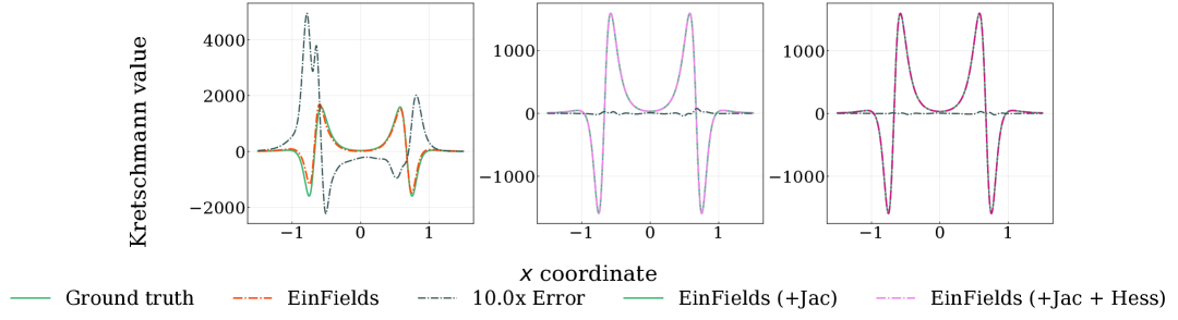
Figure 19: 2D Tomography of Kerr Kretschmann invariant in Cartesian KS representation.

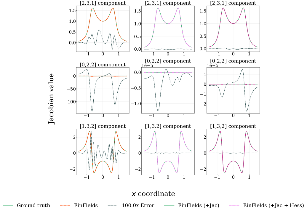
Figure 20: 2D Tomography of Kerr metric Jacobian components in Cartesian KS representation.

The impact of the modified training loss is particularly evident when accurately querying higher-order differential geometric quantities, which include the metric Jacobian, Christoffel symbols, metric Hessian, Riemann tensor, and curvature invariants on an arbitrary set of validation points. We evaluate the improvement in reconstruction quality and fidelity for these quantities on the Kerr metric in Cartesian KS coordinates, which are free of coordinate singularities, using 2D tomographic slices (see Section D.3 for details). Comparative results with and without Sobolev training are explicitly reported in Figures 20–19.

3.3.0.1 Reconstructing dynamics.

Reconstructing free-falling trajectories of bodies and light rays necessitates solving the geodesic equation (see Equation (71)). This requires the accurate computation of Christoffel symbols $\Gamma=\Gamma(g,\partial g)$. Moreover, Christoffel symbols are included in the covariant derivative $\nabla:=\partial+\Gamma$, playing a pivotal role in parallel transportation on (pseudo-) Riemannian manifolds (see Appendix A.3.3). Following our AD-based workflow depicted in Figure 3, EinFields (with Jacobian supervision) enable accurate AD-based reconstruction of the Christoffel symbols via $\Gamma\approx\hat{\Gamma}=\hat{\Gamma}(\hat{g},\partial\hat{g})$, and subsequently the covariant derivative operator $\nabla:=\partial+\hat{\Gamma}$. Consequently, we can model trajectories governed by the geodesic equation and also query the Riemann tensor ($\nabla\Gamma$, see Appendix A.3.5 for details) on arbitrary points.

3.3.0.2 Characterizing intrinsic geometry.

Beyond accurately capturing the spacetime dynamics, EinFields must also faithfully reproduce the intrinsic geometry of the underlying manifold. This intrinsic structure is encoded in key geometric quantities such as the Riemann curvature tensor, the Ricci tensor $R_{\alpha\beta}$, the Ricci scalar $R$, and the Kretschmann invariant (cf. Figure 3).

Our framework, trained with explicit supervision on Jacobian and Hessian fields, successfully meets these stringent geometric requirements. In particular, the learned fields demonstrate close quantitative agreement with their analytical counterparts across the computational domain. This fidelity holds especially well in regions sufficiently distant from zones of extreme curvature or curvature singularities, where numerical learning and representation are inherently more challenging. For a detailed analysis of curvature tensors and invariants computed by our model, see Appendix 2.

Figure 3: Automatic differentiation-enabled directed-acyclic graph (DAG) for computational differential geometry analogue of Figure 2. The diagram illustrates the computational workflow for constructing geometric quantities from a metric tensor $\mathtt{g}$. The metric’s Jacobian $\mathtt{Jac(g)}$ is obtained via forward-mode automatic differentiation (Jacfwd) and contracted using Einstein summation (Einsum) to compute the Christoffel symbols $\mathtt{\Gamma}$. Covariant derivatives and Lie derivatives utilize $\mathtt{Jacfwd\bigoplus\Gamma}$ emerging as derivative operators acting on tensors. The Riemann tensor $\mathtt{Riem}$ is built through further application of Jacfwd and $\mathtt{\Gamma}$, followed by contraction to yield the Ricci tensor $\mathtt{Ric}$ and scalar curvature $\mathtt{R}$. Branches compute the Weyl tensor $\mathtt{C}$ and enforce Bianchi identities $\big{(}\mathtt{Jacfwd\bigoplus\Gamma}\big{)}\mathtt{Riem}=0$. This framework leverages automatic differentiation and tensor algebra to enable scalable symbolic-numeric computations in geometric deep learning and physics-informed models.

4 Experiments

4.1 Evaluation criteria

We flatten the ground truth tensor at point $p\in\mathscr{M}$ with its components indexed by $k$ be denoted by $f_{k}(p)\in\mathbb{R}^{n}$, with $1\leq k\leq n$ and the corresponding EinFields parametrized tensors are denoted by $\hat{f}_{k}(p)$. The dimensionality $n$ depends on the tensor under consideration. For instance, for a symmetric metric tensor $n=10$, corresponding to its independent components, while for the Riemann curvature tensor, $n=256$ when considering all components explicitly, or $n=20$ when accounting only for the independent components under the symmetries inherent to the tensor, respectively.

We evaluated these quantities over a set of $m\approx 125,000$ validation collocation points $\mathcal{D}=\{p_{i}\}_{1\leq i\leq m}$ and use standard error criteria in discretized form, which includes double sums: one over the total number of tensor components $\{f_{k}\}_{1\leq k\leq n}$, while the other for the total number of collocation points $\{p_{i}\}_{1\leq i\leq m}$:

Mean-absolute error (MAE) $$=\frac{1}{mn}\sum_{i=1}^{m}\sum_{k=1}^{n}|\hat{f}_{k}(p_{i})-f_{k}(p_{i})|$$ (10a)

Relative $$\ell_{2} \ell_{2} =\sqrt{\dfrac{\sum_{i=1}^{m}\sum_{k=1}^{n}|\hat{f}_{k}(p_{i})-f_{k}(p_{i})|^{2}}{\sum_{i=1}^{m}\sum_{k=1}^{n}|f_{k}(p_{i})|^{2}}}\ .$$ error (Rel. ) (10b)

These are applied to the metric tenors and their derived quantities, illustrated in Figures 2 and 3. Recall that the tensor components are coordinate-dependent (and even more so, the metric Jacobian, metric Hessian, and Christoffel symbols are not even tensors), and, hence, these errors lack an immediate physical meaning. This is improved with the consideration of scalar quantities such as the Ricci scalar, Kretschmann invariants, and Weyl scalars, which by definition are coordinate-independent quantities.

The above error criteria are an aggregation of point-wise, i.e., local quantities. We additionally assess the quality of free-falling trajectories obtained by evolving the geodesic equation (Equation 2) from the same initial condition on the exact and approximate metrics. Even small errors quickly accumulate during the evolution of the trajectory, providing a sensitive assessment of the metric quality. In addition, these trajectories provide a strong physical intuition, e.g., the number of stable orbits.

4.2 Floating point precision

NR simulations are inherently high-precision endeavors, with the accurate modeling of complex gravitational phenomena critically reliant on high-fidelity numerical computations. In contrast to traditional machine learning domains, such as large language models (LLMs), where reduced-precision arithmetic (FLOAT16 or BFLOAT16) yields strong results in both training accuracy and memory efficiency (Dean et al., 2012), this paradigm does not extend to NR workflows, where floating-point precision is a dominant factor influencing the fidelity of the results.

While single-precision (FLOAT32) arithmetic is sufficient for training EinFields in most experiments and downstream tasks presented, geodesic simulations (see Figures 5 and 7) indicate the need for FLOAT64 precision results in MAE and relative $\ell_{2}$ error for the reconstructed metric and its derivatives. Only FLOAT64 ensures the mitigation of error accumulation during temporal rollout, preserving the accuracy necessary for reliable scientific inference in gravitational physics.

4.3 Data

Our use cases are exact analytic solutions to the EFEs, i.e., the set of metrics $g_{\alpha\beta}$ that satisfy the Equation (1). These solutions describe the exterior (vacuum) solutions around massive gravitating objects. For our main set of experiments, we fit a NeF against the analytic solutions introduced in Section 2.1.1, each having different features and spatio-temporal symmetries:

• Schwarzschild metric in spherical coordinates (Equation (113)),

• Kerr metric in Boyer-Lindquist and Kerr-Schild coordinates (Equations (116, 96)),

• gravitational waves metric (TT gauge) in Cartesian coordinates (Equation (100)).

For each, we compute the distortion after subtracting the flat background metric using the corresponding equations summarized in the Appendix. Detailed information on data specifications is provided in Table 1.

Additionally, in Section 4.7, we train each geometry in different coordinate systems to investigate how the choice of coordinates impacts NeFs (recall: the physical laws do not depend on the coordinate system).

Metric	Coordinates	Domain	Resolution	Parameters
Schwarzschild	Spherical $(t,r,\theta,\phi)$	$t=0$ $r\in$ [2.5,150] $\theta\in$ (0, $\pi$) $\phi\in[0,2\pi)$	1 128 128 128	M = 1
Kerr	Boyer-Lindquist $(t,r,\vartheta,\phi)$	$t=0$ $r\in$ [3,14] $\vartheta\in$ (0, $\pi$) $\phi\in$ [0, $2\pi$)	1 128 128 128	M = 1 $a\in$ [0.628,0.95]
	Kerr-Schild $(t,x,y,z)$	$t=0$ $x\in$ [-3, 3] $y\in$ [-3, 3] $z\in$ [0.1, 3]	1 128 128 128	M = 1 $a$ = 0.7
Linearized gravity	Cartesian $(t,x,y,z)$	$t\in$  [0, 10] $x\in$ [0, 10] $y\in$ [0, 10] $z\in$ [0, 10]	140 10 10 140	$\omega$ = 1 $\epsilon=10^{-6}$

Table 1: Training data generation specifications: spacetime metric, coordinate system, domain extent, grid resolution, and physical parameters.

4.4 Training

Across the experiments, we consider several NeF models. The most effective and accurate models for our use cases are MLPs with SiLU (i.e., sigmoid-weighted linear units) activation function  (Elfwing et al., 2018), which are especially suited when supervising over derivatives. Moreover, since the optimizer is known to impact the speed and convergence of the training strongly and subsequently the accuracy of the model (Wang et al., 2025), we utilize SOAP (Vyas et al., 2025), a scalable quasi-Newton method with consistently improved gradient alignment between losses in PINNs. However, since our training characteristics are different from PINNs, we do not expect SOAP to mitigate the problem of gradient conflict (see Appendix D.1) completely, but rather to leverage the second-order approximation combined with its advanced preconditioning and computational efficiency. That being said, using SOAP increases the optimization efficiency and reduces the training loss by at least two orders of magnitude compared to ADAM  (Kingma & Ba, 2015).

To mitigate gradient imbalances during Sobolev supervision, which is especially more pronounced in low- or high-curvature regions where the metric or its derivatives dominate, respectively, we adopt a gradient normalization weighting scheme (GradNorm (Chen et al., 2018)), forcing all gradients to unit norm. This is a slightly different weighting compared to Wang et al. (2020), in the sense that we do not multiply by the sum of the gradient norms, resulting, however, in better results for our use case.

The investigated MLP widths and depths range from $\mathtt{64\times 3}$ to $\mathtt{512\times 7}$, with less than $\mathtt{1.9\times 10^{6}}$ parameters ($\sim 7\mathtt{MiBs}$). We use the cosine annealing learning rate schedule, with the initial learning rate set to $\eta=$ 1E-2. The number of training epochs is chosen between $[\mathtt{100},\mathtt{200}]$, and the number of batches per epoch varies from 20 up to 300. The $\mathtt{100}$ epochs runs with $\mathtt{100}$ batches had a runtime $\sim\mathtt{20{it/s}}$ for metric alone to $\sim\mathtt{5{it/s}}$ including Hessian supervision. In wallclock time, this ranges between $64$ seconds for the former, and $2140$ seconds for the latter. For more details on the training hyperparameters, see Table 10.

4.5 Accuracy and storage efficiency of EinFields

In this work, we adopt finite difference (FD) methods as our baseline, recognizing their limitations relative to spectral approaches as detailed in Section 2.2. The integration of spectral techniques will be the focus of future work.

In Table 2, we report the representation capacity of EinFields and its Sobolev-enhanced variants (trained according to Pseudocode 1) on the distortion component of the Schwarzschild metric expressed in spherical coordinates (see Equation (113)).

We evaluate models using the discrete forms of the mean absolute error (MAE) and relative $\ell_{2}$ error as defined in Equations (10), achieving best-case accuracies of approximately $10^{-8}$ (MAE) and $10^{-7}$ (Rel. $\ell_{2}$) on validation points.

The last two columns of Table 2 report the memory efficiency of NeFs and the associated compression factors relative to explicit grid representations. Notably, while modifying the loss functions does not directly impact storage requirements, the resulting differences in accuracy across schemes lead to variations in effective storage/compression values, as we select the highest achievable accuracy for each method. These trade-offs are visualized in Figure 4(a), where the curves are obtained by connecting points to form decreasing trendlines.

Representation	Rel. $\ell_{2}$	MAE	Storage	Compression
EinFields	2.37E-7	3.93E-7	$\mathbf{85}$ KiB	$\mathbf{4035}$
EinFields (+ Jac)	1.51E-7	2.20E-7	$1.1$ MiB	$311$
EinFields (+ Jac + Hess)	1.40E-7	6.89E-8	$202$ KiB	$1698$
Explicit grid	$-$	$-$	$343$ MiB	$-$

Table 2: Performance evaluation (measured in Rel. $\ell_{2}$ and MAE metrics) and storage efficiency of EinFields parametrized metric tensor fields under different representations (i.e., with and w/o Sobolev trainings). The model with the lowest MAE is selected in each row.

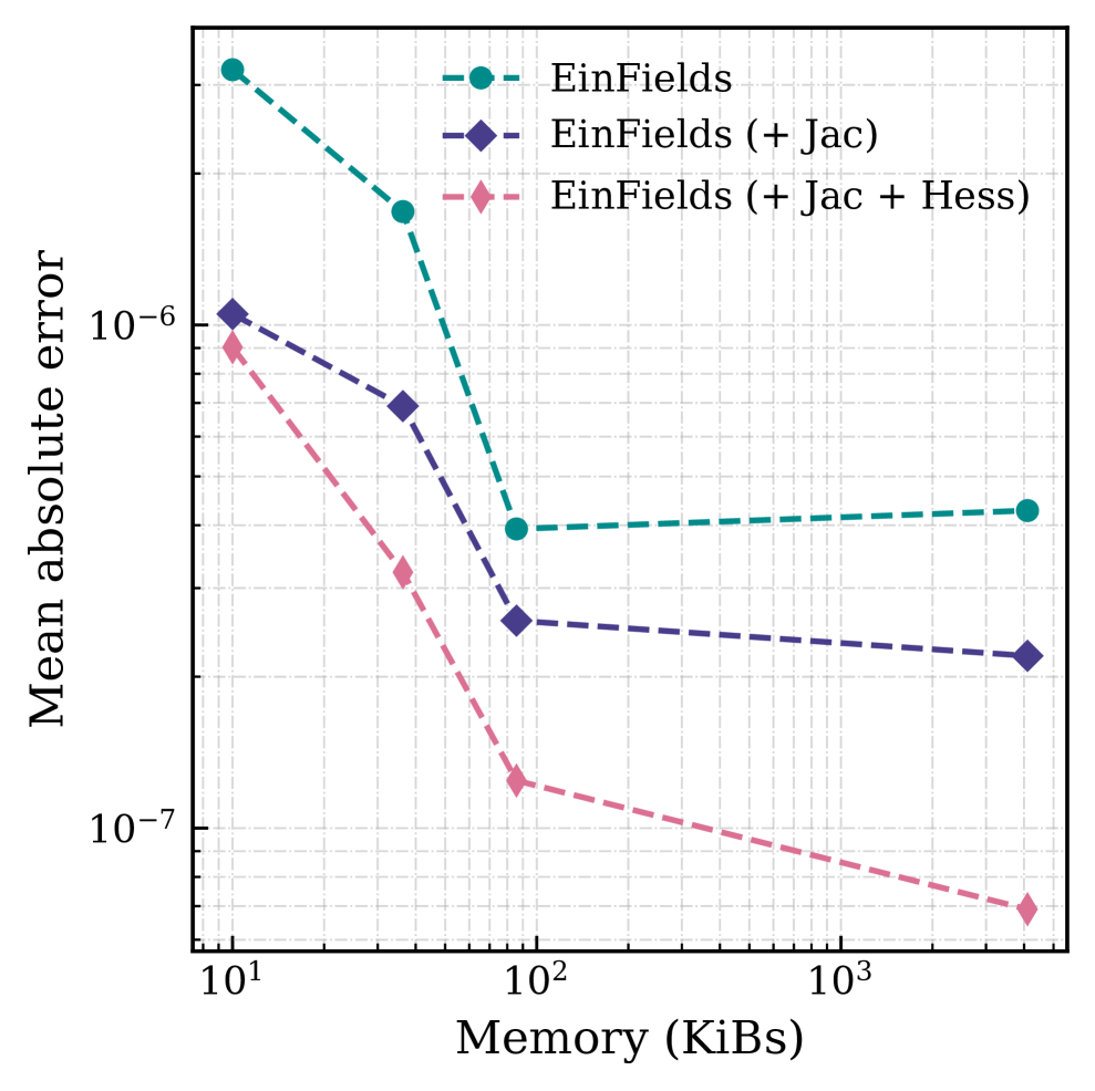
(a) Accuracy of EinFields for different NN sizes (measured in KiBs required to store all FLOAT32 parameters) as trendlines for different training schemes. Each metric tensor component has MAE values ranging from 1E-6 to 1E-8. Apart from high accuracy, one additionally acquires $\sim 1000-4000$ times compression factors in storage memory gain, as detailed in Table 2.

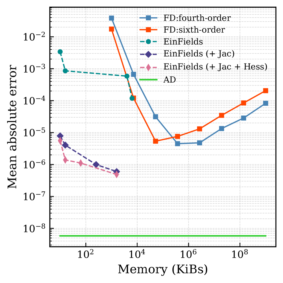
(b) Accuracy of EinFields’ Christoffel symbols derived from the metric tensor, shown as trendlines for different training schemes in FLOAT32 (KiBs). The trendlines show different training schemes (with and without Sobolev training) with MAE values ranging from 1E-4 to 1E-7. We benchmark against fourth-order and sixth-order stencils with truncation errors $\mathcal{O}(h^{5})$ and $\mathcal{O}(h^{7})$, respectively. Our framework outperforms FD stencils by more than an order of magnitude in accuracy.

Figure 4: Trendlines of accuracy versus storage memory (KiB) requirement for the metric tensor and Christoffel symbols. For the explicit grid storage this is computed as $\mathtt{num\ of\ grid\ collocation\ points\times 4}$, with 4 bytes for single precision ($\mathtt{FLOAT32}$). For the NeFs, this corresponds to the storage memory of the compact implicit NN weights.

4.5.0.1 Accuracy and storage efficiency of tensor differentiation.

High-fidelity reconstruction of higher-rank tensors that are obtained via differentiation of neural tensor fields is essential for accurately recovering the underlying physics, including geodesics, tidal forces, and related geometric quantities. Here, we evaluate the performance of our framework by reporting accuracy versus memory trendlines for the metric tensor (Figure 4(a)) and the Christoffel symbols (Figure 4(b), computed via AD). We apply the same setting as used for the results in Table 2. For the Christoffel symbols, the trendlines for the higher-order finite-differencing methodologies ($\mathtt{4}$-th and $\mathtt{6}$-th order stencils) are compared against EinFields and Sobolev training variants. While EinFields exhibits a decreasing MAE when plotted against increasing network sizes (# of floats), the FD baselines face notable limitations not only coming from truncation errors and numerical instabilities (increasing error for smaller $h$ values), but also accuracy and memory efficiency-related bottlenecks.

Furthermore, we report the performance of AD-based Jacobians and covariant derivative operators, through which we obtain Christoffel symbols (see Equation (64)), the Riemann curvature tensor (see Equations ((72), (73)), the contracted curvature tensors (Weyl tensor, Ricci tensor, Ricci scalar), and the curvature invariants (see Section 2). We compare against higher-order FD-stencils. Table 3 shows that EinFields reconstructed differential geometric quantities are up to $\mathtt{10-10^{5}}$ times more accurate than FD stencils for these differential geometric quantities.

Geometric quantity	Storage [GiB]		MAE
	Full	Sym.	GT (FD)	EinFields (AD)	GT (AD)
Christoffel symbol	26	16	5.37E-6	4.87E-7	5.83E-9
Christoffel Jacobian	103	64	6.24E-3	1.63E-6	1.71E-8
Metric Lie derivative	103	64	6.24E-3	1.63E-6	1.71E-8
Riemann tensor	103	8.0	1.78E-2	2.53E-7	2.86E-8
Weyl tensor	103	4.0	1.72E-2	5.71E-7	5.89E-8
Ricci tensor	6.5	4.0	4.81E-2	1.02E-6	9.02E-8
Ricci scalar	0.4	0.4	5.35E-2	5.66E-5	1.31E-8
Kretschmann invariant	0.4	0.4	1.33E-2	1.71E-5	3.32E-8

Table 3: Performance evaluation of EinFields reconstructed differential geometric quantities obtained for the Schwarzschild geometry in spherical coordinates. Column 1 reports values on a spherical grid with spacing $\mathtt{h=0.01}$. Columns 2 and 3 report memory usage when storing full and symmetry-reduced components, respectively. Column 4 shows the MAE from EinFields (AD) measured against analytical solutions. Bold entries indicate significant accuracy gains over naive finite-difference baselines applied on the ground-truth (GT) metric (GT (FD), $\mathtt{h=0.01}$). The last column (GT (AD)) applies AD to the analytic solution, which almost coincides with the analytic expressions for these differential geometric quantities.

4.6 Reconstructing general relativistic dynamics and curvature scalars

We use synthetic data generated from analytical solutions to validate and characterize EinFields. We primarily focus on two interesting aspects of general relativity: (i) general relativistic dynamics, particularly geodesic motion around massive gravitating objects (see Section 2.1.0.8) and (ii) global curvature structures encoded in tensorial invariants.

4.6.0.1 EinField-based geodesics.

To compute geodesic motion, we numerically integrate the trajectories using a fifth-order explicit singly diagonally implicit Runge-Kutta (ESDIRK) solver. Specifically, we evolve Equation (2) with respect to the affine parameter $\tau$ (proper time),generating ground-truth geodesics from the analytic Christoffel symbols for the Schwarzschild and Kerr spacetimes. These are then compared against the rollouts obtained using the EinField-reconstructed Christoffel symbols.

To accurately retrace geodesic orbits, it is essential to incorporate Jacobian supervision within the Sobolev training framework. In contrast, additional Hessian supervision results in only marginal improvements for geodesic simulations and is not required in practice. Following Section 4.2, all geodesic solvers are executed in double precision to ensure numerical stability and high-fidelity trajectory reconstruction.

Following the strategy presented in Section 3.3, we leverage EinFields’ ability to yield high-precision derivatives of the spacetime metric, which includes Christoffel symbols, Riemann curvature tensors, and scalar invariants. In this section, we demonstrate how to accurately model particle trajectories derived from geodesic integration with our implicit parameterizations.

4.6.1 Schwarzschild metric

Geodesics in the Schwarzschild spacetime are of fundamental interest, as they underlie phenomena such as gravitational lensing and the perihelion precession of Mercury, as well as the motion of planets in the solar system more generally.

The initial conditions of the trajectories chosen in the experiments are fully specified by the initial position

$$(t,r,\theta,\phi)(t=0)=\big{(}0,a_{0}r_{s},\pi/2,0\big{)}$$ (11)

and the initial four-velocity

$$(v^{t},v^{r},v^{\theta},v^{\phi})(t=0)=\big{(}\frac{1}{\sqrt{(1-r_{s}/r_{0})(1-v_{0}^{2})}},0,0,v_{0}\frac{\cos\phi_{0}}{\sqrt{r_{0}^{2}(1-v_{0}^{2})}}\big{)}\ ,$$ (12)

Where $v_{0}=b_{0}\sqrt{1/(r_{0}-r_{s})}$ and $a_{0},b_{0}\in\mathbb{R}$ can be chosen freely to select the desired orbit in the $\theta=\pi/2$ plane. The geodesics in Figure 5 demonstrate a good qualitative agreement over several orbits. The error is quantified and discussed further in Section 4.8.

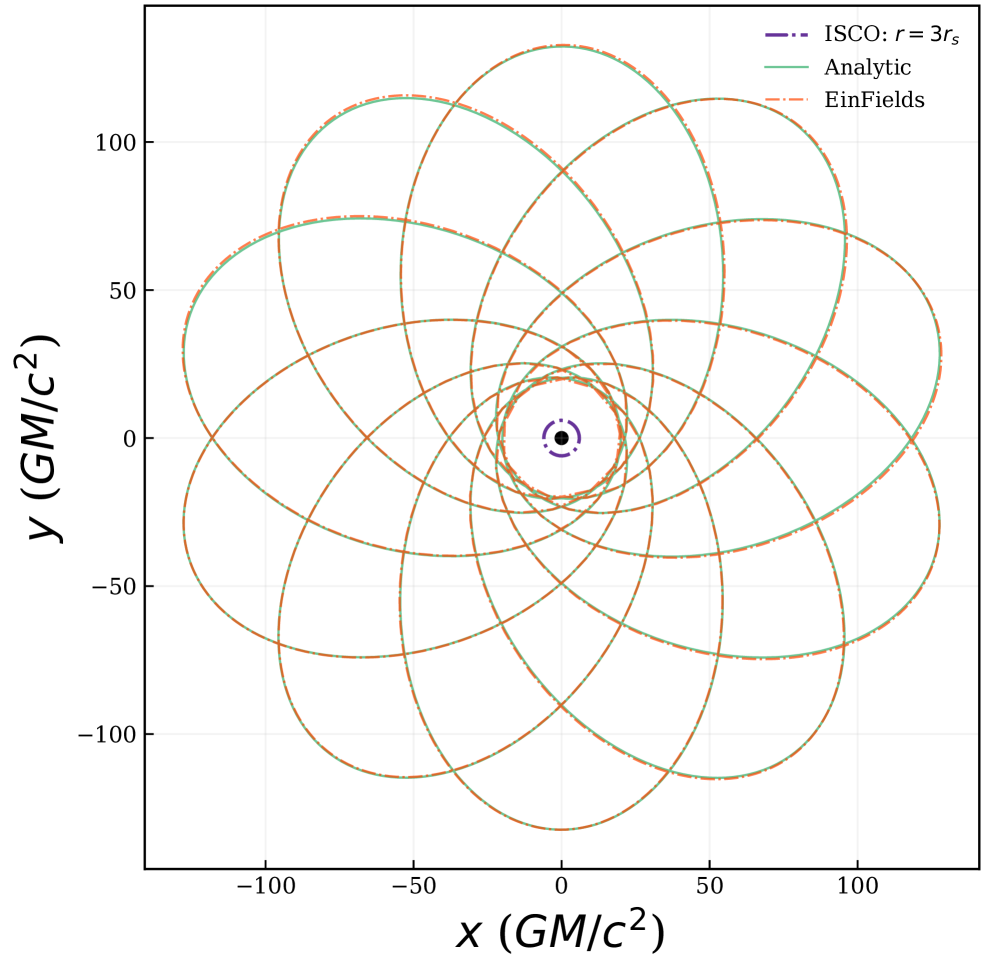
(a) Perihilion precession orbits.

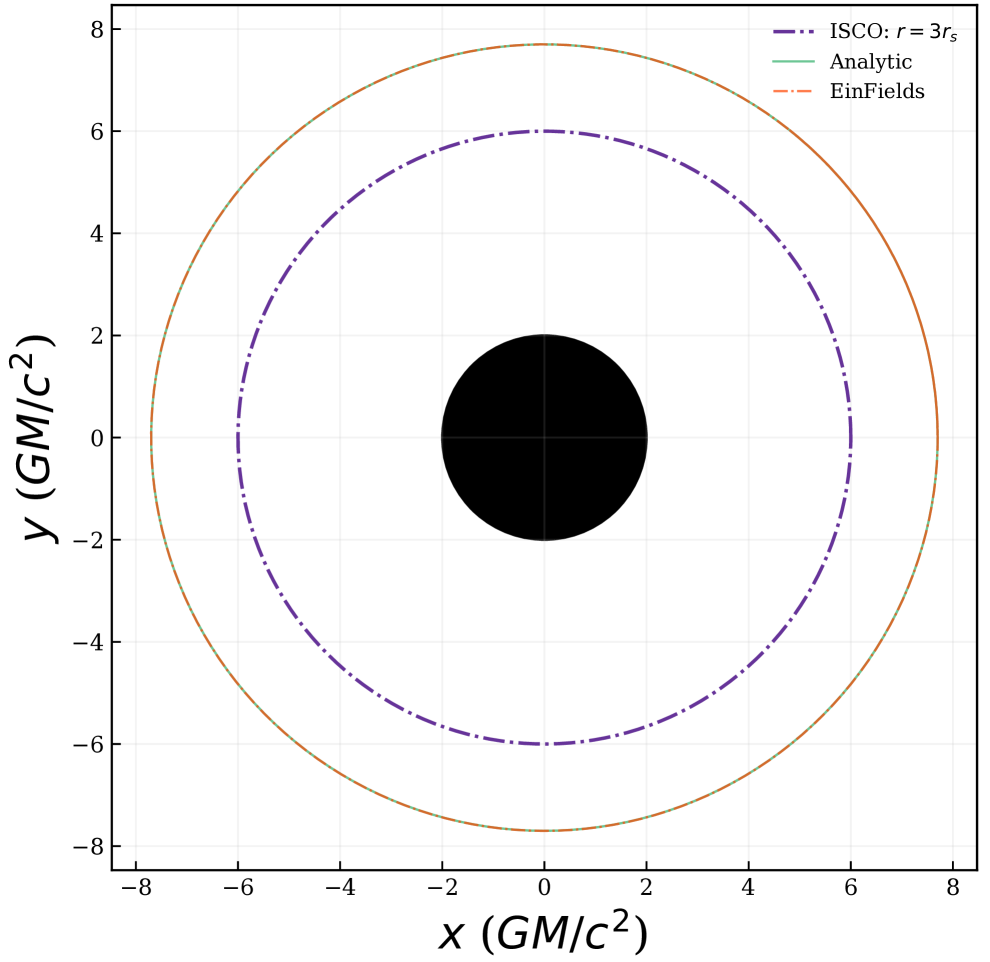
(b) Circular orbit for $r=3.85r_{s}$.

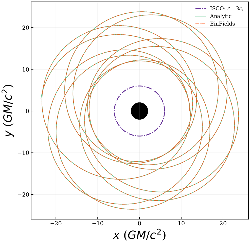
(c) Eccentric orbits.

Figure 5: Geodesics in Schwarzschild spacetime simulated in spherical coordinates (Equation (85)). The filled black circle indicates $r\leq r_{s}=2M$. The purple dashed line marks the innermost stable circular orbit (ISCO) at $r=3r_{s}$. Green solid lines represent the ground-truth geodesics, while the red dotted lines represent EinFields reconstructed ones. We find very close agreement between the orbits up to a chosen time of running the geodesics.

Being able to compute geodesics is sufficient to perform rendering. We use the Schwarzschild EinFields metric to render a black-hole on a celestial background. This requires propagating geodesics from the camera observer via the spacetime terminating at the distant background. The resulting image in Figure 6 provides visual evidence for the global consistency and quality of the metric and the derived Christoffel symbols.

Figure 6: Render of a Schwarzschild black-hole in front of a celestial background constructed from the EinField metric.

4.6.2 Kerr metric

Geodesics in a Kerr spacetime around a rotating body (see details in Appendix B.2) play a central role in several key astrophysical observations and experimental tests of GR. Notably, photon geodesics determine the black hole shadow images captured by the Event Horizon Telescope (Fuerst, S. V. & Wu, K., 2004), and frame-dragging (Lense-Thirring) effects (Misner et al., 2017) are a hallmark of the Kerr geometry. These have been measured experimentally by the Gravity Probe B mission (Everitt et al., 2011) and recently via radio pulses arriving from pulsars (Krishnan et al., 2020).

We consider three different cases, namely, Zackiger orbits (retrograde geodesics – stable geodesics with larger radii), prograde orbits (stable geodesics with smaller radii), and arbitrary eccentric orbits, which depend on the initial conditions, including choice of energy $E$ and angular momentum $L_{z}$ of the test particle. The geodesics in Figure 7 demonstrate a good qualitative agreement over several orbits. The error is quantified and discussed further in Section 4.8.

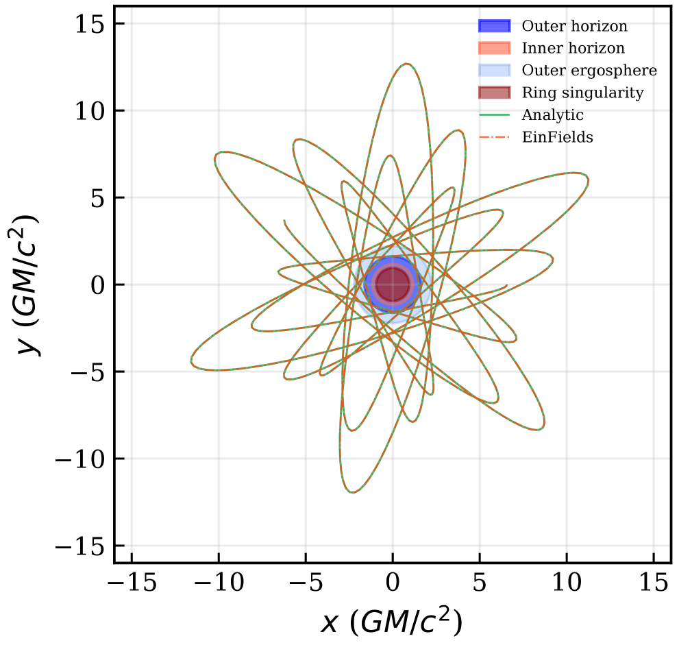
(a) Retrograde orbit for $a=0.95$.

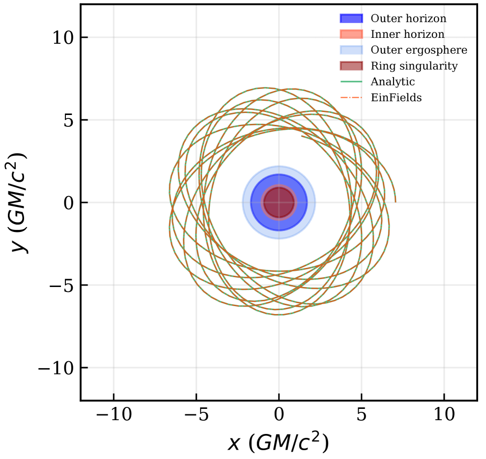
(b) Prograde orbit for $a=0.90$.

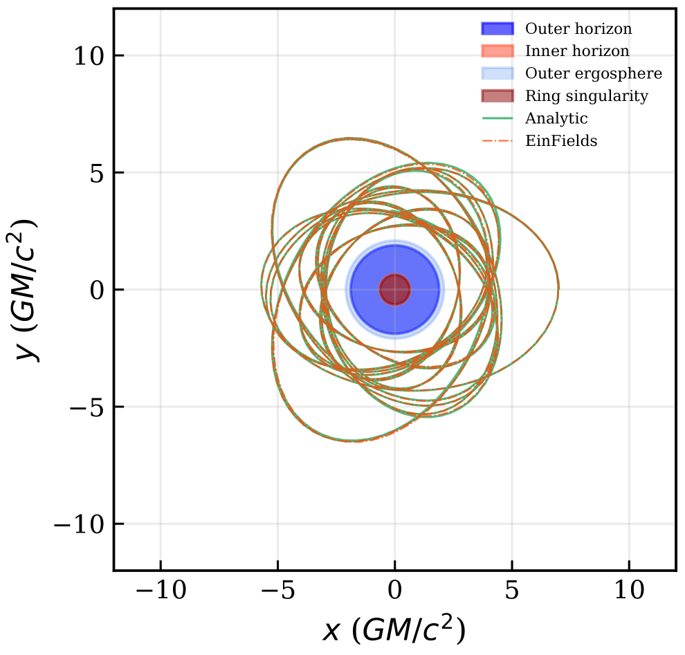
(c) Eccentric orbit for $a=0.628$.

Figure 7: Geodesics in Kerr spacetime simulated in Boyer–Lindquist coordinates (Equation (95)). Distinct regions of the geometry are indicated in solid colors. Green solid lines represent ground-truth geodesics, while the red dotted lines represent our NeFs reconstructed orbits.

Kretschmann invariant. The Kretschmann invariant (scalar), $\mathscr{K}=R^{\alpha\beta\gamma\delta}(x^{\mu})R_{\alpha\beta\gamma\delta}(x^{\mu}),$ is a key curvature invariant distinguishing true (curvature) singularities from coordinate (apparent) singularities (see Appendix A.3.5.5). For the Kerr geometry, the rotation parameter $a$ induces a ring singularity at radius $a$ on the equatorial plane $\theta=\pi/2$, where the curvature diverges (see Equation (99) and Section B.2.2). Accurately capturing this geometric structure requires isolating true singularities from coordinate artifacts, which can otherwise lead to incorrect classification of singularities.

We perform training in Cartesian KS coordinates (see Equation (96)) to eliminate coordinate singularities that would otherwise impede convergence. We first train EinFields (+Jac + Hess) on Cartesian KS coordinates, subsequently constructing the Riemann tensor (see Section A.3.5) via successive automatic differentiation steps and raising indices using the parametrized metric $\hat{g}$ (see Equation (99)). The NeF reconstructed $\hat{\mathscr{K}}$ captures the ring singularity structure and agrees well with the analytical solution, as shown in Figures 8(a) and 8(b). However, the reconstruction remains sensitive to floating-point errors and requires high NeF accuracy for stability (see Limitations, Section 5.0.0.1).

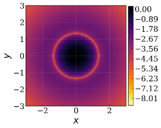
(a) Analytic form $\mathscr{K}$

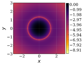
(b) EinFields reconstructed $\hat{\mathscr{K}}$

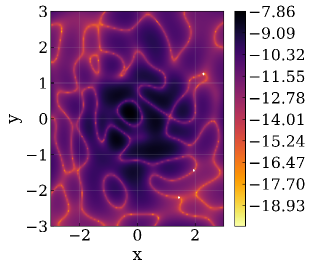
(c) Absolute error $|\mathscr{K}-\hat{\mathscr{K}}|$

Figure 8: The Kretschmann scalar $\mathscr{K}$ of the Kerr metric computed in Cartesian Kerr-Schild form (Equation (96)) in the $x$-$y$ plane for $z=0.3$.

4.6.3 Linearized gravity

Linearized gravity models the solution of the EFEs via periodic perturbations on a fixed background metric. These linearized solutions are highly relevant in numerical relativity, as they describe the groundbreaking, experimentally verified discovery of gravitational waves generated by binary black hole mergers  (Abbott et al., 2016c). The metric tensor can be written as

$$g_{\alpha\beta}\approx\eta_{\alpha\beta}+h_{\alpha\beta}+\mathcal{O}(h_{\alpha\beta})^{2}\ ,$$ (13)

where $|h_{\alpha\beta}|\ll 1$ is the perturbation term. As detailed in Section B.3, a plane gravitational wave propagating in the $z$-direction with angular frequency $\omega$ can be described in the tranverse-traceless (TT) gauge as

$$h_{\alpha\beta}^{\text{TT}}=\begin{pmatrix}0&0&0&0\\ 0&h_{+}&h_{\times}&0\\ 0&h_{\times}&h_{+}&0\\ 0&0&0&0\end{pmatrix}\cos\big{(}\omega(t-z)\big{)}\ .$$ (14)

Here, $h_{+}$ and $h_{\times}$ are the amplitudes of the “$+$” (plus) polarization and “$\times$” (cross) polarization.

4.6.3.1 Validation problems for GW metric and derivatives quality.

Compared to Schwarzschild and Kerr metrics, a key distinction of the linearized gravity setting describing gravitational waves is its time dependence (see Equation (100)). Although it does not depend on $x$ and $y$, the temporal dependence motivates us to consider our model trained on a full spacetime grid of size $\mathtt{N_{t}\times N_{x}\times N_{y}\times N_{z}}$.

4.6.3.2 Distortion of ring of test-particles.

When the described gravitational wave interacts with a ring of freely falling test particles initially at rest in the x-y plane, it induces periodic deformations of the ring. For a purely $+$ polarized wave, the resulting motion causes the ring to stretch and squeeze along the x- and y-axes, leading to a characteristic “plus” deformation pattern.

The motion of the test particles under the influence of this gravitational wave is obtained by solving the geodesic deviation equation, up to leading order in the strain amplitude $h_{+}$. As a result, the particle trajectories in the TT gauge are

$$x(t)=\bigg{(}1+\frac{1}{2}h_{+}\cos\big{(}\omega(t-z)\big{)}\bigg{)}x(0)\ ,\ y(t)=\bigg{(}1-\frac{1}{2}h_{+}\cos\big{(}\omega(t-z)\big{)}\bigg{)}y(0)\ .$$ (15)

Here, $x(0)$ and $y(0)$ denote the initial coordinates of a test particle, and the time-dependent perturbations reflect the tidal nature of gravitational waves. The cosine dependence captures the periodic stretching and squeezing of spacetime caused by the wave as it traverses the particle ring. Figure 9 and Table 6 show how the famous ring oscillation experiment can be reproduced with EinFields. This is done by parametrizing the perturbation $h_{\alpha\beta}^{\text{TT}}$ and captures the famous stretching and squeezing effect.

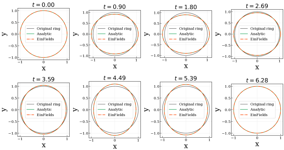
Figure 9: Spatial deformations (stretching and squeezing) of a circular ring of test particles due to “+” polarization. The NeF-parametrized perturbation terms $h_{+}\cos\big{(}\omega(t-z)\big{)}$ and $h_{\times}\cos\big{(}\omega(t-z)\big{)}$ show excellent agreement with the analytic result in the linearized gravity use case. See Table 6 for a quantitative evaluation.

4.6.3.3 Weyl scalars of gravitational radiation field.

The Weyl scalars are five complex quantities $\Psi_{0},\Psi_{1},\Psi_{2},\Psi_{3},\Psi_{4}$ that arise in the Newman–Penrose formalism of GR (Newman & Penrose, 1962). They encode all the independent components of the Weyl tensor $C_{\alpha\beta\gamma\delta}$ (see Equation (78)), representing the “free” gravitational field – the part of spacetime curvature that can propagate as gravitational waves, distinct from the curvature directly caused by matter. In NR and GW modeling, $\Psi_{4}(t)$ is the primary scalar quantity used to extract observable GW signals from simulations. It is defined as

$$\Psi_{4}:=C_{\alpha\beta\gamma\delta}n^{\alpha}\bar{k}^{\beta}n^{\gamma}\bar{k}^{\delta}$$ (16)

with $n,k$ being a particular choice of Newman–Penrose tetrads and $\bar{k}$ its complex conjugate . The central relation in an asymptotically flat spacetime (cf. Boyle et al. (2019) for details) is that $\Psi_{4}(t)$ is equivalent to the second coordinate-time derivative of the strain $h(t)=h_{+}(t)+ih_{\times}(t)$:

$$\Psi_{4}\equiv-\ddot{h}_{+}+i\ddot{h}_{\times}\ .$$ (17)

We compute $\Psi_{4}$ from the NeF-parameterized strain $h_{\alpha\beta}$ in two distinct ways:

1. indirectly via the Weyl tensor obtained with the differential-geometric chain (see also Figures 2 and 3): $h_{\alpha\beta}^{\text{TT}}\xrightarrow{+\eta_{\alpha\beta}}g_{\alpha\beta}\xrightarrow{\partial}\Gamma^{\gamma}_{\alpha\beta}\xrightarrow{\nabla}R^{\delta}_{\ \alpha\beta\gamma}\xrightarrow{}C_{\alpha\beta\gamma\delta}\xrightarrow{\text{Eq. \eqref{eq:weyl_scalar4}}}\Psi_{4}$;

2. directly via the second time-derivative: $h_{\alpha\beta}^{\text{TT}}\xrightarrow{\text{Eq. \eqref{eq:weyl_scalar4_ddot}}}\Psi_{4}$.

4.6.3.4 Spin-weighted spherical harmonic representation for GW extraction.

A quantity of central interest in gravitational waveform construction is the mode decomposition of the GW strain into its angular components. The complex strain $h(t,r,\theta,\phi)\equiv h_{+}(t,r,\theta,\phi)-i\,h_{\times}(t,r,\theta,\phi)$ can be expanded in terms of spin-weighted spherical harmonics (SWSHs) as

$$h(t,r,\theta,\phi)=\dfrac{M}{r}\sum_{\ell=2}^{\infty}\sum_{m=-\ell}^{\ell}h^{\ell,m}(t)\,{}_{-2}Y_{\ell m}(\theta,\phi)\ ,$$ (18)

where ${}_{-2}Y_{\ell m}(\theta,\phi)$ are the SWSHs (see Equation (105)) with spin-weight $s=-2$ reflecting the helicity of GWs in the TT gauge (see Equations (103) and (104)). In practice, the dominant contributions to the strain arise from the quadrupole $(\ell=2,m=\pm 2)$ modes, denoted by $h^{2,\pm 2}(t)$, which capture the leading-order gravitational radiation (detailed in Section B.3.0.1). Figure 10

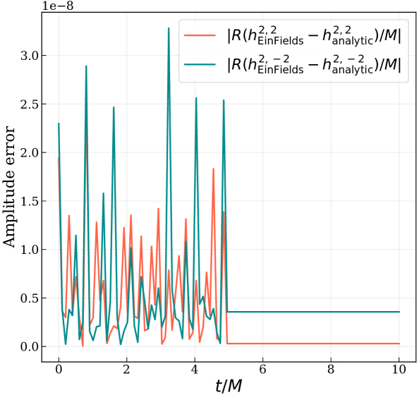
Figure 10: The absolute error of the amplitude between the EinFields and analytic values $|R/Mh^{2,\pm 2}(t)|$ (see Equation (104)) at a fixed radial distance $R=1$ plotted against $t/M$. The amplitudes agree to 1E-8, indicating that EinFields can capture the complex strain $h$ and subsequently $h^{2,\pm 2}(t)$ GW signals.

4.6.3.5 Radiated power of GWs.

Another important physical observable for GWs is the radiated power loss given by the famous quadrupole formula (Carroll et al., 2004). The time-averaged power or luminosity radiated by GWs is given by

$$\dfrac{\mathrm{d}E}{\mathrm{d}t}=\frac{r^{2}}{32\pi}\int\ \mathrm{d}\Omega\langle\dot{h}^{TT}_{ij}\dot{h}^{TT\ ij}\rangle=\dfrac{1}{4}\langle\dot{h}_{+}^{2}+\dot{h}_{\times}^{2}\rangle\ .$$ (19)

The particular perturbation metric in the above experiments (see Equation (100)) has equal amplitude $A=h_{+}=h_{\times}$ for both $+$ and $\times$ polarizations. As a consequence, the radiated power loss simplifies to

$$\frac{\mathrm{d}E}{\mathrm{d}t}=\frac{\omega^{2}A^{2}}{4}.$$ (20)

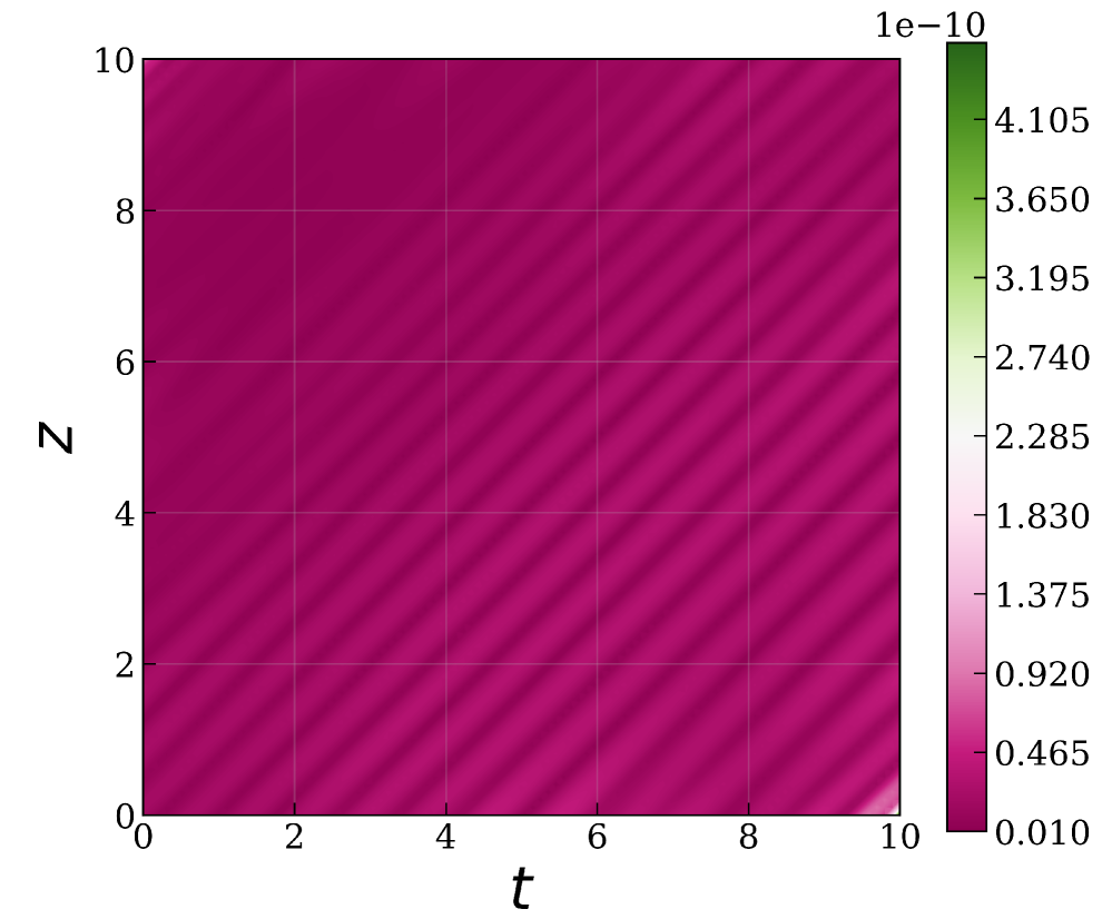
(a) Absolute error in the $(z,t)$ plane, averaged over $x$–$y$ slices.

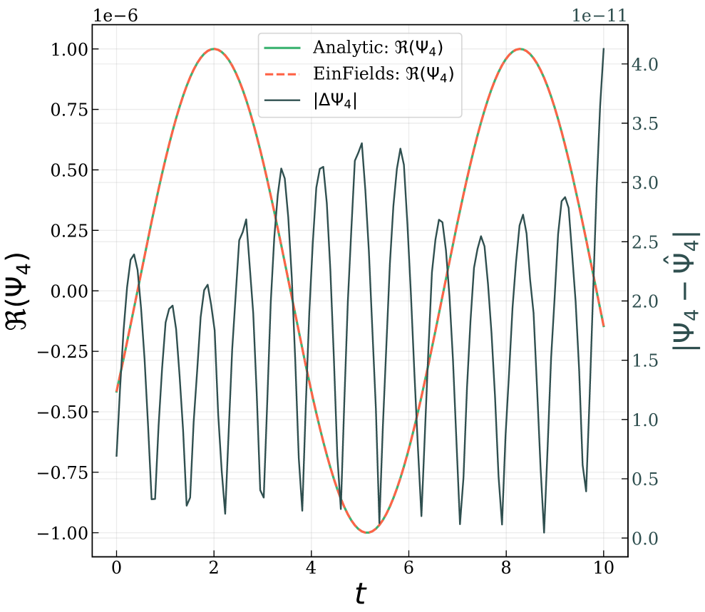
(b) Temporal evolution of the Weyl scalar computed from the analytic and EinFields perturbations (left axis) and their absolute error (right axis) at a fixed position.

Figure 11: Comparison of the real part of the Weyl scalar $\Re(\Psi_{4})$ (Equation (16)) computed from the EinFields and the analytic metric. The errors are on the order of E-10 and E-11, respectively, indicating highly accurate gravitational waveform reconstruction capacities of EinFields. Refer to Table 6 for more details.

4.7 Training on varied coordinate charts

The freedom to choose coordinate systems for describing spacetime geometries is a fundamental aspect of both theoretical GR and computational pipelines in NR. Consequently, it is essential to investigate how coordinate-dependent neural networks, i.e., NeFs, perform across input query coordinates that represent the same spacetime point $p\in\mathscr{M}$ when parameterized in different coordinate charts. To this end, we train EinFields on a range of coordinate systems for Schwarzschild and Kerr spacetimes, enabling a systematic examination of the impact of coordinate systems.

We compare the performance of EinFields on the Schwarzschild and Kerr metrics, since each of them possesses different families of coordinate charts (spherical-like, Cartesian-like, and lightcone-like) representations, as shown in the Table below: Furthermore, a detailed analysis and numbers pertaining to validation are reported in Appendix D.4.

Metric	Spherical-like	Cartesian-like	Lightcone-like
Schwarzschild	✓	✓	✓
Kerr	✓	✓	✓

Table 4: Col. 1 lists the spacetime metrics (Schwarzschild and Kerr). Cols. 2–4 indicate the coordinate charts used for NeF training: spherical-like, Cartesian-like, and lightcone-like. For Schwarzschild, these correspond to spherical coordinates $(t,r,\theta,\phi)$, Cartesian Kerr-Schild (KS) coordinates $(t,x,y,z)$, and ingoing Eddington-Finkelstein (EF) coordinates $(v,r,\theta,\phi)$, trained on the metrics described in Equations ((113))–((115)) respectively. For Kerr, these correspond to Boyer-Lindquist (BL) coordinates $(t,r,\vartheta,\phi)$, Cartesian KS coordinates $(t,x,y,z)$, and ingoing EF coordinates $(v,r,\theta,\tilde{\phi})$, trained on the metrics in described in Equations ((116))–((117)) respectively.

Results reported in Table 9 suggest that the choice of coordinates has a strong impact on the metric up to three orders of magnitude. This aspect should be investigated further in future work.

4.8 Accumulation of rollout errors for geodesics

Minute floating-point inaccuracies (around 1E-5 to 1E-6) arising from Christoffel symbols retrieved via EinFields autoregressively accumulate when evolving the equations of motion for test particles along geodesics.

To quantify the inaccuracies between the ground truth and NeF-evolved geodesics, we compute the deviation between the position vectors $r(\tau)\in\mathbb{R}^{3}$ as a function of the affine parameter (proper time) $\tau$ in Cartesian coordinates. Specifically, for the ground truth trajectory, the spatial coordinates corresponding to the position vector are given by $r(\tau)=\bigl{(}x(\tau),y(\tau),z(\tau)\bigr{)},$ while for the NeF-evolved trajectory, we denote $\hat{r}(\tau)=\bigl{(}\hat{x}(\tau),\hat{y}(\tau),\hat{z}(\tau)\bigr{)}.$ The deviation at each proper time $\tau$ is then computed as the Euclidean norm,

$$\delta r(\tau)=\left\|r(\tau)-\hat{r}(\tau)\right\|_{2}=\sqrt{\bigl{(}x(\tau)-\hat{x}(\tau)\bigr{)}^{2}+\bigl{(}y(\tau)-\hat{y}(\tau)\bigr{)}^{2}+\bigl{(}z(\tau)-\hat{z}(\tau)\bigr{)}^{2}}.$$ (21)

In practice, the geodesic trajectories are computed in $(r,\vartheta,\phi)$ (e.g., Boyer–Lindquist) coordinates and subsequently transformed into Cartesian coordinates before evaluating the deviation using the above expression.

Given the high sensitivity of time-stepped trajectories to such numerical inaccuracies, we quantify this error accumulation by explicitly presenting the deviation as a function of the affine parameter $\tau$, especially for eccentric orbits for both Schwarzschild (see Figure 5(c)) and Kerr metric for $a=0.628$ (see Figure 7(c)). These are reported for the Schwarzschild use case in Figure 12(a), and Figure 12(b) for the Kerr metric use case, respectively. For Schwarzschild, the error accumulates stably, while for Kerr it is erratic. We hypothesize this is likely due to the stable versus chaotic nature of orbits in the respective spacetimes. Eventually, orbits diverge significantly, especially when leaving the NeF training domain.

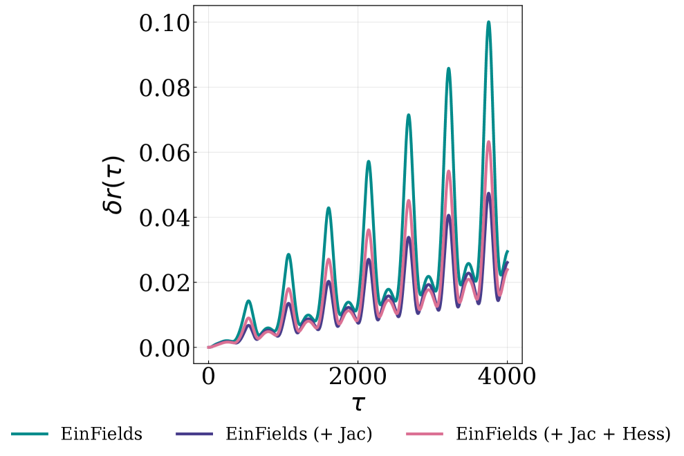
(a) Schwarzschild eccentric orbits.

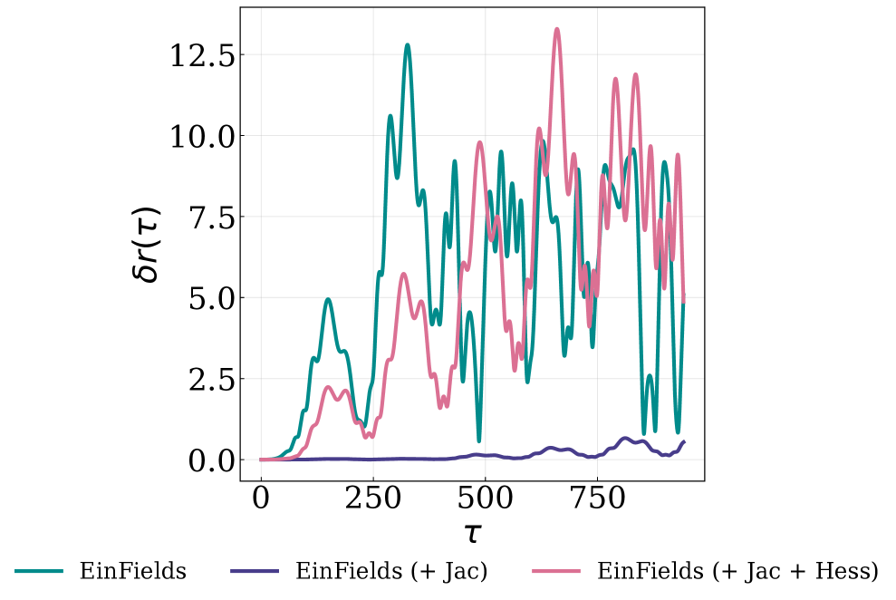
(b) Kerr eccentric orbits for $a=0.628$.

Figure 12: Geodesic rollout deviation $\delta r$ over proper time $\tau$.

The results suggest that incorporating the Hessian supervision into training may introduce noise that can hinder convergence, performing worse than using metric Jacobian supervision or, for that matter, metric alone. For geodesic equations, supervising second derivatives is often unnecessary, and Jacobians alone provide significant improvements in trajectory reconstruction. However, Hessians become essential when computing Riemann tensors and curvature-related quantities, and are required in applications such as numerically solving the geodesic deviation equation (see Equation (3)), which are typically encountered for solving for the test ring oscillation in linearized gravity use cases.

4.9 Ablation studies

4.9.1 Schwarzschild

We report detailed ablation results relative to our best-performing baseline configuration, systematically examining the effects of matrix representations (full metric instead of distortions), activation functions, optimizers, learning rate schedulers, and Sobolev regularization. All evaluations are conducted on spherical coordinates.

Ablation	Rel $\ell_{2}$	Wallclock time [s]
Baseline:   Metric distortion, Jac + Hes, SiLU, SOAP, Cosine LR	1.40E-7	1400
Metric distortion $\Delta_{\alpha\beta}$ $\rightarrow$ Metric $g_{\alpha\beta}$	2.13E-6	1407
Cosine $\rightarrow$ Const. LR	2.37E-5	1397
SOAP $\rightarrow$ ADAM	4.16E-6	1150
SiLU $\rightarrow$ WIRE	4.12E-6	3045
Jac + Hes $\rightarrow$ Jac	1.51E-7	509
Jac + Hes $\rightarrow$ -	2.37E-7	364

Table 5: Ablation study results for the Schwarzschild metric. Row 1: Best-performing configuration across all grid ranges (Full config). Row 2: Equation (85) in place of Equation (113)). Row 3: Constant learning rate versus cosine annealing schedule. Row 4: ADAM optimizer in place of the default SOAP optimizer. Row 5: Baseline activation (WIRE) compared to our proposed SiLU activation. Rows 6–7: Omitted Sobolev training (only Jacobian supervision or no higher-derivative supervision) on the full Schwarzschild metric. Column 2 reports the Rel $\ell_{2}$ error for the aforementioned rows. Column 3 reports the wall-clock time (seconds) required for training over 100 epochs (100 batches per epoch).

4.9.2 Linearized gravity

For GW tasks, we also compare against two other relevant models, which utilize periodic activations functions: (i) WIRE architecture (Saragadam et al., 2023) with a continuous real Gabor wavelet activation function $\psi(x;\zeta_{0},s_{0})=\cos(\zeta_{0}x)e^{-(s_{0}x)^{2}}$, with $\zeta_{0}$ and $s_{0}$ controlling the frequency of the wavelet and the spread, respectively (i.e., signal width localized in both the spatial and frequency domains), and (ii) SIREN (Sitzmann et al., 2020) architecture with the periodic activation function $\sin({\zeta_{0}x})$, and $\zeta_{0}$ being the modulating frequency.

The SiLU activation function exhibits a lower frequency bias and lacks oscillatory behavior in its higher-order derivatives, which directly feature in the Sobolev norms used during training. In contrast, sinusoidal activations employed in SIREN and WIRE architectures inherently possess oscillatory behavior, with their $k$-th derivatives scaling as $\zeta_{0}^{k}$, where $\zeta_{0}$ denotes the base frequency. This scaling amplifies high-frequency components and can lead to instability when minimizing Sobolev norms, as high-frequency errors become disproportionately emphasized. In practice, the smoothness and non-oscillatory nature of SiLU activations result in more stable training and improved generalization under Sobolev training objectives. These trends are quantitatively reflected in our experiments, as reported in Table 6.

Model	$h_{\alpha\beta}^{TT}$ (+Jac + Hess) (GradNorm)	Ricci scalar $R$	Weyl scalar $\Re(\Psi_{4})$	Luminosity $\mathrm{d}E/\mathrm{d}t$
SiLU	8.56E-4	5.90E-13	2.53E-5	2.71E-4
SIREN	3.78E-2	1.08E-12	9.56E-5	3.34E-4
WIRE	1.68E-2	1.55E-13	1.81E-5	3.69E-4

Table 6: Rel. L2 for key quantities in the linearized gravity case with two different NeF architectures: (i) perturbation metric, (ii) perturbation metric trained with Sobolev loss and gradient normalization, (iii) reconstructed Ricci scalar, and (iv) reconstructed real part of the Weyl scalar $\Psi_{4}$, where $\Psi_{4}\propto\ddot{h}_{+}(t,\mathbf{x})$. The final column reports the absolute difference in the predicted gravitational radiation energy loss, integrated over the unit sphere.

5 Conclusion

We have introduced Einstein Fields, short EinFields, which enable an efficient and differentiable modeling of 4D spacetime. EinFields leverage the concept of neural tensor fields together with the simplicity and stability of automatic differentiation, offering a scalable, discretization-free, and storage-efficient framework for physics observables encountered in GR. We have tested EinFields across several canonical test beds of GR, observing strong potential in terms of efficiency, storage requirements, accuracy, and faithful modeling of physics. We release an open-source JAX-based library, paving the way for future developments in NR: https://github.com/AndreiB137/EinFields.

5.0.0.1 Limitations.

The current main limitation stems from the lossy compression of NeFs. This prevents pushing the MAE of the metric components beyond $\mathtt{1E{-8}}$, outperforming the FD-methods only in the FLOAT32 setting. Despite using FLOAT64 training, our models cannot fit beyond $\mathtt{1E{-8}}$ MAE. These errors propagate over to the Christoffel symbol components, affecting the geodesics over long temporal rollouts of the geodesic solvers (see Figure 7(c)) for diverging orbits) and subsequently to the curvature tensors. Moreover, NeFs suffer near singularities, e.g., $1/|\mathbf{r}|$, and are unable to fit near-divergent points on a manifold. This and the aforementioned accumulation of floating point errors become even more pronounced for differential geometric quantities such as Kretschmann scalars, especially within spatial domains of high curvatures (see Figure 8(c)). Furthermore, since NeFs are coordinate-based NNs, training can be influenced by different choices of the basis sets and coordinate systems. Consequently, metric components may have different polynomial orders. For instance, in the spherical coordinate Schwarzschild metric $g_{\theta\theta},g_{\phi\phi}\propto r^{2}$, whereas, $g_{tt}\propto 1/r$. Thus, finding a NeF architecture, including the choice of activation functions that fit the metric tensor field in different coordinate systems, is a challenging task.

5.0.0.2 Future work.

The litmus test of EinFields is large NR simulation data, including spirals and merger events of binary black holes or binary neutron stars. Furthermore, our neural implicit frameworks should be tested against adaptive mesh refinement baselines, and recent developments in NR, such as the Discontinuous Galerkin (DG) method and classical discretization-free representations, such as (pseudo) spectral methods that are known to be orders of magnitude more efficient than FD (see Section 2.2.0.1). While the primary focus of this work is on the representation, NR can benefit from a hybrid framework that combines NeFs (compact smooth representation, automatic differentiation, physics-informed losses) with classical discrete or (pseudo) spectral solvers, such as Generalized Harmonic evolution or BSSN (see Section 2.2) to evolve dynamic spacetimes and solve EFEs. This necessitates the integration of NeFs with classical numerical integrators, such as explicit and implicit Runge-Kutta methods (Álvaro Fernández Corral et al., 2024; Chen et al., 2023).

In summary, EinFields have the potential to open several new possibilities in the field of NR, potentially paving the way for next-gen NR simulations.

Acknowledgments

We sincerely thank Nils Deppe for valuable feedback on several numerical relativity-related aspects of the paper.

The ELLIS Unit Linz, the LIT AI Lab, the Institute for Machine Learning, are supported by the Federal State Upper Austria. We thank the projects FWF AIRI FG 9-N (10.55776/FG9), AI4GreenHeatingGrids (FFG- 899943), Stars4Waters (HORIZON-CL6-2021-CLIMATE-01-01). We thank NXAI GmbH, Audi AG, Silicon Austria Labs (SAL), Merck Healthcare KGaA, GLS (Univ. Waterloo), TÜV Holding GmbH, Software Competence Center Hagenberg GmbH, dSPACE GmbH, TRUMPF SE + Co. KG.

Sandeep S. Cranganore was supported by the FWF Bilateral Artificial Intelligence initiative under Grant Agreement number 10.55776/COE12.

Appendices

Appendix A Introduction to General Relativity

This appendix provides the mathematical background and intuition on differential geometry (covering every aspect of the paper and the library), and general relativity. We remark that the reader may appreciate several related works, such as (Jost, 2008; Kobayashi & Nomizu, 1963; Isham, 1999; Lee, 2012) for mathematically rigorous coverage of differential geometry. For more physics-oriented readers, the following books extensively cover general relativity and numerical relativity (Misner et al., 2017; Carroll et al., 2004; Poisson, 2004) as alternative resources. Additionally, the Geometric Deep Learning (GDL) community can also find more ML-centric introduction to differential geometry in the following work (Bronstein et al., 2021; Weiler et al., 2023).

Table 7: Table of notations

Symbol	Description
$\displaystyle\mathcal{M}$	Arbitrary manifold
$\displaystyle\mathscr{M}$	4-dimensional spacetime manifold
$\displaystyle\eta_{\mu\nu}$	Flat Lorentzian metric
$\displaystyle x^{\mu}$	Original coordinates
$\displaystyle\bar{x}^{\mu}$	Transformed coordinates
$\displaystyle e_{\mu}$	Basis set
$\displaystyle\vartheta^{\mu}$	Dual basis set
$\displaystyle\bar{e}_{\mu}$	Transformed basis set
$\displaystyle\bar{\vartheta}^{\mu}$	Transformed dual basis set
$\displaystyle\displaystyle\frac{\partial}{\partial x^{\mu}}$	Coordinate basis (equivalent to partial derivative operator)
$\displaystyle T_{p}\mathcal{M}$	Tangent space at point $p$
$\displaystyle T^{*}_{p}\mathcal{M}$	Cotangent space at point $p$
$\displaystyle\Omega^{1}(\mathcal{M})$	Space of one-forms
$\displaystyle\Gamma(T\mathcal{M})$	Smooth sections of a tangent bundle (collection of vector fields)
$\displaystyle\Gamma(T^{*}\mathcal{M})$	Smooth sections of a cotangent bundle (collection of one-forms)
$\displaystyle\Phi^{*}$	Pullback operation
$\displaystyle\Phi_{*}$	Pushforward operation
$\displaystyle\mathtt{Riem}(\mathcal{M})$	Set of (pseudo-)Riemannian metrics on $\mathcal{M}$
$\displaystyle\mathtt{Diff}(\mathcal{M})$	Set of diffeomorphism maps on $\mathcal{M}$
$\displaystyle\times$	Cartesian (tensor) product
$\displaystyle\otimes$	Kronecker (tensor) product
$\displaystyle\mathcal{D}_{v}$	Directional derivative
$\displaystyle\mathcal{L}_{v}$	Lie derivative with respect to vector field $v$
$\displaystyle\nabla_{\mu}$	Covariant derivative
$\displaystyle\delta^{\mu}_{\nu}$	Kronecker delta (identity matrix)
$\displaystyle c$	Speed of light
$G$	Newton’s constant

A.1 Fundamental concepts of differential geometry & and tensor calculus

The main concepts covered in this appendix are:

1. Fundamental concepts of differential geometry and tensor calculus: We introduce contravariance and covariance, and further vector and dual vector spaces. This allows us to define tangent and cotangent spaces.

2. Tensors and tensor fields: Next, we define tensors and tensor fields, operations on tensor fields, and the Lie derivative as a generalization of the directional derivative for tensor fields.

3. Riemannian and Lorentzian geometry: This is the meat of Appendix A. We introduce $4$-dimensional spacetime as a continuous differentiable manifold. Via the metric, we can define Riemannian manifolds, and finally Lorentzian manifolds as a pseudo-Riemannian manifold. Next, we discuss connections, covariant derivatives, and Christoffel symbols. This is all mathematical background that is required to introduce parallel transport, geodesics, the Riemann curvature tensor, the Ricci tensor, the Ricci scalar, the Weyl tensor, and finally curvature invariants and the stress-energy-momentum tensor. We end with Einstein field equations, reflecting back on the coordinate-independency of GR.

A.1.1 Contravariant and covariant components

Loosely speaking, an $n-$dimensional vector $v\in\mathbb{R}^{n}$ can be expanded in its basis as $v=v^{1}e_{1}+v^{2}e_{2}+\ldots+v^{n}e_{n}$, or $v=v^{i}e_{i}$ if we use Einstein sum convention. In general relativity, we write $v=v^{\mu}e_{\mu}$, where Greek indices indicate $4-$ dimensional space-time. Thus, in this non-Euclidean setting, it is necessary to distinguish objects that carry an upper index (contravariant) versus objects that carry a lower index (covariant), since they satisfy different geometric properties and transformation laws.

Definition  1 (Contravariance of vector components): Let $X\subset\mathbb{R}^{n}$ be a coordinate system (frame) that is spanned by a coordinate basis set $\{e_{\mu}\}_{1\leq\mu\leq n}$, i.e., each basis vector can be expressed as $e_{\mu}=\frac{\partial}{\partial x^{\mu}}$. A vector $v\in X$ can be expanded in its coordinate basis as $v=v^{\mu}(x)e_{\mu}:=v^{\mu}(x)\frac{\partial}{\partial x^{\mu}}$. When transforming the vector $v$ to a new coordinate system, spanned by another coordinate basis set $\{\bar{e}_{\nu}\}_{1\leq\nu\leq n}$, i.e., $\bar{e}_{\nu}=\frac{\partial}{\partial\bar{x}^{\nu}}$, one can express the vector components in the new coordinate system $\bar{v}^{\nu}=\bar{v}^{\nu}\big{(}\bar{x}\big{)}$ as

$$\bar{v}^{\nu}(\bar{x})=\sum_{\mu}\frac{\partial\bar{x}^{\nu}}{\partial x^{\mu}}v^{\mu}(x)\ .$$ (22)

The ratio of change of the vector components is the inverse of the ratio of the base components. In other words, vector components transform inversely – or contravariantly – with respect to basis transformations, i.e., transform in the opposite way to the change in the coordinate system. Most contravariant objects represent physical quantities like displacement, velocity, and momentum, which must adjust when the coordinate basis changes.

Definition  2 (Covariance of basis set): Let $X\subset\mathbb{R}^{n}$ be a coordinate system (frame) that is spanned by a coordinate basis set $\{e_{\mu}\}_{1\leq\mu\leq n}$, i.e., each basis vector can be expressed as $e_{\mu}=\frac{\partial}{\partial x^{\mu}}$. A vector $v\in X$ can be expanded in its coordinate basis as $v=v^{\mu}(x)e_{\mu}:=v^{\mu}(x)\frac{\partial}{\partial x^{\mu}}$. When transforming the vector $v$ to a new coordinate system, spanned by another coordinate basis set $\{\bar{e}_{\nu}\}_{1\leq\nu\leq n}$, i.e., $\bar{e}_{\nu}=\frac{\partial}{\partial\bar{x}^{\nu}}$, then, the basis set itself transforms as,

$$\frac{\partial}{\partial\bar{x}^{\nu}}=\sum_{\mu}\frac{\partial x^{\mu}}{\partial\bar{x}^{\nu}}\frac{\partial}{\partial x^{\mu}}\ .$$ (23)

Note that we have introduced the concept of contravariant and covariant transformation by the example of vector components and the respective basis set. In general, we speak of contravariant w.r.t. their corresponding basis sets. I.e., contravariant components have covariant basis sets and covariant components have contravariant basis sets. As we introduce next, an object with covariant components is an object of the dual space. These covariant vectors, or covectors, typically represent gradients, such as the gradient of a function. A gradient represents the change w.r.t. an infinitesimal change in a direction. It is intuitive that if we make the direction larger, the change becomes larger as well. In other words, if we change the basis vectors in which we measure this change, the gradient transforms covariantly w.r.t. the basis vectors.

A.1.2 Dual space

While the concept of a vector space is well known in the machine learning community, there is a closely associated concept of a dual vector space (succinctly called dual space), which is an algebraic dual to the vector space itself with the same dimensions.

Definition  2 (Dual vector space): Let ($\mathcal{V}$, $+$, $\cdot$) be a vector space over a field $F$ (e.g., $\mathbb{R},\mathbb{C})$. The (algebraic) dual space ($\mathcal{V}^{*}$, $+$, $\cdot$) is a vector space of linear functionals (maps) $\mathcal{V}^{*}:=\big{\{}v^{*}|v^{*}(v)=c\ \forall v\in\mathcal{V},\forall c\in F\big{\}}$, satisfying:

$$(v^{*}+w^{*})(v) =v^{*}(v)+w^{*}(v)$$ (24)

$$v^{*}(\alpha v+\beta w) =\alpha v^{*}(v)+\beta w^{*}(w)$$ (25)

$$(cv^{*})(v) =c(v^{*}(v))$$ (26)

for all $v^{*},w^{*}\in\mathcal{V}^{*},\ v,w\in\mathcal{V},\ \alpha,\beta,c\in F$. Elements of the dual space $\mathcal{V}^{*}$ are sometimes referred to as covectors or one-forms Bott & Tu (1982)..

For example, suppose, we are given a basis $\{e_{1},\ldots,e_{n}\}$ of a vector space $\mathcal{V}$. Then, one can introduce a dual basis set $\{\vartheta^{1},\ldots,\vartheta^{n}\}$ of the dual space $\mathcal{V}^{*}$. Let $v=(\alpha_{1}e_{1}+\alpha_{2}e_{2}+\ldots+\alpha_{n}e_{n})\in\mathcal{V},\ \forall\ \{\alpha_{i}\}_{1\leq i\leq n}\in F$. Thus, the action of the linear functionals $\vartheta^{i}$ on the vector reads: $\vartheta^{i}(v)=\vartheta^{i}(\alpha_{1}e_{1}+\alpha_{2}e_{2}+\ldots+\alpha_{n}e_{n})=\alpha_{i}\vartheta^{i}(e_{i})=\alpha^{i},\ i=1,\ldots,n$ and $\vartheta^{i}(e_{j})=\delta^{i}_{j}$, where we have used the orthonormality condition, and $\delta^{i}_{j}$ is the Kronecker delta symbol. Conceptually, the covector $\phi$ is a (complex-conjugated if $F=\mathbb{C}$) row-vector, which acts on a column vector $\bm{v}$ to produce $\alpha\in F$. Colloquially speaking, an element of the dual space $\mathcal{V}^{*}$ “eats up” an element of the vector space $\mathcal{V}$ and returns a scalar (duality pairing).

A.1.3 Tangent and cotangent spaces

Definition 1

(Tangent space): Let $\mathcal{M}$ be a smooth  ($C^{\infty}$) manifold of dimension $n$. The tangent space $T_{p}\mathcal{M}$ at point $p\in\mathcal{M}$ is a set of $d$-dimensional vectors (called tangent vectors) attached at point $p$, defined as $T_{p}\mathcal{M}:=\{(p,v):v\in\mathbb{R}^{d}\}$, and carries the structure of a real vector space. Every tangent space is spanned by an ordered basis $\{e_{\mu}|_{p}\}_{1\leq\mu\leq n}=\big{\{}\frac{\partial}{\partial x^{1}}\Big{|}_{p},\ldots,\frac{\partial}{\partial x^{n}}\Big{|}_{p}\big{\}}\in T_{p}\mathcal{M}$, and vectors can be expanded in this basis as:

$$v|_{p}=v^{\mu}(x)\frac{\partial}{\partial x^{\mu}}\Big{|}_{p}\ ,$$ (27)

where $v^{\mu}(x)$ are the components of the vector in this basis $\{e_{\mu}|_{p}\}_{1\leq\mu\leq n}$ of the tangent space $T_{p}\mathcal{M}$.

It is worth noting that $\text{dim}(T_{p}\mathcal{M})=\text{dim}(\mathcal{M})$. With this setup, we can now formally introduce the definition of tangent vectors.

Definition 2

(Tangent vector): A vector $v|_{p}\in T_{p}\mathcal{M}$ is called as a tangent vector if it acts as a derivation, i.e, a linear map acting on smooth functions $f\in C^{\infty}(\mathcal{M})$ at a point $p\in\mathcal{M}$. Specifically, the map $v|_{p}:C^{\infty}(\mathcal{M},\mathbb{R})\rightarrow\mathbb{R}$ satisfies :

i) $v(f+g)=v(f)+v(g)\ \forall\ f,g\in C^{\infty}(\mathcal{M},\mathbb{R})$ (linearity)

ii) $v(f)=0,$ when $f$ is a constant function, i.e., $v$ acts trivially on constants.

iii) $v(fg)=f(p)v(g)+g(p)v(f)\ \ \forall f,g\in C^{\infty}(\mathcal{M},\mathbb{R})$ (Leibniz product rule)

From the definition above, it follows that tangent vectors should be regarded as derivation maps. This is equivalent to the notion of a “directional derivative” (Isham, 1999)

$$(\mathcal{D}_{v}f)(p):=\frac{d}{dt}f(p+tv|_{p})\Big{|}_{t=0}=v^{\mu}(x)\frac{\partial f}{\partial x^{\mu}}\Big{|}_{p}\ ,\ \ \ \forall v=v^{\mu}(x)\frac{\partial}{\partial x^{\mu}}\Big{|}_{p}\in T_{p}\mathcal{M},\ \forall f\in C^{\infty}(\mathcal{M},\mathbb{R})\ .$$ (28)

Directional derivatives are traditionally defined only for scalar-valued functions. This shall be revisited rigorously for a more generalized concept called the “Lie-derivatives”, which operates on general tensors, c.f. Section A.2.3.

Thus, $T_{p}\mathcal{M}$ is the space of directional derivatives. The disjoint union of all the tangent spaces at every point $p\in\mathcal{M}$ forms a structure called tangent bundles Isham (1999):

$$T\mathcal{M} =\bigsqcup_{p\in\mathcal{M}}T_{p}\mathcal{M}=\bigcup_{p\in\mathcal{M}}\big{\{}(p,v|_{p}):v|_{p}\in T_{p}\mathcal{M}\big{\}}\ .$$ (29)

A.1.3.1 Tangent vectors as vector fields.

In physics, quantities that vary spatiotemporally as a continuum representation are defined as fields, featuring in domains such as electrodynamics, gravity, fluid dynamics, or continuum mechanics.

A vector field $V$ is a smooth assignment of a tangent vector $v|_{p}$ to each point $p\in\mathcal{M}$. Thus, a vector field is a map $V:C^{\infty}(\mathcal{M})\rightarrow C^{\infty}(\mathcal{M})$, and is defined as:

$$\big{(}V(f)\big{)}(p)=v|_{p}(f)\ .$$ (30)

Theorem 1

(Cotangent space): Let $\mathcal{M}$ be a smooth ($C^{\infty}$)-manifold (differentiable). The cotangent space $T^{*}_{p}\mathcal{M}:=\{(p,v^{*}|_{p})|\langle v^{*}|_{p},v|_{p}\rangle=\kappa,\ \ \forall\ p\in\mathcal{M},v|_{p}\in T_{p}\mathcal{M},\kappa\in\mathbb{R}\}$ at point $p\in\mathcal{M}$ is the set of all linear maps $v^{*}|_{p}:T_{p}\mathcal{M}\rightarrow\mathbb{R}$, i.e., dual to the tangent space. The cotangent space $T^{*}_{p}\mathcal{M}$ is spanned by an ordered basis set $\big{\{}dx^{1}_{|p},dx^{2}_{|p},.....,dx^{d}_{|p}\}$. Thus, any $v^{*}|_{p}\in T^{*}_{p}\mathcal{M}$ can be expanded as:

$$v^{*}|_{p}=v^{*}_{\mu}(x)dx^{\mu}=v^{*}_{\mu}(x)dx^{\mu}\Big{|}_{p}\ .$$ (31)

It follows that $\displaystyle dx^{\mu}\Big{|}_{p}\bigg{(}\frac{\partial}{\partial x^{\nu}}\Big{|}_{p}\bigg{)}:=\bigg{(}\frac{\partial x^{\mu}}{\partial x^{\nu}}\Big{|}_{p}\bigg{)}=\delta^{\mu}_{\nu}$, and $\text{dim}\ T^{*}_{p}\mathcal{M}=\text{dim}\ T_{p}\mathcal{M}=\text{dim}\ \mathcal{M}$. The disjoint union of all the cotangent spaces at every point $p\in\mathcal{M}$ are known as cotangent bundles Isham (1999):

$$T^{*}\mathcal{M} =\bigsqcup_{p\in\mathcal{M}}T_{p}\mathcal{M}=\bigcup_{p\in\mathcal{M}}\big{\{}(p,v^{*}|_{p}):v^{*}|_{p}\in T^{*}_{p}\mathcal{M}\big{\}}\ .$$ (32)

One can also construct fields of cotangent vectors (cotangent fields) by picking up an element of $T^{*}_{p}(\mathcal{M})\ \ \forall\ p\in\mathcal{M}$ in a smooth manner. I.e., by assigning one cotangent vector smoothly at each point of the manifold, one obtains a cotangent field (i.e., a smooth section of the cotangent bundle). These cotangent fields are known in mathematical literature as one-forms. The set of all smooth one-forms on $\mathcal{M}$ is commonly denoted as $\Omega^{1}(\mathcal{M})$.

A.2 Tensors and tensor fields

Definition 3

(Tensors): A rank ($r$, $s$) tensor $T$ at a point $p\in\mathcal{M}$ is described as a multilinear map:

$$T:\underbrace{\mathcal{V}^{*}\times...\times\mathcal{V}^{*}}_{r-\text{copies}}\times\underbrace{\mathcal{V}\times...\times\mathcal{V}}_{s-\text{copies}}\rightarrow\mathbb{R}\ ,$$ (33)

where $\times$ denotes the Cartesian product and the resultant tensor has a total rank of $r+s$. A tensor takes in $r$ covectors and $s$ vectors, returning a real number, in a multilinear way (linear in each argument separately). The $r$ and $s$ input vectors and covectors pair with the $r$ and $s$ being the convariant and contravariant components, respectively. Equivalently, a tensor is an element that lives in a tensor product of vector and dual spaces, i.e., $T\in(\mathcal{V})^{\otimes r}\otimes(\mathcal{V}^{*})^{\otimes s}$. A tensor in a particular basis choice $\{e_{\alpha_{n}}\}_{1\leq n\leq r}\in\mathcal{V}$ and $\{\vartheta^{\beta_{n}}\}_{1\leq n\leq s}\in\mathcal{V}^{*}$ is given by

$$T=T^{\alpha_{1}\alpha_{2}\dots\alpha_{r}}_{\;\;\;\;\;\;\;\;\beta_{1}\beta_{2}\dots\beta_{s}}e_{\alpha_{1}}\otimes\ldots\otimes e_{\alpha_{r}}\otimes\vartheta^{\beta_{1}}\otimes\ldots\otimes\vartheta^{\beta_{s}}\ ,$$ (34)

where $T^{\alpha_{1}\alpha_{2}\dots\alpha_{r}}_{\;\;\;\;\;\;\;\;\beta_{1}\beta_{2}\dots\beta_{s}}:=T(\vartheta^{\alpha_{1}},\dots,\vartheta^{\alpha_{r}},e_{\beta_{s}},\dots,e_{\beta_{s}})$ are the coefficients of the tensor w.r.t. the basis set.

A.2.1 Tensor transformation properties

A pivotal criterion for an object to be classified as a tensor(field) is that it transforms according to a well-defined rule under changes of coordinates. Let $\{e_{\alpha_{n}}\}_{1\leq n\leq r}\in\mathcal{V}$, $\{\vartheta^{\beta_{n}}\}_{1\leq n\leq s}\in\mathcal{V}^{*}$, and $\{\bar{e}_{\alpha_{n}}\}_{1\leq n\leq r}\in\mathcal{V}$, $\{\bar{\vartheta}^{\beta_{n}}\}_{1\leq n\leq s}\in\mathcal{V}^{*}$ be two coordinate systems on a smooth manifold $\mathcal{M}$, related by a smooth invertible map. Consider a tensor field of type $(r,s)$ with components $T^{\alpha_{1}\dots\alpha_{r}}_{\;\;\;\;\;\;\beta_{1}\dots\beta_{s}}$ in the original coordinate system $\{e_{\alpha_{n}}\}_{1\leq n\leq r}\in\mathcal{V}$, $\{\vartheta^{\beta_{n}}\}_{1\leq n\leq s}\in\mathcal{V}^{*}$. Under a change of coordinate systems, the components in the new coordinate system $\{\bar{e}_{\alpha_{n}}\}_{1\leq n\leq r}\in\mathcal{V}$, $\{\bar{\vartheta}^{\beta_{n}}\}_{1\leq n\leq s}\in\mathcal{V}^{*}$ transform according to the following tensor transformation law:

$$\bar{T}^{\mu_{1}\dots\mu_{r}}_{\;\;\;\;\;\;\nu_{1}\dots\nu_{s}}(\bar{x})=\mathcal{J}^{\mu_{1}}_{\alpha_{1}}\cdots\mathcal{J}^{\mu_{r}}_{\alpha_{r}}\ \ T^{\alpha_{1}\dots\alpha_{r}}_{\;\;\;\;\;\;\beta_{1}\dots\beta_{s}}(x)\ \ \big{(}\mathcal{J}^{-1}\big{)}^{\beta_{1}}_{\nu_{1}}\cdots\big{(}\mathcal{J}^{-1}\big{)}^{\beta_{s}}_{\nu_{s}}\ ,$$ (35)

where $\mathcal{J}^{\mu_{k}}_{\alpha_{k}}\equiv\frac{\partial\bar{x}^{\mu_{k}}}{\partial x^{\alpha_{k}}}$ and $\big{(}\mathcal{J}^{-1}\big{)}^{\beta_{l}}_{\nu_{l}}\equiv\frac{\partial x^{\beta_{l}}}{\partial\bar{x}^{\nu_{l}}}$ are the Jacobian and Jacobian inverse matrices in the coordinate basis, respectively. $\mathcal{J}^{\mu_{k}}_{\alpha_{k}}$ is the contravariant transformation of the contravariant components of $T^{\alpha_{1}\dots\alpha_{r}}_{\;\;\;\;\;\;\beta_{1}\dots\beta_{s}}$, whereas $\big{(}\mathcal{J}^{-1}\big{)}^{\beta_{l}}_{\nu_{l}}$ is the covariant transformation of the covariant components of $T^{\alpha_{1}\dots\alpha_{r}}_{\;\;\;\;\;\;\beta_{1}\dots\beta_{s}}$. The indices $\mu_{k},\nu_{l}$ label components in the new coordinates and $\alpha_{k},\beta_{l}$ are dummy indices summed over the old coordinates. A key feature of a tensor is that, if it is zero in one coordinate system, it is zero in every other coordinate system. This transformation law ensures that the tensorial nature of the object is preserved independent of the coordinate chart chosen.

A.2.1.1 Tensor fields.

A tensor field is a collection of tensor-valued rank quantities $(r,s)$ such that at each point $p\in\mathcal{M}$, the multilinear function associates a value $T_{p}\in\mathcal{V}_{p}^{\otimes r}\otimes\big{(}\mathcal{V}^{*}_{p}\big{)}^{\otimes s}$. Thus, the components $T^{\alpha_{1}\ldots\alpha_{r}}_{\;\;\;\;\;\;\;\;\beta_{1}\ldots\beta_{s}}(p)$ are functions of the points of the manifold.

By definition, some known examples of tensor fields in physics and machine learning are:

• Rank 0 tensor, e.g., temperature field $\varphi:\mathbb{R}^{m}\rightarrow\mathbb{R}$ (scalar field)

• Rank (1, 0) tensor, e.g., (velocity, momentum, displacement) vector fields $v$: $\mathbb{R}^{m}\rightarrow\mathbb{R}^{n}$ (contravariant vector field). These rank (1, 0) tensors have one component that transforms contravariantly, and “eats up” a covariant component, e.g., $v^{T}$ to produce a scalar.

• Rank (0, 1) tensor, e.g., gradient vector fields $\nabla:\mathbb{R}\rightarrow\mathbb{R}^{m}$ (covariant vector field). These rank (0, 1) tensors have one component that transforms covariantly, and “eat up” a contravariant component to produce a scalar.

• Rank (0, 2) tensor, e.g., a matrix representing a bilinear form that takes in two vectors and outputs a scalar. We will see the metric tensor $g_{\mu\nu}$ as an example. In continuum and structural mechanics, a known example is the strain tensor $\bm{\epsilon}_{ij}$ representing the deformation of a crystal (body) caused by external forces such as stress.

• Rank (2, 0) tensor, e.g., a matrix as a multilinear map that takes in two covectors and outputs a scalar. An example for a rank (2, 0) tensor is the outer product of two vectors. An example is the Cauchy stress tensor $\bm{\sigma}^{ij}$ from structural mechanics, which represents the internal forces per unit area acting inside a material body. The stress tensor takes in two vectors, i.e., the normal vector to the surface (describing orientation), and the direction vector along which the force acts (projection), and returns a scalar (force per unit area in that direction).

A.2.2 Operations on tensor fields

For multiple tensors of the same type $(r,s)$, the algebraic operations such as addition, subtraction or multiplication by functions are straightforward. Here, we address multiplication of tensors of different ranks.

Let $T$ be a rank $(r,s)$ tensor and $S$ a rank $(p,q)$ tensor. One can construct a tensor product $T\otimes S$ resulting in a new tensor of rank $(r+p,s+q)$, defined by

$$T\otimes S(e_{\alpha_{1}},\ldots,e_{\alpha_{r}},e_{\eta_{1}},\ldots,e_{\eta_{p}},\varphi^{\beta_{1}},\ldots,\varphi^{\beta_{s}},\varphi^{\delta_{1}},\ldots,\varphi^{\delta_{q}})$$ (36)

$$=T(e_{\alpha_{1}},\ldots,e_{\alpha_{r}},e_{\eta_{1}},\ldots,e_{\eta_{p}})S(\varphi^{\beta_{1}},\ldots,\varphi^{\beta_{s}},\varphi^{\delta_{1}},\ldots,\varphi^{\delta_{q}})\ ,$$ (37)

and the components of this composite tensor read,

$$(T\otimes S)^{\alpha_{1}\ldots\alpha_{r}\eta_{1}\ldots\eta_{p}}_{\;\;\;\;\;\;\beta_{1}\ldots\beta_{s}\delta_{1}\ldots\delta_{q}}:=T^{\alpha_{1}\ldots\alpha_{r}}_{\;\;\;\;\;\;\beta_{1}\ldots\beta_{s}}S^{\eta_{1}\ldots\eta_{p}}_{\;\;\;\;\;\;\delta_{1}\ldots\delta_{q}}\ .$$ (38)

Another useful rule is that of contracting over repeated index/indices each from the vector and dual space respectively. Consider a rank $(r,s)$ tensor

$$T^{\alpha_{1}\dots\alpha_{p}\dots\alpha_{r}}_{\;\;\;\;\;\;\beta_{1}\dots\alpha_{p}\dots\beta_{s}}=T^{\alpha_{1}\dots\alpha_{r}}_{\;\;\;\;\;\;\beta_{1}\dots\beta_{s}}\ .$$ (39)

I.e., $\alpha_{p}$ is summed-over in the contravariant and covariant indices, and, thus it gets contracted. The resulting tensor is of rank $(r-1,s-1)$ .

A.2.3 Lie derivative: Generalizing the notion of directional derivatives for tensor fields

Directional derivatives are of great importance and often appear in domains such as fluid dynamics, where a scalar field is differentiated with respect to a vector flow field, capturing infinitesimal dragging of scalar fields along flows generated by a vector field. Flows can be viewed as “diffeomorphisms” Poisson (2004) induced by these vector fields.

However, generalizing the notion of directional derivatives require defining derivatives of a set of tensor fields of arbitrary rank $(r,s)$ w.r.t. a set of vector fields. This is often not possible on arbitrary manifolds, and requires a concept of differentiating in a tensorial setting. Geometrically, to compare tensors at infinitesimally separated points on a manifold $\mathcal{V}$, say at points $p,q\in\mathcal{M}$ requires to “drag” the tensor from $p$ to $q$ (also called parallel transporting, c.f. Section A.3.3.1.

Alternatively, a simpler approach to describe the dragging is via coordinate transformation from $p$ to $q$. This is the idea behind the Lie derivative. The Lie derivative along a vector field $v|_{p}\in T_{p}\mathcal{M}$ measures by how much the changes in a tensor along $v$ differ from a mere infinitesimal passive coordinate transformation of the tensor generated by $v$. In other words, the Lie derivative compares the actual rate of change of the tensor as you move along $v$ against the change you’d get if everything were just shifted passively via a coordinate transformation. We provide a rough sketch of the derivation, but detailed explanations can be found here (Lee, 2012; Poisson, 2004).

Consider an infinitesimal coordinate transformation which maps the vector with coordinates $x^{\mu}|_{p}$ at point $p$ to $\bar{x}^{\mu}|_{q}$ at point $q$:

$$\bar{x}^{\mu}|_{q}=x^{\mu}|_{p}+\delta\xi\ v^{\mu}(x)|_{p}\ .$$ (40)

It is to explicitly note that the original coordinates $x^{\mu}|_{p}$ and the transformed coordinates $\bar{x}^{\mu}|_{q}$ are components of the same set of basis vectors. Such transformations fall under the category of active coordinate transformations that map points (or tensors at those points) at old locations to new locations in the old coordinate system – in this case by “moving” a small amount $\delta\xi$ along the vector field $v|_{p}\in T_{p}\mathcal{M}$. In other words, an active coordinate transformation maps points (and tensors) to new locations in the old coordinate system keeping the basis set intact. Whereas, passive transformations assign new coordinates to the old points (and tensors) by transforming the basis set itself.

Assuming a coordinate basis, one can differentiate the transformation w.r.t. the original coordinates, which yields

$$\frac{\partial\bar{x}^{\mu}}{\partial x^{\nu}}=\delta^{\mu}_{\nu}+\delta\xi\frac{\partial v^{\mu}(x)}{\partial x^{\nu}}\ .$$ (41)

The result contains the identity matrix $\delta^{\mu}_{\nu}$ and a small correction due to the flow field $v^{\mu}(x)$. To the first order, the inverse of the above Jacobian is $\displaystyle\frac{\partial x^{\nu}}{\partial\bar{x}^{\mu}}=\delta^{\mu}_{\nu}-\delta\xi\frac{\partial v^{\mu}(x)}{\partial x^{\nu}}$.

The Lie-derivative of a tensor field $T^{\mu}_{\nu}$ with respect to $v^{\mu}$ follows a similar pattern and is defined via the limes:

$$\mathcal{L}_{v}T^{\mu}_{\nu}=\lim_{\delta\xi\rightarrow 0}\frac{T^{\mu}_{\nu}(\bar{x})-\bar{T}^{\mu}_{\nu}(\bar{x})}{\delta\xi}\ .$$ (42)

In this scheme, it is important to distinguish three distinct tensor field evaluations: a) $T^{\mu}_{\nu}(x)$ (original tensor in untransformed coordinates), b) $\bar{T}^{\mu}_{\nu}(\bar{x})$ (transformed tensor in the transformed coordinates) and c) $T^{\mu}_{\nu}(\bar{x})$ (original tensor in transformed coordinates).

In order to compute Equation (42), we need two important concepts from differential geometry called push-forward and pull-back operations. We direct the interested readers to more advanced literature Isham (1999); Lee (2012); Kobayashi & Nomizu (1963)

These three separate tensors fields can be related in the following manner: Firstly, the tensor mapped to the new set of coordinates $\bar{T}^{\mu}_{\nu}(\bar{x})$ can be obtained via Equation(35),

$$\bar{T}^{\mu}_{\nu}(\bar{x})=(\mathcal{J}^{-1})^{\mu}_{\rho}\ \mathcal{J}^{\sigma}_{\nu}\ T^{\rho}_{\sigma}(x)\equiv T^{\mu}_{\nu}(x)+\delta\xi\bigg{(}\frac{\partial v^{\mu}}{\partial x^{\sigma}}T^{\sigma}_{\nu}(x)-\frac{\partial v^{\sigma}}{\partial x^{\nu}}T^{\mu}_{\sigma}(x)\bigg{)}+\mathcal{O}(\delta\xi^{2})\ .$$ (43)

Secondly, the original tensor in transformed coordinates $T^{\mu}_{\nu}(\bar{x})$ can be evaluated at $q$, by a Taylor expansion:

$$T^{\mu}_{\nu}(\bar{x})=T^{\mu}_{\nu}(\bar{x}^{\sigma})=T^{\mu}_{\nu}(x^{\sigma}+\delta\xi\,v^{\sigma})=T^{\mu}_{\nu}(x)+\delta\xi\,v^{\sigma}\frac{\partial T^{\mu}_{\nu}}{\partial x^{\sigma}}+\mathcal{O}(\delta\xi^{2})\ .$$ (44)

Substituting Equations (43) (44) into the Lie-derivative definition of Equation (42), and $\delta\xi\rightarrow 0$ one finds the following final expression:

$$\mathcal{L}_{v}T^{\mu}_{\nu}=v^{\sigma}\frac{\partial T^{\mu}_{\nu}}{\partial x^{\sigma}}-\underbrace{\frac{\partial v^{\mu}}{\partial x^{\sigma}}T^{\sigma}_{\nu}(x)}_{\text{pullback}}+\underbrace{\frac{\partial v^{\sigma}}{\partial x^{\nu}}T^{\mu}_{\sigma}(x)}_{\text{pushforward}}\ .$$ (45)

The pushforward and pullback operations drag the transformed tensor field onto the original point, where differences can be computed.

Thus, tensors are being compared in the same tangent/cotangent space. Mathematically, for smooth maps (diffeomorphisms) $\Phi:\mathcal{M}\rightarrow\mathcal{N}$ the pushforward $\Phi_{*}:T_{p}\mathcal{M}\rightarrow T_{\Phi(p)}\mathcal{N}$ pushes vector fields forward from one tangent space of a domain $T_{p}\mathcal{M}$ to the tangent space of another tangent space $T_{\Phi(p)}\mathcal{N}$. The pullback, a dual linear map to pushforward, drags covectors (one-forms) living in cotangent spaces $(\Phi_{*})^{*}\equiv\Phi^{*}:T^{*}_{\Phi(p)}\mathcal{N}\rightarrow T^{*}_{p}\mathcal{M}$ in the reverse direction to the domain. Hence, the contributions from the pushforward on the vector field components and pullback on the covector field components jointly determine the structure of the Lie derivative of a mixed tensor field, as expressed in Equation (45). These operations offer a coherent mathematical framework for transitioning between tangent and cotangent bundles mapped onto other tangent and cotangent bundles via smooth maps, acting appropriately on vector fields and one-forms, respectively.

For any arbitrary rank $(r,s)$ tensor, Equation (45) can be generalized to:

$$(\mathcal{L}_{v}T)^{\mu_{1}\ldots\mu_{r}}_{\;\;\;\;\nu_{1}\ldots\nu_{s}}=v^{\sigma}\frac{\partial}{\partial x^{\sigma}}T^{\mu_{1}\ldots\mu_{r}}_{\;\;\;\;\nu_{1}\ldots\nu_{s}}-\sum_{i=1}^{r}T^{\mu_{1}\ldots\sigma\ldots\mu_{r}}_{\;\;\;\;\nu_{1}\ldots\nu_{s}}\,\frac{\partial v^{\mu_{i}}}{\partial x^{\sigma}}+\sum_{j=1}^{s}T^{\mu_{1}\ldots\mu_{r}}_{\;\;\;\;\nu_{1}\ldots\sigma\ldots\nu_{s}}\,\frac{\partial v^{\sigma}}{\partial x^{\nu_{j}}}\ .$$ (46)

Lie-derivatives do not require the notion of a connection. Connections will be introduced in detail in Section A.3.3 and intuitively stating, connects two distinct Tangent spaces at different points, which is not to be confused with a pullback operation. Here, is an instructive comparison table for that compares different differentiation schemes:

Feature	Directional derivative	Covariant derivative	Lie derivative
Input function	Scalar fields	Tensor fields	Tensor fields
Connection dependence	✗	✓(Explicit)	✗
Captures curvature	✗	✓	✗
Measures	Scalar changes	Intrinsic curvature	Diffeomorphisms (flows)

Table 8: Comparison between actions of directional, covariant, and Lie derivatives.

A.3 Riemannian and Lorentzian Geometry

A.3.1 Four dimensional spacetime as a continuous differentiable manifold

The fabric of spacetime according to general relativity is a combination of three-dimensional space and a strictly positively progressing time direction into a single four-dimensional continuum. Thus, space and time mix between each other through special orthogonal transformations $\text{SO}(1,3)$ called the Lorentz transformations. In order to rigorously define the four-dimensional spacetime, it is necessary to define the following:

Definition 4

(Manifold): A $n$-dimensional manifold $\mathcal{M}$ is a space, that, locally resembles the n-dimensional Euclidean space $\mathbb{R}^{n}$. However, combining these local patches together, globally, the space deviates from $\mathbb{R}^{n}$.

Definition 5

(Hausdorff space): Let $\mathcal{K}$ be a topological space. Then $\mathcal{K}$ is said to be a Hausdorff space if: For every pair of distinct points $x,y\in\mathcal{K}$ with $x\neq y$, there exist open sets $U,V\subset\mathcal{K}$ such that:

$$x\in U,\quad y\in V,\quad\text{and}\quad U\cap V=\emptyset\ .$$ (47)

Definition 6

(Differentiable manifold): An $n$-dimensional differentiable manifold is a Hausdorff topological space $\mathcal{K}$ such that:

i) Locally $\mathcal{K}$ is homeomorphic to $\mathbb{R}^{n}$. Thus, $\forall\ p\in\mathcal{K}$ there is an open set $\mathcal{U}$ such that $p\in\mathcal{U}$ and a homeomorphism $\phi:\mathcal{U}\rightarrow\mathcal{Z}$ with $\mathcal{Z}$ an open subset of $\mathbb{R}^{n}$.

ii) For two subsets $\mathcal{U}_{\alpha}$ and $\mathcal{U}_{\beta}$ with $\mathcal{U}_{\alpha}\bigcap\mathcal{U}_{\beta}\neq\emptyset$, the homeomorphisms (topologically isomorphic) $\phi_{\alpha}:\mathcal{U}_{\alpha}\rightarrow\mathcal{Z}_{\alpha}$ and $\phi_{\beta}:\mathcal{U}_{\beta}\rightarrow\mathcal{Z}_{\beta}$ are compatible, i.e., the map $\phi_{\beta}\circ\phi^{-1}_{\alpha}:\phi_{\alpha}\big{(}\mathcal{U}_{\alpha}\bigcap\mathcal{U}_{\beta}\big{)}\rightarrow\phi_{\beta}\big{(}\mathcal{U}_{\alpha}\bigcap\mathcal{U}_{\beta}\big{)}$ is smooth (infinitely differentiable $\mathcal{C}^{\infty}$), and so is its inverse map.

The $\phi_{\alpha}$ are often called charts and a collection (union) of them $\bigcup_{\alpha}\phi_{\alpha}$ is called an atlas. These charts provides a coordinate system, labeling $\mathcal{U}_{\alpha}\subset\mathcal{K}$. The coordinate associated to $p\in\mathcal{U}_{\alpha}$ is:

$$\phi_{\alpha}(p)=\big{(}x^{1}(p),x^{2}(p),....,x^{n}(p)\big{)}$$

Mathematically, the spacetime continuum denoted as $\mathcal{M}$, is a differentiable manifold with the structure of an Hausdorff topological space.

To summarize, a differentiable manifold is a space that may be curved or complicated globally, but looks like Euclidean space up close, and allows for smooth calculus to be done on it. The Hausdorff space ensures than one can separate points nicely with open sets. This avoids weird pathological cases and makes limits and continuity well-behaved. Locally Euclidean means that one can do calculus as if we were on flat space – even if the whole space is curved. And finally, the compatibility between overlapping charts ensures that one can do calculus consistently across different charts.

A.3.2 Metric tensor

Definition 7

(Metric): A metric $g$ is a rank $(0,2)$ tensor field that is defined as a symmetric bilinear map that assigns to each $p\in\mathcal{M}$ a positive-definite inner product $g:T_{p}\mathcal{M}\times T_{p}\mathcal{M}\rightarrow\mathbb{R}$ such that

i) $g(v|_{p},w|_{p})=g(v,w)=g(w,v)\ \forall v,w\in T_{p}\mathcal{M}$ (symmetric)

ii) For any $p\in\mathcal{M}$, $g(v,w)=0\ \forall w|_{p}\in T_{p}\mathcal{M}$ implying $v|_{p}=0$ (non-degenerate).

Represented in the basis set of the tangent space, the metric components at each point $p$ is given by

$$g_{\mu\nu}=g_{\nu\mu}:=g_{p}\Bigg{(}\frac{\partial}{\partial x^{\mu}}\Big{|}_{p},\frac{\partial}{\partial x^{\nu}}\Big{|}_{p}\Bigg{)}$$ (48)

and the metric can be expanded as,

$$g=g_{\mu\nu}(x)\ dx^{\mu}\otimes dx^{\nu}.$$ (49)

Geometrically, the metric defined in Equation (49) generalizes the notion of distances and induces a norm $||.||_{p}:T_{p}\mathcal{M}\rightarrow\mathbb{R}$ for generic coordinates such as curvilinear and/or manifolds possessing geometries that are intrinsically non-Euclidean in nature, for e.g., spaces of constant positive sectional curvature $K=1$ (e.g., a 2-sphere $\mathbb{S}^{2}$ embedded in $\mathbb{R}^{3}$), spaces of constant sectional curvature $K=-1$ such as hyperbolic geometry (Bolyai-Lobachevsky spaces $\mathbb{H}^{2}$).

The distance between two points in such cases is called the line element, which is defined as,

$$ds^{2}=g_{\mu\nu}(x)dx^{\mu}dx^{\nu}.$$ (50)

For an $n$-dimensional manifold $\mathcal{M}$, the metric tensor $g_{\mu\nu}$ is a $n\times n$ symmetric matrix, $g(\phi_{\mu},\phi_{\nu}):=\langle\phi_{\mu},\phi_{\nu}\rangle$, with $\frac{n(n+1)}{2}$ independent components (not necessarily expanded in the coordinate basis):

$$g_{\mu\nu}=\begin{pmatrix}\langle\phi_{0},\phi_{0}\rangle&\langle\phi_{0},\phi_{1}\rangle&\cdots&\langle\phi_{0},\phi_{n-1}\rangle\\ \langle\phi_{1},\phi_{0}\rangle&\langle\phi_{1},\phi_{1}\rangle&\cdots&\langle\phi_{1},\phi_{n-1}\rangle\\ \vdots&\vdots&\ddots&\vdots\\ \langle\phi_{n-1},\phi_{0}\rangle&\langle\phi_{n-1},\phi_{1}\rangle&\cdots&\langle\phi_{n-1},\phi_{n-1}\rangle\\ \end{pmatrix}\ .$$ (51)

Definition 8

(Metric bundle): Let $\mathcal{M}$ be a smooth manifold and $(x_{0},\cdots,x_{n})$ be local coordinates on $\mathcal{U}\subset\mathcal{M}$. The bundle of symmetric $(0,2)$-tensors on $\mathcal{M}$ is the subbundle $\text{Sym}^{2}(T^{*}\mathcal{M})\subset T^{0,2}\mathcal{M}=T^{*}\mathcal{M}\times T^{*}\mathcal{M}$.

In fact, sections of $\text{Sym}^{2}(T^{*}\mathcal{M})$ contains all the symmetric bilinear forms, i.,e. symmetric $(0,2)$-tensor fields, and includes the pseudo-Riemannian metrics on $\mathcal{M}$.

A.3.2.1 Riemannian manifolds.

A metric $g$ where all diagonal entries of the metric are positive, i.e., $g_{\mu\mu}>0,\mu=0,\ldots,\text{dim}(\mathcal{M})-1$ is called a Riemannian metric. Thus, a manifold $\mathcal{M}$ endowed with a Riemannian metric $g$ is known as a Riemannian manifold denoted as a tuple $\big{(}\mathcal{M},g\big{)}$ (Jost, 2008).

For the the Euclidean space $\mathbb{R}^{n}$ with Cartesian coordinates representation

$$g=dx^{1}\otimes dx^{1}+....+dx^{n}\otimes dx^{n}$$ (52)

the metric tensor amounts to $g_{ij}=\delta_{ij}$. and boils down to Pythagoras’ theorem. A general Riemannian metric prescribes a method to measure the norm of a vector $v$ as $\sqrt{g(v,v)}=||v||$ and also allows for measuring angles between any two vectors $v,w$ at each point $\text{cos}\vartheta=\frac{g(v,w)}{\sqrt{g(v,v)g(w,w)}}$. Like any other tensor, the components of the metric tensor transform under a coordinate change according to Equation (35):

$$\bar{g}_{\alpha\beta}(\bar{x})=\big{[}(\mathcal{J}^{-1})^{\mu}_{\alpha}\big{]}^{\mathtt{T}}\ g_{\mu\nu}(x)\ (\mathcal{J}^{-1})^{\nu}_{\beta}\ .$$ (53)

Definition 9

(Arc length): Let $\gamma:[0,1]\rightarrow\mathcal{M}$ be a piecewise smooth curve on a differentiable manifold $\mathcal{M}$, with $\gamma(0)=p$ and $\gamma(1)=q$. The velocity vector along the curve is denoted by $\dot{\gamma}(t)$, which lives in the tangent space $T_{\gamma(t)}\mathcal{M}$. If the curve is expressed in local coordinates $x^{\mu}(t)$, then the components of the tangent vector $\dot{\gamma}(t)$ are given by $\frac{dx^{\mu}(t)}{dt}$. The arc length $\mathcal{L}(\gamma)$ (distance) of the curve is then defined by

$$\mathcal{L}(\gamma)=\int_{0}^{1}\left\|\dot{\gamma}(t)\right\|_{\gamma(t)}\,dt=\int_{0}^{1}\sqrt{g_{\mu\nu}(x(t))\,\frac{dx^{\mu}(t)}{dt}\,\frac{dx^{\nu}(t)}{dt}}\,dt\ .$$ (54)

This arc length is reparameterization invariant, i.e., it does not depend on the choice of parameterization of the curve $\gamma(t)$. It is a very important result that every smooth manifold admits a Riemannian metric.

A.3.2.2 Lorentzian manifolds.

Unlike Riemannian manifolds, spacetime is actually a pseudo-Riemannian manifold, that is, the metric is not positive definite. Thus, the underlying metric carries a signature $(-,+,+,+)$, meaning, $g_{tt}<0$. Consequently, spacetime is a Lorentzian manifold $\mathscr{M}$, and, forms the basis for electromagnetism and special relativity. The simplest example of a Lorentzian manifold of arbitrary dimension is the Minkowksi metric, which is flat (meaning no curvature):

$$\eta=-dx^{0}\otimes dx^{0}+dx^{1}\otimes dx^{1}+....+dx^{n-1}\otimes dx^{n-1}\ ,$$ (55)

where, the components of the Minkowksi metric are $\eta_{\mu\nu}=\text{diag}(-1,+1,...,+1)$. It is possible to find an orthonormal basis $\{e_{\mu}\}$ of $T_{p}\mathcal{M}$ around a small neighborhood of point $p$ of a Lorentzian manifold such that, “locally”, the metric resembles the Minkowski metric

$$g_{\mu\nu}|_{p}=\eta_{\mu\nu}\ .$$ (56)

In the case of Lorentzian manifolds $\mathscr{M}$, the arc length $\mathcal{L}(\gamma)$ in Eq.(54) is modified due to non positive-definiteness

$$\mathcal{\tau}(\sigma)=\int^{\sigma}_{0}\sqrt{-g_{\mu\nu}(x)\,\frac{dx^{\mu}(\sigma^{\prime})}{d\sigma^{\prime}}\,\frac{dx^{\nu}(\sigma^{{}^{\prime}})}{d\sigma^{\prime}}}\,d\sigma^{\prime},$$ (57)

and is sometimes $\tau$ is referred to as proper-time. The minus sign under the square root ensures the integrand is positive for timelike paths, since for timelike intervals, the inner product of the velocity vector with itself (under the Lorentzian metric) is negative, i.e.,

$$ds^{2}=g_{\mu\nu}dx^{\mu}dx^{\nu}.$$ (58)

A.3.2.3 Natural isomorphism between vector spaces and dual spaces.

The metric provides a natural isomorphism between vector spaces and dual spaces and allows the switch between contravariant and covariant components. This is done via the following mapping $g:T_{p}\mathcal{M}\rightarrow T^{*}_{p}\mathcal{M}$, where at each point $p$, a one-form (covectors) is obtained via contraction operation of a vector field $v|_{p}$ with the metric $g$.

For a vector $v|_{p}=v^{\mu}\frac{\partial}{\partial x^{\mu}}$ and the covector $v^{*}|_{p}=v_{\mu}dx^{\mu}$, the components are related by

$$v_{\mu}=g_{\mu\nu}v^{\nu}\ .$$

Since $g$ is non-degenerate, it is invertible. We denote the inverse metric as $g^{\mu\nu}$, such that $g^{\mu\sigma}g_{\sigma\nu}=\delta^{\mu}_{\nu}$. This is a rank $(2,0)$ tensor of the form $\hat{g}=g^{\mu\nu}\frac{\partial}{\partial x^{\mu}}\otimes\frac{\partial}{\partial x^{\nu}}$. Through the inverse metric indices can be raised, e.g. $x^{\mu}=g^{\mu\nu}x_{\nu}$.

Such index contraction rules with the metric apply to tensors of rank $(r,s)$ or even quantities that are not tensors:

$$S_{\;\;\;\;\;\;\alpha_{1}....\alpha_{r}}^{\beta_{1}....\beta_{s}}=\bigg{(}\prod_{i=1}^{s}g^{\beta_{i}\gamma_{i}}\bigg{)}\bigg{(}\prod_{i=1}^{r}g_{\alpha_{i}\delta_{i}}\bigg{)}S_{\;\;\;\;\;\;\gamma_{1}....\gamma_{s}}^{\delta_{1}....\delta_{r}}\ .$$ (59)

A.3.3 Connections & covariant derivative

Transporting vector and tensor fields systematically on manifolds requires mapping vector spaces at one point to vector spaces at another. While this can be done trivially in the Euclidean setting, for Riemannian and Lorentzian manifolds this is a non-trivial since these vector fields and tensor fields live in different vector spaces. This necessitates a geometric object that behaves as a “connector” between vector spaces. This is achieved via a geometric entity called the affine-connection, which is a vector-valued one-form.

Definition 10

(Affine connection): Let $\mathcal{M}$ be a smooth manifold and $\Gamma(T\mathcal{M})$ be the space of vector fields on $\mathcal{M}$, that is the space of smooth sections of the tangent bundle (i.e., the collection of all tangent spaces). An affine connection is a bilinear map

$$\nabla :\Gamma(T\mathcal{M})\times\Gamma(T\mathcal{M})\rightarrow\Gamma(T\mathcal{M})$$

$$(v,w)\mapsto\nabla_{v}w\ .$$

The differential operator $\nabla_{v}$ is the covariant derivative satisfying the following for tangent vectors $v,w$ (short for $v|_{p},w|_{p}$):

i) $\nabla_{v}(w+z)=\nabla_{v}w+\nabla_{v}z$

ii) $\nabla_{fv}w=f\nabla_{v}w\ \ \forall f\in C^{\infty}(\mathcal{M},\mathbb{R})$

iii) $\nabla_{v}(fw)=(\mathcal{D}_{v}f)w+f\nabla_{v}w\ \ \forall f\in C^{\infty}(\mathcal{M},\mathbb{R}),\ \ \mathcal{D}_{v}f=v(f)$ is the directional derivative.

The affine connection is completely independent of the metric. However, if a manifold is endowed with a metric, this enables expressing the connection in terms of the metric. In GR, one looks at a special subclass of affine connections called Levi-Civita connection, due to the symmetry property of the metric tensor.

Definition 11

(Levi-Civita connection): An affine connection is an Levi-Civita connection for tangent vectors $v,w$ (short for $v|_{p},w|_{p}$) if:

$$\nabla_{v}g=0\ \ \forall v\in\Gamma(T\mathcal{M})\ \ \text{(metricity condition)}$$ (60a)

$$\nabla_{v}w-\nabla_{w}v=[v,w]\ \ \forall v,w\in\Gamma(T\mathcal{M})\ \ \text{(torsion-free condition)},$$ (60b)

where, $[v,w]=\big{(}v^{\mu}\partial_{\mu}w^{\nu}-w^{\mu}\partial_{\mu}v^{\nu}\big{)}\partial_{\nu}$ is the Lie-bracket of vector fields Kobayashi & Nomizu (1963).

A.3.3.1 Intuition behind the torsion-free condition.

Imagine you are moving on a smooth surface (like walking on a hill), and you have two “directions” $v|_{p}$ and $w|_{p}$ at a point p. Now: First move along $v$ a tiny bit, then subsequently along $w$. Alternatively, move along $w$ first, then along $v$, akin to constructing a parallelogram. In flat, Euclidean space, doing these two moves would land you at the same final point, because partial derivatives commute. On a curved surface (a manifold $\mathcal{M}$), they don’t generally commute – you end up slightly shifted. The Lie bracket $[v,w]$ measures how far off (deficit) you are after moving in $v$ and then $w$, compared to $w$ and then $v$. It captures the “non-commutativity” of the vector transport along the two distinct directions, which leads to a non-closure of the parallelogram. Thus, the Lie bracket is intrinsic to the manifold, and shows how the transport of $v$ and $w$ interact. In torsion-free connections, the “commutation failure” is purely due to the manifold’s structure – not any extra “twisting” introduced by the connection itself.

Parallel transport

Definition 12

(Parallel transport): Let $\gamma:[0,1]\to\mathcal{M}$ be a smooth curve on the manifold, and let $T$ be a smooth $(r,s)$-rank tensor field defined along the curve $\gamma$. The parallel transport of $T$ along the curve $\gamma(\tau)$ is defined by the condition that its directional covariant derivative along the curve’s tangent vector vanishes:

$$\nabla_{\dot{\gamma}(\tau)}T=0,\ \forall\tau\in[0,1]\ ,\ \dot{\gamma}(t)\in T_{p}\mathcal{M}\ .$$ (61)

In local coordinates $\{x^{\mu}(\tau)\}$, the parallel transport condition for the components of the tensor field $T^{\mu_{1}\dots\mu_{r}}_{\nu_{1}\dots\nu_{s}}(\tau)$ along the curve $\gamma(t)$ is:

$$\frac{d}{d\tau}T^{\mu_{1}\dots\mu_{r}}_{\nu_{1}\dots\nu_{s}}(\tau)+\sum_{i=1}^{r}\Gamma^{\mu_{i}}_{\lambda\rho}\dot{x}^{\rho}(\tau)T^{\mu_{1}\dots\lambda\dots\mu_{r}}_{\nu_{1}\dots\nu_{s}}(\tau)-\sum_{j=1}^{s}\Gamma^{\lambda}_{\nu_{j}\rho}\dot{x}^{\rho}(\tau)T^{\mu_{1}\dots\mu_{r}}_{\nu_{1}\dots\lambda\dots\nu_{s}}(\tau)=0\ .$$ (62)

These equations are a set of coupled ODEs, and can be solved uniquely for an initial condition to find a unique vector at each point along the curve $\gamma(\tau)$. This ensures that as the tensor is transported along the curve, its components change in such a way that their covariant rate of change along the curve vanishes.

Christoffel symbols

The Levi-Civita covariant derivative contains, apart from the partial derivative term, a correction field that calibrates the deficit between vector (tensor) fields transported along a path on the manifold. For a basis $\{e_{\mu}\}$ that is transported the covariant derivative is given by,

$$\nabla_{e_{\nu}}e_{\mu}(x)=\Gamma^{\sigma}_{\mu\nu}(x)e_{\sigma}(x)\ .$$ (63)

The covariant derivative, denoted by $\nabla_{e_{\nu}}\equiv\nabla_{\nu}=\partial_{\nu}+\Gamma_{\nu}$, defines a “modified” differentiation operator that preserves tensorial character under general coordinate transformations. The quantities $\Gamma^{\sigma}_{\mu\nu}$, known as the Christoffel symbols, represent the components of the Levi-Civita connection, which is uniquely determined by the requirement that the connection is torsion-free and compatible with the metric. Notably, these symbols are symmetric in their lower two indices, i.e., $\Gamma^{\sigma}_{\mu\nu}=\Gamma^{\sigma}_{\nu\mu}$. The action of the covariant derivative on a general tensor field of type $(r,s)$ ensures that derivatives of tensors transform covariantly, thereby extending the notion of differentiation from vector calculus to curved manifolds.

$$\nabla_{\mu}T^{\alpha_{1}\ldots\alpha_{r}}_{\;\;\;\;\;\beta_{1}\ldots\beta_{s}}(x) =\frac{\partial}{\partial x^{\mu}}T^{\alpha_{1}\ldots\alpha_{r}}_{\;\;\;\;\;\beta_{1}\ldots\beta_{s}}(x)+\sum_{i=1}^{r}\Gamma^{\alpha_{i}}_{\;\;\mu\sigma}(x)T^{\alpha_{1}\ldots\sigma\ldots\alpha_{r}}_{\;\;\;\;\;\;\;\beta_{1}\ldots\beta_{s}}(x)$$ (64)

$$-\sum_{j=1}^{s}\Gamma^{\sigma}_{\;\;\mu\beta_{j}}(x)T^{\alpha_{1}\ldots\alpha_{r}}_{\;\;\;\;\;\;\beta_{1}\ldots\sigma\ldots\beta_{s}}(x)\ .$$ (65)

The action of the covariant derivative on a scalar field, simply reduces to a partial derivative

$$\nabla_{\mu}\phi(x)=\frac{\partial\phi(x)}{\partial x^{\mu}}\ .$$

Christoffel symbols can be solely expressed in terms of the metric and its partial derivatives:

$$\Gamma^{\rho}_{\mu\nu}(x):=\frac{1}{2}g^{\rho\sigma}\big{(}\partial_{\mu}g_{\sigma\nu}(x)+\partial_{\nu}g_{\sigma\mu}(x)-\partial_{\sigma}g_{\mu\nu}(x)\big{)}=\Gamma^{\rho}_{\nu\mu}(x)\ .$$ (66)

A crucial feature of any connection is that it is not a tensorial quantity. Connections don’t obey the transformation law in Equation (35) under coordinate changes. This can be easily seen through the components of the Christoffel symbols in the coordinate basis:

$$\bar{\Gamma}^{\rho}_{\mu\nu}(\bar{x})=\underbrace{\frac{\partial\bar{x}^{\rho}}{\partial x^{\gamma}}\frac{\partial x^{\alpha}}{\partial\bar{x}^{\mu}}\frac{\partial x^{\beta}}{\partial\bar{x}^{\nu}}\Gamma^{\gamma}_{\alpha\beta}(x)}_{\text{tensorial contribution}}+\underbrace{\frac{\partial^{2}x^{\sigma}}{\partial\bar{x}^{\mu}\partial\bar{x}^{\nu}}\frac{\partial\bar{x}^{\rho}}{\partial x^{\sigma}}}_{\text{non-tensorial contribution}}\ .$$ (67)

Christoffel symbols play a significant role in defining most stationary trajectories (shortest or longest) in the non-Euclidean setting.

A.3.3.2 Lie derivatives revisited: Levi-Civita connection included.

In case of a nonzero Levi-civita connection, the partial derivatives of an ordinary Lie derivative in Equation(46) is replaced by the covariant derivatives:

$$(\mathcal{L}_{v}T)^{\mu_{1}\ldots\mu_{r}}_{\;\;\;\;\nu_{1}\ldots\nu_{s}}=v^{\sigma}\nabla_{\sigma}T^{\mu_{1}\ldots\mu_{r}}_{\;\;\;\;\nu_{1}\ldots\nu_{s}}-\sum_{i=1}^{r}T^{\mu_{1}\ldots\sigma\ldots\mu_{r}}_{\;\;\;\;\nu_{1}\ldots\nu_{s}}\,\nabla_{\sigma}v^{\mu_{i}}+\sum_{j=1}^{s}T^{\mu_{1}\ldots\mu_{r}}_{\;\;\;\;\nu_{1}\ldots\sigma\ldots\nu_{s}}\,\nabla_{\nu_{j}}v^{\sigma}\ .$$ (68)

The first term advects (drags) the tensor along the flow of $v$, i.e., this is the “naive” directional derivative part. The second and third terms account for how the basis vectors themselves are changing, due to curvature and due to the vector field $v$, respectively. It is easy to show that the three terms lead to pair-wise cancellations between the Christoffel symbols present in the three different covariant derivative terms of Equation(68). Due to this, the whole expression boils down to Equation(46), thus corroborating the connection independence of this derivative operator. Differently put, in the covariant derivatives, the Christoffel symbols introduce extra terms. However, the extra Christoffel terms cancel out between the different contributions (first, second, and third terms). One ends up getting exactly the same final expression for the Lie derivative as if only partial derivatives had been used – this is what is meant by “connection independence”.

A.3.4 Geodesic equation

Geodesics are paths that correspond to the most stationary trajectories (shortest or longest distance) that connect two points $p$ and $q$ on a manifold. Often, we only consider locally distance minimizing curves, and refer to them as geodesics. Geodesics are obtained by solving a calculus of variations problem on the distance metric $\mathcal{L}(\gamma)$ in Equation (54), i.e.,

$$\delta\mathcal{L}(\gamma):=0\ ,$$ (69)

(or alternatively on $\tau(\sigma)$ in the Lorentzian setting of Equation (57)). Solving the calculus of variations problem boils down to solving the Euler-Lagrange equations, which mathematically is equivalent to the condition

$$\nabla_{\dot{\gamma}(t)}\dot{\gamma}(t)=0\ ,$$ (70)

where $\gamma(t)$ is the curve (path) on the manifold, $\dot{\gamma}(t)$ the tangent vector (velocity vector), and $\nabla$ the covariant derivative. Equation (70) intuitively says that the tangent vector is parallel transported along itself – meaning, one is moving without “acceleration” relative to the curved space. Thus, parallel transporting the tangent vector along the curve preserves the tangent vector. In numerical relativity, these corresponds to the equations of motion, i.e. a generalization of the Newton’s acceleration equation $\frac{d^{2}x^{\mu}}{d\tau^{2}}=F^{\mu}/m$. For full derivations, we direct the readers to refer to Carroll et al. (2004); Misner et al. (2017); Poisson (2004).

We shall present the final form of a very central second-order ODE describing motion (acceleration) of objects executing geodesic paths around heavy gravitating bodies, namely, the geodesic equation

$$\frac{d^{2}x^{\mu}}{d\tau^{2}}+\Gamma^{\mu}_{\rho\sigma}(x)\frac{dx^{\rho}}{d\tau}\frac{dx^{\sigma}}{d\tau}=0\ ,$$ (71)

where, $\tau$ is some affine paramter (typically, chosen to be the proper-time in Equation (57)), $d^{2}x^{\mu}/d\tau^{2}$ is the four-acceleration vector, $dx^{\rho}/d\tau$ is the four-velocity and $\Gamma^{\mu}_{\rho\sigma}$ is the Christoffel symbols as seen in Equation (66)).

Importantly, Equation (70) is the geometric statement of the geodesic equation. It’s coordinate-free, i.e., it’s expressed entirely in terms of geometric objects. Equation (71) is the coordinate version of the same idea. Here, one chooses a coordinate system $x^{\mu}$ on the manifold, and the covariant derivative $\nabla$ acting on a vector becomes the partial derivative plus correction terms involving the Christoffel symbols.

A.3.5 Curvature tensors and scalars

Curvature tensors arise naturally in differential geometry as tensorial objects that capture the intrinsic and, where appropriate, extrinsic geometric properties of a manifold. They provide a coordinate-independent way to quantify the curvature of space or spacetime by encoding how the geometry deviates from flatness through the second derivatives, constructed out of Hessians of the metric tensor. Unlike artifacts that may arise from curvilinear coordinate choices on flat manifolds, curvature tensors reflect the true geometric content of a space. These generalize classical notions such as Gaussian curvature to higher dimensions and arbitrary signature. Being multilinear objects containing several tensor components, curvature tensors systematically characterize the variation of the metric across different directions. We shall introduce the key curvature related quantities, which include the Riemann relevant ones used in our paper in the following section.

Riemann curvature tensor The Riemann curvature tensor $R^{\mu}_{\gamma\alpha\beta}(x)\ e_{\mu}\otimes\vartheta^{\gamma}\otimes\vartheta^{\alpha}\otimes\vartheta^{\beta}$ is a rank $(1,3)$ tensor, which quantifies the measure to which a vector that is transported along a small loop (also called holonomy) fails to return to its original orientation – due to the effect of the intrinsic curvature that the vector field picks up during the transport. The Riemann curvature tensor is defined via the commutators of covariant derivatives acting on components of a vector field $v$:

$$[\nabla_{\alpha},\nabla_{\beta}]v^{\delta}(x)=\big{(}\nabla_{\alpha}\nabla_{\beta}-\nabla_{\beta}\nabla_{\alpha}\big{)}v^{\delta}(x)=R^{\delta}_{\alpha\beta\gamma}(x)v^{\gamma}(x)\ .$$ (72)

The components of the Riemann curvature tensor are expressed in terms of the Christoffel symbols

$$R^{\delta}_{\alpha\beta\gamma}(x)=\frac{\partial\Gamma^{\delta}_{\alpha\gamma}(x)}{\partial x^{\beta}}-\frac{\partial\Gamma^{\delta}_{\beta\gamma}(x)}{\partial x^{\alpha}}+\Gamma^{\sigma}_{\gamma\alpha}(x)\Gamma^{\delta}_{\beta\sigma}(x)-\Gamma^{\sigma}_{\beta\gamma}(x)\Gamma^{\delta}_{\sigma\alpha}(x)\ .$$ (73)

The Riemann tensor $R_{\alpha\beta\gamma\delta}=g_{\alpha\sigma}R^{\sigma}_{\beta\gamma\delta}$ obeys the following identities:

$$R_{\alpha\beta\gamma\delta}=-R_{\alpha\beta\delta\gamma}\ ,$$

$$R_{\alpha\beta\gamma\delta}=-R_{\beta\alpha\gamma\delta}\ ,$$

$$R_{\alpha\beta\gamma\delta}=-R_{\gamma\delta\alpha\beta}\ .$$

The Riemann tensor in a $n$-dimensional manifold has $n^{2}(n^{2}-1)/12$ independent components. Importantly, it satisfies two additional identities, called the Bianchi identities

$$R_{\alpha\beta\gamma\delta}+R_{\alpha\gamma\delta\beta}+R_{\alpha\delta\beta\gamma} =0\ (\text{Bianchi Identity I)}\ ,$$ (74a)

$$\nabla_{\alpha}R_{\beta\gamma\delta\sigma}+\nabla_{\beta}R_{\gamma\alpha\delta\sigma}+\nabla_{\gamma}R_{\alpha\beta\delta\sigma} =0\ (\text{Bianchi Identity II)}\ .$$ (74b)

Unlike the Christoffel symbols, which may be non-zero purely due to the choice of coordinates – e.g., when imposing curvilinear coordinates such as polar coordinates $(r,\vartheta)$ on the flat Cartesian plane – the Riemann curvature tensor encapsulates the true geometric curvature of a manifold. Since Christoffel symbols represent connection coefficients rather than tensorial objects, their non-vanishing components can give the false impression of intrinsic curvature, even on a flat manifold. In contrast, the Riemann tensor is a bona fide tensor and its vanishing is a coordinate-invariant statement: if the Riemann tensor vanishes in one coordinate system, it vanishes in all coordinate systems. Thus, it provides a definitive criterion for distinguishing truly curved spaces from flat ones, independent of coordinate artifacts.

A.3.5.1 Geodesic deviation.

An important consequence of the existence of a non-zero Riemann tensor is that it encapsulates directional information about how geodesics path converge or diverge. Intuitively, it implies that in Euclidean space $\mathbb{R}^{d}$, parallel lines always remain parallel, but in the case of spherical geometry, say $\mathbb{S}^{d-1}$ (constant positive curvature) the parallel lines converge at a point, while for hyperbolic spaces $\mathbb{H}^{d}$ , the parallel lines continue diverging. This is captured by the geodesic deviation equation (sometimes referred to as Jacobi equation) Isham (1999); Jost (2008); Poisson (2004), which shows how an infinitesimal neighborhood of a given geodesics diverge or converge. Here, we shall give the equation with a brief sketch.

Theorem 2

(Jacobi equation): Let $\gamma_{s}(\tau)$ be a family of closely spaced geodesics indexed by a smooth one-paramter family $s$ and $\tau\in\mathbb{R}$ the affine parameter. Let $x^{\mu}(s,\tau)$ be the coordinates of the geodesics $\gamma_{s}(\tau)$, then the tangent vector field is a directional derivative expressed in these coordinates as $X^{\mu}=\frac{dx^{\mu}(s,\tau)}{d\tau}$. Let the set of deviation vector fields $S^{\mu}=\frac{\partial x^{\mu}(\tau,s)}{\partial s}|_{\tau}$. Then, the deviation vector fields that satisfy the acceleration equation are called (Jacobi fields) and read

$$\frac{D^{2}S^{\mu}}{D\tau^{2}}=R^{\mu}_{\alpha\beta\gamma}X^{\alpha}X^{\beta}S^{\gamma}\ ,$$ (75)

where, $\frac{D}{D\tau}=X^{\alpha}\nabla_{\alpha}$ is the directional covariant derivative, i.e., the derivative of a vector field along a given direction on a manifold, while accounting for the manifold’s curvature.

Contracted curvature tensors, scalars and invariants

A.3.5.2 Ricci tensor.

From the rank $(1,3)$ Riemann tensor, one can construct a traced (contracted) symmetric curvature tensor of rank $(0,2)$, called the Ricci tensor $R_{\alpha\beta}\ \vartheta^{\alpha}\otimes\vartheta^{\beta}$,

$$R^{\gamma}_{\alpha\gamma\beta}=\text{Tr}_{g}(R^{\gamma}_{\alpha\delta\beta}):=R_{\alpha\beta}\ .$$ (76)

Mathematically, the Ricci tensor aggregates directional curvature along orthogonal planes. Thus, it can be considered as a curvature average of the Riemann tensor. It is closely related to the concept of sectional curvature and reflects how volume deformations occurs as one evolve under geodesic flow.

A.3.5.3 Ricci scalar.

The traced (contracted) Ricci tensor yields a scalar field called the scalar curvature, also called the Ricci scalar. It is defined as

$$R^{\alpha}_{\alpha}=\text{Tr}_{g}(R_{\alpha\beta}):=R\ .$$ (77)

Mathematically, the scalar curvature corresponds to the sum/average over all sectional curvatures, i.e., $R(p)=\sum_{\alpha\neq\beta}\text{Sec}(e_{\alpha},e_{\beta})|_{p}\ \forall p\in\mathcal{M}$. For a point $p$, in an $n$-dimensional Riemannian manifold $(\mathcal{M},g)$, it characterizes the volume of an $\epsilon$-radius ball in the manifold to the corresponding ball in Euclidean space, given by,

$$\text{Vol}\big{(}B_{\epsilon}(p))\subset\mathcal{M}\big{)}={\text{Vol}\big{(}B_{\epsilon}(0)\subset\mathbb{R}^{n}\big{)}}\bigg{(}1-\frac{R}{6(n+2)}\epsilon^{2}+\mathcal{O}(\epsilon^{3})\bigg{)}\ .$$

A.3.5.4 Weyl tensor.

Another important tensor field of rank$(0,4)$ is the Weyl tensor, which is obtained as the “trace-free” part of the Riemann tensor. Physically, the Weyl tensor describes the tidal force experienced by a body when moving along geodesics, and quantifies the shape distortion a body experiences due to tidal forces (e.g., water tides caused by the gravitational pull of the moon). In an $n$-dimensional manifold it is defined as:

$$C_{\alpha\beta\gamma\delta} =R_{\alpha\beta\gamma\delta}-\frac{1}{(n-2)}\bigg{(}R_{\alpha\delta}g_{\beta\gamma}-R_{\alpha\gamma}g_{\beta\delta}+R_{\beta\gamma}g_{\alpha\delta}-R_{\beta\delta}g_{\alpha\gamma}\bigg{)}$$ (78)

$$+\frac{1}{(n-1)(n-2)}R\big{(}g_{\alpha\gamma}g_{\beta\delta}-g_{\alpha\delta}g_{\beta\gamma}\big{)}\ .$$

Mathematically, the Weyl tensor corresponds to the only non-zero components of the Riemann tensor when looking at Ricci-flat manifolds, i.e. $R_{\alpha\beta}=0$. This become relevant for e.g., vaccum solutions, a class of exact solutions where $R_{\alpha\beta}=0$ of the Einstein equations in the absence of matter distribution.

A.3.5.5 Curvature invariants.

Curvature invariants play a central role in the analysis of spacetime geometries in general relativity. These scalar quantities are constructed from contractions of curvature tensors and are manifestly invariant under general coordinate transformations. As such, they serve as powerful diagnostic tools for characterizing the local and global geometric and physical properties of spacetime, which includes the identification of “true” (genuine spacetime singularities) and “false” singularities (artifact of choice of coordinate charts).

Among the most prominent quadratic curvature invariants that is relevant to our simulations and features in our paper is the Kretschmann scalar, defined as the full contraction of the Riemann curvature tensor with itself:

$$\mathscr{K}(x):=R^{\alpha\beta\gamma\delta}(x)R_{\alpha\beta\gamma\delta}(x)=g^{\alpha\rho}(x)g^{\beta\sigma}(x)g^{\gamma\zeta}(x)g^{\delta\eta}(x)R_{\rho\sigma\zeta\eta}(x)R_{\alpha\beta\gamma\delta}(x)\ .$$ (79)

The Kretschmann scalar provides a coordinate-independent measure of the magnitude of the curvature of spacetime and the singularity becomes blows-up, due to infinite curvature. Examples are Kretschmann scalars $\mathscr{K}$ for blackholes, and Weyl scalars $\Psi_{4}$ for gravitational wave astrophysics. They capture the presence of intrinsic curvatures even when the Ricci tensor itself vanishes. Thus, the Kretschmann scalar encodes geometric information in a frame-independent manner.

A.3.6 Stress-energy-momentum tensor

The stress-energy-momentum tensor (or simply called the energy-momentum tensor) is a symmetric rank $(2,0)$ tensor

$$T^{\alpha\beta}=T^{\alpha\beta}e_{\alpha}\otimes e_{\beta}\ .$$ (80)

Physically, $T^{\alpha\beta}$ is a generalization of the stress tensor in continuum and fluid mechanics. It stores the information of distribution of matter fields, i.e., sources or sinks as a $4\times 4$ tensor, such as energy-density, energy-flux, momentum density, and momentum flux.

These matter fields satisfy the conservation laws, i.e., conservation of mass and energy via the four-dimensional continuity equation and corresponds to the divergence-free condition of the energy-momentum tensor

$$\nabla_{\alpha}T^{\alpha\beta}(x)=0\ .$$ (81)

The stress-energy-momentum tensor features on the right hand side of the Einstein field equations, and influences spacetime geometry by causing distortions on it.

A.3.7 Einstein field equations

The Einstein field equations (EFEs) are a set of second-order non-linear PDEs containing geometry on the left hand side and the source on the right hand side. EFEs are obtained by combining all the differential geometric quantities from Equations ((51), (76), (77), (80)), together with the conservation laws for matter distribution of Equation (81), resulting in

$$G_{\alpha\beta}=8\pi G\ T_{\alpha\beta}\ .$$ (82)

Here, $G_{\alpha\beta}:=R_{\alpha\beta}-\frac{1}{2}g_{\alpha\beta}R+\Lambda g_{\alpha\beta}$ is called the Einstein tensor and also satisfies the divergence-free condition $\nabla_{\alpha}G^{\alpha\beta}=0$, which, is a consequence of the IInd Bianchi identity of Equation (74b).

A.3.8 Coordinate-independence of GR

Fundamentally, GR posits a deeper symmetry class: diffeomorphism covariance (Misner et al., 2017). It asserts that the laws of physics are independent of any particular choice of coordinates or parametrization of the underlying smooth manifold. For example, the metric around the star, say sun, can be expressed in terms of the Schwarzschild metric (introduced in Section B.1). Here, the diffeomorphism acts as a gauge transformation (Tao, 2008) between two sets of metrics defined on the Lorentzian manifold $\mathscr{M}$, in this case an equivalence class of Lorentzian metrics $\mathtt{Riem}(\mathscr{M})$ describing the same spacetime geometry. This makes sure equations of motion, conservation laws, physical fields, etc. remain intact, hence, the term “covariance”. In mathematical terms, Let, $\Phi\in\mathtt{Diff}(\mathscr{M})$ be a smooth, invertible map between $\mathscr{M}$ with a smooth inverse, $\Phi:\mathscr{M}\xrightarrow{\cong}\mathscr{M}$ such that:

$$\big{(}\Phi^{*}g\big{)}(v,w):=g\big{(}\Phi_{*}(v),\Phi_{*}(w)\big{)}\ .$$ (83)

Here, $\Phi_{*}:T\mathscr{M}\rightarrow T\mathscr{M}$, is the pushforward map defined on the tangent bundles. This means under diffeomorphisms the metric transforms via a pullback operation $\Phi^{*}g=g^{\prime}$. I.e., $\bar{g}_{\alpha\beta}(\bar{x})=\frac{\partial x^{\mu}}{\partial\bar{x}^{\alpha}}\frac{\partial x^{\nu}}{\partial\bar{x}^{\beta}}g_{\mu\nu}(x)$ are gauge equivalent. Additionally, GR also admits changes of local frames or bases (external symmetries) via the general linear group $\mathrm{GL}(4,\mathbb{R})$, i.e., invertible linear transformations at each point $p\in\mathscr{M}$. Thus, GR enjoys coordinate independence from two symmetry transformations, i.e., (i) between any particular choice of coordinates or parameterization of the underlying smooth manifold $\mathscr{M}$, and (ii) general linear group transformations that locally change frames of reference.

Appendix B Exact Solutions of the Einstein Field Equations

This Appendix contains a detailed description of the exact solutions of EFEs corresponding to a class of metrics $g_{\mu\nu}$ that are solutions of Equation (82). While there exist several geometries that satisfy the EFEs, we shall consider three prominent geometries: the Schwarzschild metric, the Kerr metric, and gravitational waves. These solutions not only have a high theoretical and historical relevance, but are also of great interest in computational black hole astrophysics and gravitational wave and multi-messenger astronomy. From here on, we work in naturalized units by setting $c=G=1$.

Our work predominantly uses the exact solutions for generating synthetic training data, which are analytic expressions for (i) Schwarzschild, (ii) Kerr, and (iii) linearized gravity metrics, on which we fit the NeFs.

B.1 Schwarzschild metric

The Schwarzschild metric is the simplest non-trivial solution to the EFEs. It describes the geometry around a non-rotating spherical body, such as a star or a black hole, constituting spherically symmetric vacuum solutions, i.e., $T_{\mu\nu}=0$. A famous result of GR called the Birkhoff’s theorem (Birkhoff & Langer, 1923) proves that any spherically symmetric vacuum solution corresponds to a static (non-rotating), time-independent (stationary), and asymptotically flat metric (i.e., for $r\rightarrow\infty$ the metric converges to the flat Minkowski spacetime), and must essentially be equivalent to the Schwarzschild solution.

B.1.1 Coordinate systems for Schwarzschild metrics

B.1.1.1 Spherical polar coordinates.

Schwarzschild solution is typically written in the convential spherical polar coordinates $(t,r,\theta,\phi)$ where $t\in\mathbb{R}$, $r\in\mathbb{R}^{+}$, $\theta\in(0,\pi)$, and $\phi\in[0,2\pi)$. The metric can be written either using the quadratic line element

$$ds^{2}=-\bigg{(}1-\frac{2M}{r}\bigg{)}dt^{2}+\bigg{(}1-\frac{2M}{r}\bigg{)}^{-1}dr^{2}+r^{2}\big{(}d\theta^{2}+\text{sin}^{2}\theta d\phi^{2}\big{)}\ .$$ (84)

or in the equivalent matrix notation

$$g_{\mu\nu}^{\text{Sph}}=\begin{pmatrix}-\bigg{(}1-\frac{2M}{r}\bigg{)}&0&0&0\\ 0&\bigg{(}1-\frac{2M}{r}\bigg{)}^{-1}&0&0\\ 0&0&r^{2}&0\\ 0&0&0&r^{2}\text{sin}^{2}\theta\end{pmatrix}\ .$$ (85)

The true singularity of the Schwarzschild metric is at the origin and can be identified from the divergent Kretschmann scalar (Eq. (79)):

$$\mathscr{K}(r)=\frac{48M^{2}}{r^{6}}\xrightarrow[]{r\rightarrow 0}\infty\ .$$ (86)

Although a (fake) coordinate singularity exists at $r=r_{s}=2M$, where the Kretschmann scalar is well defined. This special radius $r_{s}$ is called the Schwarzschild radius. It demarcates the location of the event horizon of a non-rotating black hole and delineates a region from which no causal signal can escape to asymptotic infinity, meaning, it is a point of no return for any body (including light) once it crosses this critical radius.

B.1.1.2 Cartesian Kerr-Schild coordinates.

The Kerr-Schild (KS) form is a beneficial representation for finding exact solutions to the EFEs. These are perturbative corrections to a spacetime metric only upto the linear order (Kerr & Schild, 2009). The KS form enables the following simplifications to the nonlinear field equations : (i) It expresses the resultant metric as a linearized perturbation to the background metric, and (ii) gets rid of the coordinate singularities, which are mere artifacts of an unsuitable choice of coordinate systems. The corresponding line element expressed in the KS form reads

$$ds^{2}=(\bar{g}_{\alpha\beta}+V(x)\ell_{\alpha}\ell_{\beta})dx^{\alpha}dx^{\beta}\ ,$$ (87)

where $\bar{g}_{\alpha\beta}$ is some background metric, $l_{\alpha}$ are the components of a null vector $\bm{\ell}$ with respect to the background metric and $V(x)$ is a scalar.

For a spherically symmetric non-rotating blackhole such as Schwarzschild, the Cartesian Kerr-Schild line element is obtained by setting $\bar{g}_{\alpha\beta}=\eta_{\alpha\beta}$, $\bm{\ell}=\Big{(}1,\frac{x}{r},\frac{y}{r},\frac{z}{r}\Big{)}$ and $V=\frac{2M}{r}$:

$$ds^{2}=-dt^{2}+dx^{2}+dy^{2}+dz^{2}+\frac{2M}{r}\bigg{[}dt+\frac{x}{r}dx+\frac{y}{r}dy+\frac{z}{r}dz\bigg{]}^{2}.$$ (88)

Unlike the spherical coordinate form in Equation (84), $r=2M$ is not singular, hence removing the coordinate singularities. The metric tensor components read:

$$g^{\text{KS}}_{\mu\nu}=\begin{pmatrix}-1+2M/r&\dfrac{2Mx}{r^{2}}&\dfrac{2My}{r^{2}}&\dfrac{2Mz}{r^{2}}\\[10.0pt] \dfrac{2Mx}{r^{2}}&1+\dfrac{2Mx^{2}}{r^{3}}&\dfrac{2Mxy}{r^{3}}&\dfrac{2Mxz}{r^{3}}\\[10.0pt] \dfrac{2My}{r^{2}}&\dfrac{2Mxy}{r^{3}}&1+\dfrac{2My^{2}}{r^{3}}&\dfrac{2Myz}{r^{3}}\\[10.0pt] \dfrac{2Mz}{r^{2}}&\dfrac{2Mxz}{r^{3}}&\dfrac{2Myz}{r^{3}}&1+\dfrac{2Mz^{2}}{r^{3}}\end{pmatrix}\ .$$ (89)

B.1.1.3 Ingoing (advanced) Eddington-Finkelstein coordinates

The ingoing version of the Eddington-Finkelstein (EF) coordinates is obtained by replacing time $t$ with an advanced time coordinate $v=t+r_{\star}(r)$, where $r_{\star}=r+M\ \text{log}\big{|}\frac{r-2M}{2M}\big{|}$. Thus, $dt$ in these transformed coordinates amounts to:

$$dt=dv-dr_{*}=dv-\bigg{(}1-\frac{2M}{r}\bigg{)}^{-1}dr$$

The ingoing EF version of the Schwarzschild metric reads:

$$ds^{2}=-\bigg{(}1-\frac{2M}{r}\bigg{)}dv^{2}+2dv\ dr+r^{2}\big{(}d\theta^{2}+\text{sin}^{2}\theta\ d\phi^{2}\big{)}\ ,$$ (91)

With the metric tensor being:

$$g^{\text{EF}}_{\mu\nu}=\begin{pmatrix}-\left(1-\dfrac{2M}{r}\right)&1&0&0\\[10.0pt] 1&0&0&0\\[10.0pt] 0&0&r^{2}&0\\[10.0pt] 0&0&0&r^{2}\sin^{2}\vartheta\end{pmatrix}\ .$$ (92)

This metric is smooth (and non-degenerate), devoid of coordinate singularities at the event horizon $r=r_{s}=2M$, and can be continued down to the curvature singularity at $r=0$ (Carroll et al., 2004; Chandrasekhar, 1984; Frolov & Novikov, 1998).

B.2 Kerr metric

The Kerr solution describes a massive gravitating body rotating with an angular momentum $J$. From the physics perspective, it is not symmetric under time-reversal symmetry, i.e., $t\rightarrow-t$, hence corresponds to a stationary but a non-static solution (Teukolsky, 2015). Due to a finite angular momentum $J$, or equivalently, rotation parameter $a=\frac{J}{M}>0$, the Kerr metric introduces an asymmetry, and is oblate. Thus, the Kerr metric corresponds to an oblate spheroid geometry.

B.2.1 Coordinate systems for Kerr metric

B.2.1.1 Boyer-Lindquist coordinates.

The Boyer-Lindquist (BL) coordinates are a special and convenient representation for the Kerr metric (Boyer & Lindquist, 1967; Visser, 2008; Teukolsky, 2015). The BL form $(t,r,\vartheta,\phi)$ is described by oblate spheroidal coordinates (Krasiński, 1978):

$$x =\sqrt{r^{2}+a^{2}}\ \text{sin}\vartheta\ \text{cos}\phi\$$ (93a)

$$y =\sqrt{r^{2}+a^{2}}\ \text{sin}\vartheta\ \text{sin}\phi\$$ (93b)

$$z =r\ \text{cos}\vartheta\ .$$ (93c)

Notice that the zenith angle $\vartheta\neq\theta$ differs from the Schwarzschild case, while the azimuthal angle $\phi$ is the same in both. As $a\rightarrow 0$, the Kerr metric boils down to the non-rotating spherical case of the Schwarzschild metric.

$$ds^{2}=-\Big{(}1-\frac{2Mr}{\Sigma}\Big{)}dt^{2}-\frac{4Mar\text{sin}^{2}\vartheta}{\Sigma}dtd\phi+\frac{\Sigma}{\Delta}dr^{2}+\Sigma d\vartheta^{2}+\bigg{(}r^{2}+a^{2}+\frac{2Mra^{2}\text{sin}^{2}\vartheta}{\Sigma}\bigg{)}\text{sin}^{2}\vartheta d\phi^{2}\ ,$$ (94)

where the length scales are $a=\frac{J}{M}$ (angular momentum per unit mass), $\Sigma\equiv r^{2}+a^{2}\text{cos}^{2}\vartheta$, and $\Delta\equiv r^{2}-2Mr+a^{2}$. The Kerr curvature singularity occurs at $\Sigma:=r^{2}+a^{2}\text{cos}^{2}\vartheta=0$, implying $r=0$ and $\vartheta=\frac{\pi}{2}$. The metric tensor of Equation (94) is:

$$g^{\text{BL}}_{\mu\nu}=\begin{pmatrix}-\left(1-\dfrac{2Mr}{\Sigma}\right)&0&0&-\dfrac{2Mar\sin^{2}\vartheta}{\Sigma}\\[10.0pt] 0&\dfrac{\Sigma}{\Delta}&0&0\\[10.0pt] 0&0&\Sigma&0\\[10.0pt] -\dfrac{2Mar\sin^{2}\vartheta}{\Sigma}&0&0&\left(r^{2}+a^{2}+\dfrac{2Ma^{2}r\sin^{2}\vartheta}{\Sigma}\right)\sin^{2}\vartheta\end{pmatrix}\ .$$ (95)

In the Boyer-Lindquist form of the metric, there also exist coordinate singularities at $\Delta=r^{2}-2Mr+a^{2}=0$. Thus, the roots of $\Delta=0$ are $r_{\pm}=M\pm\sqrt{M^{2}-a^{2}}$, which demarcate the outer and inner horizons.

It is easy to see the existence of a curvature singularity at $r=0$ on the equatorial plane corresponding to the zenith angle $\vartheta=\frac{\pi}{2}$. Thus, unlike Schwarzschild, the singularity in Kerr geometry takes the form of a ring, also known as a ring singularity.

B.2.1.2 Cartesian Kerr-Schild coordinates.

The Cartesian KS form of the Kerr metric is obtained by setting in Equation (87) $\bm{\ell}=\Big{(}1,\frac{rx+ay}{r^{2}+a^{2}},\frac{ry-ax}{r^{2}+a^{2}},\frac{z}{r}\Big{)}$ and $V=\frac{mr^{3}}{r^{4}+a^{2}z^{2}}$ in Equation  (87). The Kerr metric in Kerr coordinates are often used to write initial data for hydro simulations. The line-element in the Cartesian Kerr-Schild form reads (Teukolsky, 2015):

$$ds^{2}=-dt^{2}+dx^{2}+dy^{2}+dz^{2}+\frac{2mr^{3}}{r^{4}+a^{2}z^{2}}\bigg{[}dt+\frac{r(xdx+ydy)}{a^{2}+r^{2}}+\frac{a(ydx-xdy)}{a^{2}+r^{2}}+\frac{z}{r}dz\bigg{]}^{2}\ .$$ (96)

Here, $r\equiv r(x,y,z)$ is not a coordinate, and is given implicitly by solving the quadratic equation $\frac{x^{2}+y^{2}}{r^{2}+a^{2}}+\frac{z^{2}}{r^{2}}=1$: The solution for the implicit function $r$ is given by the discriminant (Visser, 2008):

$$r^{2}(x,y,z)=\frac{x^{2}+y^{2}+z^{2}-a^{2}}{2}+\sqrt{\frac{(x^{2}+y^{2}+z^{2}-a^{2})^{2}+4a^{2}z^{2}}{4}}\ .$$

The corresponding Cartesian coordinates are expressed as:

$$x =(r\ \text{cos}\varphi-a\ \text{sin}\varphi)\text{sin}\vartheta=\sqrt{r^{2}+a^{2}}\ \text{sin}\vartheta\ \text{cos}\big{(}\varphi+\text{tan}^{-1}(a/r)\big{)}\ ,$$

$$y =(r\ \text{sin}\varphi+a\ \text{cos}\varphi)\text{sin}\vartheta=\sqrt{r^{2}+a^{2}}\ \text{sin}\vartheta\ \text{sin}\big{(}\varphi+\text{tan}^{-1}(a/r)\big{)}\ ,$$

$$z =r\ \text{cos}\vartheta\ .$$

In the BL coordinates the ring singularity for Kerr exists at $r=0\ \&\ \vartheta=\frac{\pi}{2}$, translating to $z=0\ (\text{equatorial-plane})$, and the ring occurring at $x^{2}+y^{2}=a^{2}$. In contrast, the KS representation is devoid of coordinate singularities, making it suitable to work in numerics, especially around the event-horizons.

B.2.1.3 Ingoing Eddington-Finkelstein coordinates.

In the original formulation, the Kerr metric is written in the advanced time coordinates/ingoing EF coordinates $v$. The line element in this representation reads (Teukolsky, 2015):

$$ds^{2}= -\bigg{(}1-\frac{2Mr}{r^{2}+a^{2}\text{cos}^{2}\theta}\bigg{)}(dv+a\ \text{sin}^{2}\theta\ d\tilde{\phi})^{2}$$ (97)

$$+2(dv+a\ \text{sin}^{2}\theta d\tilde{\phi})(dr+a\ \text{sin}^{2}\theta d\tilde{\phi})$$

$$+(r^{2}+a^{2}\text{cos}^{2}\theta)(d\theta^{2}+\text{sin}^{2}\theta d\tilde{\phi}^{2})\ ,$$

where the ingoing EF coordinates are related to the Boyer-Lindquist coordinates Equation (93) by the following transformation:

$$v =t+\int\dfrac{(r^{2}+a^{2})}{\Delta}dr\ ,$$

$$\tilde{\phi} =\phi+a\int\dfrac{dr}{\Delta}\ ,$$

where, $\Delta\equiv r^{2}-2Mr+a^{2}$. and the metric tensor components corresponding to the line element is given by

$$g^{\text{EF}}_{\mu\nu}=\begin{pmatrix}-\left(1-\dfrac{2Mr}{\Sigma}\right)&1&0&\dfrac{2Mar\sin^{2}\theta}{\Sigma}\\[10.0pt] 1&0&0&a\sin^{2}\theta\\[10.0pt] 0&0&\Sigma&0\\[10.0pt] \dfrac{2Mar\sin^{2}\theta}{\Sigma}&a\sin^{2}\theta&0&\left(r^{2}+a^{2}+\dfrac{2Ma^{2}r\sin^{2}\theta}{\Sigma}\right)\sin^{2}\theta\end{pmatrix}\ .$$ (98)

The coordinate (fake) singularities ($\mathscr{K}<\infty$) of the Kerr metric is given by the zeros of $\Delta\equiv r^{2}-2Mr+a^{2}=0$. Solving for the zeros, one finds

$$r_{\pm}=M\pm\sqrt{M^{2}-a^{2}}\ ,$$

where, $r_{+}$ is the outer event horizon, while $r_{-}$ demarcates the inner event horizon.

Apart from that, rotating metrics also possess a highly interesting region known as the ergosphere, which fundamentally captures the non-Euclidean and non-inertial nature of general relativistic effects induced by rotation. This domain is situated outside the outer event horizon $r_{+}$, and is created owing to the frame-dragging (Lense-Thirring) effect. Consequently, no physical observer (test body) can remain static within the ergosphere and is compelled to co-rotate with the black hole depending on the value of $a$. The location of the ergosphere is given by

$$r^{\text{ergo}}_{\pm}(\vartheta)=M\pm\sqrt{M^{2}-a^{2}\text{cos}^{2}\vartheta}\ ,$$

where, $r^{\text{ergo}}_{+}$ is the outer ergosphere, while $r^{\text{ergo}}_{-}$ demarcates the inner ergosphere. In Figure (13), the following regions of the Kerr metric are demarcated:

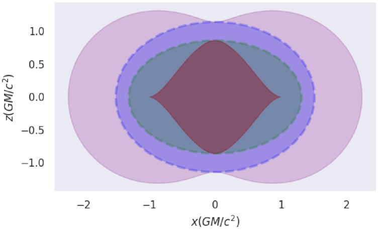
Figure 13: Kerr metric 2D slice in the x-z plane ($y=0$) for a spin parameter $a=0.99$. The following regions plotted are: i) inner ergosphere $r^{\text{ergo}}_{-}$: red region, ii) inner event-horizon $r_{-}$: green region, iii) outer event-horizon $r_{+}$: blue region and iv) outer Ergosphere $r^{\text{ergo}}_{+}$: purple region.

B.2.2 Kretschmann scalar associated with Kerr solution

The nontrivial part of the Kretschmann invariant for the Kerr metric reads:

$$R_{\alpha\beta\gamma\delta}R^{\alpha\beta\gamma\delta}=C_{\alpha\beta\gamma\delta}C^{\alpha\beta\gamma\delta}=\frac{48M^{2}(r^{2}-a^{2}\text{cos}^{2}\vartheta)\big{[}(r^{2}+a^{2}\text{cos}^{2}\vartheta)^{2}-16r^{2}a^{2}\text{cos}^{2}\vartheta\big{]}}{(r^{2}+a^{2}\text{cos}^{2}\vartheta)^{6}}\ .$$ (99)

This guarantees that the curvature singularity ($\mathscr{K}\rightarrow\infty$) occurs at the ring $\Sigma\equiv r^{2}+a^{2}\text{cos}^{2}\vartheta=0$, with zeros at:

$$r=0\ ,\text{and},\ \vartheta=\dfrac{\pi}{2}\ .$$

B.3 Gravitational waves

Linearized gravity models the metric as tiny fluctuations or perturbations $h_{\alpha\beta}$ of the flat background metric $\eta_{\alpha\beta}$:

$$g_{\alpha\beta}\approx\eta_{\alpha\beta}+h_{\alpha\beta}+\mathcal{O}(h_{\alpha\beta})^{2}\ ,$$

where $|h_{\alpha\beta}|\ll 1$. To describe gravitational wave propagation, it is often convenient to reduce the linearized field equations into a simplified form via two gauge fixing conditions, namely, a) harmonic gauge, and b) transverse-traceless (TT) gauge. Thus, the Einstein field equations for gravitational waves assume a succinct wave equation type form:

$$\Box\overline{h}^{(\epsilon)}_{\alpha\beta}=-16\pi T_{\alpha\beta}\ .$$

Here, $\overline{h}^{(\epsilon)}_{\alpha\beta}=h^{(\epsilon)}_{\alpha\beta}-\frac{1}{2}h^{(\epsilon)}\eta_{\alpha\beta}$ and $\Box\equiv\eta^{\alpha\beta}\partial_{\alpha}\partial_{\beta}$ is the d’Alembert operator (wave operator). It can be shown that the PDEs in Equation (B.3) produce gravitational wave solutions.

The transverse-traceless (TT) perturbation (we drop the superscript $(\epsilon)$ for the sake of ease) satisfies the following conditions:

Transverse: $\partial_{\beta}h^{\mathrm{TT}\,\alpha\beta}=0$, i.e., wave propagates perpendicular to perturbation direction,

Traceless: $h^{\mathrm{TT}\,\alpha}_{\ \ \ \alpha}=0$,

Purely spatial: $h_{0\alpha}^{\mathrm{TT}}=0$, i.e., no time components.

Thus, a gravitational wave propagating in the $z$-direction with frequency $\omega$ is given in the TT gauge as:

$$h^{\text{TT}}_{\alpha\beta}=\begin{pmatrix}0&0&0&0\\[10.0pt] 0&h_{+}&h_{\times}&0\\[10.0pt] 0&h_{\times}&h_{+}&0\\[10.0pt] 0&0&0&0\end{pmatrix}\text{cos}\big{(}\omega(t-z)\big{)}\ .$$ (100)

$h_{+}$ and $h_{\times}$ are the amplitudes of the “$+$” (plus) polarization and “$\times$” (cross) polarization.

The complete metric tensor in the linearized gravity setting is given by:

$$g_{\alpha\beta}=\eta_{\alpha\beta}+h^{\text{TT}}_{\alpha\beta}=\begin{pmatrix}-1&0&0&0\\[10.0pt] 0&1+h_{+}\cos\big{(}\omega(t-z)\big{)}&h_{\times}\cos\big{(}\omega(t-z)\big{)}&0\\[10.0pt] 0&h_{\times}\cos\big{(}\omega(t-z)\big{)}&1+h_{+}\cos\big{(}\omega(t-z)\big{)}&0\\[10.0pt] 0&0&0&1\end{pmatrix}\ .$$ (101)

The corresponding line-element in the linearized gravity setting reads:

$$ds^{2} =-dt^{2}+\left[1+h_{+}\cos(\omega(t-z)\big{)}\right]dx^{2}+\left[1-h_{+}\cos(\omega(t-z)\big{)}\right]dy^{2}$$

$$+2h_{\times}\cos(\omega(t-z)\big{)}\,dx\,dy$$ (102)

B.3.0.1 Spin-weighted spherical harmonics (SWSH) metric representation.

We start from the decomposition of the complex gravitational wave strain with the spherical harmonic basis-set expansion (Newman & Penrose, 1962). With the expansion in mode weights $h^{lm}(t,r)$, one can ignore (remove) the angular dependence:

$$h(t,r,\theta,\phi)=h_{+}(t,r,\theta,\phi)-ih_{\times}(t,r,\theta,\phi)=\dfrac{M}{r}\sum_{\ell=|s|}^{\infty}\sum_{|m|\leq\ell}^{\ell}h^{\ell m}(t)\,{}_{-2}Y_{\ell m}(\theta,\phi)\ ,$$ (103)

where, $h(t,r,\theta,\phi)=h_{+}(t,r,\theta,\phi)-ih_{\times}(t,r,\theta,\phi)$ is the complex strain. Thus, for each orbital and azimuthal indices $(\ell,m)$, one can extract the mode $h^{\ell m}(t)$ at a fixed radius $r$, one uses the orthogonality of the spin-weighted spherical harmonics (SWSHs) elements:

$$\dfrac{r}{M}h^{\ell m}(t)=\int_{0}^{2\pi}\int_{0}^{\pi}h(t,r,\theta,\phi)\,{}_{-2}\bar{Y}_{\ell m}(\theta,\phi)\,d\Omega$$ (104)

where, $d\Omega=\sin\theta\,d\theta\,d\phi$ is the spherical volume element and ${}_{-2}\bar{Y}_{\ell m}$ denotes the complex conjugate of the $s=2-n=-2$ where ($n=4$ for $\Psi_{4}$) spin-weighted spherical harmonics. One typically carries out the integral over the 2-sphere $\mathbb{S}^{2}$ numerically on a finite angular grid.

The general formula for SWSHs is:

$${}_{s}Y_{\ell m}(\theta,\phi)=(-1)^{l+m-s}\left[\frac{2\ell+1}{4\pi}\frac{(\ell+m)!(\ell-m)!}{(\ell+s)!(\ell-s)!}\right]^{1/2}\sin^{2\ell}\left(\frac{\theta}{2}\right)e^{im\phi}$$ (105)

$$\sum_{r=0}^{\ell-s}(-1)^{r}\binom{\ell-s}{r}\binom{\ell+s}{r+s-m}\cot^{2r+s-m}\left(\frac{\theta}{2}\right).$$

where the parameters $\ell,m$ are the familiar Laplace spherical harmonics (orbital-angular momentum and azimuthal indices), while $s$ is the additional spin-weight introduced by some underlying gauge group such as $U(1)$. We especially plot for the integers $s=-2,l=m=2$, since they are relevant for GWs and are depicted in Figure 14.

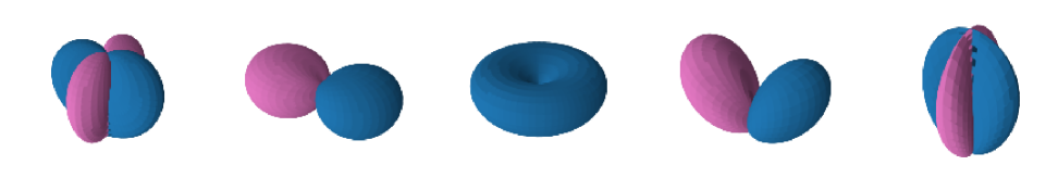
Figure 14: Spin weighted spherical harmonics for $s=-2$, and $l=2$ for $|m|\leq l$. The dominant contributions for the Weyl scalar $\Psi_{4}$ and the associated metric coefficients in the spherical harmonic basis $h^{2,\pm 2}(t)$ are shown.

B.4 Minkowksi metric

B.4.1 Coordinate systems for Minkowski metric

The flat Minkowski metric, which is a spacetime that has no curvature ($M\rightarrow 0)$ can be expressed in other coordinate systems as well.

B.4.1.1 Spherical polar coordinates.

In spherical coordinates $(t,r,\vartheta,\varphi)$, the Minkowski metric is described by the quadratic line element,

$$ds^{2}=-c^{2}dt^{2}+dr^{2}+r^{2}(d\theta^{2}+\text{sin}^{2}d\phi^{2})$$ (106)

here, $r\in\mathbb{R}^{+}$, $\theta\in(0,\pi)$, and, $\phi\in[0,2\pi)$ are the usual spherical polar coordinates. Thus, the metric tensor describing the Schwarzschild solution reads:

$$\eta^{\text{Sph}}_{\mu\nu}=\begin{pmatrix}-1&0&0&0\\ 0&1&0&0\\ 0&0&r^{2}&0\\ 0&0&0&r^{2}\text{sin}^{2}\theta\end{pmatrix}$$ (107)

B.4.1.2 Boyer-Lindquist coordinates.

Setting $M\rightarrow 0$ in the Boyer-Lindquist form of the Kerr metric (94), the corresponding line element reduces to an unfamiliar “oblate-spheroidal" represtation:

$$ds^{2}=-dt^{2}+\frac{r^{2}+a^{2}\text{cos}^{2}\vartheta}{r^{2}+a^{2}}\ dr^{2}+(r^{2}+a^{2}\text{cos}^{2}\vartheta)\ d\vartheta^{2}+(r^{2}+a^{2})\ \text{sin}^{2}\vartheta\ d\phi^{2}\ ,$$ (108)

and the components of the

$$\eta^{\text{BL}}_{\mu\nu}=\begin{pmatrix}-1&0&0&0\\ 0&\frac{r^{2}+a^{2}\text{cos}^{2}\vartheta}{r^{2}+a^{2}}&0&0\\ 0&0&r^{2}+a^{2}\text{cos}^{2}\vartheta&0\\ 0&0&0&(r^{2}+a^{2})\ \text{sin}^{2}\vartheta\end{pmatrix}\ .$$ (109)

The usual Cartesian coordinates can be related to the oblate spheroid ones via:

$$x =\sqrt{r^{2}+a^{2}}\ \text{sin}\ \vartheta\ \text{cos}\ \phi$$

$$y =\sqrt{r^{2}+a^{2}}\ \text{sin}\ \vartheta\ \text{sin}\ \phi$$

$$z =r\ \text{cos}\ \vartheta\ .$$

B.4.1.3 Eddington-Finkelstein coordinates.

The Minkowski metric can be written in the ingoing (advanced) Eddington-Finkelstein form in two different cases, namely for the non-rotating and the rotating case.

• i) non-rotating, $a\rightarrow 0$ (Schwarzschild): :

  $$ds^{2}=-dv^{2}+2\ dv\ dr+r^{2}(d\theta^{2}+\text{sin}^{2}\vartheta\ d\phi^{2})\ ,$$

  and the metric tensor reads:

  $$\eta^{\text{EF}}_{\mu\nu}=\begin{pmatrix}-1&1&0&0\\ 1&0&0&0\\ 0&0&r^{2}&0\\ 0&0&0&r^{2}\ \text{sin}^{2}\theta\end{pmatrix}\ .$$ (110)

• ii) rotating: $a>0$ (Kerr):

  $$ds^{2} =-(dv+a\ \text{sin}^{2}\vartheta d\phi)^{2}+2(dv+a\ \text{sin}^{2}\vartheta d\phi)(dr+a\text{sin}^{2}\vartheta d\phi)$$

  $$+(r^{2}+a^{2}\ \text{cos}^{2}\vartheta)(d\theta^{2}+\text{sin}^{2}d\phi^{2})\ ,$$ (111)

  and the metric tensor reads:

  $$\eta^{\text{EF}}_{\mu\nu}=\begin{pmatrix}-1&1&0&0\\ 1&0&0&a\text{sin}^{2}\vartheta\\ 0&0&\Sigma&0\\ 0&a\text{sin}^{2}\vartheta&0&(r^{2}+a^{2})\ \text{sin}^{2}\vartheta\end{pmatrix}\ .$$ (112)

B.5 Training on non-trivial metric fields (distortions)

Distortion part of Schwarzschild geometry in spherical coordinates:

• Spherical coordinates: obtained by subtracting (107) from (85):

  $$g^{\text{Sph}}_{\mu\nu}-\eta^{\text{Sph}}_{\mu\nu}=\begin{pmatrix}\dfrac{r_{s}}{r}&0&0&0\\[10.0pt] 0&\dfrac{r_{s}}{(r-r_{s})}&0&0\\[10.0pt] 0&0&0&0\\[10.0pt] 0&0&0&0\ \end{pmatrix}\ .$$ (113)

• Kerr-Schild coordinates obtained by subtracting $\eta_{\mu\nu}=\text{diag}(-1,+1,+1,+1)$ from (89):

  $$g^{\text{KS}}_{\mu\nu}-\eta_{\mu\nu}=\begin{pmatrix}\dfrac{2M}{r}&\dfrac{2Mx}{r^{2}}&\dfrac{2My}{r^{2}}&\dfrac{2Mz}{r^{2}}\\[10.0pt] \dfrac{2Mx}{r^{2}}&\dfrac{2Mx^{2}}{r^{3}}&\dfrac{2Mxy}{r^{3}}&\dfrac{2Mxz}{r^{3}}\\[10.0pt] \dfrac{2My}{r^{2}}&\dfrac{2Mxy}{r^{3}}&\dfrac{2My^{2}}{r^{3}}&\dfrac{2Myz}{r^{3}}\\[10.0pt] \dfrac{2Mz}{r^{2}}&\dfrac{2Mxz}{r^{3}}&\dfrac{2Myz}{r^{3}}&\dfrac{2Mz^{2}}{r^{3}}\end{pmatrix}\ .$$ (114)

• Ingoing Eddington-Finkelstein coordinates obtained by subtracting (110) from (92):

  $$g^{\text{EF}}_{\mu\nu}-\eta^{\text{EF}}_{\mu\nu}=\begin{pmatrix}\dfrac{r_{s}}{r}&0&0&0\\[10.0pt] 0&0&0&0\\[10.0pt] 0&0&0&0\\[10.0pt] 0&0&0&0\end{pmatrix}\ .$$ (115)

Distortion part of Kerr geometry:

• Boyer-Lindquist coordinates: obtained by subtracting (109) from (95):

  $$g^{\text{BL}}_{\mu\nu}-\eta^{\text{BL}}_{\mu\nu}=\begin{pmatrix}\dfrac{2Mr}{\Sigma}&0&0&\dfrac{2Mar\sin^{2}\theta}{\Sigma}\\[10.0pt] 0&\dfrac{2M\Sigma}{r\Delta}&0&0\\[10.0pt] 0&0&0&0\\[10.0pt] \dfrac{2Mar\sin^{2}\theta}{\Sigma}&0&0&\dfrac{2Ma^{2}r\sin^{4}\vartheta}{\Sigma}\ \end{pmatrix}\ .$$ (116)

• Kerr-Schild coordinates: obtained by subtracting $\eta=\text{diag }(-1,+1,+1,+1)$ from Equation (96):

• Eddington-Finkelstein coordinates: obtained by subtracting (112) from (98):

  $$g^{\text{EF}}_{\mu\nu}-\eta^{\text{EF}}_{\mu\nu}=\begin{pmatrix}\dfrac{2Mr}{\Sigma}&0&0&\dfrac{2Mar\sin^{2}\theta}{\Sigma}\\[10.0pt] 0&0&0&0\\[10.0pt] 0&0&0&0\\[10.0pt] \dfrac{2Mar\sin^{2}\theta}{\Sigma}&0&0&\dfrac{2Ma^{2}r\sin^{4}\vartheta}{\Sigma}\ \end{pmatrix}\ .$$ (117)

Appendix C Finite-Difference Method (FDM) for Tensor Differentiation

The main concept in this appendix section details numerical differentiation methods for tensor-valued quantities, focusing on the practical use of higher-order finite-difference schemes (in particular, sixth-order stencils). We outline the treatment of discretization errors and the use of neighboring grid collocation points as part of a numerical tensor calculus toolbox.

To compare the performance against automatic differentiation on tensor fields defined on the four dimensional spacetime, throughout the paper we opt for the highly accurate sixth-order order forward difference ($n=6$ accuracy). This scheme queries six neighboring points per evaluation and the general formula of the differential operators are given by:

$$\big{[}\partial_{x^{i}}f(\mathbf{x})\big{]} \approx-\frac{49}{20h}f(\mathbf{x})+\frac{6}{h}f(\mathbf{x+h})-\frac{15}{2h}f(\mathbf{x+2h})+\frac{20}{3h}f(\mathbf{x+3h})$$

$$-\frac{15}{4h}f(\mathbf{x+4h})+\frac{6}{5h}f(\mathbf{x+5h})-\frac{1}{6h}f(\mathbf{x+6h})+\mathcal{O}(\mathbf{h}^{7})$$ (118)

Here, $\mathbf{x}=(x_{1},...,x_{d})\in\mathbb{R}^{d}$ and the $\mathbf{h}=h\mathbf{e}_{i},\ \text{s.t.}\ \mathbf{e}_{i}=(0,..,\underbrace{h}^{\text{i-th index}},..,0)$, depending with respect to the variable $x_{i}$ the partial derivative is performed over. Thus, this is accurate upto $\mathcal{O}(\bm{h}^{6})$, and the truncation error occurs at seventh-order.

In general, for an $n$-th order finite-difference approximation, the stencil is constructed by querying $n$ neighboring collocation points on the voxel grid. The resulting truncation error on function evaluated on the grid (gridfunctions) scales as follows (Ruchlin et al., 2018):

$$\mathscr{E}^{n}_{\text{FD}}[f]=\mathcal{O}\big{(}h^{n}|\partial^{n+1}_{\mathbf{x}}f|\big{)}\ .$$

Thus, higher order stencils enable larger step size $h$ choices since the error scales exponential to the stencil order, i.e, $\mathscr{E}\propto h^{n}$. This results in not only better accuracy, but also lesser memory consumption due to lower grid resolution.

C.0.0.1 Finite-difference method bottlenecks in NR

• Higher-order finite-difference stencils require a collection of padded grid points exterior to the cube as boundary handling. These are often called ghost cells (zones). For e.g., if $n_{g}$ ghost cells are required for the $n$-th order forward difference stencil, the grid size increases of a 3D spatial voxel grid (Ruchlin et al., 2018) $\mathtt{N}_{x}\times\mathtt{N}_{y}\times\mathtt{N}_{z}\rightarrow(\mathtt{N}_{x}+n_{g})\times(\mathtt{N}_{y}+n_{g})\times(\mathtt{N}_{z}+n_{g})$.

• Sensitive to numerical noise especially for tensor-valued functions defined on multidimensional voxel grids.

C.0.0.2 Comparing AD vs FD based methods.

We quantify the performance of automatic-differentiation operations on the ground truth metric against the $6$-th order finite difference stencils. We test it against the Kretschmann scalar $\mathscr{K}=R_{\alpha\beta\gamma\delta}R^{\alpha\beta\gamma\delta}$, which is prone to errors, especially due to floating point errors accumulated in the Riemann curvature tensor:

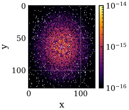
Figure 15: Absolute error $|\mathscr{K}_{\text{analytic}}-\mathscr{K}_{\text{AD}}|$ profile plotted for $z=0.3$ between the analytic Kretschmann scalar and the ground truth Kretschmann scalar obtained via AD implemented on the ground truth (analytic) metric.

Appendix D Experimental details

This appendix provides detailed experimental specifics, including: (i) gradient alignment aspects relevant to SOAP optimizers; (ii) error plots for the metric and higher-rank differential geometric quantities, with component-wise tomography where applicable; (iii) training across varied coordinate systems to illustrate the coordinate-choice flexibility of NeFs; (iv) the hyperparameter configurations employed; and (v) the hardware and software environments used for these experiments.

D.1 Gradient alignment

Competing tasks is a well-known problem in multi-objective learning (Yu et al. (2020), Liu et al. (2021), Shi et al. (2023)), the gradients of the loss functions pull the weights in different directions. In Scientific Machine Learning (SciML), a lot of work emerged in analyzing and mitigating gradient conflicts in the context of PINNs (Wang et al. (2025), Lui et al. (2025), Hwang & Lim (2025)). Although Sobolev training differs from PINNs, particularly from a supervision perspective, it exhibits the same problem where some loss terms dominate others. In PINNs, the training is highly dependent on first satisfying the initial/boundary conditions, which provide uniqueness to the solution. The different levels of complexity between these and the residual loss create different optimization priorities, but both losses are equally important. Similarly, Sobolev training faces analogous challenges with competing loss components. The Jacobian data serve to constrain the model’s derivatives, while the target function outputs determine the integration "constant", both components being equally valuable. However, the sources of complexity differ between these approaches. In PINNs, the primary challenge stems from determining a solution through unsupervised learning on PDE losses, whereas in our Sobolev training specifically, the complexity arises from managing optimization stability in high-dimensional spaces: a $\mathtt{16}$-dimensional output space, $\mathtt{64}$-dimensional Jacobian, and $\mathtt{256}$-dimensional Hessian. Moreover, this complexity is accompanied by the challenge of handling gradient imbalances. Depending on the point in spacetime, the metric or its derivatives dominate in the loss. Generally speaking, an analogy is to think $g_{\mu\nu}\propto\frac{1}{r}$,$\partial_{\rho}g_{\mu\nu}\propto\frac{1}{r^{2}}$ and $\partial_{\sigma\rho}g_{\mu\nu}\propto\frac{1}{r^{3}}$, making it clear how gradient magnitudes differ depending on the radius.

Mitigating gradient conflicts does not necessarily result in better accuracy, but it explains a possible reason why the loss does not improve further, the optimization being stuck in the local minimum of one of the objectives. The intra-step gradient alignment scores presented in Wang et al. (2025) demonstrate SOAP as a far superior alternative compared to other well-established optimizers, or at least for the experiments considered in that study. To provide a direct comparison using the same methodology as in Wang et al. (2025), we evaluated both ADAM and SOAP on the Cartesian KS representation of the Kerr metric, chosen as the most complex metric investigated in this work. The Sobolev training contains only two objectives: metric and Jacobian supervision. For our experimental setup, we employed an MLP architecture with $\mathtt{5}$ hidden layers, $\mathtt{190}$ hidden units per layer, and SILU activation function to compare gradient conflicts between the two optimizers. The training utilized a cosine decay learning rate schedule, starting from an initial learning rate of $\mathtt{1E{-2}}$ and decaying to a final rate of $\mathtt{1E{-8}}$ over $\mathtt{200}$ epochs. For weighting the losses, gradient normalization was used with and without an exponential moving average. As shown in Figure 15, even though Adam is providing twice as much gradient alignment score in almost all epochs, SOAP’s second-order and preconditioning capabilities allow for a 100x training loss improvement.

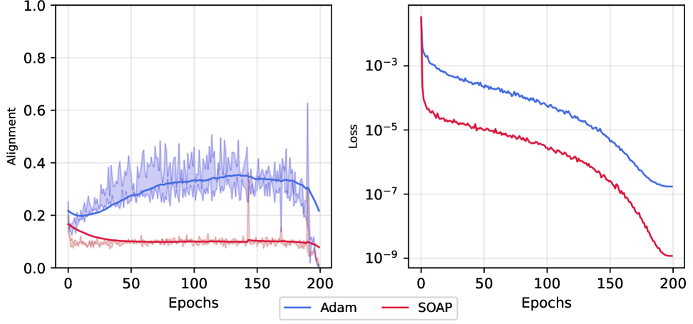
Figure 16: Average gradient alignment per epoch (left) and MSE loss during training for Adam and Soap optimizers (right). The shaded light color in the alignment plot represents a minimum and maximum deviation compared to using an exponential moving average or not for the weights multiplying the gradients.

D.2 Kerr metric error visualization

To quantify the quality of EinFields parametrized metric tensor fields for the Kerr metric with spin parameter $a=0.7$, we report the mean absolute error (MAE) between the ground truth and the NeF-fitted metric tensors in Figure 17. The evaluation is performed on a validation grid with collocation points sampled arbitrarily within the training range but distinct from the training collocation points. Using a model configured with SiLU activations, SOAP optimizer, GradNorm, and without Sobolev regularization, we observe agreement with the ground truth up to six decimal places, achieving an MAE on the order of $\mathtt{1E{-6}}$.

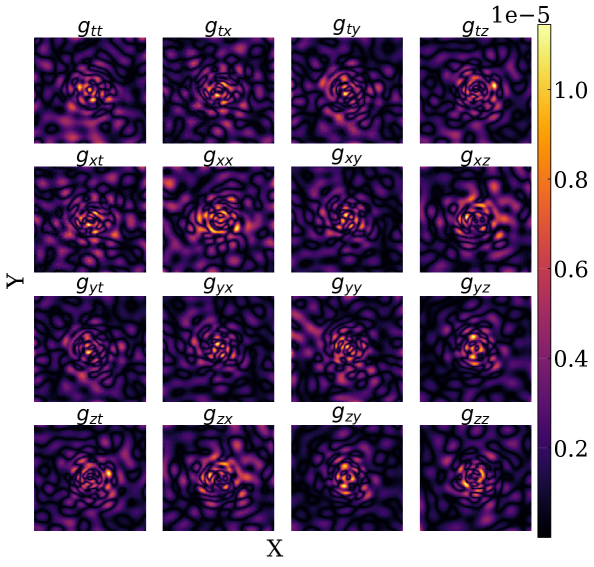
Figure 17: Kerr metric absolute error between ground truth (analytic) metric and the EinFields parametrized metric. The metrics are depicted in the Cartesian Kerr-Schild (KS) representation as presented in Equation (96). The 2D slice of all the metric components captured in the x-y plane at fixed $z=1.4$ for a spin parameter value $a=0.7$.

D.3 Tomography: Metric, metric Jacobian and metric Hessian components

The effect of introducing losses pertaining to metric Jacobian and Hessian supervision, apart from the metric loss that EinFields predominantly uses, can be quantified and visualized with the following plots below. Here, for the sake of visualization, we do a tomography (2D cuts) of different metric components along a particular axis for the Kerr metric in Cartesian KS coordinates (Equation (96)).

The first, second, and third columns in each figure correspond to EinFields training without Sobolev supervision, EinFields (+Jac), and EinFields (+Jac + Hess) trained, respectively, for randomly sampled components of differential geometric quantities.

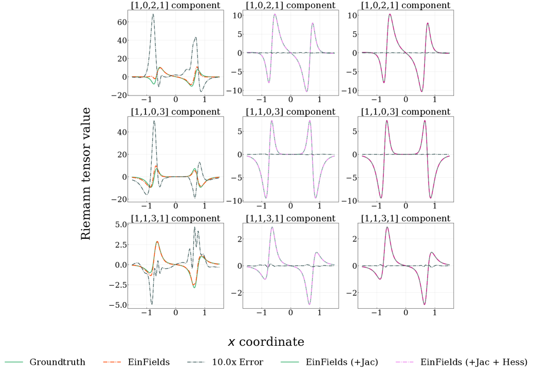
Figure 18: 2D Tomography of Kerr Riemann tensor components in Cartesian KS representation.

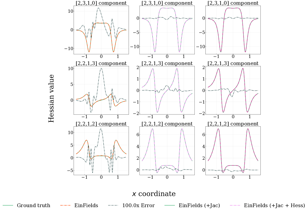
Figure 21: 2D Tomography of Kerr metric Hessian components in Cartesian KS representation.

Figure 22: 2D Tomography of Kerr Christoffel symbols components in Cartesian KS representation.

D.4 Training on varied coordinate systems

NeFs take physical coordinates as inputs and map them directly to field values. Unlike traditional machine learning architectures that ingest abstract learned feature spaces (such as token embeddings or extracted features), INRs operate directly on the physical coordinate space, enabling them to represent continuous signals in a domain-agnostic manner.

In the context of GR, this implies that a four-dimensional representation of metric tensor fields by an INR explicitly depends on the input coordinate system, or more generally, on the chosen frame of reference. Despite this apparent dependency, GR possesses the fundamental property of diffeomorphism covariance (see Section A.3.8), which asserts that the laws of gravitation remain invariant under smooth coordinate transformations. However, the choice of coordinate system remains an essential practical tool for simplifying the form of the metric tensor. For example, while the Schwarzschild metric is diagonal in spherical coordinates (albeit with a coordinate singularity at the event horizon), transforming to Cartesian KS coordinates produces a dense, off-diagonal metric representation, or, for that matter, moving to Eddington-Finkelstein coordinates, which both remove coordinate-related artifacts (see Paragraph A.3.5.5).

Understanding this behavior is essential for developing robust INR-based frameworks for representing geometric quantities in numerical relativity, while respecting the underlying diffeomorphism invariance of general relativity.

For the Schwarzschild case, we initiate the training by sampling query spacetime coordinates in spherical representation $(t,r,\theta,\phi)$. These sampled collocation points are then transformed into their corresponding collocation points in Cartesian coordinates $(t,x,y,z)$ and ingoing Eddington-Finkelstein coordinates $(v,r,\theta,\tilde{\phi})$ (see Section B.1.1 for explicit transformation details). Subsequently, EinFields outputs the metric tensors corresponding to these coordinate systems, yielding Equations ((85), (89), (92)).

For the Kerr metric, which is characterized by its oblate spheroidal geometry, we sample query collocation points in the Boyer-Lindquist coordinates $(t,r,\vartheta,\phi)$, followed by the collocation points transformed into Cartesian $(t,x,y,z)$ and ingoing Eddington-Finkelstein coordinates $(t,r,\theta,\tilde{\phi})$. EinFields then outputs the Kerr metric tensors in these respective coordinate systems, resulting in Equations ((95), (96), (98)).

This multi coordinate training strategy ensures that the neural tensor field learns consistent representations across coordinate systems while maintaining geometric and physical consistency under diffeomorphisms, facilitating generalization and stability in downstream geometric learning tasks.

Metric	Representation	Coordinate	Rel. L2
Schwarzschild	EinFields	Spherical	2.26E-7
		Cartesian Kerr-Schild	1.37E-5
		Eddington-Finkelstein	9.21E-9
	EinFields (+ Jac)	Spherical	1.37E-7
		Cartesian Kerr-Schild	3.00E-6
		Eddington-Finkelstein	6.47E-9
	EinFields (+ Jac + Hess)	Spherical	1.20E-7
		Cartesian Kerr-Schild	1.53E-6
		Eddington-Finkelstein	9.08E-9
Kerr	EinFields	Boyer-Lindquist	6.95E-8
		Cartesian Kerr-Schild	4.47E-6
		Eddington-Finkelstein	6.44E-8
	EinFields (+ Jac)	Boyer-Lindquist	4.72E-8
		Cartesian Kerr-Schild	8.83E-7
		Eddington-Finkelstein	4.95E-8
	EinFields (+ Jac + Hess)	Boyer-Lindquist	4.69E-8
		Cartesian Kerr-Schild	4.95E-7
		Eddington-Finkelstein	4.72E-8

Table 9: Relative L2 error considered on a grid of validation collocation points (i) EinFields, (ii) EinFields (+Jac) and, (iii) EinFields (+Jac + Hess) supervision. As described above in the text, we quantify the effect of inputs queries in varied coordinate charts and how EinFields training generalizes over these different metric (geometry) representations.

D.5 Training hyperparameters

Table 10: Training configurations for Schwarzschild, Kerr, and GWs used in the geodesics, Kretschmann plots, Table 8, and linearized gravity section.

Parameter	Schwarzschild	Kerr	GWs
Architecture	MLP
Depth	3 / 3 / 5 / 7	5	5
Width	64 / 128 / 256 / 512	190	128 / 128 / 90
Activation	SiLU	SiLU	SiLU / SIREN / WIRE
Input dimension	4	4	4
Output dimension	10 / 16	16	16
# Parameters	13.5K / 50K / 332K / 1.5M	185K	85K
Optimizer	SOAP
$\beta_{1}$	0.95
$\beta_{2}$	0.95
Precondition frequency	1
Learning rate schedule
Initial learning rate	E-2 / E-3
Decay steps	$10^{4}$	$6\times 10^{3}$ / $2,4,6\ \times 10^{4}$	$4\times 10^{3}$ / $4\times 10^{4}$
Final learning rate	E-5 / E-6	E-7 / E-8	E-9
Training
Epochs	100	200	200
Number of batches	100	30 / 100 / 200 / 300	20 / 200
Gradient weighting scheme	None / GradNorm

D.6 Hardware

For our primary computational work, we utilize a high-performance CPU system equipped with 2×32-core Intel® Xeon® Platinum 8452Y+ processors, each operating at 4.1 GHz, and 2048 GiB of RAM. All NeF-related training is performed on a single NVIDIA H200 SXM GPU with 144 GiB of HBM3e memory. For prototyping and preliminary experiments, we employ a single NVIDIA Tesla A100 GPU with 40 GiB of memory.

Appendix E Licenses

This work would not have been possible without the open-source software ecosystem. Our implementation is built upon multiple community-maintained libraries, and we gratefully acknowledge their licenses below. The core computations were performed using JAX[cuda12] (Bradbury et al., 2018) with CUDA support, licensed under the Apache 2.0 License. For model definition and training, we relied on Equinox (Kidger & Garcia, 2021) and Flax.Linen (Heek et al., 2024), both also under Apache 2.0. For solving differential equations, we employed Diffrax (Kidger, 2021), distributed under the Apache 2.0 License. All libraries used are permissively licensed, enabling free academic and non-commercial research.

References

- Abac et al. (2025) Adrian Abac et al. The science of the einstein telescope, 2025.
- Abbott et al. (2016a) B. P. Abbott et al. Observation of gravitational waves from a binary black hole merger. Phys. Rev. Lett., 116:061102, Feb 2016a. doi: 10.1103/PhysRevLett.116.061102.
- Abbott et al. (2016b) B. P. Abbott et al. Gw150914: The advanced ligo detectors in the era of first discoveries. Phys. Rev. Lett., 116:131103, Mar 2016b. doi: 10.1103/PhysRevLett.116.131103.
- Abbott et al. (2016c) B. P. Abbott et al. Properties of the binary black hole merger gw150914. Phys. Rev. Lett., 116:241102, Jun 2016c. doi: 10.1103/PhysRevLett.116.241102.
- Abbott et al. (2017) B. P. Abbott et al. Multi-messenger observations of a binary neutron star merger*. The Astrophysical Journal Letters, 848(2):L12, oct 2017. doi: 10.3847/2041-8213/aa91c9.
- Acernese et al. (2014) F Acernese et al. Advanced virgo: a second-generation interferometric gravitational wave detector. Classical and Quantum Gravity, 32(2):024001, dec 2014. doi: 10.1088/0264-9381/32/2/024001.
- Amaro-Seoane et al. (2017) Pau Amaro-Seoane et al. Laser interferometer space antenna, 2017.
- Arnowitt et al. (1959) R. Arnowitt, S. Deser, and C. W. Misner. Dynamical structure and definition of energy in general relativity. Phys. Rev., 116:1322–1330, Dec 1959. doi: 10.1103/PhysRev.116.1322.
- Baydin et al. (2018) Atilim Gunes Baydin, Barak A. Pearlmutter, Alexey Andreyevich Radul, and Jeffrey Mark Siskind. Automatic differentiation in machine learning: a survey, 2018.
- Behler & Parrinello (2007) Jörg Behler and Michele Parrinello. Generalized neural-network representation of high-dimensional potential-energy surfaces. Phys. Rev. Lett., 98:146401, Apr 2007. doi: 10.1103/PhysRevLett.98.146401.
- Berger & Oliger (1984) Marsha J Berger and Joseph Oliger. Adaptive mesh refinement for hyperbolic partial differential equations. Journal of Computational Physics, 53(3):484–512, 1984. ISSN 0021-9991. doi: https://doi.org/10.1016/0021-9991(84)90073-1.
- Berzins et al. (2025) Arturs Berzins, Andreas Radler, Eric Volkmann, Sebastian Sanokowski, Sepp Hochreiter, and Johannes Brandstetter. Geometry-informed neural networks. In Forty-second International Conference on Machine Learning, 2025.
- Birkhoff & Langer (1923) G.D. Birkhoff and R.E. Langer. Relativity and Modern Physics. Harvard University Press, 1923.
- Bodnar et al. (2025) Cristian Bodnar, Wessel P Bruinsma, Ana Lucic, Megan Stanley, Anna Allen, Johannes Brandstetter, Patrick Garvan, Maik Riechert, Jonathan A Weyn, Haiyu Dong, Jayesh K Gupta, Kit Thambiratnam, Alexander T Archibald, Chun-Chieh Wu, Elizabeth Heider, Max Welling, Richard E Turner, and Paris Perdikaris. A foundation model for the earth system. Nature, 641(8065):1180–1187, May 2025.
- Bott & Tu (1982) Raoul Bott and Loring W. Tu. de Rham Theory, pp. 13–88. Springer New York, New York, NY, 1982. ISBN 978-1-4757-3951-0. doi: 10.1007/978-1-4757-3951-0_2.
- Boyer & Lindquist (1967) Robert H. Boyer and Richard W. Lindquist. Maximal analytic extension of the kerr metric. Journal of Mathematical Physics, 8(2):265–281, 02 1967. ISSN 0022-2488. doi: 10.1063/1.1705193.
- Boyle et al. (2025) Michael Boyle, Keefe Mitman, Mark Scheel, and Leo Stein. The sxs package, May 2025.
- Boyle et al. (2019) Michael Boyle et al. The sxs collaboration catalog of binary black hole simulations. Classical and Quantum Gravity, 36(19):195006, sep 2019. doi: 10.1088/1361-6382/ab34e2.
- Bradbury et al. (2018) James Bradbury, Roy Frostig, Peter Hawkins, Matthew James Johnson, Chris Leary, Dougal Maclaurin, George Necula, Adam Paszke, Jake VanderPlas, Skye Wanderman-Milne, and Qiao Zhang. JAX: composable transformations of Python+NumPy programs, 2018.
- Brandstetter (2025) Johannes Brandstetter. Envisioning better benchmarks for machine learning PDE solvers. Nat. Mac. Intell., 7(1):2–3, 2025. doi: 10.1038/S42256-024-00962-Z.
- Brandstetter et al. (2022) Johannes Brandstetter, Daniel E. Worrall, and Max Welling. Message passing neural PDE solvers. In The Tenth International Conference on Learning Representations, ICLR 2022, Virtual Event, April 25-29, 2022. OpenReview.net, 2022.
- Bronstein et al. (2021) Michael M. Bronstein, Joan Bruna, Taco Cohen, and Petar Velickovic. Geometric deep learning: Grids, groups, graphs, geodesics, and gauges. CoRR, abs/2104.13478, 2021.
- Brunton et al. (2020) Steven L Brunton, Bernd R Noack, and Petros Koumoutsakos. Machine learning for fluid mechanics. Annual review of fluid mechanics, 52(1):477–508, 2020.
- Carroll et al. (2004) S. Carroll, S.M. Carroll, and Addison-Wesley. Spacetime and Geometry: An Introduction to General Relativity. Addison Wesley, 2004. ISBN 9780805387322.
- Castelvecchi (2017) Davide Castelvecchi. Gravitational wave detection wins physics nobel. Nature, 550(7674):19–19, October 2017.
- Chandrasekhar (1984) S. Chandrasekhar. The Mathematical Theory of Black Holes, pp. 5–26. Springer Netherlands, Dordrecht, 1984. ISBN 978-94-009-6469-3. doi: 10.1007/978-94-009-6469-3_2.
- Chen et al. (2023) Honglin Chen, Rundi Wu, Eitan Grinspun, Changxi Zheng, and Peter Yichen Chen. Implicit neural spatial representations for time-dependent pdes. In Andreas Krause, Emma Brunskill, Kyunghyun Cho, Barbara Engelhardt, Sivan Sabato, and Jonathan Scarlett (eds.), International Conference on Machine Learning, ICML 2023, 23-29 July 2023, Honolulu, Hawaii, USA, volume 202 of Proceedings of Machine Learning Research, pp. 5162–5177. PMLR, 2023.
- Chen et al. (2018) Zhao Chen, Vijay Badrinarayanan, Chen-Yu Lee, and Andrew Rabinovich. Gradnorm: Gradient normalization for adaptive loss balancing in deep multitask networks. In International conference on machine learning, pp. 794–803. PMLR, 2018.
- Chen & Zhang (2019) Zhiqin Chen and Hao Zhang. Learning implicit fields for generative shape modeling. In Proceedings of the IEEE/CVF Conference on Computer Vision and Pattern Recognition, pp. 5939–5948, 2019.
- Chetan et al. (2024) Aditya Chetan, Guandao Yang, Zichen Wang, Steve Marschner, and Bharath Hariharan. Accurate differential operators for neural fields, 2024.
- Collaboration et al. (2015) The LIGO Scientific Collaboration, Aasi, et al. Advanced ligo. Classical and Quantum Gravity, 32(7):074001, mar 2015. doi: 10.1088/0264-9381/32/7/074001.
- Czarnecki et al. (2017) Wojciech Marian Czarnecki, Simon Osindero, Max Jaderberg, Grzegorz Swirszcz, and Razvan Pascanu. Sobolev training for neural networks. In Proceedings of the 31st International Conference on Neural Information Processing Systems, NIPS’17, pp. 4281–4290, Red Hook, NY, USA, 2017. Curran Associates Inc. ISBN 9781510860964.
- Dean et al. (2012) Jeffrey Dean et al. Large scale distributed deep networks. In Proceedings of the 26th International Conference on Neural Information Processing Systems - Volume 1, NIPS’12, pp. 1223–1231, Red Hook, NY, USA, 2012. Curran Associates Inc.
- Deppe et al. (2025) Nils Deppe, William Throwe, Lawrence E. Kidder, Nils L. Vu, Kyle C. Nelli, Cristóbal Armaza, Marceline S. Bonilla, François Hébert, Yoonsoo Kim, Prayush Kumar, Geoffrey Lovelace, Alexandra Macedo, Jordan Moxon, Eamonn O’Shea, Harald P. Pfeiffer, Mark A. Scheel, Saul A. Teukolsky, Nikolas A. Wittek, et al. SpECTRE v2025.04.21, 4 2025.
- Elfwing et al. (2018) Stefan Elfwing, Eiji Uchibe, and Kenji Doya. Sigmoid-weighted linear units for neural network function approximation in reinforcement learning. Neural Networks, 107:3–11, 2018. doi: 10.1016/J.NEUNET.2017.12.012.
- Essakine et al. (2024) Amer Essakine, Yanqi Cheng, Chun-Wun Cheng, Lipei Zhang, Zhongying Deng, Lei Zhu, Carola-Bibiane Schönlieb, and Angelica I Aviles-Rivero. Where do we stand with implicit neural representations? a technical and performance survey. arXiv preprint arXiv:2411.03688, 2024.
- Everitt et al. (2011) C. W. F. Everitt, D. B. DeBra, B. W. Parkinson, J. P. Turneaure, J. W. Conklin, M. I. Heifetz, G. M. Keiser, A. S. Silbergleit, T. Holmes, J. Kolodziejczak, M. Al-Meshari, J. C. Mester, B. Muhlfelder, V. G. Solomonik, K. Stahl, P. W. Worden, W. Bencze, S. Buchman, B. Clarke, A. Al-Jadaan, H. Al-Jibreen, J. Li, J. A. Lipa, J. M. Lockhart, B. Al-Suwaidan, M. Taber, and S. Wang. Gravity probe b: Final results of a space experiment to test general relativity. Phys. Rev. Lett., 106:221101, May 2011. doi: 10.1103/PhysRevLett.106.221101.
- Fornberg (1996) Bengt Fornberg. Introduction, pp. 1–3. Cambridge Monographs on Applied and Computational Mathematics. Cambridge University Press, 1996.
- Frolov & Novikov (1998) V. Frolov and I. Novikov. Black Hole Physics: Basic Concepts and New Developments. Fundamental Theories of Physics. Springer Netherlands, 1998. ISBN 9780792351450.
- Fuerst, S. V. & Wu, K. (2004) Fuerst, S. V. and Wu, K. Radiation transfer of emission lines in curved space-time*. A&A, 424(3):733–746, 2004. doi: 10.1051/0004-6361:20035814.
- Griewank & Walther (2008) A. Griewank and A. Walther. Evaluating Derivatives: Principles and Techniques of Algorithmic Differentiation, Second Edition. Other Titles in Applied Mathematics. Society for Industrial and Applied Mathematics, 2008. ISBN 9780898716597.
- Griewank (2003) Andreas Griewank. A mathematical view of automatic differentiation. Acta Numerica, 12:321–398, 2003. doi: 10.1017/S0962492902000132.
- Haas et al. (2016) Roland Haas, Christian D. Ott, Bela Szilagyi, Jeffrey D. Kaplan, Jonas Lippuner, Mark A. Scheel, Kevin Barkett, Curran D. Muhlberger, Tim Dietrich, Matthew D. Duez, Francois Foucart, Harald P. Pfeiffer, Lawrence E. Kidder, and Saul A. Teukolsky. Simulations of inspiraling and merging double neutron stars using the spectral einstein code. Phys. Rev. D, 93:124062, Jun 2016. doi: 10.1103/PhysRevD.93.124062.
- Hayashi et al. (2025) Kota Hayashi, Kenta Kiuchi, Koutarou Kyutoku, Yuichiro Sekiguchi, and Masaru Shibata. Jet from binary neutron star merger with prompt black hole formation. Phys. Rev. Lett., 134:211407, May 2025. doi: 10.1103/PhysRevLett.134.211407.
- Heek et al. (2024) Jonathan Heek, Anselm Levskaya, Avital Oliver, Marvin Ritter, Bertrand Rondepierre, Andreas Steiner, and Marc van Zee. Flax: A neural network library and ecosystem for JAX, 2024.
- Hirst et al. (2025) Edward Hirst, Tancredi Schettini Gherardini, and Alexander G. Stapleton. Ainstein: Numerical einstein metrics via machine learning, 2025.
- Hornik et al. (1990) Kurt Hornik, Maxwell Stinchcombe, and Halbert White. Universal approximation of an unknown mapping and its derivatives using multilayer feedforward networks. Neural Networks, 3(5):551–560, 1990. ISSN 0893-6080. doi: https://doi.org/10.1016/0893-6080(90)90005-6.
- Huerta et al. (2019) E. A. Huerta, Roland Haas, Sarah Habib, Anushri Gupta, Adam Rebei, Vishnu Chavva, Daniel Johnson, Shawn Rosofsky, Erik Wessel, Bhanu Agarwal, Diyu Luo, and Wei Ren. Physics of eccentric binary black hole mergers: A numerical relativity perspective. Phys. Rev. D, 100:064003, Sep 2019. doi: 10.1103/PhysRevD.100.064003.
- Hwang & Lim (2025) Youngsik Hwang and Dong-Young Lim. Dual cone gradient descent for training physics-informed neural networks, 2025.
- Isham (1999) C.J. Isham. Modern Differential Geometry for Physicists. World Scientific lecture notes in physics. World Scientific, 1999. ISBN 9789810235628.
- Izzo & Gómez (2022) Dario Izzo and Pablo Gómez. Geodesy of irregular small bodies via neural density fields. Communications Engineering, 1(1):48, December 2022.
- Jost (2008) Jürgen Jost. Riemannian Geometry and Geometric Analysis. Universitext. Springer Berlin, Heidelberg, Berlin, Heidelberg, 5th edition, 2008. ISBN 978-3-540-77341-2. doi: 10.1007/978-3-540-77341-2.
- Karniadakis et al. (2021) George Em Karniadakis, Ioannis G Kevrekidis, Lu Lu, Paris Perdikaris, Sifan Wang, and Liu Yang. Physics-informed machine learning. Nature Reviews Physics, 3(6):422–440, June 2021.
- Karras et al. (2021) Tero Karras, Miika Aittala, Samuli Laine, Erik Härkönen, Janne Hellsten, Jaakko Lehtinen, and Timo Aila. Alias-free generative adversarial networks. In M. Ranzato, A. Beygelzimer, Y. Dauphin, P.S. Liang, and J. Wortman Vaughan (eds.), Advances in Neural Information Processing Systems, volume 34, pp. 852–863. Curran Associates, Inc., 2021.
- Kerr & Schild (2009) R P Kerr and A Schild. Republication of: A new class of vacuum solutions of the einstein field equations. General Relativity and Gravitation, 41(10):2485–2499, October 2009.
- Kidger (2021) Patrick Kidger. On Neural Differential Equations. PhD thesis, University of Oxford, 2021.
- Kidger & Garcia (2021) Patrick Kidger and Cristian Garcia. Equinox: neural networks in JAX via callable PyTrees and filtered transformations. Differentiable Programming workshop at Neural Information Processing Systems 2021, 2021.
- Kingma & Ba (2015) Diederik P. Kingma and Jimmy Ba. Adam: A method for stochastic optimization. In Yoshua Bengio and Yann LeCun (eds.), 3rd International Conference on Learning Representations, ICLR 2015, San Diego, CA, USA, May 7-9, 2015, Conference Track Proceedings, 2015.
- Kobayashi & Nomizu (1963) S. Kobayashi and K. Nomizu. Foundations of Differential Geometry. Number Bd. 1 in Foundations of Differential Geometry. Interscience Publishers, 1963. ISBN 9780470496480.
- Krasiński (1978) Andrzej Krasiński. Ellipsoidal space-times, sources for the kerr metric. Annals of Physics, 112(1):22–40, 1978. ISSN 0003-4916. doi: https://doi.org/10.1016/0003-4916(78)90079-9.
- Kreiss (1994) Heinz-Otto Kreiss. Difference Methods for Time-Dependent Partial Differential Equations, pp. 209–238. Springer New York, New York, NY, 1994. ISBN 978-1-4612-0859-4. doi: 10.1007/978-1-4612-0859-4_7.
- Krishnan et al. (2020) V. Venkatraman Krishnan, M. Bailes, W. van Straten, N. Wex, P. C. C. Freire, E. F. Keane, T. M. Tauris, P. A. Rosado, N. D. R. Bhat, C. Flynn, A. Jameson, and S. Osłowski. Lense–thirring frame dragging induced by a fast-rotating white dwarf in a binary pulsar system. Science, 367(6477):577–580, 2020. doi: 10.1126/science.aax7007.
- Lee (2012) J. Lee. Introduction to Smooth Manifolds. Graduate Texts in Mathematics. Springer New York, 2012. ISBN 9781441999825.
- Li et al. (2023) Zhi-Han Li, Chen-Qi Li, and Long-Gang Pang. Solving einstein equations using deep learning, 2023.
- Li et al. (2021) Zongyi Li, Nikola Borislavov Kovachki, Kamyar Azizzadenesheli, Burigede Liu, Kaushik Bhattacharya, Andrew M. Stuart, and Anima Anandkumar. Fourier neural operator for parametric partial differential equations. In 9th International Conference on Learning Representations, ICLR 2021, Virtual Event, Austria, May 3-7, 2021. OpenReview.net, 2021.
- Lindblom et al. (2006) Lee Lindblom, Mark A Scheel, Lawrence E Kidder, Robert Owen, and Oliver Rinne. A new generalized harmonic evolution system. Classical and Quantum Gravity, 23(16):S447, jul 2006. doi: 10.1088/0264-9381/23/16/S09.
- Liu et al. (2021) Bo Liu, Xingchao Liu, Xiaojie Jin, Peter Stone, and Qiang Liu. Conflict-averse gradient descent for multi-task learning, 2021.
- Lui et al. (2025) Qiang Lui, Mengyu Chu, and Nils Thuerey. Config: Towards conflict-free training of physics informed neural networks, 2025.
- Luna et al. (2023) Raimon Luna, Juan Calderón Bustillo, Juan José Seoane Martínez, Alejandro Torres-Forné, and José A. Font. Solving the teukolsky equation with physics-informed neural networks. Phys. Rev. D, 107:064025, Mar 2023. doi: 10.1103/PhysRevD.107.064025.
- Mescheder et al. (2019) Lars Mescheder, Michael Oechsle, Michael Niemeyer, Sebastian Nowozin, and Andreas Geiger. Occupancy networks: Learning 3d reconstruction in function space. In Proceedings of the IEEE/CVF Conference on Computer Vision and Pattern Recognition, pp. 4460–4470, 2019.
- Mildenhall et al. (2021) Ben Mildenhall, Pratul P Srinivasan, Matthew Tancik, Jonathan T Barron, Ravi Ramamoorthi, and Ren Ng. Nerf: Representing scenes as neural radiance fields for view synthesis. Communications of the ACM, 65(1):99–106, 2021.
- Misner et al. (2017) C.W. Misner, K.S. Thorne, J.A. Wheeler, and D.I. Kaiser. Gravitation. Princeton University Press, 2017. ISBN 9780691177793.
- Müller et al. (2022) Thomas Müller, Alex Evans, Christoph Schied, and Alexander Keller. Instant neural graphics primitives with a multiresolution hash encoding. ACM Transactions on Graphics, 41(4):1–15, July 2022. ISSN 1557-7368. doi: 10.1145/3528223.3530127.
- Newman & Penrose (1962) Ezra Newman and Roger Penrose. An approach to gravitational radiation by a method of spin coefficients. Journal of Mathematical Physics, 3(3):566–578, 05 1962. ISSN 0022-2488. doi: 10.1063/1.1724257.
- Novello et al. (2022) Tiago Novello, Guilherme Schardong, Luiz Schirmer, Vinícius da Silva, Hélio Lopes, and Luiz Velho. Exploring differential geometry in neural implicits. Computers & Graphics, 108:49–60, 2022. ISSN 0097-8493. doi: https://doi.org/10.1016/j.cag.2022.09.003.
- Papa et al. (2024) Samuele Papa, Riccardo Valperga, David Knigge, Miltiadis Kofinas, Phillip Lippe, Jan-Jakob Sonke, and Efstratios Gavves. How to train neural field representations: A comprehensive study and benchmark, 2024.
- Park et al. (2019) Jeong Joon Park, Peter Florence, Julian Straub, Richard Newcombe, and Steven Lovegrove. DeepSDF: Learning continuous signed distance functions for shape representation. In Proceedings of the IEEE/CVF Conference on Computer Vision and Pattern Recognition, pp. 165–174, 2019.
- Poisson (2004) Eric Poisson. A Relativist’s Toolkit: The Mathematics of Black-Hole Mechanics. Cambridge University Press, 2004.
- Punturo et al. (2010) M Punturo et al. The einstein telescope: a third-generation gravitational wave observatory. Classical and Quantum Gravity, 27(19):194002, sep 2010. doi: 10.1088/0264-9381/27/19/194002.
- Raissi et al. (2019) M. Raissi, P. Perdikaris, and G.E. Karniadakis. Physics-informed neural networks: A deep learning framework for solving forward and inverse problems involving nonlinear partial differential equations. Journal of Computational Physics, 378:686–707, 2019. ISSN 0021-9991. doi: https://doi.org/10.1016/j.jcp.2018.10.045.
- Rashti et al. (2025) Alireza Rashti, Rossella Gamba, Koustav Chandra, David Radice, Boris Daszuta, William Cook, and Sebastiano Bernuzzi. Binary black hole waveforms from high-resolution gr-athena++ simulations. Phys. Rev. D, 111:104078, May 2025. doi: 10.1103/n5pz-qv3x.
- Reed et al. (2021) Albert Reed, Thomas Blanford, Daniel C. Brown, and Suren Jayasuriya. Implicit neural representations for deconvolving sas images, 2021.
- Rizzo et al. (2025) Maxwell Rizzo et al. The einstein toolkit, May 2025.
- Ruchlin et al. (2018) Ian Ruchlin, Zachariah B. Etienne, and Thomas W. Baumgarte. : Numerical relativity in singular curvilinear coordinate systems. Phys. Rev. D, 97:064036, Mar 2018. doi: 10.1103/PhysRevD.97.064036.
- Saragadam et al. (2023) Vishwanath Saragadam, Daniel LeJeune, Jasper Tan, Guha Balakrishnan, Ashok Veeraraghavan, and Richard G. Baraniuk. Wire: Wavelet implicit neural representations, 2023.
- Scheel et al. (2025) Mark A. Scheel et al. The sxs collaboration’s third catalog of binary black hole simulations, 2025.
- Shi et al. (2023) Guangyuan Shi, Qimai Li, Wenlong Zhang, Jiaxin Chen, and Xiao-Ming Wu. Recon: Reducing conflicting gradients from the root for multi-task learning, 2023.
- Shibata & Nakamura (1995) Masaru Shibata and Takashi Nakamura. Evolution of three-dimensional gravitational waves: Harmonic slicing case. Phys. Rev. D, 52:5428–5444, Nov 1995. doi: 10.1103/PhysRevD.52.5428.
- Sitzmann et al. (2020) Vincent Sitzmann, Julien N. P. Martel, Alexander W. Bergman, David B. Lindell, and Gordon Wetzstein. Implicit neural representations with periodic activation functions. In Hugo Larochelle, Marc’Aurelio Ranzato, Raia Hadsell, Maria-Florina Balcan, and Hsuan-Tien Lin (eds.), Advances in Neural Information Processing Systems 33: Annual Conference on Neural Information Processing Systems 2020, NeurIPS 2020, December 6-12, 2020, virtual, 2020.
- Smith et al. (2025) Luke Thomas Smith, Tom Horrocks, Naveed Akhtar, Eun-Jung Holden, and Daniel Wedge. Implicit neural representation for potential field geophysics. Scientific Reports, 15(1):9799, March 2025.
- Tao (2008) Terence Tao. What is a gauge?, 2008.
- Teukolsky (2015) Saul A. Teukolsky. The kerr metric. Classical and Quantum Gravity, 32(12):124006, jun 2015. doi: 10.1088/0264-9381/32/12/124006.
- Thuerey et al. (2021) Nils Thuerey, Philipp Holl, Maximilian Mueller, Patrick Schnell, Felix Trost, and Kiwon Um. Physics-based deep learning. arXiv preprint arXiv:2109.05237, 2021.
- Visser (2008) Matt Visser. The kerr spacetime: A brief introduction, 2008.
- Vyas et al. (2025) Nikhil Vyas, Depen Morwani, Rosie Zhao, Mujin Kwun, Itai Shapira, David Brandfonbrener, Lucas Janson, and Sham Kakade. Soap: Improving and stabilizing shampoo using adam, 2025.
- Wang et al. (2020) Sifan Wang, Yujun Teng, and Paris Perdikaris. Understanding and mitigating gradient flow pathologies in physics-informed neural networks, 2020.
- Wang et al. (2023) Sifan Wang, Shyam Sankaran, Hanwen Wang, and Paris Perdikaris. An expert’s guide to training physics-informed neural networks, 2023.
- Wang et al. (2025) Sifan Wang, Ananyae Kumar Bhartari, Bowen Li, and Paris Perdikaris. Gradient alignment in physics-informed neural networks: A second-order optimization perspective, 2025.
- Weiler et al. (2023) Maurice Weiler, Patrick Forré, Erik Verlinde, and Max Welling. Equivariant and Coordinate Independent Convolutional Networks. 2023.
- Xie et al. (2021) Yiheng Xie, Towaki Takikawa, Shunsuke Saito, Or Litany, Shiqin Yan, Numair Khan, Federico Tombari, James Tompkin, Vincent Sitzmann, and Srinath Sridhar. Neural fields in visual computing and beyond. CoRR, abs/2111.11426, 2021.
- Yang et al. (2021) Guandao Yang, Serge Belongie, Bharath Hariharan, and Vladlen Koltun. Geometry processing with neural fields. In M. Ranzato, A. Beygelzimer, Y. Dauphin, P.S. Liang, and J. Wortman Vaughan (eds.), Advances in Neural Information Processing Systems, volume 34, pp. 22483–22497. Curran Associates, Inc., 2021.
- Yin et al. (2023) Yuan Yin, Matthieu Kirchmeyer, Jean-Yves Franceschi, Alain Rakotomamonjy, and Patrick Gallinari. Continuous pde dynamics forecasting with implicit neural representations. In International Conference on Learning Representations, 2023.
- Yu et al. (2020) Tianhe Yu, Saurabh Kumar, Abhishek Gupta, Sergey Levine, Karol Hausman, and Chelsea Finn. Gradient surgery for multi-task learning, 2020.
- Zhang et al. (2023) Xuan Zhang, Limei Wang, Jacob Helwig, Youzhi Luo, Cong Fu, Yaochen Xie, Meng Liu, Yuchao Lin, Zhao Xu, Keqiang Yan, et al. Artificial intelligence for science in quantum, atomistic, and continuum systems. arXiv preprint arXiv:2307.08423, 2023.
- Álvaro Fernández Corral et al. (2024) Álvaro Fernández Corral, Nicolás Mendoza, Armin Iske, Andrey Yachmenev, and Jochen Küpper. Learning phase-space flows using time-discrete implicit runge-kutta pinns, 2024.