TaylorPODA: A Taylor Expansion-Based Method to Improve Post-Hoc Attributions for Opaque Models

Abstract

Existing post-hoc model-agnostic methods generate external explanations for opaque models, primarily by locally attributing the model output to its input features. However, they often lack an explicit and systematic framework for quantifying the contribution of individual features. Building on the Taylor expansion framework introduced by Deng et al. (2024) to unify existing local attribution methods, we propose a rigorous set of postulates — “precision”, “federation”, and “zero-discrepancy” — to govern Taylor term-specific attribution. Guided by these postulates, we introduce TaylorPODA (Taylor expansion-derived imPortance-Order aDapted Attribution), which incorporates an additional “adaptation” property. This property enables alignment with task-specific goals, especially in post-hoc settings lacking ground-truth explanations. Empirical evaluations demonstrate that TaylorPODA achieves competitive results against baseline methods, providing principled and visualization-friendly explanations. This work represents a step toward the trustworthy deployment of opaque models by offering explanations with stronger theoretical grounding.

1 Introduction

The explainability of AI is becoming increasingly critical, particularly when users interact with models solely through an input-output interface, with only limited validation evidence inferred indirectly from test samples. This difficulty persists even when the model’s internal architecture and specific parameters are accessible, as the inherent opacity of many widely adopted models (e.g., deep neural networks) renders their underlying prediction mechanisms difficult for humans to interpret. Given the prevalence of such opaque models—whether due to restricted accessibility or intrinsic incomprehensibility—there is a growing need for external, model-agnostic methods to enhance their post-hoc explainability.

Local attribution (LA), as one of the predominant post-hoc model-agnostic strategies in explainable AI (XAI), focuses on allocating a model output value to each input feature. Unlike methods that provide global or average importance scores, LA emphasizes the understanding of the contribution of each feature within a specific input in producing the particular output. Various LA methods, including Occlusion Sensitivity (Zeiler and Fergus, 2014) and Shapley value-based approaches represented by SHAP (Lundberg and Lee, 2017), have been developed and widely used in research and in practical applications.

Figure 1: Illustration of the Taylor expansion framework used to analyze LA methods. While independent effects shall be allocated in a targeted manner, interaction effects require more careful handling, particularly in model-agnostic settings with limited prior knowledge. Many existing methods rely on fixed, pre-defined allocations, e.g., SHAP adopts a uniform distribution among the features involved.

These LA methods were developed based on the idea of isolating and extracting the independent contribution of each feature through various designs. To unify the attribution paradigms underlying various methods, Deng et al. (2024) proposed an analytical framework (as shown in Figure 1) based on Taylor expansion, assuming that the model output is a differentiable function of the input. However, existing methods risk producing inaccurate feature attributions; there are two key factors responsible for this inaccuracy in the allocation of Taylor terms: (F1) the misallocation of non-relevant Taylor terms to the target feature, and (F2) an inexact allocation of the Taylor terms, involving both underuse and overlap, such that the Taylor terms are not fully and exclusively assigned.

In current LA methods, there is a lack of coherent schemes within the Taylor framework to properly address (F1) and (F2). Additionally, interaction effects on the output are often oversimplified through fixed, pre-defined allocation — for example, SHAP assumes equal contributions among the involved features (see Section 2.2). Such allocations can potentially lead to arbitrary outcomes, deviating from the feature importance order of the instance under analysis. Moreover, given the limited knowledge of opaque models, especially in post-hoc contexts, such fixed and pre-defined assumptions further undermine the trustworthiness of the attribution outcomes. Therefore, there is a need for a more principled LA method with a flexible attribution process — one that is supported by rigorous analysis within the Taylor framework.

Contributions

In this paper, we introduce a set of postulates — precision, federation, and zero-discrepancy — under the Taylor expansion framework to ensure a principled attribution process. Guided by these postulates, the system mandates assigning only the relevant Taylor terms to the corresponding target feature in an exactly exhaustive manner, thereby properly addressing (F1) and (F2). Building on this foundation, we propose TaylorPODA (Taylor expansion-derived imPortance-Order aDapted Attribution), a new model-agnostic post-hoc LA method that fully satisfies all the postulates. Furthermore, by adopting flexible allocation ratios for Taylor interaction effects, TaylorPODA introduces an additional adaptation property, enabling the incorporation of optimization objectives to guide the attribution process. Specifically, by setting area under the prediction recovery error curve (AUP) minimization as the optimization objective, TaylorPODA adaptively adjusts the allocation of Taylor interaction effects, yielding optimal, instance-aligned attribution outcomes. To the best of our knowledge, TaylorPODA is the only method that fulfills all the postulates and additionally incorporates the adaptation property. Extensive experiments validate the effectiveness of TaylorPODA, with both quantitative and qualitative analyses demonstrating its competitive performance against established baselines, as well as its ability to generate visualization-friendly and visually intuitive explanations. The code implementation is available at: https://github.com/Yuchi-TANG-Research/TaylorPODA.

2 Problem formulation

In this section, we outline the foundational setup for this paper, starting with a description of how the Taylor expansion enables us to establish a systematic framework for understanding a LA method. Under this framework, several prominent LA methods are examined, including the widely-adopted Occlusion Sensitivity (Zeiler and Fergus, 2014), SHAP (Lundberg and Lee, 2017), and WeightedSHAP Kwon and Zou (2022). Moreover, we include LIME (Ribeiro et al., 2016), a widely recognized post-hoc, model-agnostic method that, while not decomposable under the Taylor framework, also produces feature-wise importance scores. All of these methods are subsequently used as baselines in our experiments (see Section 4). We then introduce a set of postulates to establish a principled and consistent foundation for developing a more refined LA method that properly addresses (F1) and (F2).

2.1 Local attribution within the Taylor framework

Let $\mathcal{X}\subseteq\mathbb{R}^{d}$ be the input space for $d\in\mathbb{N}$, and let $\mathcal{Y}\subseteq\mathbb{R}$ be the output space. An opaque prediction model $f:\mathcal{X}\rightarrow\mathcal{Y}$ assigns an output $f(\mathbf{x})$ to an input $\mathbf{x}\in\mathcal{X}$ to produce the input-output instance pair $(\mathbf{x},f(\mathbf{x}))$. We assume that $f(\mathbf{x})$ is differentiable, following the settings in (Deng et al., 2024), “$\cdots$ although deep networks with ReLU activation are not differentiable such that the Taylor expansion is not applicable, we can use networks with softplus activation (the approximation of ReLU) to provide insight into the rationale behind ReLU networks”. Let $x_{1},...,x_{d}$ denote the exact feature values of $\mathbf{x}$ (indexed by $G=\{1,\dots,d\}$), then the $K$-order Taylor expansion of $f(\mathbf{x})$ at a baseline point $\boldsymbol{\beta}=(\beta_{1},...,\beta_{d})$ can be obtained as follows:

$$f(\mathbf{x})= f(\boldsymbol{\beta})+\sum_{i\in G}\frac{1}{1!}\cdot\frac{\partial f(\boldsymbol{\beta})}{\partial x_{i}}\cdot(x_{i}-\beta_{i})$$ (1)

$$+\sum_{i\in G}\sum_{j\in G}\frac{1}{2!}\cdot\frac{\partial^{2}f(\boldsymbol{\beta})}{\partial x_{i}\partial x_{j}}\cdot(x_{i}-\beta_{i})(x_{j}-\beta_{j})+\dots+\epsilon_{K},$$

where $\epsilon_{K}$ denotes the approximation error of Taylor expansion. This expansion unveils a dependence structure between features that opens the door to the grouping of the additive terms in (1) into Taylor independent effect and Taylor interaction effect (Deng et al., 2024).

Definition 1 (Taylor independent effect).

The additive terms in (1) which only involve one feature $i\in G$ are defined as Taylor independent effect:

$$\lambda (\boldsymbol{\phi})=\frac{1}{\phi_{i}!}\frac{\partial^{\phi_{i}}f(\boldsymbol{\beta})}{\partial x_{i}^{\phi_{i}}}(x_{i}-\beta_{i})^{\phi_{i}},$$ (2)

where $\psi_{j}\in\mathbb{N}$ for $j\in G$ denoting the derivative order for $x_{j}$, and $\boldsymbol{\phi}=(\phi_{1},\dots,\phi_{d})$ with $\phi_{j}=0$ when $j\neq i$.

Definition 2 (Taylor interaction effect).

The additive terms in (1) which involve more than one feature are identified as Taylor interaction effect:

$$\mu(\boldsymbol{\psi})=\frac{1}{(\psi_{1}+...+\psi_{d})!}\binom{\psi_{1}+...+\psi_{d}}{\psi_{1},...,\psi_{d}}\cdot\frac{\partial^{\psi_{1}+...+\psi_{d}f}f(\boldsymbol{\beta})}{\partial x_{1}^{\psi_{1}}\dots\partial x_{d}^{\psi_{d}}}\cdot(x_{1}-\beta_{1})^{\psi_{1}}\dots(x_{d}-\beta_{d})^{\psi_{d}},$$ (3)

where $\psi_{j}\in\mathbb{N}$ for $j\in G$ denoting the derivative order for $x_{j}$, and $\boldsymbol{\psi}=(\psi_{1},...,\psi_{d})$ with $|\{j\in G:\psi_{j}\neq 0\}|\geq 2$.

With Definition 1 and 2, $f(\mathbf{x})$ can be re-organized as follows:

$$f(\mathbf{x})=f(\boldsymbol{\beta})+\sum_{i\in G}\sum_{\boldsymbol{\phi}\in\Pi_{\{i\}}}\lambda(\boldsymbol{\phi})+\sum_{\begin{subarray}{c}S\subseteq G\\ |S|>1\end{subarray}}\sum_{\boldsymbol{\psi}\in\Pi_{S}}\mu(\boldsymbol{\psi}),$$ (4)

where $\Pi_{T}=\{(\pi_{1},...,\pi_{d})\in\mathbb{N}^{d}|\pi_{j}=0\text{ for all }j\notin T\}$. Thus, $\Pi_{\{i\}}$ corresponds to all terms that are only partially derivative with respect to $x_{i}$, and $\Pi_{S}$ goes the similar way.

Based on Definition 1 and 2, LA methods can be generalized with the following form under this Taylor expansion framework.

Definition 3 (Local attribution).

Given a to-be-explained input-output pair $(\mathbf{x},f(\mathbf{x}))$, local attribution generates a group of contribution scores $\boldsymbol{a}=(a_{1},\dots,a_{d})$ with $a_{i}\in\mathbb{R}$ for $i\in G$, where the component $a_{i}$ measures the contribution of the corresponding $x_{i}$ by linearly combining the Taylor independent effects and the Taylor interaction effects within $f(\mathbf{x})$:

$$a_{i}(\mathbf{x},f(\mathbf{x}))=\sum_{j\in G}\sum_{\boldsymbol{\phi}\in\Pi_{\{j\}}}\tau_{i,j}\lambda(\boldsymbol{\phi})+\sum_{\begin{subarray}{c}S\subseteq G\\ |S|>1\end{subarray}}\sum_{\boldsymbol{\psi}\in\Pi_{S}}\zeta_{i,\psi}\mu(\boldsymbol{\psi}),$$ (5)

where $\tau_{i,j},\zeta_{i,\psi}\in\mathbb{R}$. The weight $\tau_{i,j}$ quantifies the proportion of the Taylor independent effect $\lambda(\boldsymbol{\phi})$ from the $j$-th feature attributed to $x_{i}$. Similarly, the weight $\zeta_{i,\psi}$ represents the proportion of the Taylor interaction effect $\mu(\boldsymbol{\psi})$ from the features in $S$ attributed to $x_{i}$.

Before moving on to the next topic, we need to specify the masked output of the model $f$, since it has been used in the calculation process of most existing LA methods:

Definition 4 (Masked output).

Given an input $\mathbf{x}$ and a prediction model $f$, the corresponding masked output $f(\mathbf{x}_{S})$ is an estimated output to approximate a theoretic output of $f$ with the presence of the features in $S$, while eliminating the effect brought by the features outside $S$:

$$f_{S}(\mathbf{x})=\mathbb{E}\left[f(x_{S},X_{G\backslash S})\right],$$ (6)

where $(x_{S},X_{G\backslash S})=(X_{S_{1}},\dots,X_{S_{d}})$, with a slight abuse of notation.

2.2 Analyzing existing methods through the lens of the Taylor framework

Deng et al. (2024) explored several well-regarded LA methods by leveraging the Taylor expansion-based framework as outlined in (5). For example, Shapley value-based attribution has been demonstrated to be decomposable as follows: (Given that the widely-adopted SHAP (Lundberg and Lee, 2017) is fundamentally based on the Shapley value, we use “SHAP” to refer to any Shapley value-based post-hoc method in this paper, in order to avoid intricacy.)

$$\underset{(\text{SHAP})}{a_{i}(\mathbf{x},f(\mathbf{x}))}=\sum_{S\subseteq G\backslash\{i\}}p(S)\cdot\left[f_{S\cup\{i\}}(\mathbf{x})-f_{S}(\mathbf{x})\right]=\sum_{\boldsymbol{\phi}\in\Pi_{\{i\}}}\lambda(\boldsymbol{\phi})+\sum_{\begin{subarray}{c}S\subseteq G\\ |S|>1\\ i\in S\end{subarray}}\sum_{\boldsymbol{\psi}\in\Pi_{S}}\frac{1}{|S|}\mu(\boldsymbol{\psi}),$$ (7)

where $p(S)=|S|!(|G|-1-|S|)!/|G|!$. And for another attribution method, Occlusion Sensitivity (referred to as OCC-1 below, named in accordance with (Deng et al., 2024)), has been shown the following decomposition:

$$\underset{(\text{OCC-1})}{a_{i}(\mathbf{x},f(\mathbf{x}))}=f(\mathbf{x})-f_{G\backslash\{i\}}(\mathbf{x})=\sum_{\boldsymbol{\phi}\in\Pi_{\{i\}}}\lambda(\boldsymbol{\phi})+\sum_{\begin{subarray}{c}S\subseteq G\\ |S|>1\\ i\in S\end{subarray}}\sum_{\boldsymbol{\psi}\in\Pi_{S}}\mu(\boldsymbol{\psi}).$$ (8)

All of the methods analyzed in (Deng et al., 2024) adopted a fixed allocation of the Taylor terms, whereas WeightedSHAP (Kwon and Zou, 2022), one of the inspiring variants of SHAP, started to flexibly and adaptively provide post-hoc explanations. Here, we use the same Taylor expansion-based LA framework to investigate WeightedSHAP:

$$\underset{(\text{WeightedSHAP})}{a_{i}(\mathbf{x},f(\mathbf{x}))} =\sum_{S\subseteq G\backslash\{i\}}w_{S}\cdot\left[f_{S\cup\{i\}}(\mathbf{x})-f_{S}(\mathbf{x})\right]$$ (9)

$$=\sum_{S\subseteq G\backslash\{i\}}w_{S}\cdot\left[\sum_{\boldsymbol{\phi}\in\Pi_{\{i\}}}\lambda(\boldsymbol{\phi})+\sum_{\begin{subarray}{c}i\in T\\ T\backslash\{i\}\subseteq S\end{subarray}}\sum_{\boldsymbol{\psi}\in\Pi_{T}}\mu(\boldsymbol{\psi})\right],$$

where $w_{S}\in\mathbb{R^{+}}$, used as an adaptive weight.

LIME (Ribeiro et al., 2016) is another widely used method for post-hoc model-agnostic explanations. While it fits a surrogate model to locally explain predictions and is not classified as an attribution method that can decomposed within the Taylor framework, we include its linear surrogate formulation to support clearer demonstration in the following sections:

$$\underset{(\text{LIME})}{g(\mathbf{x},f(\mathbf{x}))}=\sum_{i\in G}\eta_{i}\cdot x_{i}\approx f(\mathbf{x}),$$ (10)

where $\eta_{i}\in\mathbb{R}$ for $i\in G$, and $\boldsymbol{\eta}=(\eta_{1},\dots,\eta_{d})$ is obtained from the following optimization process:

$$\boldsymbol{\eta}(\mathbf{x},f(\mathbf{x}))=\underset{g\in G}{\arg\min}\mathcal{L}(f,g,\tau_{\mathbf{x}})+\theta(g),$$ (11)

where $G$ represents the explanation family encompassing all possible $g$ parameterized by $\boldsymbol{\eta}\subseteq\mathbb{R}^{d}$, $\tau_{\mathbf{x}}$ defines the weight for the distance function $\mathcal{L}$, and $\theta(g)$ regulates the complexity of $g$.

2.3 Postulates towards a principled LA method under the Taylor framework

Within the Taylor framework discussed above, we introduce the following postulates to further refine and regulate the LA defined with (3), in order to better address (F1) and (F2):

Postulate 1.

Precision. The Taylor independent effect of the $i$-th feature shall be entirely attributed to the $i$-th feature, while it shall not be attributed to any other feature:

$$\tau_{i,j}=$$ (12)

Postulate 2.

Federation. The Taylor interaction effect of the features in $S$ shall only be attributed to the features inside $S$:

$$\zeta_{i,\psi}=0,\quad\text{for all }i\notin S,\ \boldsymbol{\psi}\in\Pi_{S}.$$ (13)

Postulate 3.

Zero-discrepancy. There should be neither redundancy nor deficiency in the attribution results regarding the allocation of the exact model output $f(\mathbf{x})$ to individual features. Equivalently, the value of discrepancy, denoted by $d(\mathbf{x},f;\boldsymbol{\beta};\mathbf{a})$ shall equal zero:

$$d(\mathbf{x},f;\boldsymbol{\beta};\mathbf{a})=f(\boldsymbol{\beta})+\sum_{i\in G}a_{i}(\mathbf{x},f(\mathbf{x}))-f(\mathbf{x})=0.$$ (14)

Among the proposed postulates, precision and federation address (F1) by including all Taylor terms involving the $i$-th feature while excluding unrelated terms. Zero-discrepancy addresses (F2) by ensuring that the sum of attributions exactly matches the model output, fully allocating it across relevant features. This postulate aligns with the design principle of “local accuracy” (Lundberg and Lee, 2017), a core property of SHAP derived from the “efficiency” axiom of the Shapley value, where “the value represents a distribution of the full yield of the game” (Shapley, 1953).

To illustrate the necessity of these postulates, Table 1 presents examples within the Taylor framework (under a three-feature setting, $G=\{1,2,3\}$). These cases show how omitting any single postulate may lead to inconsistent or counterintuitive attribution results.

Table 1: Illustrative examples of postulate omission consequences.

Absent postulate	Example Taylor term	Potential consequences
Precision	$\frac{1}{5!}\cdot\frac{\partial^{5}f(\boldsymbol{\beta})}{\partial x_{2}^{5}}\cdot(x_{2}-\beta_{2})^{5}$	The Taylor term can be attributed to $x_{1}$ and included in $a_{1}$, rather than being fully attributed to $x_{2}$ and included in $a_{2}$.
Federation	$\frac{1}{2!}\cdot\frac{\partial^{2}f(\boldsymbol{\beta})}{\partial x_{1}\partial x_{2}}\cdot(x_{1}-\beta_{1})\cdot(x_{2}-\beta_{2})$	The Taylor term can be attributed to $x_{3}$ and included in $a_{3}$.
Zero -discrepancy	$\frac{1}{3!}\cdot\frac{\partial^{3}f(\boldsymbol{\beta})}{\partial x_{1}\partial x_{2}\partial x_{3}}\cdot(x_{1}-\beta_{1})\cdot(x_{2}-\beta_{2})\cdot(x_{3}-\beta_{3})$	An incomplete allocation of the Taylor term (e.g., only 90% distributed among $a_{1},a_{2},a_{3}$), which leads to $f(\boldsymbol{\beta})+a_{1}+a_{2}+a_{3}\neq f(\mathbf{x})$.

3 Proposed method

We propose a novel LA method, TaylorPODA, which fulfills all postulates 1, 2, and 3. In addition, TaylorPODA introduces a desirable property—adaptation (see property 1)—by formulating the attribution of Taylor terms associated with interaction effects as an optimizable process guided by a user-defined objective (with AUP adopted in this work), thereby addressing the inherent ambiguity of ground-truth explanations in post-hoc contexts.

3.1 Taylor expansion-derived importance-order adapted attribution

Given an input-output pair $(\mathbf{x},f(\mathbf{x}))$, TaylorPODA attributes the output $f(\mathbf{x})$ to the $i$-th feature as follows:

$$\underset{(\text{TaylorPODA})}{a_{i}(\mathbf{x},f(\mathbf{x}))}=f(\mathbf{x})-f_{G\backslash\{i\}}(\mathbf{x})-\sum_{\begin{subarray}{c}S\subseteq G\\ |S|>1\\ i\in S\end{subarray}}(1-\xi_{i,S})H(S),$$ (15)

where the Harsanyi dividend $H(S)=\sum_{T\subseteq S}(-1)^{|T|-|S|}f_{T}(\mathbf{x})$, originally proposed in a game-theoretic context by Harsanyi (1982), is here applied as an operator over masked model outputs, and the coefficients $\xi_{i,S}\in(0,1)$ are tunable weights introduced to enable further adaptation based on the importance ordering (see Section 3.3), subject to the constraint $\sum_{i\in S}\xi_{i,S}=1$ for any subset $S\subseteq G$ with $|S|>1$.

3.2 Postulate and property satisfaction: TaylorPODA and other methods

The attribution value produced by TaylorPODA, as defined in (15), is equivalent to the following Taylor-term representation, which consists of Taylor independent effects and Taylor interaction effects:

$$\underset{(\text{TaylorPODA})}{a_{i}(\mathbf{x},f(\mathbf{x}))}=\sum_{j=i}\sum_{\boldsymbol{\phi}\in\Pi_{\{j\}}}\lambda(\boldsymbol{\phi})+\sum_{\begin{subarray}{c}S\subseteq G\\ |S|>1\\ i\in S\end{subarray}}\sum_{\boldsymbol{\psi}\in\Pi_{S}}\xi_{i,S}\mu(\boldsymbol{\psi}).$$ (16)

Moreover, inspired by Kwon and Zou (2022)—which highlights that “the Shapley value incorrectly reflects the influence of features, resulting in a suboptimal order of attributions”—TaylorPODA introduces tunable coefficients $\xi_{i,S}\in(0,1)$ as allocation weights $\zeta_{i,S}$ in the LA structure (5), in contrast to SHAP’s pre-defined uniform allocation. This flexibility enables optimizable attribution and gives rise to an advantageous property—adaptation—as defined below:

Property 1.

Adaptation. For the $i$-th feature, the proportion of attribution from each Taylor interaction effect $\mu(\boldsymbol{\psi})$ with $\boldsymbol{\psi}\in\Pi_{S}$ and $S\subseteq G\setminus\{i\},|S|>1$ shall be tunable. Specifically, the attribution mechanism allows $\zeta_{i,\boldsymbol{\psi}}\in\left[0,1\right]$ for all $\boldsymbol{\psi}\in\Pi_{S}$ with $S\subseteq G,|S|>1,i\in S$.

Table 2: Postulate and property satisfaction. TaylorPODA is the only method that satisfies all the postulates and property.

Methods	Precision	Federation	Zero-discrepancy	Adaptation
OCC-1	$\checkmark$	$\checkmark$	$\times$	$\times$
LIME	–	–	–	–
SHAP	$\checkmark$	$\checkmark$	$\checkmark$	$\times$
WeightedSHAP	$\times$	$\checkmark$	$\times$	$\checkmark$
TaylorPODA	$\checkmark$	$\checkmark$	$\checkmark$	$\checkmark$

This property enables the attribution mechanism to flexibly allocate Taylor interaction effects among involved features based on task-specific optimization objectives, particularly in post hoc, model-agnostic settings where ground-truth explanations are typically unavailable with an opaque model.

To the best of our knowledge, no existing method—including OCC-1, LIME, SHAP, and WeightedSHAP, as analyzed in Section 2.2—satisfies all these postulates, as shown in Table 2.

Proof: The proof of (15)’s equivalence to (16), along with its compliance with Postulates 1, 2, and 3, is provided in Appendix A, in which a detailed analysis of how these postulates and property are violated by the other methods is also included. $\blacksquare$

3.3 Optimization strategy

To obtain an optimal $\xi_{i,S}$ in (15) when using TaylorPODA, we adopt a metric, area under the prediction recovery error curve (AUP) introduced by WeightedSHAP (Kwon and Zou, 2022), as the optimization objective in TaylorPODA. AUP serves to evaluate the feature-importance-order alignment degree between the absolute attribution values $|a_{i}|$ and the model prediction on $\mathbf{x}$. Specifically, given a group of attribution scores $\mathbf{a}=(a_{1},...,a_{d})$ for each feature within $(\mathbf{x},f(\mathbf{x}))$, let $\mathcal{I}(m;\mathbf{a},\mathbf{x})\subseteq\left[d\right]$ be a set of $m$ integers that indicates the top-$m$ most important features in terms of $|a_{i}|$. With $\mathcal{I}(m;\mathbf{a},\mathbf{x})$, we have AUP as follows:

$$\text{AUP}(\mathbf{a};\mathbf{x},f)=\sum_{m=1}^{d}\bigg{|}f(\mathbf{x})-\mathbb{E}\left[f(X)|X_{\mathcal{I}(m;\mathbf{a},\mathbf{x})}=\mathbf{x}_{\mathcal{I}(m;\mathbf{a},\mathbf{x})}\right]\bigg{|}.$$ (17)

Inspired by the idea of minimizing AUP in WeightedSHAP, this version of TaylorPODA incorporates the same strategy to determine the values of the coefficients $\xi_{i,S}$:

$$\boldsymbol{\xi}^{*}=\underset{\boldsymbol{\xi}\in\boldsymbol{Z}}{\arg\min}\ \text{AUP}(\boldsymbol{a};\mathbf{x},f)$$ (18)

$$\text{s.t.}\quad\sum_{i\in S}\xi_{i}=1,\quad\forall S\subseteq G\text{ with }|S|>1,$$

where $\boldsymbol{Z}$ represents the coefficient family encompassing all possible coefficient vectors $\boldsymbol{\xi}=(\xi_{S_{1},1},\dots,\xi_{S_{1},d},\dots,\xi_{S_{q},1},\dots,\xi_{S_{q},d})$ with $q=2^{d-1}$ for all $S\subseteq G$, $|S|>1$.

Furthermore, this work adopts a random search approach to obtain a solution of (18) for TaylorPODA. Based on Dirichlet distribution, a set of candidate solutions that satisfy the constraints in (18) are produced. From these candidates, the solution achieving the least AUP is selected as $\boldsymbol{\xi}^{*}$. Formally, given a feature coalition $S$ and a concentration parameter vector $\boldsymbol{\alpha_{S}}=(\alpha_{r_{1},S},\dots,\alpha_{r_{|S|},S})$, the Dirichlet distribution samples a vector $\boldsymbol{\xi}_{S}=(\xi_{r_{1},S},\dots,\xi_{r_{|S|},S})$ for the features $r_{1},\dots,r_{|S|}\in S$, where $\xi_{r_{i},S}\in(0,1)$ for $i\in S$. The probability density function of Dirichlet distribution is given by:

$$p(\boldsymbol{\xi}_{S};\boldsymbol{\alpha}_{S})=\frac{\Gamma\left(\sum_{i=1}^{|S|}\alpha_{i,S}\right)}{\prod_{i=1}^{|S|}\Gamma(\alpha_{i,S})}\prod_{i=1}^{|S|}\xi_{r_{i},S}^{\alpha_{i,S}-1},$$ (19)

where $\Gamma(\cdot)$ is the Gamma function, and the vector $\boldsymbol{\alpha}_{S}$ is set to control the extent to which the generated $\boldsymbol{\xi}_{S}$ deviates from the uniform distribution. Regulated by the properties of the Dirichlet distribution, the generated $\boldsymbol{\xi}_{S}$ based on (19) inherently satisfies the requirement $\sum_{i=1}^{|S|}\xi_{r_{i},S}=1$ in (18). This ensures that Postulate 3 (zero-discrepancy) is met, as demonstrated in Appendix A. See (Ng et al., 2011) for the further details and properties of Dirichlet distribution.

4 Experimental results

The effectiveness of the proposed TaylorPODA is evaluated on several datasets covering both regression and classification tasks. Widely-recognized post-hoc attribution methods, including OCC-1, LIME, SHAP, and WeightedSHAP, are used as the baseline methods. Details of the datasets and the implementation specifics are provided in Appendix B.

We evaluate the efficiency of TaylorPODA and baseline methods in capturing correct feature importance orderings. Since both TaylorPODA and WeightedSHAP optimize AUP directly, we also report two complementary metrics to enhance comparability: Inclusion AUC (Jethani et al., 2021) for classification and its regression counterpart, Inclusion MSE (Kwon and Zou, 2022). All three metrics assess

Table 3: Post-hoc method performance on 100 hold-out test samples per dataset in reflecting the feature importance ordering measured by AUP, Inclusion AUC, and Inclusion MSE with means ± 95% confidence intervals. (AUP and Inclusion MSE: lower–better. Inclusion AUC: higher–better.)

	Classification			Regression
Method	Data	AUP	Inclusion AUC	Data	AUP	Inclusion MSE ($\times 10^{-2}$)
OCC-1	Cancer	0.6718 (0.6241, 0.7195)	0.9956 (0.9913, 0.9998)	Abalone	0.1520 (0.1326, 0.1713)	0.0764 (0.0565, 0.0964)
LIME		0.7903 (0.7364, 0.8442)	0.9911 (0.9820, 1.0000)		0.1399 (0.1241, 0.1557)	0.0521 (0.0381, 0.0660)
SHAP		0.8744 (0.7924, 0.9564)	0.9811 (0.9623, 1.0000)		0.1605 (0.1432, 0.1779)	0.0620 (0.0480, 0.0759)
WeightedSHAP		0.5189 (0.4832, 0.5546)	0.9978 (0.9947, 1.0000)		0.1039 (0.0904, 0.1174)	0.0371 (0.0275, 0.0467)
TaylorPODA		0.6011 (0.5295, 0.6728)	0.9911 (0.9825, 0.9997)		0.0921 (0.0811, 0.1031)	0.0255 (0.0195, 0.0314)
OCC-1	Rice	0.5950 (0.5255, 0.6646)	0.9857 (0.9677, 1.0000)	California	0.1710 (0.1467, 0.1952)	0.1329 (0.0989, 0.1668)
LIME		0.6935 (0.6111, 0.7759)	0.9857 (0.9681, 1.0000)		0.2631 (0.2320, 0.2942)	0.2960 (0.2210, 0.3709)
SHAP		0.6684 (0.5738, 0.7630)	0.9900 (0.9755, 1.0000)		0.1859 (0.1622, 0.2095)	0.1350 (0.1005, 0.1695)
WeightedSHAP		0.4695 (0.4077, 0.5312)	0.9914 (0.9796, 1.0000)		0.1334 (0.1140, 0.1528)	0.0909 (0.0649, 0.1168)
TaylorPODA		0.4929 (0.4270, 0.5587)	0.9914 (0.9746, 1.0000)		0.1540 (0.1316, 0.1764)	0.1081 (0.0774, 0.1388)
OCC-1	Titanic	0.5301 (0.4697, 0.5905)	0.9614 (0.9373, 0.9856)	Concrete	0.3726 (0.3340, 0.4111)	0.4855 (0.3838, 0.5873)
LIME		0.6254 (0.5518, 0.6991)	0.9457 (0.9129, 0.9785)		0.3429 (0.3134, 0.3724)	0.3653 (0.3047, 0.4260)
SHAP		0.5158 (0.4607, 0.5708)	0.9686 (0.9426, 0.9945)		0.2735 (0.2507, 0.2964)	0.2532 (0.2130, 0.2934)
WeightedSHAP		0.3918 (0.3448, 0.4389)	0.9643 (0.9413, 0.9873)		0.2258 (0.2041, 0.2476)	0.1967 (0.1583, 0.2350)
TaylorPODA		0.4442 (0.3923, 0.4960)	0.9729 (0.9515, 0.9942)		0.2213 (0.1991, 0.2435)	0.1929 (0.1543, 0.2314)

the quality of importance orderings derived from absolute attribution values.

Figure 2: Violin plots of discrepancy performance across 100 hold-out test samples per dataset. Both SHAP and TaylorPODA consistently exhibited zero discrepancy.

Figure 3: Illustrative example of two explanations generated by SHAP and TaylorPODA for the same sample from the concrete dataset Yeh (1998). Both methods follow the same LA paradigm, allowing for comparable visualization. Notably, TaylorPODA achieves a lower (better) AUP. Essentially, it is the satisfaction of the zero-discrepancy postulate that enables this visualization-friendly illustration; otherwise, the aggregated attribution scores would not align with the model output.

Table 3 summarizes results on differentiable opaque models with multilayer perceptron structures using tanh and logistic activations. Across all metrics, TaylorPODA and WeightedSHAP consistently alternate in top performance among various datasets, indicating their strong alignment with instance-level feature importance—not only in minimizing AUP but also in achieving high Inclusion AUC and low Inclusion MSE.

Although the experimental settings in Table 3 comply with the differentiability requirement of Taylor expansion, the TaylorPODA formulation in (15) remains applicable to non-differentiable models—similar to Shapley value-based methods, which are practically used without regard to model differentiability, even though the Taylor framework assumes it for theoretical interpretation. Empirically, experiments on non-differentiable models also yield results consistent with the conclusions of this section (see Appendix D).

The absolute discrepancy measures the gap between attribution outcomes and model predictions. As shown in the violin plots (Figure 2), both TaylorPODA and SHAP consistently satisfy the zero-discrepancy postulate across all test samples, aligning with the theoretical analysis in Section 3.2. This suggests that both methods exhaustively allocate Taylor expansion terms without redundancy or omission. In contrast, other methods violate Postulate 3, showing non-zero discrepancies—positive values indicating overlapping attribution, and negative values implying under-allocation. Additionally, as illustrated in Figure 3, TaylorPODA, like SHAP, supports LA-style visualization by providing feature-wise contributions for individual predictions.

Qualitatively, TaylorPODA demonstrates competitive performance on image data. As illustrated in Figure 4 based on MNIST (LeCun et al., 1998), the attribution patterns generated by TaylorPODA exhibit a degree of consistency with those produced by SHAP and WeightedSHAP, while also aligning well with visual intuition.

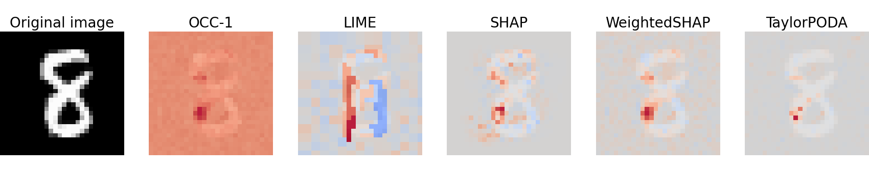
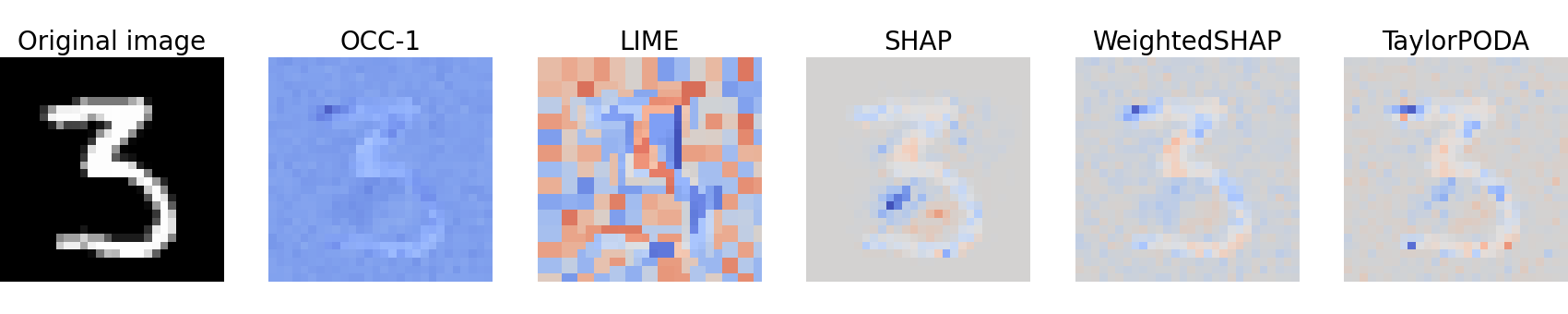
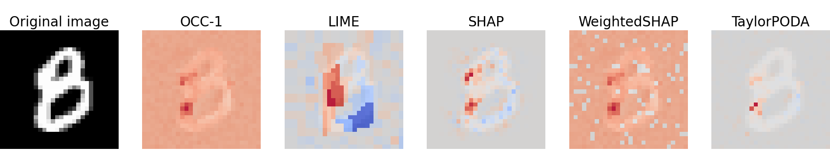
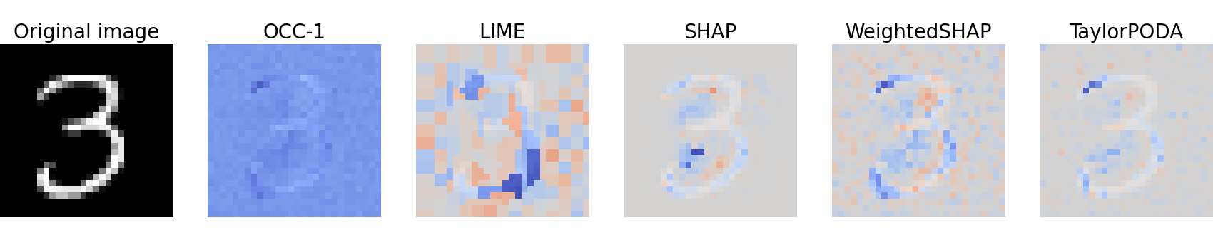
Figure 4: Illustrative examples of attributing model predictions for classifying digit-3 and digit-8 in MNIST. The pixels are color-coded: blue for negative, red for positive contribution to predicting “8”. TaylorPODA highlights the openness of the left segments of the upper and lower loops as the key discriminative regions. This observation appears to align with visual interpretation.

In particular, TaylorPODA consistently highlights the openness of the left segments of the upper and lower loops of digit “8” as key discriminative features—regions that effectively distinguish it from digit “3”.

5 Related work

Significant efforts have been made to enhance the explainability of opaque models. Early methods, such as partial dependence plots (Friedman, 2001) and individual conditional expectation (Goldstein et al., 2015), deeply incorporate visualizing the fluctuations in the model output by altering the feature values. Later, more specific post-hoc methods emerged. Ribeiro et al. (2016) proposed LIME, which builds an interpretable local surrogate for the original model. In parallel, LA methods were developed to attribute outputs to individual features. OCC-1 (Zeiler and Fergus, 2014), based on prediction difference (Robnik-Šikonja and Kononenko, 2008), computes LA by masking target features. Štrumbelj and Kononenko (2014) extended Shapley value (Shapley, 1953) to opaque models in AI context. Lundberg and Lee (2017) introduced SHAP and its popular implementation, which inspired many variants (Frye et al., 2020; Aas et al., 2021; Watson, 2022). Among them, WeightedSHAP (Kwon and Zou, 2022) relaxes SHAP’s “local accuracy” to adopt a more flexible semi-value (Dubey and Weber, 1977; Hart and Mas-Colell, 1989), and uses AUP to better align attributions with instance-level feature importance orderings.

Building on feature coalition-level attribution, Sundararajan et al. (2020) proposed the Shapley-Taylor Interaction Index, assigning scores to feature subsets and relating them to Taylor expansion terms. While this captures interactions, it introduces scalability and interpretability issues as subset numbers grow exponentially. To focus on individual feature-level attributions, Deng et al. (2024) proposed a Taylor expansion framework (see Section 2.1) that unifies various post-hoc methods, including Shapley-based ones.

6 Discussion

This paper leverages the Taylor expansion framework to identify two key sources of inaccuracy in LA—(F1) and (F2)—and proposes three postulates: precision, federation, and zero-discrepancy. Guided by these principles, we introduce TaylorPODA, which also incorporates an adaptation property for objective-aligned optimization based on instance-specific feature importance. Its effectiveness is supported by both theoretical analysis and empirical results. To the best of our knowledge, TaylorPODA is the first LA method fully grounded in the Taylor framework and the only one satisfying all the postulates and property. Nonetheless, improving the computational efficiency of TaylorPODA remains an open direction. As defined in (15), full evaluation requires computing $2^{|G|-1}$ Harsanyi dividends, each involving $2^{|S|}$ masked output queries. While experiments in Figure 4 show that truncating $|S|$ yields results consistent with human intuition, more advanced approximations are needed. Also, the development of more refined optimization strategies is warranted, for which we adopt Dirichlet-based random search in this work as a starting point.

Appendix A Proof of postulate and property satisfaction: TaylorPODA and other methods

Given a to-be-explained input-output pair $(\mathbf{x},f(\mathbf{x}))$, under a Taylor-expansion framework, a LA generates a group of contribution scores $\boldsymbol{a}=(a_{1},\dots,a_{d})$ with $a_{i}\in\mathbb{R}$ for $i\in G$, where the component $a_{i}$ measures the contribution of the corresponding $x_{i}$ by linearly combining the Taylor independent effects and the Taylor interaction effects within $f(\mathbf{x})$:

$$a_{i}(\mathbf{x},f(\mathbf{x}))=\sum_{j\in G}\sum_{\boldsymbol{\phi}\in\Pi_{\{j\}}}\tau_{i,j}\lambda(\boldsymbol{\phi})+\sum_{\begin{subarray}{c}S\subseteq G\\ |S|>1\end{subarray}}\sum_{\boldsymbol{\psi}\in\Pi_{S}}\zeta_{i,\psi}\mu(\boldsymbol{\psi}),$$ (20)

where $\tau_{i,j},\zeta_{i,\psi}\in\mathbb{R}$. The weight $\tau_{i,j}$ quantifies the proportion of the Taylor independent effect $\lambda(\boldsymbol{\phi})$ from the $j$-th feature attributed to $x_{i}$. Similarly, the weight $\zeta_{i,\psi}$ represents the proportion of the Taylor interaction effect $\mu(\boldsymbol{\psi})$ from the features in $S$ attributed to $x_{i}$.

TaylorPODA, as a LA, produces the attribution outcome for feature $i$ as follows. Let $\xi_{i,S}\in(0,1)$ for $S\subseteq G$ and $i\in S$, satisfying $\sum_{i\in S}\xi_{i,S}=1$:

$$\underset{(\text{TaylorPODA})}{a_{i}(\mathbf{x},f(\mathbf{x}))} =f(\mathbf{x})-f_{G\backslash{i}}(\mathbf{x})-\sum_{\begin{subarray}{c}S\subseteq G\\ |S|>1\\ i\in S\end{subarray}}(1-\xi_{i,S})H(S),$$ (21)

which is equivalent to

$$\underset{(\text{TaylorPODA})}{a_{i}(\mathbf{x},f(\mathbf{x}))}=\sum_{j=i}\sum_{\boldsymbol{\phi}\in\Pi_{\{j\}}}\lambda(\boldsymbol{\phi})+\sum_{\begin{subarray}{c}S\subseteq G\\ |S|>1\\ i\in S\end{subarray}}\sum_{\boldsymbol{\psi}\in\Pi_{S}}\xi_{i,S}\mu(\boldsymbol{\psi}).$$ (22)

Moreover, TaylorPODA meets Postulates 1, 2, 3, and Property 1, whereas other methods (OCC-1, LIME, SHAP, WeightedSHAP) fail to satisfy all of these postulates and the property collectively:

Postulate 1. Precision. The Taylor independent effect of the $i$-th feature shall be entirely attributed to the $i$-th feature, while it shall not be attributed to any other feature:

$$\tau_{i,j}=$$ (23)

Postulate 2. Federation. The Taylor interaction effect of the features in $S$ shall only be attributed to the features inside $S$:

$$\zeta_{i,\psi}=0,\quad\text{for all }i\notin S,\ \boldsymbol{\psi}\in\Pi_{S}.$$ (24)

Postulate 3. Zero-discrepancy. There should be neither redundancy nor deficiency in the attribution results regarding the allocation of the exact model output $f(\mathbf{x})$ to individual features. Equivalently, the value of discrepancy, denoted by $d(\mathbf{x},f;\boldsymbol{\beta};\mathbf{a})$ shall equal zero:

$$d(\mathbf{x},f;\boldsymbol{\beta};\mathbf{a})=f(\boldsymbol{\beta})+\sum_{i\in G}a_{i}(\mathbf{x},f(\mathbf{x}))-f(\mathbf{x})=0.$$ (25)

Property 1. Adaptation. For the $i$-th feature, the proportion of attribution from each Taylor interaction effect $\mu(\boldsymbol{\psi})$ with $\boldsymbol{\psi}\in\Pi_{S}$ and $S\subseteq G\setminus\{i\},|S|>1$ shall be tunable. Specifically, the attribution mechanism allows $\zeta_{i,\boldsymbol{\psi}}\in\left[0,1\right]$ for all $\boldsymbol{\psi}\in\Pi_{S}$ with $S\subseteq G,|S|>1,i\in S$.

Proof:

According to Theorem 2 in Deng et al. [2024], we have:

$$f(\mathbf{x})-f_{G\backslash\{i\}}(\mathbf{x})=\sum_{j=i}\sum_{\boldsymbol{\phi}\in\Pi_{\{j\}}}\lambda(\boldsymbol{\phi})+\sum_{\begin{subarray}{c}S\subseteq G\\ |S|>1\\ i\in S\end{subarray}}\sum_{\boldsymbol{\psi}\in\Pi_{S}}\mu(\boldsymbol{\psi}).$$ (26)

Also, according to Theorem 1 in Deng et al. [2024], we have

$$H(S)=\sum_{\boldsymbol{\psi}\in\Pi_{S}}\mu(\boldsymbol{\psi}),\forall S\in G,|S|>1.$$ (27)

Substituting (26) and (27) into (21), we get

$$\underset{(\text{TaylorPODA})}{a_{i}(\mathbf{x},f(\mathbf{x}))} =f(\mathbf{x})-f_{G\backslash\{i\}}(\mathbf{x})-\sum_{\begin{subarray}{c}S\subseteq G\\ |S|>1\\ i\in S\end{subarray}}(1-\xi_{i,S})H(S)$$ (28)

$$=\sum_{j=i}\sum_{\boldsymbol{\phi}\in\Pi_{\{j\}}}\lambda(\boldsymbol{\phi})+\sum_{\begin{subarray}{c}S\subseteq G\\ |S|>1\\ i\in S\end{subarray}}\sum_{\boldsymbol{\psi}\in\Pi_{S}}\mu(\boldsymbol{\psi})-\sum_{\begin{subarray}{c}S\subseteq G\\ |S|>1\\ i\in S\end{subarray}}(1-\xi_{i,S})H(S)$$

$$=\sum_{j=i}\sum_{\boldsymbol{\phi}\in\Pi_{\{j\}}}\lambda(\boldsymbol{\phi})+\sum_{\begin{subarray}{c}S\subseteq G\\ |S|>1\\ i\in S\end{subarray}}H(S)-\sum_{\begin{subarray}{c}S\subseteq G\\ |S|>1\\ i\in S\end{subarray}}(1-\xi_{i,S})H(S)$$

$$=\sum_{j=i}\sum_{\boldsymbol{\phi}\in\Pi_{\{j\}}}\lambda(\boldsymbol{\phi})+\sum_{\begin{subarray}{c}S\subseteq G\\ |S|>1\\ i\in S\end{subarray}}\sum_{\boldsymbol{\psi}\in\Pi_{S}}\xi_{i,S}\mu(\boldsymbol{\psi}).$$

Thus, TaylorPODA defined in (21) is equivalent to (22). Moreover, by setting $\tau_{i,j}=1$ and $\zeta_{i,\psi}=\xi_{i,S}$ for $\psi\in\Pi_{S}$, (20) can be equivalently written as (22).

Therefore, when calculating $\underset{(\text{TaylorPODA})}{a_{i}(\mathbf{x},f(\mathbf{x}))}$ only the Taylor independent effect of the $i$-th feature, i.e., $\sum_{j=i}\sum_{\boldsymbol{\phi}\in\Pi_{\{j\}}}\lambda(\boldsymbol{\phi})$, are involved without any other features $j\neq i$, as demonstrated by (21). Thus, TaylorPODA satisfies Postulate 1. Similarly, according to (8) and (7), OCC-1 and SHAP satisfy Postulate 1. As demonstrated in (9), WeightedSHAP attributes Taylor independent effects with a weighting factor $w_{S}$, thereby violating Postulate 1.

As indicated in (22), the Taylor interaction effects will be attributed to the $i$-th feature, if and only if $S\subseteq G\$ with $\ i\in S$ and $|S|>1$. Thus, TaylorPODA satisfies Postulate 2. Similarly, according to (8), (7), and (9), it can be found that OCC-1, SHAP, and WeightedSHAP satisfy Postulate 1.

As for discrepancy, we have

$$f(\boldsymbol{\beta})+\sum_{i\in G}\underset{(\text{TaylorPODA})}{a_{i}(\mathbf{x},f(\mathbf{x}))}$$ (29)

$$= f(\boldsymbol{\beta})+\sum_{i\in G}\left[\sum_{j=i}\sum_{\boldsymbol{\phi}\in\Pi_{\{j\}}}\lambda(\boldsymbol{\phi})+\sum_{\begin{subarray}{c}S\subseteq G\\ |S|>1\\ i\in S\end{subarray}}\xi_{i,S}\sum_{\boldsymbol{\psi}\in\Pi_{S}}\mu(\boldsymbol{\psi})\right]$$

$$= f(\boldsymbol{\beta})+\sum_{i\in G}\sum_{\boldsymbol{\phi}\in\Pi_{\{i\}}}\lambda(\boldsymbol{\phi})+\sum_{i\in G}\sum_{\begin{subarray}{c}S\subseteq G\\ |S|>1\\ i\in S\end{subarray}}\xi_{i,S}\sum_{\boldsymbol{\psi}\in\Pi_{S}}\mu(\boldsymbol{\psi}).$$

Given that $\sum_{i\in S}\xi_{i,S}=1$ for $S\subseteq G$, (29) can be further transformed into:

$$f(\boldsymbol{\beta})+\sum_{i\in G}\underset{(\text{TaylorPODA})}{a_{i}(\mathbf{x},f(\mathbf{x}))}=f(\boldsymbol{\beta})+\sum_{\begin{subarray}{c}S\subseteq G\\ |S|>1\end{subarray}}\sum_{\boldsymbol{\phi}\in\Pi_{\{i\}}}\lambda(\boldsymbol{\phi})+\sum_{i\in G}\sum_{\boldsymbol{\psi}\in\Pi_{S}}\mu(\boldsymbol{\psi})=f(\mathbf{x}).$$ (30)

Thus, TaylorPODA satisfies Postulate 3. Similarly, as given in (8), we can equivalently have $\zeta_{i,S}=1$ for $i\in G$ and $S\subseteq G$ with $|S|>1$, so that $\sum_{\begin{subarray}{c}S\subseteq G\\ |S|>1\\ i\in S\end{subarray}}\xi_{i,S}>1$ for OCC-1. Similarly again, as given in (7), we can equivalently have $\xi_{i,S}=1/|S|$ for $i\in G$ and $S\subseteq G$ with $|S|>1$, so that $\sum_{\begin{subarray}{c}S\subseteq G\\ |S|>1\\ i\in S\end{subarray}}\xi_{i,S}=1$ for SHAP. However, as the weighting factor $\omega_{S}$ is not limited in terms of its sum value, it is not ensured that $\sum_{\begin{subarray}{c}S\subseteq G\\ |S|>1\\ i\in S\end{subarray}}\xi_{i,S}=1$ in WeightedSHAP. Thus, SHAP satisfies Postulate 3, whereas OCC-1 and WeightedSHAP violate Postulate 3.

Moreover, as $\xi_{i,S}$ is an adaptive weight, essentially, the exact quantity of the Taylor interaction that is to be allocated to the $i$-th feature is adjustable, instead of setting a fixed ratio. Thus, TaylorPODA introduces (satisfies) Property 1. Similarly, according to (8), (7), and (9), it can be found that WeightedSHAP satisfies Property 1, whereas OCC-1 and SHAP violate Property 1.

As for LIME, it should not be regarded as a strict LA method or even an attributional method for allocating the contribution of each feature in $f(\mathbf{x})$, since it explains models by introducing an external surrogate model $g(\mathbf{x})$ to approximate the original model, as shown by (10) and (11). Consequently, LIME falls outside the scope of the postulate (property) system in this work, and its corresponding columns in Table 2 are marked with “–”.

This completes the proof. $\blacksquare$

Appendix B Implementation Details of the Experiments

All experiments were conducted on a machine equipped with a 13th Gen Intel^® Core™ i7-13700K CPU (3.40 GHz) and 32 GB RAM.

The datasets and the corresponding prediction tasks:

Seven tabular datasets together with a two-dimensional image dataset are used for the experiments in Section 4, all of which are publicly available. Based on these datasets, the corresponding prediction tasks are designed. Details of these datasets and the are shown as follows:

Table 4: Details of the datasets and the corresponding prediction tasks used for the experiments in Section 4.

Dataset	Size	Features	Task	Source
Cancer	683	Clump_thickness, Uniformity_of_cell_size, Uniformity_of_cell_shape, Marginal_adhesion, Single_epithelial_cell_size, Bare_nuclei, Bland_chromatin, Normal_nucleoli, Mitoses	Classifying whether the (Class) of the cancer is benign or malignant.	https://archive.ics.uci.edu/dataset/15/breast+cancer+wisconsin+original
Rice	3810	Area, Perimeter, Major_Axis_Length, Eccentricity, Convex_Area, Extent	Classifying whether the rice specie (Class) is Osmancik or Cammeo.	https://archive.ics.uci.edu/dataset/545/rice+cammeo+and+osmancik
Titanic	712	Age, Fair, Pclass, Sibsp, Parch, Alone, Adult_male	Classifying whether the passenger is survival or not.	https://www.kaggle.com/c/titanic/data
Abalone	4177	Sex, Length, Height, Whole_weight, Shucked_weight, Viscera_weight, Shell_weight	Predicting the age (rings) of abalone from physical measurements.	https://archive.ics.uci.edu/dataset/1/abalone
California	20640	MedInc, HouseAge, AveRooms, AveBedrms, Population, AveOccup, Latitude, Longitude	Predicting the median house value (MedHouseVal) of California districts from demographic and geographic information.	https://scikit-learn.org/1.5/modules/generated/sklearn.datasets.fetch_california_housing.html
Concrete	1030	Cement, Blast furnace slag, Fly ash, Water, Superplasticizer, Coarse aggregate, Fine aggregate, Age	Predicting the compressive strength of concrete mixtures from their ingredients and age.	https://archive.ics.uci.edu/dataset/165/concrete+compressive+strength
MNIST38∗	13966	Two-dimensional grayscale image pixels	Classifying the digits 3 and 8 from the hand-written numbers.	https://keras.io/api/datasets/mnist/

All datasets are shuffled, with 80% of the samples in each set randomly selected for training. Attribution experiments are conducted using 100 hold-out samples randomly drawn from the remaining 20%.

^∗The $28\times 28$ MNIST38 dataset is obtained from the original MNIST dataset by extracting all the digit-3 and digit-8 images while excluding the images of other digits.

The task models:

For the prediction tasks with all the datasets, we adopt machine learning-based fully connected multi-layer perceptron (MLP).

Regarding differentiability, it is important to note that all activation functions used in the quantitative analysis presented in the main body (specifically, the experiments related to Table 3)—namely, tanh and logistic—are continuously differentiable. As a result, the MLP-based task models are fully differentiable, enabling proper evaluation and analysis within the Taylor framework.

Furthermore, the additional experimental results on non-differentiable models (and the details of the models) are shown in Appendix D.

For the classification tasks in this study, we explain the model predictions based on the predicted probability of the positive class (label=1) rather than the final classification result (e.g., top-1 label). That is, the analysis is conducted with respect to the model’s continuous output — the estimated probability — rather than its discrete decision outcome.

Setup for fair comparison of TaylorPODA and the other baseline LA methods:

As discussed in Section 2 and 3, our proposed TaylorPODA, together with the existing OCC-1, SHAP, and WeightedSHAP, can be generalized as LA methods, thereby sharing similar calculation process. To establish fair comparison of TaylorPODA and the other LA baselines in the experiments, we further set up the corresponding parameters and designs by making full use of the similarity.

• Since these LA methods rely on the masked outputs of the task models, they are configured to utilize a shared masked output calculator by incorporating one of the sub-functions weightedSHAP.generate_coalition_function provided within the WeightedSHAP package (https://github.com/ykwon0407/WeightedSHAP, used with the author’s permission).

• According to Kwon and Zou [2022] and the default settings of the WeightedSHAP package, WeightedSHAP generates solution candidates based on 16 distinct weight distributions. To ensure a relatively fair comparison, we similarly configure the search process of this version of TaylorPODA to include 16 distinct solution candidates. These candidates are generated from the Dirichlet distribution ($\alpha_{i}=1$ for all $i\in G$), as discussed in Section 3.3.

• For the quantitative experimental results presented in Table 3, 5, and 6, we reimplemented a full version of SHAP without the subset sampling approximation, in accordance with (7), to avoid certain automatic approximation heuristics in the standard SHAP implementation. Similarly, we reimplemented a complete version of OCC-1 based on (8). This was done to faithfully follow the theoretical formulations and ensure consistency with the sharing use of the same masked outputs.

• For the qualitative experimental results presented in Figure 4, we adopted SHAP (version 0.44.0, MIT license)’s PermutationExplainer to accommodate the use of approximation techniques. For LIME (version 0.2.0.1, BSD-2-Clause license), we utilized the LimeImageExplainer tailored for image data.

Appendix C Heuristic approximation of TaylorPODA

Although TaylorPODA offers a theoretically principled attribution method based on the full Taylor expansion, its direct application to high-dimensional data becomes infeasible due to the combinatorial explosion of high-cardinality interaction terms. As an initial step toward improving scalability and showcasing the potential of TaylorPODA on high-dimensional datasets, we propose a heuristic approximation (TaylorPODA-c$\sigma$) that preserves only low-cardinality terms over a restricted subset of input features:

$$\underset{(\text{TaylorPODA})}{a_{i}(\mathbf{x},f(\mathbf{x}))}\approx\underset{(\text{TaylorPODA-c})}{a_{i}^{(\sigma)}(\mathbf{x},f(\mathbf{x}))}=f(\mathbf{x})-f_{G\backslash\{i\}}(\mathbf{x})-\sum_{\begin{subarray}{c}S\subseteq G\\ 1<|S|\leq\sigma\\ i\in S\end{subarray}}(1-\xi_{i,S})H(S),$$ (31)

where $\sigma\in G$ with $\sigma>1$ denotes an upper bound on the cardinality of $S$. Accordingly, as $\sigma=1,2,\dots,|G|,\quad a_{i}^{(\sigma)}(\mathbf{x},f(\mathbf{x}))\to a_{i}(\mathbf{x},f(\mathbf{x}))$ With a determined bound $\sigma$, the value gap $\Delta$ between the attribution results produced by TaylorPODA-c and the full TaylorPODA is:

$$\Delta(\sigma) =\underset{(\text{TaylorPODA-c})}{a_{i}^{(\sigma)}(\mathbf{x},f(\mathbf{x}))}-\underset{(\text{TaylorPODA})}{a_{i}(\mathbf{x},f(\mathbf{x}))}$$ (32)

$$=\sum_{\begin{subarray}{c}S\subseteq G\\ |S|>1\\ i\in S\end{subarray}}(1-\xi_{i,S})H(S)-\sum_{\begin{subarray}{c}S\subseteq G\\ 1<|S|\leq\sigma\\ i\in S\end{subarray}}(1-\xi_{i,S})H(S)$$

$$=\sum_{\begin{subarray}{c}S\subseteq G\\ |S|>\sigma\\ i\in S\end{subarray}}(1-\xi_{i,S})H(S).$$

And we have $\Delta(\sigma)=0$ when $\sigma=|G|$.

By upper-bounding the cardinality of the features, this approximation approach aligns with the insight of [Ren et al., 2024], which suggests that “under these conditions, the DNN will only encode a relatively small number of sparse interactions between input variables.” While more sophisticated and broadly applicable approximation methods—extending beyond differentiable DNNs and the specific conditions considered in [Ren et al., 2024]—remain an open direction for future work, we believe this heuristic provides a reasonable and principled starting point.

Appendix D Additional experimental results on non-differentiable models

MLP with ReLU:

Table 5: Importance ordering performance on 100 hold-out test samples with MLP models and ReLU activation.

	Classification			Regression
Method	Data	AUP	Inclusion AUC	Data	AUP	Inclusion MSE ($\times 10^{-2}$)
OCC-1	Cancer	1.0424 (0.8177, 1.2671)	0.8933 (0.8553, 0.9314)	Abalone	0.1424 (0.1239, 0.1609)	0.0674 (0.0472, 0.0875)
LIME		0.2880 (0.1989, 0.3770)	0.9889 (0.9742, 1.0000)		0.1452 (0.1279, 0.1626)	0.0569 (0.0421, 0.0718)
SHAP		0.2411 (0.1392, 0.3431)	0.9833 (0.9666, 1.0000)		0.1709 (0.1525, 0.1894)	0.0684 (0.0525, 0.0843)
WeightedSHAP		0.1609 (0.1096, 0.2121)	0.9911 (0.9810, 1.0000)		0.1032 (0.0913, 0.1152)	0.0343 (0.0266, 0.0421)
TaylorPODA		0.1700 (0.1057, 0.2342)	0.9911 (0.9774, 1.0000)		0.0982 (0.0854, 0.1110)	0.0300 (0.0222, 0.0378)
OCC-1	Rice	0.4569 (0.3593, 0.5545)	0.9514 (0.9262, 0.9767)	California	0.1767 (0.1517, 0.2016)	0.1367 (0.1007, 0.1726)
LIME		0.1110 (0.0762, 0.1458)	0.9971 (0.9932, 1.0000)		0.2694 (0.2382, 0.3006)	0.3036 (0.2303, 0.3769)
SHAP		0.1176 (0.0795, 0.1557)	0.9857 (0.9734, 0.9980)		0.1900 (0.1653, 0.2147)	0.1417 (0.1047, 0.1788)
WeightedSHAP		0.0930 (0.0621, 0.1240)	0.9914 (0.9810, 1.0000)		0.1410 (0.1207, 0.1614)	0.0973 (0.0692, 0.1254)
TaylorPODA		0.0679 (0.0475, 0.0882)	0.9971 (0.9932, 1.0000)		0.1583 (0.1348, 0.1818)	0.1108 (0.0782, 0.1434)
OCC-1	Titanic	0.3298 (0.2926, 0.3671)	0.9957 (0.9895, 1.0000)	Concrete	0.3619 (0.3117, 0.4122)	0.5512 (0.3558, 0.7466)
LIME		0.6296 (0.5349, 0.7243)	0.9443 (0.9120, 0.9766)		0.3555 (0.3234, 0.3877)	0.3880 (0.3200, 0.4560)
SHAP		0.4832 (0.4364, 0.5300)	0.9771 (0.9544, 0.9999)		0.2730 (0.2474, 0.2985)	0.2598 (0.2150, 0.3046)
WeightedSHAP		0.3218 (0.2852, 0.3585)	0.9971 (0.9915, 1.0000)		0.2225 (0.2009, 0.2441)	0.1986 (0.1591, 0.2381)
TaylorPODA		0.4044 (0.3672, 0.4415)	0.9886 (0.9744, 1.0000)		0.2257 (0.2028, 0.2485)	0.2041 (0.1643, 0.2438)

Figure 5: Discrepancy performance on 100 hold-out test samples with MLP models and ReLU activation.

XGboost:

Table 6: Importance ordering performance on XGBoost [Chen and Guestrin, 2016] models.

	Classification			Regression
Method	Data	AUP	Inclusion AUC	Data	AUP	Inclusion MSE ($\times 10^{-2}$)
OCC-1	Cancer	0.5996 (0.4375, 0.7618)	0.9478 (0.9222, 0.9734)	Abalone	0.2092 (0.1823, 0.2361)	0.1174 (0.0877, 0.1470)
LIME		0.3824 (0.3008, 0.4640)	0.9922 (0.9839, 1.0000)		0.2349 (0.2074, 0.2625)	0.1306 (0.0965, 0.1648)
SHAP		0.2795 (0.2188, 0.3402)	0.9978 (0.9947, 1.0000)		0.2257 (0.2031, 0.2482)	0.1072 (0.0843, 0.1301)
WeightedSHAP		0.2199 (0.1887, 0.2511)	1.0000 (1.0000, 1.0000)		0.1535 (0.1314, 0.1756)	0.0664 (0.0446, 0.0883)
TaylorPODA		0.2522 (0.2088, 0.2955)	1.0000 (1.0000, 1.0000)		0.1538 (0.1314, 0.1761)	0.0645 (0.0418, 0.0872)
OCC-1	Rice	0.5283 (0.4246, 0.6320)	0.9514 (0.9241, 0.9788)	California	0.2797 (0.2336, 0.3257)	0.2894 (0.1979, 0.3809)
LIME		0.3890 (0.2645, 0.5135)	0.9714 (0.9441, 0.9987)		0.4115 (0.3533, 0.4698)	0.5468 (0.3944, 0.6992)
SHAP		0.3246 (0.2115, 0.4376)	0.9729 (0.9463, 0.9995)		0.3623 (0.3091, 0.4154)	0.4207 (0.2931, 0.5482)
WeightedSHAP		0.2189 (0.1561, 0.2818)	0.9757 (0.9522, 0.9993)		0.2455 (0.2017, 0.2892)	0.2398 (0.1538, 0.3259)
TaylorPODA		0.2491 (0.1692, 0.3291)	0.9829 (0.9625, 1.0000)		0.3097 (0.2572, 0.3622)	0.3467 (0.2298, 0.4636)
OCC-1	Titanic	0.5835 (0.4955, 0.6714)	0.9529 (0.9168, 0.9889)	Concrete	0.5470 (0.4753, 0.6186)	0.9618 (0.7190, 1.2047)
LIME		1.1315 (0.9515, 1.0000)	0.8771 (0.8282, 0.9261)		0.6959 (0.6166, 0.7752)	1.3279 (1.0716, 1.5842)
SHAP		0.9155 (0.7826, 1.0000)	0.9329 (0.8963, 0.9694)		0.5737 (0.5087, 0.6386)	0.9035 (0.7236, 1.0834)
WeightedSHAP		0.5411 (0.4593, 0.6229)	0.9571 (0.9233, 0.9910)		0.4219 (0.3608, 0.4830)	0.6023 (0.4480, 0.7567)
TaylorPODA		0.7553 (0.6540, 0.8565)	0.9500 (0.9159, 0.9841)		0.4772 (0.4111, 0.5432)	0.7319 (0.5586, 0.9051)

Figure 6: Discrepancy performance on 100 hold-out test samples with XGBoost models.

References

- Aas et al. [2021] K. Aas, M. Jullum, and A. Løland. Explaining individual predictions when features are dependent: More accurate approximations to shapley values. Artificial Intelligence, 298:103502, 2021.
- Chen and Guestrin [2016] T. Chen and C. Guestrin. Xgboost: A scalable tree boosting system. In Proceedings of the 22nd acm sigkdd international conference on knowledge discovery and data mining, pages 785–794, 2016.
- Deng et al. [2024] H. Deng, N. Zou, M. Du, W. Chen, G. Feng, Z. Yang, Z. Li, and Q. Zhang. Unifying fourteen post-hoc attribution methods with taylor interactions. IEEE Transactions on Pattern Analysis and Machine Intelligence, 2024.
- Dubey and Weber [1977] P. Dubey and R. J. Weber. Probabilistic values for games. Cowles Foundation Discussion Papers, 1977.
- Friedman [2001] J. H. Friedman. Greedy function approximation: a gradient boosting machine. Annals of statistics, pages 1189–1232, 2001.
- Frye et al. [2020] C. Frye, C. Rowat, and I. Feige. Asymmetric shapley values: incorporating causal knowledge into model-agnostic explainability. Advances in neural information processing systems, 33:1229–1239, 2020.
- Goldstein et al. [2015] A. Goldstein, A. Kapelner, J. Bleich, and E. Pitkin. Peeking inside the black box: Visualizing statistical learning with plots of individual conditional expectation. journal of Computational and Graphical Statistics, 24(1):44–65, 2015.
- Harsanyi [1982] J. C. Harsanyi. A simplified bargaining model for the n-person cooperative game. Papers in game theory, pages 44–70, 1982.
- Hart and Mas-Colell [1989] S. Hart and A. Mas-Colell. Potential, value, and consistency. Econometrica: Journal of the Econometric Society, pages 589–614, 1989.
- Jethani et al. [2021] N. Jethani, M. Sudarshan, I. C. Covert, S.-I. Lee, and R. Ranganath. Fastshap: Real-time shapley value estimation. In International conference on learning representations, 2021.
- Kwon and Zou [2022] Y. Kwon and J. Y. Zou. Weightedshap: Analyzing and improving shapley based feature attributions. Advances in Neural Information Processing Systems, 35:34363–34376, Dec. 2022.
- LeCun et al. [1998] Y. LeCun, L. Bottou, Y. Bengio, and P. Haffner. Gradient-based learning applied to document recognition. Proceedings of the IEEE, 86(11):2278–2324, 1998.
- Lundberg and Lee [2017] S. M. Lundberg and S.-I. Lee. A unified approach to interpreting model predictions. Advances in neural information processing systems, 30, 2017.
- Ng et al. [2011] K. W. Ng, G.-L. Tian, and M.-L. Tang. Dirichlet and related distributions: Theory, methods and applications. John Wiley & Sons, 2011.
- Ren et al. [2024] Q. Ren, J. Gao, W. Shen, and Q. Zhang. Where we have arrived in proving the emergence of sparse interaction primitives in DNNs. In The Twelfth International Conference on Learning Representations, 2024.
- Ribeiro et al. [2016] M. T. Ribeiro, S. Singh, and C. Guestrin. “why should I trust you?”: Explaining the predictions of any classifier. In Proceedings of the 22nd ACM SIGKDD International Conference on Knowledge Discovery and Data Mining, San Francisco, CA, USA, August 13-17, 2016, pages 1135–1144, 2016.
- Robnik-Šikonja and Kononenko [2008] M. Robnik-Šikonja and I. Kononenko. Explaining classifications for individual instances. IEEE Transactions on Knowledge and Data Engineering, 20(5):589–600, 2008.
- Shapley [1953] L. S. Shapley. A value for n-person games. Contribution to the Theory of Games, 2, 1953.
- Štrumbelj and Kononenko [2014] E. Štrumbelj and I. Kononenko. Explaining prediction models and individual predictions with feature contributions. Knowledge and information systems, 41:647–665, 2014.
- Sundararajan et al. [2020] M. Sundararajan, K. Dhamdhere, and A. Agarwal. The shapley taylor interaction index. In International conference on machine learning, pages 9259–9268. PMLR, 2020.
- Watson [2022] D. Watson. Rational shapley values. In Proceedings of the 2022 ACM Conference on Fairness, Accountability, and Transparency, pages 1083–1094, 2022.
- Yeh [1998] I.-C. Yeh. Concrete Compressive Strength. UCI Machine Learning Repository, 1998. DOI: https://doi.org/10.24432/C5PK67.
- Zeiler and Fergus [2014] M. D. Zeiler and R. Fergus. Visualizing and understanding convolutional networks. In Computer Vision–ECCV 2014: 13th European Conference, Zurich, Switzerland, September 6-12, 2014, Proceedings, Part I 13, pages 818–833. Springer, 2014.