First-of-its-kind AI model for bioacoustic detection using a lightweight associative memory Hopfield neural network

Abstract

A growing issue within conservation bioacoustics is the task of analysing the vast amount of data generated from the use of passive acoustic monitoring devices. In this paper, we present an alternative AI model which has the potential to help alleviate this problem. Our model formulation addresses the key issues encountered when using current AI models for bioacoustic analysis, namely the: limited training data available; environmental impact, particularly in energy consumption and carbon footprint of training and implementing these models; and associated hardware requirements. The model developed in this work uses associative memory via a transparent, explainable Hopfield neural network to store signals and detect similar signals which can then be used to classify species. Training is rapid ($3$ ms), as only one representative signal is required for each target sound within a dataset. The model is fast, taking only $5.4$ s to pre-process and classify all $10384$ publicly available bat recordings, on a standard Apple MacBook Air. The model is also lightweight with a small memory footprint of $144.09$ MB of RAM usage. Hence, the low computational demands make the model ideal for use on a variety of standard personal devices with potential for deployment in the field via edge-processing devices. It is also competitively accurate, with up to $86\%$ precision on the dataset used to evaluate the model. In fact, we could not find a single case of disagreement between model and manual identification via expert field guides. Although a dataset of bat echolocation calls was chosen to demo this first-of-its-kind AI model, trained on only two representative calls, the model is not species specific. In conclusion, we propose an equitable AI model that has the potential to be a game changer for fast, lightweight, sustainable, transparent, explainable and accurate bioacoustic analysis.

[wolves]organization=Department of Computing and Mathematical Sciences, University of Wolverhampton,addressline=Wulfruna Street, city=Wolverhampton, postcode=WV1 1LY, country=UK

1 Introduction

The combination of passive acoustic monitoring (PAM), via the use of autonomous recording units (ARUs), and bioacoustic analysis is a cost-effective, non-invasive and sustainable method increasingly used for ecological discovery, monitoring and conservation in most known ecosystems around the globe (Abrahams and Geary, 2020; Bakker, 2022; Bradfer-Lawrence et al., 2023; Teixeira et al., 2019). Even when PAM is implemented with the use of careful and consistent guidelines and methods (Metcalf et al., 2023; Pérez-Granados and Traba, 2021) it still has obvious limitations and does not replace experts working in the field. With the increase in lower cost ARUs, such as the Apodemus Pippyg, Audiomoth, Song Meter and even custom made devices (Apodemus Field Equipment, 2025; Hill et al., 2019; Mydlarz et al., 2017; Wildlife Acoustics, 2024) and the potential of biodegradable sensors (Sethi et al., 2022), ecologists and conservationists are now able to leverage new digital and computational technologies for PAM. Given the consequences of rampant biodiversity loss on a warming planet, the vast amount of data collected daily and the limitations of commercial classifiers currently available, there exists an urgent need for new efficient automated analysis tools and software to alleviate the processing bottleneck (Goodwin and Gillam, 2021; Kershenbaum et al., 2025; Mac Aodha et al., 2018; McEwen et al., 2024; Stowell, 2022) without compromising ecological and conservation goals and values (Sandbrook, 2025).

Automated techniques to analyse PAM datasets initially involved machine learning via statistical models and ensemble learning and are still used successfully. For example, researchers have used random forest models (Yoh et al., 2022) and many researchers and fieldworkers use Kaleidoscope Pro where, in auto-ID mode, a species-level Hidden Markov Model is created and the results are obtained via clustering analysis (Wildlife Acoustics, 2017; Manzano-Rubio et al., 2022). However, deep learning and specifically convolutional neural networks (CNNs) currently dominate academic research on automated bioacoustic classification (Kershenbaum et al., 2025; Rasmussen et al., 2024; Stowell, 2022). CNNs are commonly used for image classification and hence require bioacoustic data to be converted to spectrograms with set dimensions dependent upon the particular architecture of the model, a process which is costly in terms of time, memory and energy. CNNs are considered to be ‘black boxes’ that lack transparency, are computationally expensive and challenging to explain. In ecology and conservation, pretrained models, such as BirdNet (Kahl et al., 2021), are popular with architecture most frequently based on the ResNet family of CNN models (Kahl et al., 2021; MacIsaac et al., 2024; Salem et al., 2024; Dufourq et al., 2022). Although such models show potential and consistent improvement they have yet to be fully proven (Funosas et al., 2024; Pérez-Granados, 2023). CNNs are rapidly being superseded by transformer architecture Dosovitskiy et al. (2020), the architecture driving large language models such as ChatGPT, where GPT is the acronym for generative pre-trained transformer. These vision transformer (ViT) models are now slowly being adopted by the bioacoustic research community (McEwen et al., 2024; Ferreira et al., 2025). Additionally, and inspired by ViT architecture, a new generation of CNNs, ConvNeXts, has emerged and is producing promising results (Liu et al., 2022). Heinrich et al. (2025) combine a ConvNeXt with a ProtoPNet, a prototypical part network (Chen et al., 2019) to produce a more interpretable model for bird sound classification.

All deep learning methods, with their multilayer architecture, are computationally expensive (Thompson et al., 2021). They require extensive preprocessing of data, up-to-date hardware (CPUs, GPUs and large amounts of RAM) and are usually performed on high performance computing clusters often at Global North institutes (Kahl et al., 2021; MacIsaac et al., 2024). Not all researchers and few fieldworkers have access to these high performance facilities and expensive hardware. For instance, the single GPU used in Heinrich et al. (2025), an NVIDIA A100-SXM4-80GB GPU, currently costs £13,800 for the graphics card alone. Training times tend not to be documented in the bioacoustics research literature, although they can be anything from 16 minutes to 2.5 hours per epoch; in Heinrich et al. (2025) each model is trained for 10 epochs. Furthermore, the environmental impact of the pre-trained models themselves should not be dismissed (Thompson et al., 2021; Toews, R., 2020), as with all industries, use justifies retraining, which in turn uses massive amounts of energy. For example, training the ResNet-50 on a NVIDIA M40 GPU takes 14 days (You et al., 2018). For those researchers looking to estimate their training carbon footprint when using deep learning models, Bouza et al. (2023) provide an introduction to energy consumption tracking tools.

Deep learning models require extremely large datasets for pretraining such as ImageNet; however, we cannot assume that the labelling of such datasets is accurate nor that higher capacity CNN models, such as the later ResNet models, will demonstrate better real-world performance than low capacity models as detailed in Northcutt et al. (2021). Therefore, layers which have been pretrained will still maintain any legacy/bias learning from the pretrained model. Additionally, the bioacoustic WAV datasets used to train the final layers are mainly examples of weakly labelled data (Planque, B., 2024), where an entire recording has a single label which is segmented for training. Each segment will then have the same label despite other species or absences being present within the same recording (Planque, B., 2024). Activity detectors are used to partly alleviate this problem (Ghani et al., 2023). A third data issue with all these deep learning methods is that they require balanced datasets which are often unavailable, especially for rare species or specific calls. Data augmentation is having some success (MacIsaac et al., 2024) and pretrained transformer models perform well even on smaller training sets (McEwen et al., 2024; Ferreira et al., 2025), but all still require significant amounts of labelled data and the use of high performance computing centres for pretraining and transfer learning. These intensive demands mean that some researchers resort to, and in some cases prefer, manual analysis of sound files and spectrograms, to ensure rare events are discovered and any classification is accurate (Szesciorka et al., 2023), while Sandbrook (2025) warns practitioners of the unintended consequences of the use of AI for conservation.

For researchers looking to make event detections amongst the large numbers of PAM generated files, automated approaches are absolutely invaluable if they are efficient, transparent and sustainable enough to justify their use; ideally, incorporated into edge-processing devices or in active learning approaches of human-computer interaction (Stowell, 2022). The digital age has enabled us to enhance many of our own capacities. In this work, we enhance and augment the listening and recognition capabilities of ecologists and conservationists and the recorders they use in the field today with a new approach of using a neural assosiative memory network that can be trained and deployed on a standard working laptop and used to detect specific bioacoustic events. The human ear and brain constitute a listening, sound storage and recall device which has definite limitations, namely, processing capacity and speed, and the frequency range within which detections can be made, $20$ Hz to $20$ kHz for the human auditory range (Brownell, 1997; Dobie and Van Hemel, 2004). Digital listening devices and AI can listen to and process at speed a broader range of sounds with varying power thresholds and filters, and as such can significantly augment our own abilities. Biologically inspired neural associative memory networks, such as those first conceptualised in Hopfield (1982) and used here, simulate the associative memory process by storing patterns which may then be recalled/retrieved from noisy or partial patterns, and are thus examples of content-addressable memory systems. John Hopfield’s contribution to AI was acknowledged when he jointly won the Nobel Prize in Physics in October 2024 (NobelPrize.org, 2024). Hopfield neural networks (HNNs) have been developed and implemented on a number of tasks such as image recognition and optimisation (Dai and Nakano, 1998; Liu et al., 2023) with further improvements made by incorporating characteristics of chaotic dynamics to overcome the tendency of HNNs to converge to non-optimal solutions (Chen and Aihara, 1995; Rodden et al., 2024). In this work, we couple an HNN with augmented ‘hearing’ and demonstrate how this type of neural network can address some of the challenges facing the field of bioacoustics. The model in this paper can be developed without the need for large training datasets, ’black box’ multilayer networks and expensive resource-intensive hardware and training times. We use an inherently interpretable associative memory neural network model which does not use any image processing techniques. As this model has not been used for bioacoustic event detection before, we use a public bioacoustic dataset developed to facilitate the research of automated classification techniques (Bertran Ferrer, 2019; Bertran et al., 2019). As befits the introduction and explanation of a new model to the field, the classification task chosen is relatively simple: to identify the echolocation pulses of two cryptic bat species. Our model is fast, taking only $5.4$ seconds to train, pre-process and classify all $10384$ publicly available bat recordings (Bertran Ferrer, 2019; Bertran et al., 2019), on a standard Apple MacBook Air. The model is also lightweight, i.e., it has a small memory footprint of $144.09$ MB of RAM usage. These low computational demands make the model ideal for use on a variety of standard personal devices with potential for deployment in the field via edge-processing devices.

This paper is organised as follows. Firstly, in section 2 we outline the dataset used to evaluate our model including its source, structure and relevance for AI model development. In section 3 we outline how the model is developed from the underlying theory of Hopfield networks and how patterns are stored in its memory, to the augmentation of hearing onto the model via the fast Fourier transform. In section 4 we present the results and performance metrics of the model and discuss these results in section 5 highlighting the key issues and consequences for this model application.

2 Material and methods

Here we principally explain the dataset used for model development and testing. Bats were chosen as the sound source for this study. Bats are protected in Europe and the UK, and considered to be indicators of biodiversity (Catto et al., 2003). All UK species are nocturnal and therefore bat surveyors are partially dependent upon acoustic data to survey and monitor their populations. Furthermore, there is a long tradition of studying bat echolocation pulses since the pioneering work of Griffin and Pierce in the 1930s (Pierce and Griffin, 1938). Additionally, because the majority of bat vocalisations and echolocation calls are in the ultrasonic frequency range - that is above the frequency at which humans can hear - fieldworkers use a combination of heterodyne (where signals are shifted into the audible frequency range), time-expansion techniques (where the sound is slowed down to the audible range), and spectrograms (visual representations of the signals) to manually identify species. Unsurprisingly, these manual techniques run into problems in large surveys with many thousands of hours of data to slow down and analyse.

The split dataset used in this work was created by Bertran et al. (2019), the authors of this paper had two problems in mind:

• Identifying two cryptic, or morphologically similar, bat species - Pipistrellus pipistrellus, or the Common pipstrelle (PIPI), and Pipstrellus pygmaeus or Soprano pipistrelle (PIPY) - species which were not considered to be distinct until the late 1990s (Barlow and Jones, 1999).

• Creating a dataset suited to training AI models in order to identify these two species in urban environments where man-made sources of ultrasonic sounds are also present.

The signals were recorded by Elena Tena, a co-author of Bertran et al. (2019), in an Iberian forest in the Guadarrama Mountains between 2016 and 2018; an area with very little man-made sonic pollution. Echo Meter Touch Pro 1 bat detectors were used to capture the echolocation sequences and filtered using Kaleidoscope (Wildlife Acoustics, Inc., USA). Analysis and labelling were completed via commercial software, BatSound 4 (Pettersson Elektronik AB, Upsala Sweden), and expert manual confirmation (Bertran et al., 2019). The creators then split the sound files into single labelled echolocation pulses (milliseconds in length, varying from less than $0.5$ ms to nearly $30$ ms) and silences. The downloadable dataset contains $4916$ PIPI fragments, or echolocation pulses, $5064$ PIPY fragments and $12187$ fragments of silence. These silences include some longer files (up to $400$ ms) containing no echolocation pulses, and also some much shorter files containing inter-echolocation pulse intervals. We decided to use a subset of the dataset with all PIPI and PIPY fragments but with a reduced number of silences ($404$). Filtering out silences is a fairly simple task of pre-processing the data before passing to the model. We did not want this to skew the model metrics in our favour or to distract from the auto-detection AI task so we only used the longer silence files when developing our prototype. Therefore, our initial testing dataset contained the remaining $10384$ sound files.

Much of the research into AI models for bioacoustics today involves the conversion of a sound file to an image before passing to a CNN for classification (Kershenbaum et al., 2025; Rasmussen et al., 2024; Stowell, 2022). However, computationally this is a costly process. While a fast fourier transform (FFT) efficiently discretises the signal from the time to the frequency domain, reassembling this information into the time domain to create a spectrogram (a heatmap showing frequency, power and time information) is costly which we will discuss in detail in section 5. The model developed here will only use the FFT of the signal and not the spectrogram thus reducing the computational time of the algorithm to process the signals. We should also note here that the short split signals that make up this dataset are not a requirement for the model and are merely a feature of the dataset. Longer signals can be passed to the model for bioacoustic event detection if required.

3 Theory and calculation

In this section we describe the model formulation. We suggest a Hopfield network model and combine this with signal processing techniques in order to train the model and hence identify bioacoustic signals.

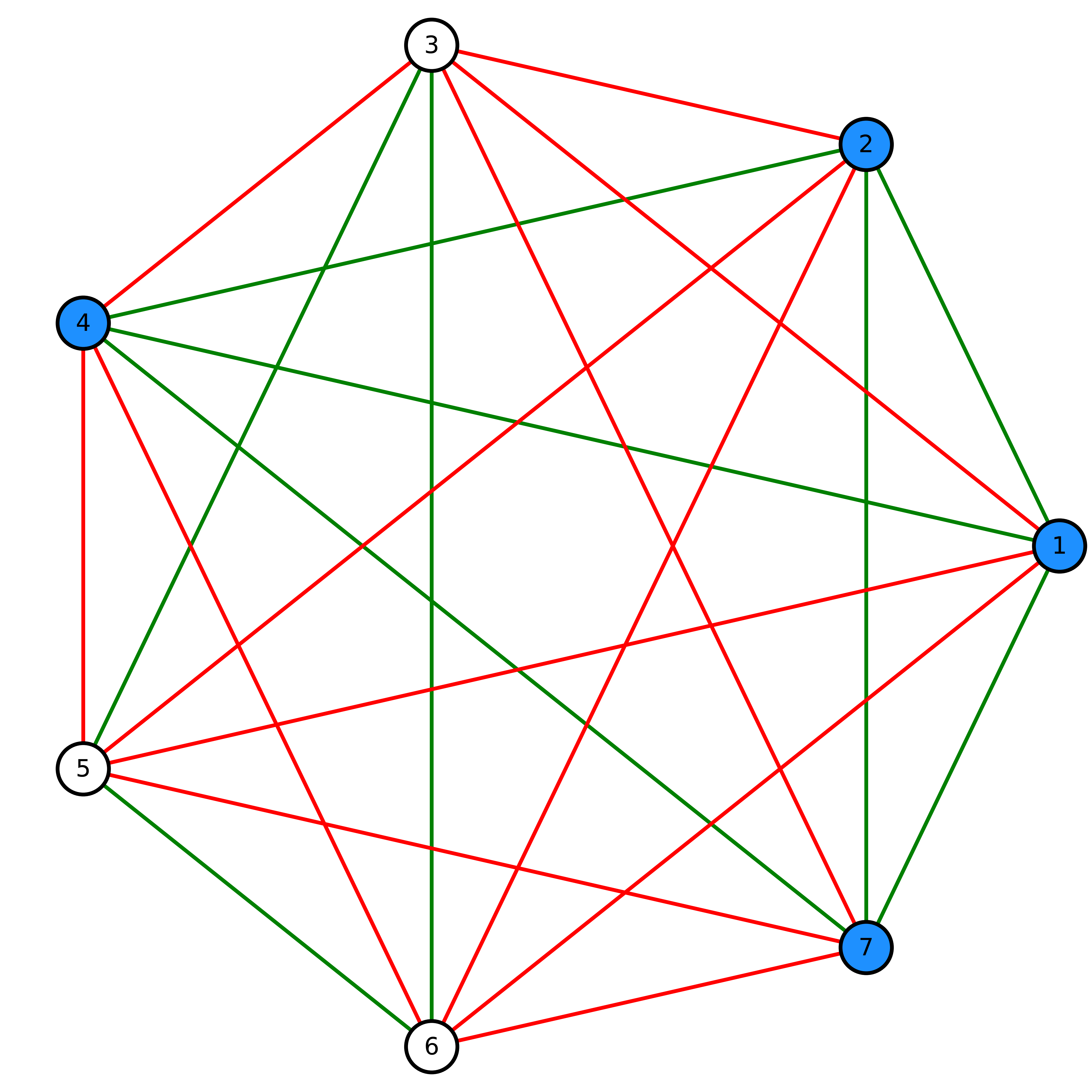
Figure 1: Network diagram for the example discussed. Blue vertices represent activated/firing neurons, whereas white vertices represent dormant/non-firing neurons. Green edges represent connections between neurons with the same state whereas red edges represent neuronal connections with opposite states.

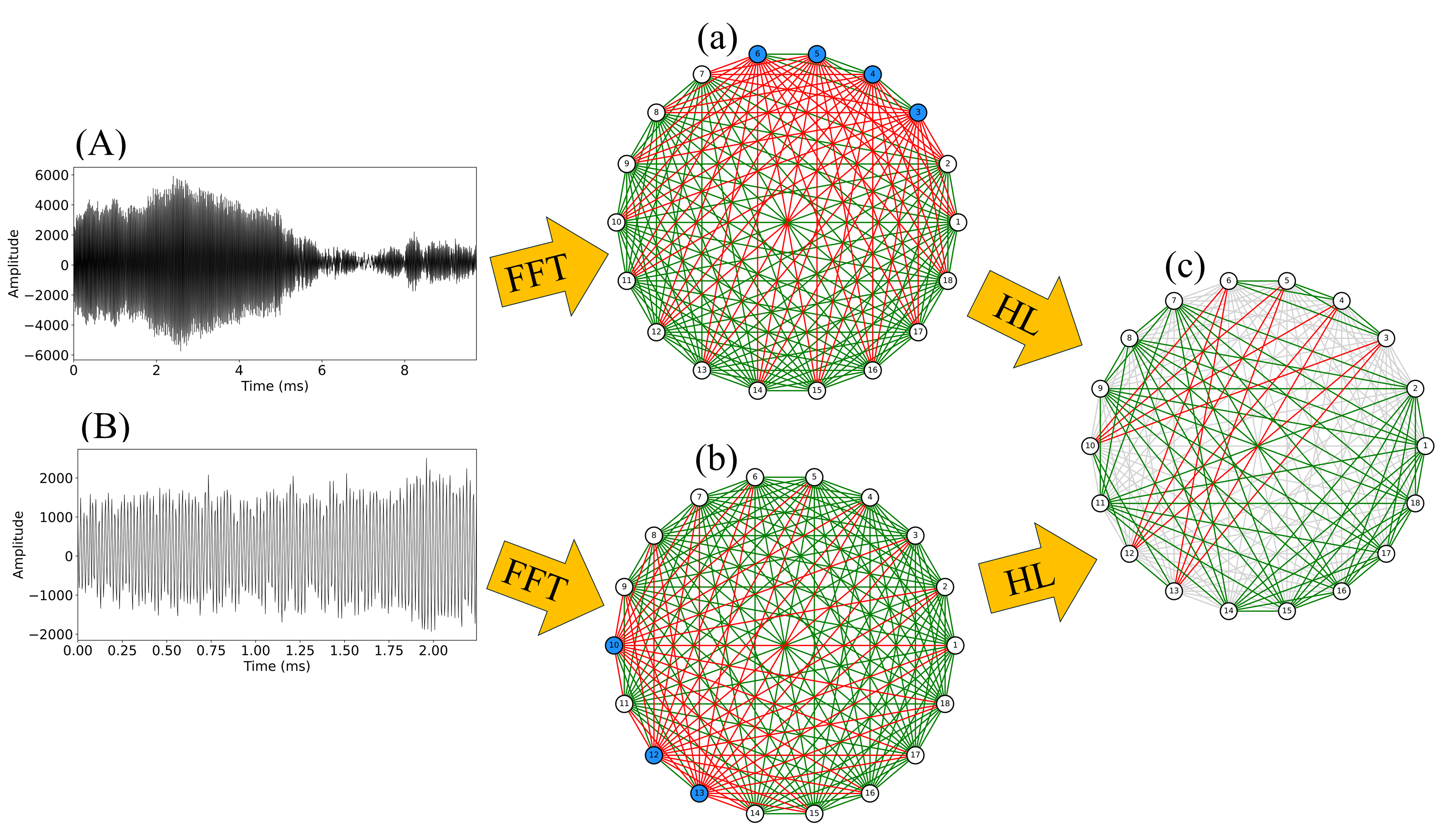
Figure 2: Fast Fourier Transform (FFT) is applied to the signals (A) and (B) which are the echolocation calls for each species PIPI and PIPY respectively. These are then used to activate the network, (a) and (b) respectively, where neurons which are fired are indicated in blue. In order for both of the echolocation calls to be stored in the network memory we combine the two network activations (a) and (b) using Hebbian learning (4) to form the trained network model (c), which is now ready for activation.

3.1 Hopfield Network Model

Hopfield networks are recurrent neural networks with associative memory patterns, and unlike the majority of neural network architectures used, such as feed-forward, Hopfield networks are fully connected (Hopfield, 1984). Hence, there are no separate input or output neurons. Instead the mean internal potential of the neuron is converted into a firing rate output of the neuron causing the network state to evolve with time. The classical Hopfield network for continuous variables can be described by the dynamical equations (Hopfield and Tank, 1985):

$$\frac{dy_{i}}{dt}=-\frac{y_{i}}{\tau}+\sum_{i}\sum_{j}w_{ij}x_{j}+I_{i}$$ (1)

where $\tau$ is a positive constant (resistance-capacitance); $y_{i}(t)$ is the internal state of the $i$-th neuron at time $t$; $x_{i}(t)$ is the activity of the $i$-th neuron at time $t$, $w_{ij}$ is the connection weight from neuron $j$ to neuron $i$; $I_{i}$ is the input bias of neuron $i$. In order to ensure convergence of the system to stable states where the output neurons, $x_{j}$, all remain constant we ensure the network connection weights, $w_{ij}$ are symmetric, i.e., $w_{ij}=w_{ji}$. If we also constrain the neurons to take on binary outputs, known as the high-gain limit, and there are no self-connections, $w_{ii}=0$, the system Lyapunov function, also known as “energy”, is given by:

$$E=-\frac{1}{2}\sum_{i}\sum_{j}w_{ij}x_{i}x_{j}-\sum_{i}I_{i}x_{i}$$ (2)

as described in Hopfield and Tank (1985). The stable states which the network converges to are the minima of this energy function. The state space of the network is the interior of the $N$-dimensional hypercube defined by $x_{i}=-1$ or $1$. In our formulation the minima occur at the corners of this hypercube.

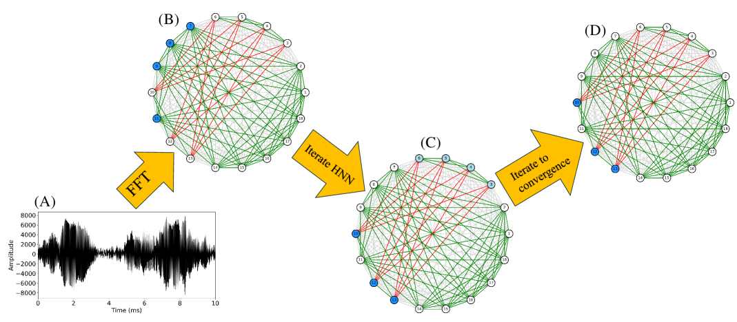
Figure 3: Fast Fourier Transform (FFT) is applied to the input signal (A) which may or may not contain echolocation calls for either species PIPI or PIPY. The FFT of the signal is then used to activate the trained network (B), where fired ($x_{i}=+1$) and non-fired ($x_{i}=-1$) neurons are blue and white respectively. The network then updates using equation 1 to form the next iteration of the HNN (C). Observe that in the second iteration (C), neutral neurons ($x_{i}=0$) are produced in light blue which are neither fired nor dormant. We continue to iterate the network until it converges which results in the final state of the network (D). We then compare the final state to the stored signals in the network memory, retrieval states (a) and (b) in figure 2. Hence, label this signal as either PIPI or PIPY if the final state is a retrieval state or label as UnID if the network converges to a spurious state.

The Hopfield network is of particular use to optimisation problems due to the guaranteed convergence of the network to local minima. In order to construct and apply a Hopfield network to a particular optimisation problem we must define the network weights $w_{ij}$. One method for assigning connection weights is to invoke Hebb’s rule or Hebbian learning (Hebb, 1949), the principle being “neurons that fire together, wire together”. Therefore, neurons that are active simultaneously become associated such that future activity in one will affect the activity of its associate neurons. In contrast, neurons that are not linked in this way, become less connected or associated. As an example for a network with $N=7$ neurons we will store a single network configuration given by $\mathbf{X}^{T}=[1,1,-1,1,-1,-1,1]$. The weights, $\mathbf{W}$, are computed via Hebb’s rule as follows:

$$\mathbf{W}=\mathbf{X}\cdot\mathbf{X}^{T}=\begin{bmatrix}1&1&-1&1&-1&-1&1\\ 1&1&-1&1&-1&-1&1\\ -1&-1&1&-1&1&1&-1\\ 1&1&-1&1&-1&-1&1\\ -1&-1&1&-1&1&1&-1\\ -1&-1&1&-1&1&1&-1\\ 1&1&-1&1&-1&-1&1\\ \end{bmatrix}$$ (3)

$\mathbf{X}$ in this example is known as a retrieval state (Hertz, 1991) and we represent this states network configuration in figure 1. In the case where multiple configurations are stored into the network we use the following formula to calculate the network weights:

$$\mathbf{W}=\frac{1}{N}\sum_{k=1}^{p}\mathbf{X}^{k}\cdot\mathbf{X}^{k}$$ (4)

where $p$ is the number of configurations stored in the network. Hopfield (1982) showed that “about $0.15N$ states can be simultaneously remembered before error in recall is severe”, hence we must be mindful of this constraint when constructing network architectures for successful memory recall. Also, it is possible for the Hopfield network to converge to states other than the retrieval states such as reversed states, mixture states and spin glass states (Hertz, 1991), these are known as spurious states.

3.2 Hopfield Network as a Bioacoustic Indentifier

We want our model network to be able to identify bat species based on their echolocation pulses, therefore we must represent these sound signals in the network. The issue we encounter is that, at their essence, signals are continuous and yet we wish to represent the signal within the network which is discrete. Therefore we take inspiration from biology, specifically the ear and brain. The ear and brain constitute a discretising listening, storage and recall device whereby continuous sound waves enter the ear as pressure perturbations which transduce in the middle ear into mechanical energy. These waves cause the tympanic membrane to vibrate, setting the ossicles (malleus, incus and stapes) in motion and in turn causing the oval window at the cochlea entrance to vibrate. This vibration causes the travelling wave to pass through the inner ear. The fluid filled cochlea is set in motion and a selection of the thousands of tiny auditory hair cells bend as the wave passes through the spiral, ultimately causing another transduction to electro-chemical neural impulses which transport information about the signal to the brain stem. The auditory hair cells act as biotransducers, discretising a continuous travelling wave into narrow bands of frequencies, characteristic of the location of the hair cell, high frequencies being detected first as the transformed waves enter the cochlea (Brownell, 1997; Dobie and Van Hemel, 2004). The coded discretised information about the sound waves is transmitted to the brain, relaying frequency, power, and temporal characteristics, and enabling a 3-dimensional acoustic representation of the world to be recreated.

The brain part of our model is represented by our Hopfield network (described in section 3.1), we just to need represent the ear aspect. For this we will use signal processing in order to digitise the signal ready for the network. The dataset which will be used to test the model is composed of 10384 1-dimensional wave files, hence the Fast Fourier transform (FFT) is a suitable algorithm to digitise such signals. Firstly we must train the model by selecting echolocation calls for each species from the dataset which are typical of those made by the respective species PIPI and PIPY. The FFT will convert the signal from the time domain into the frequency domain and peak frequencies are selected from each signal in order to activate the network. Using Hebbian learning these network configurations are stored in the network as retrieval states as described in figure 2. With our Hopfield network model constructed we use the remaining wave files in the dataset to test our model, which will attempt to identify them. In figure 3 we describe how signals are sent to the trained model (see figure 2) for prediction. An advantage of this algorithm is that we can easily observe how the network configuration evolves from one iteration to the next and therefore it is clear to understand how the model makes its predictions. Hence, the algorithm described here produces explainable AI models and therefore users can trust the results and outputs produced.

As outlined in section 3.1 it is possible the network does not converge to the retrieval states which correspond to the PIPI and PIPY echolocation calls the network was trained on, i.e., converge to spurious states of the network. This is in fact an advantage of this model since calls which are not identified as either PIPI or PIPY are labelled unidentified (UnID) by the model and can therefore be investigated separately.

4 Results

In this section we will present the results of the model (see section 3 on model construction) on the Bertran et al. (2019) dataset (see section 2 for information on the dataset). We try two versions of the model based on our insights about the dataset: Model $1$ is tested on the dataset after silences have been filtered out. Model $2$ is tested on the dataset after silences have been filtered out and also files of echolocation pulses with $\text{F}_{\text{maxE}}$ between $49$ and $51$ kHz removed (Russ, 2021; Aughney et al., 2018; Catto et al., 2003). Silences were filtered out automatically by determining whether the signal had any peak frequencies above a tunable tolerance before passing the remaining signals to the model. The algorithm was successful in identifying all silences before passing the remaining $8476$ files to the trained Hopfield network model for identification. Hence, the performance metrics only relate to the identification of PIPI and PIPY bat species and not on identifying the silences within the dataset, since this would over-inflate the metrics and give us an incorrect impression of performance with regard to identifying the two bat species based on echolocation calls.

Class	Model 1				Model 2
	Precision	Recall	F1	Support	Precision	Recall	F1	Support
PIPI	0.75	0.68	0.72	4193	0.79	0.84	0.81	2249
PIPY	0.72	0.76	0.74	4283	0.86	0.77	0.81	2550
	Overall Accuracy: $0.72$			$8476$	Overall Accuracy: $0.80$			4799

Table 1: Classification reports for model $1$ and $2$.

In table 1 and figure 4 we present the performance metrics and confusion matrix for both model $1$ and $2$. For model $1$ we observe an overall accuracy of $0.72$ with the highest metric being the $0.76$ recall score for the PIPY species which is very promising at this stage of model development. For model $2$ there is an increase in all performance metrics with an overall accuracy of $0.80$ with the highest performance metric of $0.86$ precision score for the PIPY species. For species surveying purposes, recall is of relevance to give accurate estimates of population size with model $2$ showing better performance for both PIPI and PIPY at $0.84$ and $0.77$ compared to model $1$. For other bioacoustic monitoring purposes, such as species specific interventions, precision would be the relevant metric with model $2$ showing better performance for both PIPI and PIPY at $0.79$ and $0.86$ compared to model $1$. The F1 score, the harmonic mean of precision and recall, shows better performance for Model $2$ with consistent scores for both PIPI and PIPY detection. The model performance is comparable to both commercial software (Marchal et al., 2022; Tabak et al., 2022) and the models developed by the dataset creators (Bertran et al., 2019). We will discuss the aspects of the data the model does not predict so well in section 5.

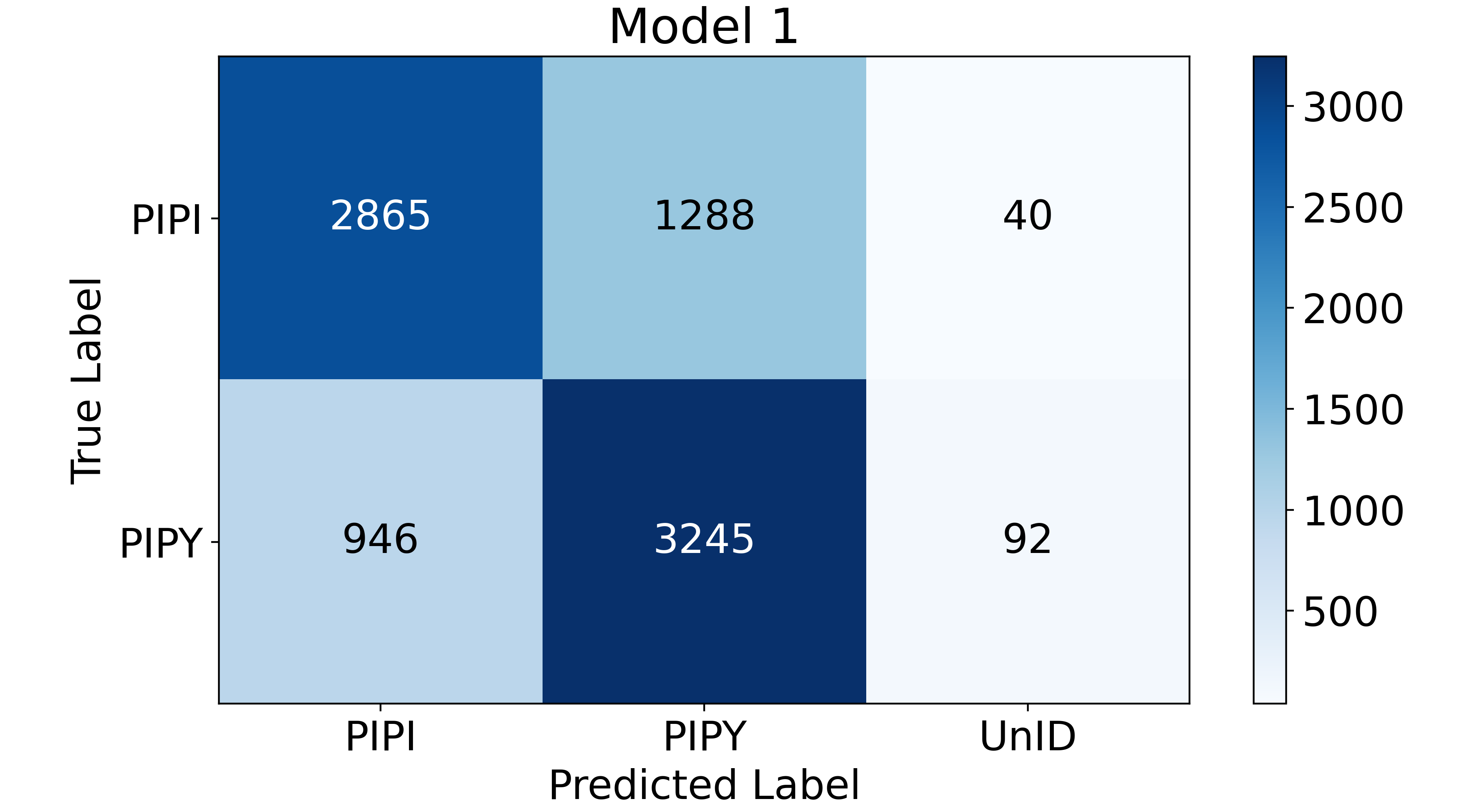
Figure 4: Confusion matrices for model $1$ and $2$.

The confusion matrix, in figure 4, gives us a breakdown of the model prediction compared to the true label given in the dataset. Note here we have an extra prediction label UnID, which the model returns when the neural network converges to a spurious state not associated with the training signals, as discussed in section 3. Essentially, for the signals labelled UnID, the model does not associate the signal with either of the PIPI or PIPY signals it was trained on. There are a total of $132$ signals in model $1$ and $104$ signals in model $2$ which are not identified as either PIPI or PIPY and hence need further investigation which we will discuss in section 5. We observe a marked decrease in the number of mislabelled PIPI signals predicted as PIPY by the model, from $1288$ in model $1$ to $322$ in model $2$. This infers that there are a large number of PIPI labelled signals in the dataset for which $\text{F}_{\text{maxE}}$ is between $49$ and $51$ kHz, which were removed from the dataset when testing model $2$ and hence improve the performance of model $2$ compared with model $1$. This is also true for the PIPY labelled signals in the dataset which where predicted as PIPI by the models.

Not only did model $2$ prove to be competitively accurate it also had low computational demands. It was developed and tested on a standard working laptop, an Apple MacBook Air. The model is fast, taking on average just $3$ milliseconds to train and only $5.4$ seconds to pre-process and classify all $10384$ publicly available bat recordings (Bertran Ferrer, 2019; Bertran et al., 2019). The model is also lightweight, i.e., it has a small average memory footprint of $144.09$ MB of RAM usage. To gain these average performance figures model $2$ was run five times in order to calculate the mean time taken and memory footprint. The laptop used was in normal use with other applications and tabs open and active.

5 Discussion

In this section we will discuss the results of the models, focusing on where the model did not agree with the dataset labelling of Bertran et al. (2019). These are given by the results in the four misclassified sets: PIPY detected as PIPI, PIPI detected as PIPY, PIPI detected as UnID and PIPY detected as UnID. The fully connected network architecture and iterative convergence process allows for interpretable classifications, as detailed in this section and described in figure 3, fulfilling the aim of being both transparent and explainable. We then go on to discuss further the computational performance of the model.

5.1 Dataset Limitations

Upon analysing the results of the two models in section 4 we notice three key issues which require discussion:

1. A large number of files ($3677$) had been labelled either PIPI or PIPY in the dataset even though the literature suggests that these signals should not be associated with either species (Russ, 2021; Catto et al., 2003).

2. Both models $1$ and $2$ returned $132$ and $104$ files respectively as unidentified results.

3. Although a small percentage overall, there were a total of $838$ mislabelled predictions made by model $2$; either PIPI identified as PIPY or PIPY identified as PIPI.

Figure 5: Full power spectral density plots comparing the species PIPI (red) and PIPY (green), which were stored in the neural network memory as retrieval states, with all of the cases of misclassified signals plotted in light blue for the indicated set. A typical example of a misclassified signal within the indicated set is shown in blue.

We have tried to account for point 1 by using two versions of the model: model $1$ and $2$ evaluated on the dataset with and without these $3677$ files included (see section 4) to compare performance. Not surprisingly we do see an improvement in the performance in model $2$ compared to model $1$. It is argued that these signals should not be considered echolocation calls from either PIPI or PIPY bat species and therefore we cannot expect the model to identify them.

Referring to point 2, the model developed here has a third class, ‘UnID’ (not present in the original dataset), which the model will return if the network converges to a spurious state not associated with either of the PIPI or PIPY echolocation calls stored in the network memory (retrieval states). These spurious states returned by the network are all reversed states, therefore not characteristic of either retrieval state. This is useful since the model will notify us when it does not recognise a signal as any stored within its memory and therefore we can immediately be made aware of unexpected and problematic recordings or potential model problems. This third class proved invaluable for initial result evaluation and understanding dataset limitations, and leveraged the network’s spurious states to express uncertainty.

In order to address point 3 (and point 2), and better understand how the model misclassified signals we plot the power spectral density of each of the four misclassified sets along with the original PIPI and PIPY species in figure 5. Using expert field guides and reports (Russ, 2021; Aughney et al., 2018; Catto et al., 2003) we can manually identify the calls to determine if we would classify these any differently to the model. Generally PIPI are considered identifiable if echolocating within the range of our model but below $48$ kHz, and PIPY identifiable if echolocation pulses are above $52$ kHz. In the top panels of figure 5 we would argue that our manual identification would agree with that of the model for the vast majority of signals and therefore disagree with the dataset labelling of these signals. In the bottom panels of figure 5, where the model returned ‘UnID’, these signals typically have frequencies either across the entire interval or inside the $49$ to $51$ kHz region. Hence, we would argue that the pattern of frequencies present in the power spectra is not distinct enough for ID as either pipistrelle species and these pulses were almost certainly not assigned correctly in the dataset.

We conclude that the overwhelming majority of the signals not detected correctly were either mislabelled in the original dataset or labelled despite expert consensus (Russ, 2021; Aughney et al., 2018; Catto et al., 2003); in isolation as single pulses these signals should not be considered indicative echolocation calls for these species. The call itself may not be species indicative for a variety of reasons: pipistrelles modifying their echolocation calls based on interaction with other bats, foraging or environmental factors. However, examination of the original file before the signals were split into single pulses, confirmed our mislabelling hypothesis.

5.2 Model Performance and Comparison

Model $2$ proves to be competitively accurate with an overall accuracy of $80$% as detailed in section 4 and also more importantly here has low computational demands. It was developed and tested on a standard working laptop, an Apple MacBook Air. The model proved to be extremely fast, taking on average just $3$ milliseconds to train and only $5.4$ seconds to pre-process and classify all $10384$ publicly available bat recordings (Bertran Ferrer, 2019; Bertran et al., 2019). Although the dataset creators Bertran et al. (2019) did develop a CNN with accuracy of $74$% for bat detection, computational demands were not discussed in their paper. On the laptop running our models we ran a short experiment to determine how long it would take to convert $10384$ sound files to spectrograms. Initially this was run through a Python IDE which crashed on every attempt. When run through the terminal, with low resolution spectrogram settings, the best we could manage was $6.5$ minutes to convert the files. In order to make these images suitable for a CNN, further processing would be required due to the irregular lengths of the WAV files within the dataset (Bertran Ferrer, 2019; Bertran et al., 2019). Creating these images took over $72$ times longer than our model takes to train, pre-process and classify all the files; recall our model processes the WAV files directly without the need to create spectrograms. Simply creating the spectrogram images takes $130000$ times longer than training our model, and indicates how costly the conversion to spectrograms is in CNN models. Not to mention the $14$ days to train CNNs from scratch when taking into account pretraining (You et al., 2018). Furthermore, local storage capacity is impacted as even these low resolution images result in over twice the amount of memory being used for storage prior to processing and classification. Our model is also lightweight, i.e., it has a small average memory footprint of $144.09$ MB of RAM usage. We should emphasise again here that this model can be built and run without requiring any access to high performance computing resources.

6 Conclusion

The model developed demonstrates the effectiveness of using associative memory as the training mechanism in order to detect bioacoustic events. This is advantageous due to the minimal training sets required which results in a fast and lightweight model trained in just $3$ milliseconds, pre-processing and classifying all $10384$ publicly available bat recordings in $5.4$ seconds. The model is lightweight since it is deployed on a standard working laptop (Apple MacBook Air) and has a small average memory footprint ($144.09$ MB of RAM usage). This is in stark contrast to the CNN approach more commonly used which requires vast amounts of labelled training data and signifcant computational resources (GPUs, high performance computing resources etc.). These types of models are ideal for bioacoustic monitoring given the vast amounts of unlabelled data collected (limited training data), importance of rare species detection and limited resources in the field. We have shown that the model is competitively accurate, assisting in essential problem solving within the field of conservation. The model’s low energy, time and hardware requirements mean that its use is sustainable and fits well with conservation, ecology and equitable AI long term goals.

A further advantage of using an HNN is that the model is inherently interpretable. We can dig into each classification and discover exactly how it was made, see figure 3. This transparency and explainability was particularly advantageous, when evaluating the model performance. At this point we became aware of the limitations of the dataset: principally the inclusion and labelling of calls which are widely agreed to be inappropriate for classification; and the mislabelling of a significant proportion of files. Hence, although the dataset and the classification task, were chosen in order to best introduce and demonstrate a novel algorithm to building AI models in the field of bioacoustics, the performance metrics do not tell the whole story. In fact, with further analysis of the results, it was hard to find any examples of disagreement between model and manual identification using expert field guides. It should be stressed that the model was not designed to classify species but to detect similar signals within its memory. We train the model on species specific echolocation calls and from this we infer the species of bat. Hence, models can therefore be constructed to detect different species or particular vocalisations.

Biologically inspired mathematical models, such as these associative memory HNNs, have great potential to assist with modern problems, but as we have outlined here the current emphasis amongst Global North researchers is on large training datasets, heavyweight convolutional neural networks and large language models. We suggest that brain-inspired lightweight associative memory models offer a sustainable and equitable way forward as we move into an era where reducing human environmental impact is critical to the survival of all species on a warming planet.

7 Acknowledgements

We thank the OpenBright Foundation and trustee Elizabeth Molyneux for their support and funding. We also thank the University of Wolverhampton for the Invest to Grow PhD Studentship funding. The authors would also like to thank Catherine Povey (Just Mammals Ltd) for her expertise and useful discussions.

References

- Abrahams and Geary (2020) Abrahams, C., Geary, M., 2020. Combining bioacoustics and occupancy modelling for improved monitoring of rare breeding bird populations. Ecological Indicators 112. doi:10.1016/j.ecolind.2020.106131.
- Apodemus Field Equipment (2025) Apodemus Field Equipment, 2025. Apodemus pippyg. https://www.apodemus.eu/en/Apodemus-Pippyg/00127. Accessed: 2025-04-04.
- Aughney et al. (2018) Aughney, T., Roche, N., Langton, S., 2018. The Irish Bat Monitoring Programme 2015-2017. Irish Wildlife Manuals, No. 103, National Parks and Wildlife Service. Department of Culture, Heritage and the Gaeltacht, Ireland.
- Bakker (2022) Bakker, K., 2022. The Sounds of Life: How Digital Technology is Bringing Us Closer to the Worlds of Animals and Plants. Princeton, NY: Princeton University Press.
- Barlow and Jones (1999) Barlow, K., Jones, G., 1999. Roosts, echolocation calls and wing morphology of two phonic types of pipistrellus pipistrellus. International Journal of Mammalian Biology 64, 257–268.
- Bertran et al. (2019) Bertran, M., Alsina-Pagès, R., Tena, E., 2019. Pipistrellus pipistrellus and pipistrellus pygmaeus in the iberian peninsula: An annotated segmented dataset and a proof of concept of a classifier in a real environment. Applied Sciences 9. doi:10.3390/app9173467.
- Bertran Ferrer (2019) Bertran Ferrer, M., 2019. Bat recordings split data set. Zenodo doi:10.1038/s41598-023-49989-z.
- Bouza et al. (2023) Bouza, L., Bugeau, A., Lannelongue, L., 2023. How to estimate carbon footprint when training deep learning models? a guide and review. Environmental Research Communications 5, 115014. URL: https://dx.doi.org/10.1088/2515-7620/acf81b, doi:10.1088/2515-7620/acf81b.
- Bradfer-Lawrence et al. (2023) Bradfer-Lawrence, T., Desjonqueres, C., Eldridge, A., Johnston, A., Metcalf, O., 2023. Using acoustic indices in ecology: Guidance on study design, analyses and interpretation. Methods in Ecology and Evolution 14 (9), 2192–2204. doi:10.1111/2041-210X.14194.
- Brownell (1997) Brownell, W., 1997. How the ear works - nature’s solutions for listening. Volta Rev 99 (5). doi:PMC2888317.
- Catto et al. (2003) Catto, C., Coyte, A., Agate, J., Langton, S., 2003. Bats as Indicators of Environmental Quality R&D Technical Report E1-129/TR. Technical Report ISBN: 1 844 32251 3. Environment Agency. Rio House, Waterside Drive, Aztec West, Almondsbury Bristol BS32 4UD. N.B. This document was produced under R&D Project E1-129 by the Bat Conservation Trust.
- Chen et al. (2019) Chen, C., Li, O., Tao, C., Barnett, A., Su, J., Rudin, C., 2019. This looks like that: Deep learning for interpretable image recognition. URL: https://arxiv.org/abs/1806.10574, arXiv:1806.10574.
- Chen and Aihara (1995) Chen, L., Aihara, K., 1995. Chaotic simulated annealing by a neural network model with transient chaos. Neural Networks 8, 915–930. doi:10.1016/0893-6080(95)00033-V.
- Dai and Nakano (1998) Dai, Y., Nakano, Y., 1998. Recognition of facial images with low resolution using a hopfield memory model. Pattern Recognition 31 (2), 159–167. doi:10.1016/S0031-3203(97)00040-X.
- Dobie and Van Hemel (2004) Dobie, R., Van Hemel, S., 2004. Hearing Loss: Determining Eligibility for Social Security Benefits. National Academies Press (US). chapter 2. pp. 42–68. doi:10.17226/11099.
- Dosovitskiy et al. (2020) Dosovitskiy, A., Beyer, L., Kolesnikov, A., Weissenborn, D., Zhai, X., Unterthiner, T., Dehghani, M., Minderer, M., Heigold, G., Gelly, S., Uszkoreit, J., Houlsby, N., 2020. An image is worth 16x16 words: Transformers for image recognition at scale. CoRR abs/2010.11929. URL: https://arxiv.org/abs/2010.11929.
- Dufourq et al. (2022) Dufourq, E., Batist, C., Foquet, R., Durbach, I., 2022. Passive acoustic monitoring of animal populations with transfer learning. Ecological Informatics 70, 101688. doi:10.1016/j.ecoinf.2022.101688.
- Ferreira et al. (2025) Ferreira, A., Felipe da Silva, N., Mesquita, F., Rosa, T., Buchmann, S., Mesquita-Neto, J., 2025. Transformer models improve the acoustic recognition of buzz-pollinating bee species. Ecological Informatics 86, 103010. doi:10.1016/j.ecoinf.2025.103010.
- Funosas et al. (2024) Funosas, D., Barbaro, L., Schillé, L., Elger, A., Castagneyrol, B., Cauchoix, M., 2024. Assessing the potential of birdnet to infer european bird communities from large-scale ecoacoustic data. Ecological Indicators 164, 112146. doi:10.1016/j.ecolind.2024.112146.
- Ghani et al. (2023) Ghani, B., Denton, T., Kahl, S., Klinck, H., 2023. Global birdsong embeddings enable superior transfer learning for bioacoustic classification. Scientific Reports 13, 22876. doi:10.1038/s41598-023-49989-z.
- Goodwin and Gillam (2021) Goodwin, K., Gillam, E., 2021. Testing accuracy and agreement among multiple versions of automated bat call classification software. Wildlife Society Bulletin 45, 690–705. doi:10.1002/wsb.1235.
- Hebb (1949) Hebb, D., 1949. The Organization of Behavior: A Neuropsychological Theory, 1st ed. Wiley.
- Heinrich et al. (2025) Heinrich, R., Rauch, L., Sick, B., Scholz, C., 2025. Audioprotopnet: An interpretable deep learning model for bird sound classification. Ecological Informatics 87, 103081. doi:10.1016/j.ecoinf.2025.103081.
- Hertz (1991) Hertz, J., 1991. Introduction To The Theory Of Neural Computation (1st ed.). CRC Press. doi:10.1201/9780429499661.
- Hill et al. (2019) Hill, A., Prince, P., Snaddon, J., Doncaster, C., Rogers, A., 2019. Audiomoth: A low-cost acoustic device for monitoring biodiversity and the environment. HardwareX 6, e00073. doi:10.1016/j.ohx.2019.e00073.
- Hopfield (1982) Hopfield, J., 1982. Neural networks and physical systems with emergent collective computational abilities. Proceedings of the National Academy of Sciences, USA 79, 2554–2558. doi:10.1073/pnas.79.8.2554.
- Hopfield (1984) Hopfield, J., 1984. Neurons with graded response have collective computational properties like those of two-state neurons. Proceedings of the National Academy of Sciences of the United States of America 81 (10), 3088–3092. doi:10.1073/pnas.81.10.3088.
- Hopfield and Tank (1985) Hopfield, J., Tank, D., 1985. ”neural” computation of decisions in optimization problems. Biological cybernetics 52, 141–152. doi:10.1007/BF00339943.
- Kahl et al. (2021) Kahl, S., Wood, C., Eibl, M., Klinck, H., 2021. Birdnet: A deep learning solution for avian diversity monitoring. Ecological Informatics 61, 101236. doi:10.1016/j.ecoinf.2021.101236.
- Kershenbaum et al. (2025) Kershenbaum, A., Akçay, Ç., Babu-Saheer, L., Barnhill, A., Best, P., Cauzinille, J., Clink, D., Dassow, A., Dufourq, E., Growcott, J., Markham, A., Marti-Domken, B., Marxer, R., Muir, J., Reynolds, S., Root-Gutteridge, H., Sadhukhan, S., Schindler, L., Smith, B., Stowell, D., Wascher, C., Dunn, J., 2025. Automatic detection for bioacoustic research: a practical guide from and for biologists and computer scientists. Biological Reviews 100, 620–646. doi:10.1111/brv.13155.
- Liu et al. (2023) Liu, S., Gao, X., Chen, L., Zhou, S., Peng, Y., Yu, D., Ma, X., Wang, Y., 2023. Multi-traveler salesman problem for unmanned vehicles: Optimization through improved hopfield neural network. Sustainability 15. doi:10.3390/su152015118.
- Liu et al. (2022) Liu, Z., Mao, H., Wu, C., Feichtenhofer, C., Darrell, T., Xie, S., 2022. A convnet for the 2020s. URL: https://arxiv.org/abs/2201.03545, arXiv:2201.03545.
- Mac Aodha et al. (2018) Mac Aodha, O., Gibb, R., Barlow, K., Browning, E., Firman, M., Freeman et al, R., 2018. Bat detective—deep learning tools for bat acoustic signal detection. PLOS Computational Biology 14 (3), e1005995. doi:10.1371/journal.pcbi.1005995.
- MacIsaac et al. (2024) MacIsaac, J., Newson, S., Ashton-Butt, A., Pearce, H., Milner, B., 2024. Improving acoustic species identification using data augmentation within a deep learning framework. Ecological Informatics 83, 102851. doi:10.1016/j.ecoinf.2024.102851.
- Manzano-Rubio et al. (2022) Manzano-Rubio, R., Bota, G., Brotons, L., Soto-Largo, E., Pérez-Granados, C., 2022. Low-cost open-source recorders and ready-to-use machine learning approaches provide effective monitoring of threatened species. Ecological Informatics 72, 101910. doi:10.1016/j.ecoinf.2022.101910.
- Marchal et al. (2022) Marchal, J., Fabianek, F., Aubry, Y., 2022. Software performance for the automated identification of bird vocalisations: the case of two closely related species. Bioacoustics 31 (4), 397–413. doi:10.1080/09524622.2021.1945952.
- McEwen et al. (2024) McEwen, B., Soltero, K., Gutschmidt, S., Bainbridge-Smith, A., Atlas, J., Green, R., 2024. Active few-shot learning for rare bioacoustic feature annotation. Ecological Informatics 82, 102734. doi:10.1016/j.ecoinf.2024.102734.
- Metcalf et al. (2023) Metcalf, O., Abrahams, C., Ashington, B., Baker, E., Bradfer-Lawrence, T., Browning, E., Carruthers-Jones, J., Darby, J., Dick, J., Eldridge, A., Elliott, D., Heath, B., Howden-Leach, P., Johnston, A., Lees, A., Meyer, C., Ruiz Arana, U., Smyth, S., 2023. Good practice guidelines for long-term ecoacoustic monitoring in the UK. Technical Report. The UK Acoustics Network. URL: https://e-space.mmu.ac.uk/631466/1/Good_practice_guidelines_for_long-term%20%281%29.pdf.
- Mydlarz et al. (2017) Mydlarz, C., Salamon, J., Bello, J., 2017. The implementation of low-cost urban acoustic monitoring devices. Applied Acoustics 117, 207–218. doi:10.1016/j.apacoust.2016.06.010. acoustics in Smart Cities.
- NobelPrize.org (2024) NobelPrize.org, 2024. The nobel prize in physics 2024. https://www.nobelprize.org/uploads/2024/11/press-physicsprize2024-2.pdf. Accessed: 2025-04-04.
- Northcutt et al. (2021) Northcutt, C., Athalye, A., Mueller, J., 2021. Pervasive label errors in test sets destabilize machine learning benchmarks. URL: https://arxiv.org/abs/2103.14749, arXiv:2103.14749.
- Pierce and Griffin (1938) Pierce, G., Griffin, D., 1938. Experimental determination of supersonic notes emitted by bats. Journal of Mammalogy 19 (4), 454–455. doi:10.2307/1374231.
- Planque, B. (2024) Planque, B. , 2024. A short introduction to machine learning results. https://xeno-canto.org/article/299. Accessed: 2025-04-04.
- Pérez-Granados (2023) Pérez-Granados, C., 2023. Birdnet: applications, performance, pitfalls and future opportunities. Ibis 165, 1068–1075. doi:10.1111/ibi.13193.
- Pérez-Granados and Traba (2021) Pérez-Granados, C., Traba, J., 2021. Estimating bird density using passive acoustic monitoring: a review of methods and suggestions for further research. Ibis 163, 765–783. doi:10.1111/ibi.12944.
- Rasmussen et al. (2024) Rasmussen, J., Stowell, D., Briefer, E., 2024. Sound evidence for biodiversity monitoring. Science 385, 138–140. doi:10.1126/science.adh2716.
- Rodden et al. (2024) Rodden, E., Gascoyne, A., Naughton, L., Brennan, J., Parkes, A., 2024. Transient chaotic neural network with negative self-feedback memory for continuous optimisation problems, in: Arai, K. (Ed.), Proceedings of the Future Technologies Conference (FTC) 2024, Volume 1, Springer Nature Switzerland, Cham. pp. 290–303.
- Russ (2021) Russ, J., 2021. Bat calls of Britain and Europe. Bat Biology and Conservation, Pelagic Publishing, Exeter, England.
- Salem et al. (2024) Salem, S., Shirayama, S., Shimazaki, S., Oki, K., 2024. Ensemble deep learning and anomaly detection framework for automatic audio classification: Insights into deer vocalizations. Ecological Informatics 84, 102883. doi:10.1016/j.ecoinf.2024.102883.
- Sandbrook (2025) Sandbrook, C., 2025. Beyond the hype: Navigating the conservation implications of artificial intelligence. Conservation Letters 18, e13076. doi:10.1111/conl.13076.
- Sethi et al. (2022) Sethi, S., Kovac, M., Wiesemüller, F., Miriyev, A., Boutry, C., 2022. Biodegradable sensors are ready to transform autonomous ecological monitoring. Nature Ecology and Evolution 6, 1245–1247. doi:10.1038/s41559-022-01824-w.
- Stowell (2022) Stowell, D., 2022. Computational bioacoustics with deep learning: a review and roadmap. PeerJ 10, e13152. doi:10.7717/peerj.13152.
- Szesciorka et al. (2023) Szesciorka, A., McCullough, L.K., Oleson, E., 2023. An unknown nocturnal call type in the mariana archipelago. JASA Express Lett 3 (1), 011201. doi:10.1121/10.0017068.
- Tabak et al. (2022) Tabak, M., Murray, K., Reed, A., Lombardi, J., Bay, K., 2022. Automated classification of bat echolocation call recordings with artificial intelligence. Ecological Informatics 68, 101526. doi:10.1016/j.ecoinf.2021.101526.
- Teixeira et al. (2019) Teixeira, D., Maron, M., van Rensburg, B., 2019. Bioacoustic monitoring of animal vocal behavior for conservation. Conservation Science and Practice 1 (8). doi:10.1111/csp2.72.
- Thompson et al. (2021) Thompson, N.C., Greenewald, K., Lee, K., Manso, G.F., 2021. Deep learning’s diminishing returns: The cost of improvement is becoming unsustainable. IEEE Spectrum 58, 50–55. doi:10.1109/MSPEC.2021.9563954.
- Toews, R. (2020) Toews, R. , 2020. Deep learning’s carbon emissions problem. https://www.forbes.com/sites/robtoews/2020/06/17/deep-learnings-climate-change-problem/. Accessed: 2025-04-04.
- Wildlife Acoustics (2017) Wildlife Acoustics, 2017. Kaleidoscope pro bat auto id how it works. https://vimeo.com/182997396. Accessed: 2025-04-04.
- Wildlife Acoustics (2024) Wildlife Acoustics, 2024. Products. https://www.wildlifeacoustics.com/products. Accessed: 2025-04-04.
- Yoh et al. (2022) Yoh, N., Kingston, T., McArthur, E., Aylen, O., Huang, J., Jinggong, E., Khan, F., Lee, B., Mitchell, S., Bicknell, J., Struebig, M., 2022. A machine learning framework to classify southeast asian echolocating bats. Ecological Indicators 136, 108696. doi:10.1016/j.ecolind.2022.108696.
- You et al. (2018) You, Y., Zhang, Z., Hsieh, C.J., Demmel, J., Keutzer, K., 2018. Imagenet training in minutes. URL: https://arxiv.org/abs/1709.05011, arXiv:1709.05011.