Search for pseudoscalar Higgs boson $A_{0}$ of the Bestest Little Higgs model at the LHC and FCC-hh

Abstract

We analyse the sensitivity of the Large Hadron Collider (LHC) and the Future Circular Collider-hadron-hadron (FCC-hh) to the existence of pseudoscalar Higgs boson $A_{0}$ predicted by the Bestest Little Higgs model. We study the tree-level (two and three body) and one-loop decays of the pseudoscalar, $A_{0}\to b\bar{b},t\bar{t},\gamma t\bar{t},\gamma b\bar{b},Zt\bar{t},Zb\bar{b},Wt\bar{b},h_{0}t\bar{t},h_{0}b\bar{b}$, and $A_{0}\to\gamma\gamma,\gamma Z,ZZ,gg,WW$, respectively. In addition, we perform a phenomenological study of the production of the pseudoscalar $A_{0}$ via gluon fusion $gg\to A_{0}\to Y$ processes, where $Y\equiv\gamma\gamma,\gamma Z,ZZ,gg,WW$. From the cross section of the processes of interest and the expected integrated luminosity of the LHC and FCC-hh, we determined the number of events that could be produced in both colliders.

I Introduction

The discovery of a Higgs boson with a mass of 125 GeV by the ATLAS ATLAS:2012yve and CMS CMS:2012qbp collaborations at the CERN LHC has motivated the search for new exotic states at current and future colliders. Another significant fact is the recent observation of the production of four top quarks in proton-proton collisions at a center-of-mass energy of 13 TeV CMS:2023ftu ; ATLAS:2023ajo . This is one of the rarest processes in the Standard Model (SM) that is currently accessible at hadron colliders. The top quark, the heaviest elementary particle in the SM, has strong connections to the SM Higgs boson and new particles predicted in theories beyond the SM (BSM). Many of these new heavy particles can decay into top quarks, resulting in the production of four top quarks via intermediate exotic particles. Such a signature could indicate the existence of new BSM particles.

The unsolved puzzles of the SM (such as dark energy, dark matter, neutrino masses, and the matter-antimatter asymmetry, among others) require new BSM physics. Many of these theories necessitate a richer Higgs sector. This extended sector is a common feature of several extended models. The Higgs sector itself has become a fundamental tool in the search for new physics, which could manifest in various ways. For example, the discovery of additional Higgs bosons or the measurement of new sources of CP violation in the scalar sector would provide direct evidence of BSM physics Englert:2014uua . So far, both direct and indirect searches for new physics have produced unsuccessful results. However, it is expected that the scope of these searches will expand considerably in the future, as colliders will operate at such high energy scales that new signal channels will open up which would be suppressed at lower energies. The discovery of new non-SM Higgs bosons would be a clear sign of BSM physics with extended sectors.

Several extended models have been proposed to address open issues in the SM scenario, such as the hierarchy problem Schmaltz:2002wx . This problem is also known as the fine-tuning problem. Among the BSM models, there are Little Higgs-type models Arkani-Hamed:2002ikv ; Chang:2003zn ; Han:2003wu ; Chang:2003un ; Schmaltz:2004de that introduce enough new physics to generate cancellations and preserve a light Higgs boson. These models implement the idea that the Higgs boson is a pseudo-Goldstone boson. Little Higgs theories are constructed by embedding the SM within a larger group with an extended symmetry. From a phenomenological point of view, this symmetry requires the existence of new particles whose couplings ensure that large contributions to the Higgs mass cancel out. Thus, the Higgs boson mass is protected from radiative corrections. Although Little Higgs models offer an attractive solution to the hierarchy problem, many of them exhibit certain theoretical inconsistencies Schmaltz:2008vd . For example, the mechanism used to generate a Higgs quartic coupling leads to violations of custodial symmetry. They are also strongly constrained by electroweak precision data in the gauge sector.

The Bestest Little Higgs model (BLHM) JHEP09-2010 ; Godfrey:2012tf ; Kalyniak:2013eva was formulated to resolve the theoretical inconsistencies found in most Little Higgs theories. This model introduces separate symmetry-breaking scales, $f$ and $F$, where $F>f$. In this way, the new heavy quarks ($T$, $T_{5}$, $T_{6}$, $T^{2/3}$, $T^{5/3}$, $B$) acquire masses proportional to the $f$ scale, while the new gauge bosons ($Z^{\prime}$, $W^{\prime\pm}$) acquire masses proportional to a combination of the $f$ and $F$ scales. These gauge boson partners allow the model to evade the constraints imposed by electroweak precision measurements. A successful quartic Higgs coupling is also generated without introducing any dangerous singlet in the scalar sector Schmaltz:2008vd , in contrast to other Little Higgs models. Instead, an additional singlet (satisfying certain additional symmetries) and a custodial $SU(2)$ symmetry JHEP09-2010 . The scalar sector of the BLHM has a rich phenomenology that generates neutral and charged scalar fields: $h_{0},H_{0},A_{0},\phi^{0},\eta^{0},H^{\pm},\phi^{\pm}$, and $\eta^{\pm}$. We recommend that interested readers refer to Refs. Martinez-Martinez:2024lez ; Cruz-Albaro:2024vjk ; Cruz-Albaro:2022lks for more information on the BLHM.

In this work, we investigate the production of the pseudoscalar Higgs boson $A_{0}$ via gluon fusion at current and future colliders, such as the LHC ZurbanoFernandez:2020cco ; Azzi:2019yne ; Cepeda:2019klc ; FCC:2018bvk and the FCC-hh MammenAbraham:2024gun ; Mangano:2022ukr ; FCC:2018byv ; FCC:2018vvp . Specifically, we discuss searching for pseudoscalar $A_{0}$ decays into gauge bosons ($VV$, where $V=\gamma,Z,W,g$) within the context of the BLHM. Although $A_{0}\to VV$ decay is an induced process at one-loop level, we believe the pseudoscalar could be first detected in a two-photon final state, similar to the discovery of the SM Higgs boson ATLAS:2012ad ; CMS:2012qbp ; ATLAS:2015yey . Searches in the di-photon channel are especially useful as it offers the best mass resolution and an exceptionally clean signal because the CMS and ATLAS detectors reconstruct photons with high precision. However, even if the pseudoscalar Higgs $A_{0}$ is discovered in other final states, the other possible decays must be confirmed or excluded. Thus, this study will provide information about the BLHM and the potential detection of the pseudoscalar $A_{0}$ at the LHC and the future 100 TeV collider.

The physics programs of current and future hadron, lepton, and hybrid colliders include, among their research objectives, the theoretical, phenomenological, and experimental study of exotic particles, such as the pseudoscalar $A_{0}$ predicted by several extensions of the SM. One of these extensions is the BLHM. For further information on studies of the pseudoscalar within other BSM frameworks, we recommend that interested readers consult Refs. Arhrib:2018pdi ; Abu-Ajamieh:2025zcv ; Aranda:2017bgq . On the other hand, experimental searches for pseudoscalar Higgs bosons are essential, as they provide complementary information to theoretical predictions and help constrain the parameter space of BSM models Cornell:2020usb ; Almarashi:2021pgu . Some searches for the pseudoscalar have been conducted in proton-proton collisions at center-of-mass energies of 8 and 13 TeV with the ATLAS detector, where the pseudoscalar $A_{0}$ is produced in association with a top quark pair, followed by the decay $A_{0}\to t\bar{t}$ (i.e., $t\bar{t}A_{0}\to t\bar{t}t\bar{t}$) ATLAS:2024jja ; ATLAS:2022rws ; ATLAS:2017snw . Another possible production mechanism for the pseudoscalar occurs in association with a $Z$ gauge boson via gluon fusion at the LHC ($gg\to ZA_{0}\to l\bar{l}b\bar{b}+X$) Kao:2003jw . The results of these search channels have been interpreted within the framework of the Two-Higgs Doublet model (2HDM); however, they can also be investigated within the BLHM scenario. These studies are currently underway, and we expect to publish the results soon. These different discovery channels offer valuable opportunities to search for the pseudoscalar both at the LHC and at future colliders and may provide new insights into BSM physics.

The article is organized as follows. In Section II, we present the analytical calculations of the tree-level and one-loop decays of the pseudoscalar Higgs boson $A_{0}$. In Section III, the numerical results are discussed. Finally, conclusions are presented in Section IV. The effective couplings involved in our calculations are provided in Appendix A.

II Pseudoscalar $A_{0}$ decays in the BLHM

In this section, we determine the partial decay widths of the pseudoscalar $A_{0}$, or otherwise provide the corresponding transition amplitudes. In this regard, we will consider direct search channels with final states of the SM. In the following, we describe the different decay modes of the Higgs boson pseudoscalar $A_{0}$.

II.1 Two-body decays at tree level

The Feynman diagrams corresponding to the tree-level two-body decays of the pseudoscalar $A_{0}$ are shown in Fig. 1. To obtain the analytical expressions for the decay widths, we use the Feynman rules for the interaction vertices as given in Refs. Cruz-Albaro:2022lks ; Cruz-Albaro:2023pah ; Cruz-Albaro:2022kty ; Gutierrez-Rodriguez:2023sxg , with the corresponding effective couplings detailed in Appendix A. Next, in Eqs. (1) and (2) we provide the resulting expressions for the partial decay widths

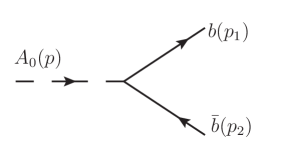
Figure 1: Feynman diagrams corresponding to the tree-level two-body decays of the pseudoscalar $A_{0}$.

$$\Gamma(A_{0}\to t\bar{t}) = \frac{N_{C}\,g_{A_{0}tt}^{2}m_{A_{0}}}{8\pi}\left(1-\frac{4m_{t}^{2}}{m_{A_{0}}^{2}}\right)^{1/2},$$ (1)

$$\Gamma(A_{0}\to b\bar{b}) = \frac{N_{C}\,g_{A_{0}bb}^{2}m_{A_{0}}}{8\pi}\left(1-\frac{4m_{b}^{2}}{m_{A_{0}}^{2}}\right)^{1/2}.$$ (2)

The colour factor of the quarks is represented by $N_{C}$ in these expressions, while the effective couplings are denoted by $g_{A_{0}tt}$ and $g_{A_{0}bb}$ (see Appendix A).

II.2 Three-body decays at tree level

Tree-level three-body decays are fundamental processes in particle physics, as they correspond to the leading-order contributions in the perturbative expansion and can yield significant effects in various scenarios. In the context of the BLHM, the Feynman diagrams corresponding to the three-body decays of the pseudoscalar $A_{0}$ are shown in Fig. 2. For these processes, we provide only the decay amplitudes, since the analytical expressions for the decay widths are typically very lengthy. Moreover, the associated phase space is more complex, involving non-trivial multidimensional integrations. The analytical expressions for the decay amplitudes are calculated using the generic formula described in Eq. (3) pdg:2023 ; Barger:1996 ; Barradas:1996xb :

$$\frac{d\Gamma(A_{0}\to ABC)}{dx_{a}dx_{b}}=\frac{m_{A_{0}}}{256\,\pi^{3}}|\mathcal{M}(A_{0}\to ABC)|^{2}.$$ (3)

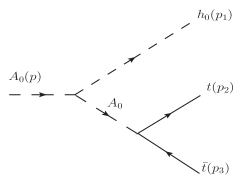
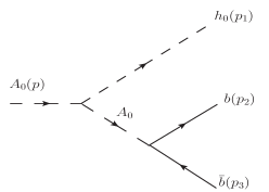
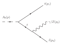
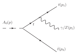
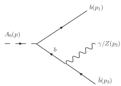
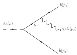
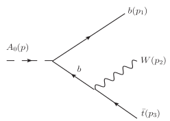
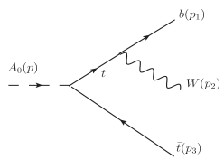
Figure 2: Feynman diagrams corresponding to the tree-level three-body decays of the pseudoscalar $A_{0}$.

From the Feynman diagrams (see Fig. 2), we derive the following generic amplitudes:

$$\mathcal{M}(A_{0}\to h_{0}q_{i}\bar{q}_{i})= g_{A_{0}A_{0}h_{0}}g_{A_{0}q_{i}q_{i}}\left(\frac{i}{k^{2}-m^{2}_{A_{0}}}\right)\bar{u}(p_{2})\gamma^{5}v(p_{3}),$$ (4)

$$\mathcal{M}(A_{0}\to\gamma q_{i}\bar{q}_{i}) = g_{A_{0}q_{i}q_{i}}g_{\gamma q_{i}q_{i}}\bigg{[}\bar{u}(p_{1})\gamma^{5}\left(\frac{i(-\not{k}+m_{q_{i}})}{k^{2}-m^{2}_{q_{i}}}\right)\gamma^{\mu}v(p_{3})$$ (5)

$$+ \bar{u}(p_{1})\gamma^{\mu}\left(\frac{i(\not{k}+m_{q_{i}})}{k^{2}-m^{2}_{q_{i}}}\right)\gamma^{5}v(p_{3})\bigg{]}\epsilon_{\mu}^{*}(p_{2}),$$

$$\mathcal{M}(A_{0}\to Zq_{i}\bar{q}_{i}) = g_{A_{0}q_{i}q_{i}}g_{Zq_{i}q_{i}}\bigg{[}\bar{u}(p_{1})\gamma^{5}\left(\frac{i(-\not{k}+m_{q_{i}})}{k^{2}-m^{2}_{q_{i}}}\right)\gamma^{\mu}\left(g^{Zq_{i}q_{i}}_{V}+g^{Zq_{i}q_{i}}_{A}\gamma^{5}\right)v(p_{3})$$ (6)

$$+ \bar{u}(p_{1})\gamma^{\mu}\left(g^{Zq_{i}q_{i}}_{V}+g^{Zq_{i}q_{i}}_{A}\gamma^{5}\right)\left(\frac{i(\not{k}+m_{q_{i}})}{k^{2}-m^{2}_{q_{i}}}\right)\gamma^{5}v(p_{3})\bigg{]}\epsilon_{\mu}^{*}(p_{2}),$$

$$\mathcal{M}(A_{0}\to Wb\bar{t}) = g_{A_{0}bb}g_{Wbt}\bigg{[}\bar{u}(p_{1})\gamma^{5}\left(\frac{i(-\not{k}+m_{b})}{k^{2}-m^{2}_{b}}\right)\gamma^{\mu}P_{L}\,v(p_{3})$$ (7)

$$+ \bar{u}(p_{1})\gamma^{\mu}P_{L}\left(\frac{i(\not{k}+m_{t})}{k^{2}-m^{2}_{t}}\right)\gamma^{5}v(p_{3})\bigg{]}\epsilon_{\mu}^{*}(p_{2}).$$

In these equations, $q_{i}$ denotes the top and bottom quarks, while $g^{Zq_{i}q_{i}}_{V}$ and $g^{Zq_{i}q_{i}}_{A}$ represent the vector and axial-vector coupling constants of the $Z$ boson with the $q_{i}$ quarks, respectively. The effective couplings involved in Eqs. (4)-(7) together with the vector and axial-vector couplings, are provided explicitly in Appendix A.

II.3 Two-body decays at one-loop level

Radiative corrections at one-loop level are important processes in particle physics. They allow us to study quantum effects not observed at tree level and make more accurate predictions. Thus, for the pseudoscalar of interest, we determine the contributions of the partial decay widths of the $A_{0}\to\gamma\gamma,\gamma Z,ZZ,gg,WW$ processes that arise at one-loop level (see Eqs. (8)-(12)). Fig. 3 shows the Feynman diagrams associated with the $A_{0}\to\gamma\gamma,\gamma Z,ZZ,gg,WW$ decays that are mediated by SM and BLHM fermions: $f_{i}\equiv b,t,T,T_{5}$, $T_{6}$, $T^{2/3}$, and $b_{i}\equiv b,B$. The quantum corrections at one-loop level were computed using the Passarino–Veltman reduction scheme Denner:2005nn . This scheme is a fundamental tool for evaluating loop integrals, as it reduces tensor integrals to scalar integrals, known as the scalar Passarino–Veltman functions. The resulting scalar functions are evaluated using Package-X Patel:2015tea ; Patel:2016fam . As for the $A_{0}\to\gamma\gamma,\gamma Z,ZZ,gg,WW$ decays arising at one-loop level, we have verified that the Feynman diagram contributions are free of ultraviolet divergences.

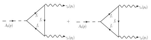
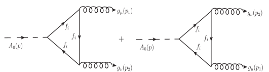
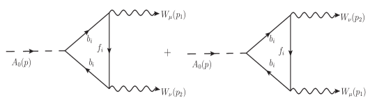
Figure 3: Feynman diagrams corresponding to the two-body decays of the pseudoscalar $A_{0}$ at one-loop level where $f_{i}\equiv b,t,T,T_{5}$, $T_{6}$, $T^{2/3}$, and $b_{i}\equiv b,B$.

We find that the generic decay widths of the $A_{0}\to\gamma\gamma,\gamma Z,ZZ,gg,WW$ processes at one-loop level are as follows:

$$\Gamma(A_{0}\to\gamma\gamma) = \frac{m^{3}_{A_{0}}}{256\pi^{5}}\bigg{|}\sum_{i}m_{f_{i}}\>g_{A_{0}f_{i}f_{i}}\,g^{2}_{\gamma f_{i}f_{i}}C_{0}(0,0,m_{A_{0}}^{2},m_{f_{i}}^{2},m_{f_{i}}^{2},m_{f_{i}}^{2})\bigg{|}^{2},$$ (8)

$$\Gamma(A_{0}\to\gamma Z) = \frac{m^{3}_{A_{0}}}{128\pi^{5}}\left(1-\frac{m^{2}_{Z}}{m^{2}_{A_{0}}}\right)^{3}\bigg{|}\sum_{i}m_{f_{i}}\>g_{A_{0}f_{i}f_{i}}\,g_{\gamma f_{i}f_{i}}\,g^{Zf_{i}f_{i}}_{V}$$ (9)

$$\times C_{0}(m_{A_{0}}^{2},m^{2}_{Z},0,m_{f_{i}}^{2},m_{f_{i}}^{2},m_{f_{i}}^{2})\bigg{|}^{2},$$

$$\Gamma(A_{0}\to ZZ) = \frac{1}{256\pi^{5}m_{A_{0}}}\left(1-\frac{4m^{2}_{Z}}{m^{2}_{A_{0}}}\right)^{-1/2}\bigg{|}\sum_{i}m_{f_{i}}\,g_{A_{0}f_{i}f_{i}}$$ (10)

$$\times \bigg{[}\left(m^{2}_{A_{0}}\left((g^{Zf_{i}f_{i}}_{A})^{2}-(g^{Zf_{i}f_{i}}_{V})^{2}\right)+4m^{2}_{Z}(g^{Zf_{i}f_{i}}_{V})^{2}\right)C_{0}(m^{2}_{A_{0}},m^{2}_{Z},m^{2}_{Z},m^{2}_{f_{i}},m^{2}_{f_{i}},m^{2}_{f_{i}})$$

$$+ 4(g^{Zf_{i}f_{i}}_{A})^{2}\left(B_{0}(m_{A_{0}}^{2},m_{f_{i}}^{2},m_{f_{i}}^{2})-B_{0}(m_{Z}^{2},m_{f_{i}}^{2},m_{f_{i}}^{2})\right)\bigg{]}\bigg{|}^{2},$$

$$\Gamma(A_{0}\to gg) = \frac{g_{s}^{4}m^{3}_{A_{0}}}{128\pi^{5}}\bigg{|}\sum_{i}m_{f_{i}}\,g_{A_{0}f_{i}f_{i}}C_{0}(0,0,m^{2}_{A_{0}},m^{2}_{f_{i}},m^{2}_{f_{i}},m^{2}_{f_{i}})\bigg{|}^{2},$$ (11)

$$\Gamma(A_{0}\to WW) = \frac{g^{4}}{512\pi^{5}m_{A_{0}}}\left(1-\frac{4m^{2}_{W}}{m^{2}_{A_{0}}}\right)^{-1/2}$$ (12)

$$\times \bigg{|}\sum_{i,j}m_{f_{i}}\>g_{A_{0}f_{i}f_{i}}\bigg{(}\left(-m_{f_{i}}^{2}+m_{b_{j}}^{2}+m_{W}^{2}\right)C_{0}(m^{2}_{A_{0}},m^{2}_{W},m^{2}_{W},m^{2}_{f_{i}},m^{2}_{f_{i}},m^{2}_{b_{j}})$$

$$+ B_{0}(m^{2}_{A_{0}},m^{2}_{f_{i}},m^{2}_{f_{i}})-B_{0}(m^{2}_{W},m^{2}_{b_{j}},m^{2}_{f_{i}})\bigg{)}$$

$$+ \sum_{i,j}m_{b_{j}}\>g_{A_{0}b_{j}b_{j}}\bigg{(}\left(-m_{b_{j}}^{2}+m_{f_{i}}^{2}+m_{W}^{2}\right)C_{0}(m^{2}_{A_{0}},m^{2}_{W},m^{2}_{W},m^{2}_{b_{j}},m^{2}_{b_{j}},m^{2}_{f_{i}})$$

$$+ B_{0}(m^{2}_{A_{0}},m^{2}_{b_{j}},m^{2}_{b_{j}})-B_{0}(m^{2}_{W},m^{2}_{f_{i}},m^{2}_{b_{j}})\bigg{)}\bigg{|}^{2}.$$

In Eqs. (8)-(12), the scalar Passarino-Veltman functions are represented by $C_{0}(0,0,m_{A_{0}}^{2},m_{f_{i}}^{2},m_{f_{i}}^{2},m_{f_{i}}^{2})$, $C_{0}(m_{A_{0}}^{2},m^{2}_{Z},0,m_{f_{i}}^{2},m_{f_{i}}^{2},m_{f_{i}}^{2})$, $C_{0}(m^{2}_{A_{0}},m^{2}_{Z},m^{2}_{Z},m^{2}_{f_{i}},m^{2}_{f_{i}},m^{2}_{f_{i}})$, $C_{0}(m^{2}_{A_{0}},m^{2}_{W},m^{2}_{W},m^{2}_{f_{i}},m^{2}_{f_{i}},m^{2}_{b_{j}})$, $B_{0}(m_{A_{0}}^{2},m_{f_{i}}^{2},m_{f_{i}}^{2})$, $B_{0}(m_{Z}^{2},m_{f_{i}}^{2},m_{f_{i}}^{2})$, $B_{0}(m^{2}_{W},m^{2}_{b_{j}},m^{2}_{f_{i}})$, $B_{0}(m^{2}_{A_{0}},m^{2}_{b_{j}},m^{2}_{b_{j}})$, and $B_{0}(m^{2}_{W},m^{2}_{f_{i}},m^{2}_{b_{j}})$. On the other hand, the effective couplings ($g_{\gamma f_{i}f_{i}}$, $g_{A_{0}f_{i}f_{i}}$, $g_{A_{0}b_{j}b_{j}}$, $g^{Zf_{i}f_{i}}_{A}$, and $g^{Zf_{i}f_{i}}_{V}$) are explicitly provided in Appendix A.

III Numerical results

In this section, we present the results for the decay widths and branching ratios of the $A_{0}\to$ $bb$, $tt$, $\gamma tt$, $\gamma bb$, $Ztt$, $Zbb$, $Wtb$, $h_{0}tt$, $h_{0}bb$, $WW$, $gg$, $ZZ$, $\gamma\gamma$, $\gamma Z$ processes. We also present our numerical analysis for the production via gluon fusion of the pseudoscalar $A_{0}$ at current and future colliders within the BLHM framework.

The BLHM parameters involved in our calculation are $m_{A_{0}}$, $\tan\beta$, and $f$. In this way, to establish a benchmark scenario, the pseudoscalar production cross section was calculated by setting the pseudoscalar mass to $m_{A_{0}}=500$ GeV ATLAS:2024jja ; ATLAS:2022rws ; ATLAS:2020gxx ; CMS:2019ogx . Given the value of $m_{A_{0}}$, we can determine the allowed range of values for the parameter $\tan\beta$ (the ratio of the vacuum expectation values of the two Higgs doublets), which is defined by the following equation JHEP09-2010 ; Kalyniak:2013eva :

$$1< \beta<\sqrt{\frac{2+2\sqrt{\big{(}1-\frac{m^{2}_{h_{0}}}{m^{2}_{A_{0}}}\big{)}\big{(}1-\frac{m^{2}_{h_{0}}}{4\pi v^{2}}\big{)}}}{\frac{m^{2}_{h_{0}}}{m^{2}_{A_{0}}}\big{(}1+\frac{m^{2}_{A_{0}}-m^{2}_{h_{0}}}{4\pi v^{2}}\big{)}}-1}.$$ tan (13)

With respect to the energy scale $f$, this parameter characterizes the scale of new physics and plays a central role in the generation of the masses of the new heavy quarks. Constraints on $f$ arise both from theoretical considerations, such as avoiding excessive fine-tuning in the heavy quark sector, and from experimental bounds on the production of these quarks: $f\in[1000,2000]$ GeV JHEP09-2010 ; Kalyniak:2013eva ; Godfrey:2012tf ; Cruz-Albaro:2024vjk . An additional set of parameters involved in our analysis are the Yukawa couplings $y_{i}$ ($i=1,2,3$), which are assigned the values $y_{1}=0.61$, $y_{2}=0.84$, and $y_{3}=0.35$ Martinez-Martinez:2024lez ; Cruz-Albaro:2024vjk ; Cruz-Albaro:2023pah ; Cruz-Albaro:2022kty .

We first investigate how variations in the parameters $f$ or $\beta$ affect the decay width of the $A_{0}\to X$ ($X\equiv$ $tt$, $bb$, $\gamma tt$, $\gamma bb$, $Ztt$, $Zbb$, $Wtb$, $h_{0}tt$, $h_{0}bb$, $WW$, $gg$, $ZZ$, $\gamma\gamma$, $\gamma Z$) processes. In Fig. 4(a), we illustrate the behavior of the decay width $\Gamma(A_{0}\to X)$ as a function of the scale $f$, while keeping $\tan\beta$ fixed at 3.0. From this figure, we observe that the largest contributions to $\Gamma(A_{0}\to X)$ arise from the two-body and three-body tree-level pseudoscalar decays $\Gamma(A_{0}\to t\bar{t})$ and $\Gamma(A_{0}\to\gamma t\bar{t})$, which represent the dominant and subdominant contributions, respectively, throughout the entire energy interval of the $f$ scale analysis: $\Gamma(A_{0}\to t\bar{t})=[1.26,1.42]$ GeV and $\Gamma(A_{0}\to\gamma t\bar{t})=[1.39,1.56]\times 10^{-1}$ GeV. In contrast, the $A_{0}\to h_{0}b\bar{b}$ decay provides the smallest contribution, i.e., $\Gamma(A_{0}\to h_{0}b\bar{b})=[8.34,8.21]\times 10^{-9}$ GeV while $f\in[1000,2000]$ GeV. It is important to note that $A_{0}\to X$ decays arising at one-loop level generate numerical contributions of the order of $10^{-4}-10^{-7}$ GeV. On the other hand, Fig. 4(b) shows our analysis of the impact of the $\beta$ parameter on $\Gamma(A_{0}\to X)$, with the $f$ energy scale fixed at 1000 GeV. In this scenario, the curves that generate the largest contributions to the decay width $\Gamma(A_{0}\to X)$ are again given by the tree-level pseudoscalar decays $A_{0}\to t\bar{t}$ and $A_{0}\to\gamma t\bar{t}$: $\Gamma(A_{0}\to t\bar{t})=[6.70,3.39\times 10^{-1}]$ GeV and $\Gamma(A_{0}\to\gamma t\bar{t})=[7.36\times 10^{-1},3.72\times 10^{-2}]$ GeV when $\beta\in[\tan^{-1}(1),\tan^{-1}(6)]$ rad. Additionally, the $A_{0}\to h_{0}b\bar{b}$ decay provides the most suppressed contribution, $\Gamma(A_{0}\to h_{0}b\bar{b})=[7.57\times 10^{-8},2.03\times 10^{-9}]$ GeV. As for the $A_{0}$ pseudoscalar decays arising at one-loop level, in this context the processes generate contributions of the order of $10^{-3}$ to $10^{-7}$ GeV, these contributions are slightly larger compared to those obtained in the $\Gamma(A_{0}\to X)$ vs. $f$ analysis scenario. As can be seen clearly in Figs. 4(a) and 4(b), $\Gamma(A_{0}\to X)$ depends mainly on the parameter $\beta$. This effect is evident in the curves of $\Gamma(A_{0}\to X)$ vs. $\beta$, which show a pronounced decrease of about one order of magnitude for larger values of $\beta$. In contrast, $\Gamma(A_{0}\to X)$ shows little sensitivity to changes in $f$ scale values; the corresponding curves decrease slightly as $f$ increases.

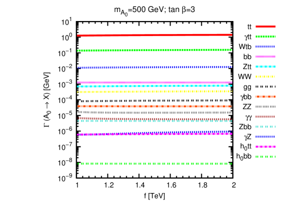
(a)

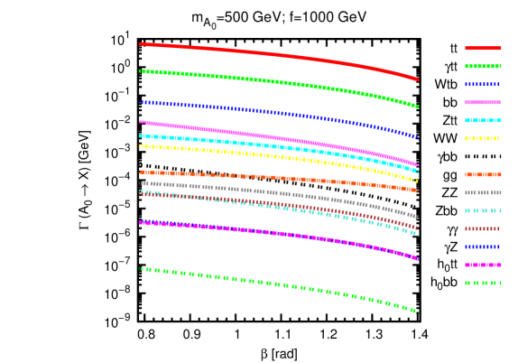
(b)

Figure 4: Decay widths for the $A_{0}\to X$ processes where $X\equiv$ $tt$, $bb$, $\gamma tt$, $\gamma bb$, $Ztt$, $Zbb$, $Wtb$, $h_{0}tt$, $h_{0}bb$, $WW$, $gg$, $ZZ$, $\gamma\gamma$, $\gamma Z$. a) $\Gamma(A_{0}\to X)$ as a function of the $f$ energy scale. b) $\Gamma(A_{0}\to X)$ as a function of the parameter $\beta$ ($\tan\beta\in[1,6]$).

Fig. 5 shows the corresponding branching ratios $\text{Br}(A_{0}\to X)$ for the $A_{0}\to X$ decays. The total decay width ($\Gamma_{A_{0}}$) of the pseudoscalar Higgs boson $A_{0}$ has been calculated taking into account the following pseudoscalar decay modes: $tt$, $bb$, $\gamma tt$, $\gamma bb$, $Ztt$, $Zbb$, $Wtb$, $h_{0}tt$, $h_{0}bb$, $WW$, $gg$, $ZZ$, $\gamma\gamma$, $\gamma Z$. In the left plot of Fig. 5, the dependence of $\text{Br}(A_{0}\to X)$ vs. $f$ is analyzed. In this plot, we see that the most probable decay channels of the pseudoscalar are given by the $A_{0}\to t\bar{t}$ and $A_{0}\to\gamma t\bar{t}$ processes when $f\in[1000,2000]$ GeV. These decays arise at tree level and generate dominant and subdominant contributions to $\text{Br}(A_{0}\to X)$: $\text{Br}(A_{0}\to t\bar{t})\approx 8.92\times 10^{-1}$ and $\text{Br}(A_{0}\to\gamma t\bar{t})\approx 9.81\times 10^{-2}$, respectively. While the numerical values do not show a strong sensitivity of $\text{Br}(A_{0}\to X)$ to $f$ at first glance, a variation becomes noticeable after a few digits beyond the decimal point. On the other hand, it is observed that the $A_{0}\to h_{0}b\bar{b}$ decay generates the smallest contribution to the branching ratio, that is, $\text{Br}(A_{0}\to h_{0}b\bar{b})=[5.90,5.17]\times 10^{-9}$. Regarding the right plot of Fig. 5, in this scenario we generate curves by varying the $\beta$ parameter while keeping the other parameter, $f$, fixed at 1000 GeV. In the corresponding figure, we see that the two main contributions are $\text{Br}(A_{0}\to t\bar{t})\approx 8.92\times 10^{-1}$ and $\text{Br}(A_{0}\to\gamma t\bar{t})=[9.80,9.81]\times 10^{-2}$ when $\beta\in[\tan^{-1}(1),\tan^{-1}(6)]$ rad. On the contrary, the most suppressed contribution is given by the $A_{0}\to h_{0}b\bar{b}$ decay which gives branching ratios of $\text{Br}(A_{0}\to h_{0}b\bar{b})=[1.01\times 10^{-8},5.35\times 10^{-9}]$ in the study interval for the $\beta$ parameter. Notably, in both study scenarios ($\text{Br}(A_{0}\to X)$ vs. $f$ and $\text{Br}(A_{0}\to X)$ vs. $\beta$), the one‑loop $A_{0}\to X$ decays produce branching ratios on the order of $10^{-4}$ to $10^{-7}$.

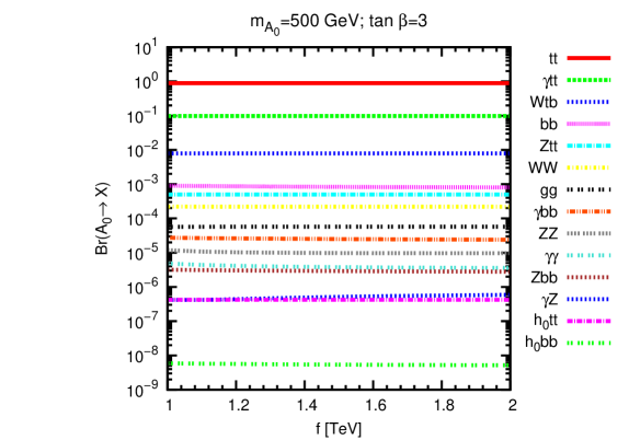
(a)

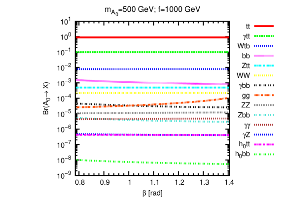
(b)

Figure 5: Branching ratios for the $A_{0}\to X$ processes where $X\equiv$ $tt$, $bb$, $\gamma tt$, $\gamma bb$, $Ztt$, $Zbb$, $Wtb$, $h_{0}tt$, $h_{0}bb$, $WW$, $gg$, $ZZ$, $\gamma\gamma$, $\gamma Z$. a) $\text{Br}(A_{0}\to X)$ as a function of the $f$ energy scale. b) $\text{Br}(A_{0}\to X)$ as a function of the parameter $\beta$ ($\tan\beta\in[1,6]$).

III.1 Production cross section of the pseudoscalar $A_{0}$ at the LHC and FCC-hh

In this subsection, we present the Breit-Wigner resonance formula, which is useful for describing the resonant production of the pseudoscalar Higgs boson $A_{0}$. Although Eq. (14) is determined just at the resonance of the pseudoscalar, it provides an approximate description of the pseudoscalar production mechanism via gluon fusion in the BLHM, it can also serve as a theoretical reference for guiding experimental searches for this new particle. Under this approximation, the production cross section of $A_{0}$ via gluon fusion can be expressed as follows pdg:2023 :

$$\sigma(gg\to A_{0}\to Y) = \frac{\pi}{36}\frac{\Gamma(A_{0}\to gg)\Gamma(A_{0}\to Y)}{m_{A_{0}}^{2}\Gamma^{2}_{A_{0}}},$$ (14)

where $\Gamma(A_{0}\to gg)$ and $\Gamma(A_{0}\to Y)$ (with $Y\equiv\gamma\gamma,\gamma Z,ZZ,gg,WW$) are the partial decay widths for an on-shell $A_{0}$ to decay to the initial and final states, respectively.

Using Eq. (14), we generated the curves shown in Fig. 6 for $m_{A_{0}}=500$ GeV, in which we studied the behavior of the cross section $\sigma(gg\to A_{0}\to Y)$ as a function of parameter $f$ or $\beta$, while fixing the other model parameters. We first discuss the behavior observed in Fig. 6(a) when $\tan\beta=3.0$. Note that the magnitude of $\sigma(gg\to A_{0}\to Y)$ depends slightly on the $f$ energy scale, except for the $gg\to A_{0}\to\gamma Z$ decay channel, which gives a curve with more appreciable changes within the range of study of the $f$ parameter, $f\in[1000,2000]$ GeV. In the same context, we find that the $gg\to A_{0}\to WW$ and $gg\to A_{0}\to\gamma Z$ decay channels generate the largest and smallest cross sections over the entire $f$ interval: $\sigma(gg\to A_{0}\to WW)=[1.70,1.71]\times 10^{-3}$ fb and $\sigma(gg\to A_{0}\to\gamma Z)=[3.21,4.57]\times 10^{-6}$ fb. Regarding Fig. 6(b), this plot shows the results for the pseudoscalar production cross section when the $f$ scale is fixed at $f=1000$ GeV, and the $\beta$ parameter varies within the range $\tan^{-1}(1)$ to $\tan^{-1}(6)$ rad. Once again, the $gg\to A_{0}\to WW$ process gives the largest contribution to $\sigma(gg\to A_{0}\to Y)$, while the $gg\to A_{0}\to\gamma Z$ decay channel yields the most suppressed contribution, i.e., $\sigma(gg\to A_{0}\to WW)=[7.68\times 10^{-4},3.26\times 10^{-3}]$ fb and $\sigma(gg\to A_{0}\to\gamma Z)=[1.68,6.06]\times 10^{-6}$ fb. The various curves obtained in the analysis of the $\sigma(gg\to A_{0}\to Y)$ production cross section as a function of $\beta$ exhibit a growth of up to two orders of magnitude as $\beta$ increases toward $1.4$ rad, as shown in the Fig. 6(b). It is evident that the region with the greater predictive importance corresponds to values of $\beta$ around 1.4 rad.

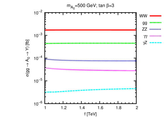
(a)

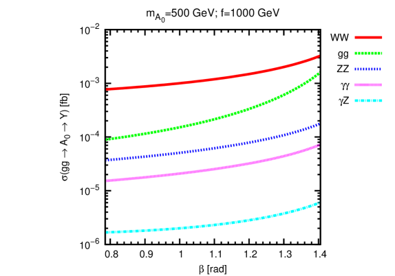
(b)

Figure 6: Production cross section of the pseudoscalar $A_{0}$ (for $m_{A_{0}}=500$ GeV) via gluon fusion. a) $\sigma(gg\to A_{0}\to Y)$ as a function of the $f$ energy scale. b) $\sigma(gg\to A_{0}\to Y)$ as a function of the parameter $\beta$ ($\tan\beta\in[1,6]$).

We now turn to discuss the dependence of $\sigma(gg\to A_{0}\to Y)$ on the $m_{A_{0}}$ parameter when it varies from 500 to 2000 GeV, as depicted in Fig. 7. In this figure, the curves have been generated for the values of $f=1000$ GeV and $\tan\beta=3$, as well as $f=2000$ GeV and $\tan\beta=6$. In the first scenario (see Fig. 7(a)), numerical evaluation shows that the $gg\to A_{0}\to WW$ decay channel provides the largest cross section when $m_{A_{0}}$ is approximately between 500 and 1360 GeV, $\sigma(gg\to A_{0}\to WW)=[5.10\times 10^{-3},3.69\times 10^{-5}]$ fb. Outside this range, the largest contribution comes from the $gg\to A_{0}\to ZZ$ process with $\sigma(gg\to A_{0}\to ZZ)=[3.69\times 10^{-5},9.17\times 10^{-6}]$ fb when $m_{A_{0}}\in[1360,2000]$ GeV. With respect to the second scenario (see Fig. 7(b)), again the $gg\to A_{0}\to WW$ and $gg\to A_{0}\to ZZ$ decay channels generate the largest contributions to $\sigma(gg\to A_{0}\to Y)$, i.e., $\sigma(gg\to A_{0}\to WW)=[3.30\times 10^{-3},1.94\times 10^{-5}]$ fb and $\sigma(gg\to A_{0}\to ZZ)=[1.94\times 10^{-5},3.93\times 10^{-6}]$ fb when $m_{A_{0}}\in[500,1160]$ GeV and $m_{A_{0}}\in[1160,2000]$ GeV, respectively. In both study scenarios, we observe that the pseudoscalar production cross section decreases as the mass of $A_{0}$ increases. It is also evident that $\sigma(gg\to A_{0}\to Y)$ strongly depends on the $m_{A_{0}}$ parameter. In general, the $gg\to A_{0}\to\gamma Z$ decay channel provides the smallest numerical contributions to $\sigma(gg\to A_{0}\to Y)$.

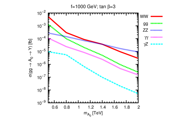
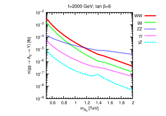
Figure 7: Production cross section of the pseudoscalar $A_{0}$ via gluon fusion as a function of the parameter $m_{A_{0}}$: a) $f=1000$ GeV and $\tan\beta=3$, and b) $f=2000$ GeV and $\tan\beta=6$.

In the experimental context, the production mechanism of the pseudoscalar $A_{0}$ via gluon fusion could be studied at the LHC, particularly in its future upgrades such as the High-Luminosity LHC (HL-LHC) and the High-Energy LHC (HE-LHC), as well as in future high-energy colliders like the FCC-hh. The HL-LHC ZurbanoFernandez:2020cco ; Azzi:2019yne ; Cepeda:2019klc ; FCC:2018bvk is planned to operate at a center-of-mass energy of 14 TeV with an integrated luminosity of 3000 fb^-1, while the HE-LHC ZurbanoFernandez:2020cco ; Azzi:2019yne ; Cepeda:2019klc ; FCC:2018bvk would provide proton-proton collisions at a center-of-mass energy of 27 TeV with an integrated luminosity of 10000 fb^-1. Accurate exploration of rare processes will be made possible by the LHC upgrades, which promise to increase the collision energy. As for the future hadron collider, the FCC-hh is designed to operate at a center-of-mass energy of $\sqrt{s}=100$ TeV and to collect a total integrated luminosity of 30000 fb^-1 MammenAbraham:2024gun ; Mangano:2022ukr ; FCC:2018byv ; FCC:2018vvp . This would allow the exploration of regions of parameter space that are currently inaccessible and would significantly increase the potential to study processes with extremely small cross sections. The FCC-hh is considered one of the most promising projects for the discovery of new particles in the coming decades.

Using the numerical results for the pseudoscalar production cross sections and considering the expected integrated luminosities of the HL-LHC, HE-LHC, and FCC-hh colliders, we can estimate the number of events that could be observed at these colliders for the $A_{0}\to Y$ pseudoscalar decays. Tables 1-5 present the expected number of events associated with the $A_{0}\to Y$ decays when the new physics scale $f$ takes specific values such as 1000 and 2000 GeV. It is important to emphasize that these event estimates have been generated by setting $m_{A_{0}}=500$ GeV. In this context, we find that the production of the pseudoscalar $A_{0}$ through the $A_{0}\to WW$ and $A_{0}\to gg$ decays (see Tables 1 and 2), which arise at one-loop level, provides very promising scenarios for the experiments of interest.

Table 1: The number of expected events related to $A_{0}\to WW$ decay.

	$m_{A_{0}}=500$ GeV, $\tan\beta=6$
$f$ [TeV]	No. of expected events at the colliders:
	HL-LHC	HE-LHC	FCC-hh
	$\mathcal{L}=3\,000$ fb-1	$\mathcal{L}=10\,000$ fb-1	$\mathcal{L}=30\,000$ fb-1
1	10	32	98
2	10	33	99

Table 2: The number of expected events related to $A_{0}\to gg$ decay.

	$m_{A_{0}}=500$ GeV, $\tan\beta=6$
$f$ [TeV]	No. of expected events at the colliders:
	HL-LHC	HE-LHC	FCC-hh
	$\mathcal{L}=3\,000$ fb-1	$\mathcal{L}=10\,000$ fb-1	$\mathcal{L}=30\,000$ fb-1
1	5	16	48
2	5	17	50

Table 3: The number of expected events related to $A_{0}\to ZZ$ decay.

	$m_{A_{0}}=500$ GeV, $\tan\beta=6$
$f$ [TeV]	No. of expected events at the colliders:
	HL-LHC	HE-LHC	FCC-hh
	$\mathcal{L}=3\,000$ fb-1	$\mathcal{L}=10\,000$ fb-1	$\mathcal{L}=30\,000$ fb-1
1	1	2	5
2	0	1	4

Table 4: The number of expected events related to $A_{0}\to\gamma\gamma$ decay.

	$m_{A_{0}}=500$ GeV, $\tan\beta=6$
$f$ [TeV]	No. of expected events at the colliders:
	HL-LHC	HE-LHC	FCC-hh
	$\mathcal{L}=3\,000$ fb-1	$\mathcal{L}=10\,000$ fb-1	$\mathcal{L}=30\,000$ fb-1
1	0	1	2
2	0	0	2

Table 5: The number of expected events related to $A_{0}\to\gamma Z$ decay.

	$m_{A_{0}}=500$ GeV, $\tan\beta=6$
$f$ [TeV]	No. of expected events at the colliders:
	HL-LHC	HE-LHC	FCC-hh
	$\mathcal{L}=3\,000$ fb-1	$\mathcal{L}=10\,000$ fb-1	$\mathcal{L}=30\,000$ fb-1
1	0	0	0
2	0	0	0

Additionally, Table 6 presents the number of events for the production of the pseudoscalar $A_{0}$ through the $A_{0}\to Y$ decays when $m_{A_{0}}=1000$ GeV is selected. It is important to mention that, for this benchmark scenario, only the FCC-hh appears to be within reach for the potential discovery of this new particle. The production of the pseudoscalar $A_{0}$ via gluon fusion would only be possible through the $A_{0}\to WW$, $A_{0}\to gg$, and $A_{0}\to ZZ$ decays.

Table 6: The number of expected events at the FCC-hh for the $A_{0}\to Y$ decay.

	$m_{A_{0}}=1000$ GeV, $\tan\beta=6$
$f$ [TeV]	No. of expected events at the FCC-hh:
	$A_{0}\to WW$	$A_{0}\to gg$	$A_{0}\to ZZ$	$A_{0}\to\gamma\gamma$	$A_{0}\to\gamma Z$
	$\mathcal{L}=30000$ fb-1	$\mathcal{L}=30000$ fb-1	$\mathcal{L}=30000$ fb-1	$\mathcal{L}=30000$ fb-1	$\mathcal{L}=30000$ fb-1
1	1	1	1	0	0
2	1	0	0	0	0

IV Conclusions

Within the BLHM framework, we investigate the production of the pseudoscalar $A_{0}$ through gluon fusion at future colliders, such as the HL-LHC, HE-LHC, and FCC-hh. These experiments promise to extend current searches for heavy particles, such as the pseudoscalar of interest to us.

In our study of the pseudoscalar $A_{0}$, we analyze the impact of the free parameters of the BLHM ($f$, $\beta$, and $m_{A_{0}}$) on the partial decay widths and branching fractions of the pseudoscalar, considering both two-and three-body decays at tree level, as well as one-loop level decays. For the one-loop decays, we account for the virtual particle effects induced by both the BLHM and SM particles. We also investigate the resonant production of the pseudoscalar $A_{0}$ using the Breit–Wigner resonance formula, evaluated specifically at the resonance peak of the pseudoscalar. Within this approach, we examine the sensitivity of the $\sigma(gg\to A_{0}\to Y)$ production cross section to the parameters $f$, $\beta$, and $m_{A_{0}}$, considering the following study intervals: $f\in[1000,2000]$ GeV, $\beta\in[\tan^{-1}(1),\tan^{-1}(6)]$ radians, and $m_{A_{0}}\in[500,2000]$ GeV. Our numerical results show that $\sigma(gg\to A_{0}\to Y)$ increases by up to two orders of magnitude as $\beta$ approaches 1.4 radians, indicating a strong dependence on this parameter. We find that the region of highest predictive significance corresponds to values of $\beta$ around approximately 1.4 radians. Additionally, we observe that the pseudoscalar production cross section decreases as the mass $m_{A_{0}}$ increases.

To establish a benchmark, Tables 1-5 present the expected number of events from the production of the pseudoscalar for two different mass values: $m_{A_{0}}=500$ GeV and $m_{A_{0}}=1000$ GeV. To estimate the number of events that could be observed at the colliders for the pseudoscalar decays $A_{0}\to Y$, we have considered the expected integrated luminosities of the HL-LHC, HE-LHC, and FCC-hh. In the first scenario, when $m_{A_{0}}=500$ GeV, we find that the production of the pseudoscalar $A_{0}$ through the $A_{0}\to WW$ and $A_{0}\to gg$ decay channels (see Tables 1 and  2), which arise at one-loop level, provide very promising scenarios for the experiments of interest. In the second scenario, when $m_{A_{0}}=1000$ GeV, only the FCC-hh appears to be within reach for the potential discovery of the pseudoscalar Higgs boson $A_{0}$. Furthermore, the study of the pseudoscalar $A_{0}$ at resonance is an excellent starting point for the search for new physics. Our study complements other studies in the context of present and future hadron-hadron, hadron-lepton, and lepton-lepton colliders on the production and decay of the pseudoscalar $A_{0}$.

Acknowledgements

E. Cruz-Albaro appreciates the postdoctoral stay at the Universidad Autónoma de Zacatecas, México. A.G.R. and M.A.H.R. thank SNII and PROFEXCE (México).

Declarations

Data Availability Statement: All data generated or analyzed during this study are included in this article.

Appendix A Effective couplings in the BLHM

In this Appendix, we present the effective couplings involved in our calculation of the production of the pseudoscalar $A_{0}$.

Table 7: Effective couplings involved in our calculation of the decay of the pseudoscalar boson $A_{0}$.

	Effective couplings
$g_{A_{0}\,t\bar{t}}$	$\frac{3c_{\beta}y_{1}y_{2}y_{3}}{\sqrt{y_{1}^{2}+y_{2}^{2}}\sqrt{y_{1}^{2}+y_{3}^{2}}}-\frac{2c_{\beta}s_{\beta}vy_{2}y_{3}(y_{3}^{2}-2y_{1}^{2})}{f\sqrt{y_{1}^{2}+y_{2}^{2}}(y_{1}^{2}+y_{3}^{2})}-\frac{3c_{\beta}s_{\beta}^{2}v^{2}y_{1}y_{2}y_{3}^{3}}{2f^{2}(y_{1}^{2}+y_{2}^{2})^{5/2}(y_{1}^{2}+y_{3}^{2})^{5/2}}\bigg{(}4y_{1}^{6}+4(2y_{2}^{2}+y_{3}^{2})y_{1}^{4}+y_{1}^{2}(4y_{2}^{4}+8y_{3}^{2}y_{2}^{2}-2\sqrt{y_{1}^{2}+y_{3}^{2}})+y_{2}^{2}(4y_{2}^{2}y_{3}^{2}+\sqrt{y_{1}^{2}+y_{3}^{2}})\bigg{)}$
$g_{A_{0}\,b\bar{b}}$	$-c_{\beta}y_{b}$
$g_{A_{0}\,T\bar{T}}$	$-\frac{c_{\beta}s_{\beta}vy_{1}^{2}}{f(y_{1}^{2}+y_{2}^{2})^{3/2}(y_{1}^{2}+y_{3}^{2})(y_{2}^{2}-y_{3}^{2})}\bigg{(}y_{1}^{4}(y_{2}^{2}+2y_{3}^{2})+y_{1}^{2}(8y_{2}^{2}y_{3}^{2}-2y_{3}^{4})-y_{2}^{2}(y_{2}^{4}+3y_{2}^{2}y_{3}^{2}-7y_{3}^{4})\bigg{)}$
$g_{A_{0}\,T_{5}\bar{T_{5}}}$	$-\frac{9c_{\beta}s_{\beta}vy_{1}^{2}y_{2}^{2}y_{3}^{2}}{f\left(y_{1}^{2}+y_{3}^{2}\right)^{\frac{3}{2}}\left(y_{3}^{2}-y_{2}^{2}\right)}$
$g_{A_{0}\,T_{6}\bar{T}_{6}}$	$\frac{c_{\beta}s_{\beta}vy_{1}}{f}$
$g_{A_{0}\,T^{23}\bar{T}^{23}}$	$\frac{c_{\beta}s_{\beta}vy_{1}\left(3y_{1}^{2}-5y_{3}^{2}\right)}{f\left(y_{1}^{2}+y_{3}^{2}\right)}$
$g_{A_{0}A_{0}h_{0}}$	$-\frac{1}{2}v\lambda_{0}sin(\alpha-\beta)sin(2\beta)$

Table 8: Vector and axial-vector coupling constants of the interaction vertex involving a gauge boson with a pair of fermions.

Vertex	Vector couplings	Axial-vector couplings
$\gamma t\bar{t}$	$g_{\gamma t\bar{t}}^{V}=\frac{2gs_{W}}{3}$	$g_{\gamma t\bar{t}}^{A}=0$
$\gamma b\bar{b}$	$g_{\gamma b\bar{b}}^{V}=-\frac{gs_{W}}{3}$	$g_{\gamma b\bar{b}}^{A}=0$
$\gamma T\bar{T}$	$g_{\gamma T\bar{T}}^{V}=\frac{2gs_{W}}{3}$	$g_{\gamma T\bar{T}}^{A}=\frac{gs_{W}v^{2}}{3f^{2}}\bigg{(}c_{\beta}^{2}-\frac{y_{1}^{2}(4c_{\beta}^{2}(y_{2}^{2}-y_{3}^{2})^{2}+s_{\beta}^{2}(2y_{2}^{2}+y_{3}^{2})^{2})}{(y_{1}^{2}+y_{2}^{2})(y_{2}^{2}-y_{3}^{2})^{2}}\hfill\break+\frac{s_{\beta}^{2}y_{3}^{2}(y_{2}^{2}-2y_{1}^{2})^{2}}{(y_{1}^{2}+y_{2}^{2})^{2}(y_{1}^{2}+y_{3}^{2})}\bigg{)}$
$\gamma T_{5}\bar{T_{5}}$	$g_{\gamma T_{5}\bar{T_{5}}}^{V}=\frac{2}{3}gs_{W}$	$g_{\gamma T_{5}\bar{T_{5}}}^{A}=\frac{3gs_{\beta}^{2}s_{W}v^{2}y_{1}^{2}y_{2}^{2}\left(y_{3}^{2}-y_{1}^{2}\right)}{2f^{2}\left(y_{1}^{2}+y_{3}^{2}\right)^{2}\left(y_{2}^{2}-y_{3}^{2}\right)}$
$\gamma T_{6}\bar{T_{6}}$	$g_{\gamma T_{6}\bar{T_{6}}}^{V}=\frac{2}{3}gs_{W}$	$g_{\gamma T_{6}\bar{T_{6}}}^{A}=-\frac{3c_{\beta}^{2}gs_{W}v^{2}}{4f^{2}}$
$\gamma T^{2/3}\bar{T}^{2/3}$	$g_{\gamma T^{2/3}\bar{T}^{2/3}}^{V}=\frac{2}{3}gs_{W}$	$g_{\gamma T^{2/3}\bar{T}^{2/3}}^{A}=\frac{gs_{\beta}^{2}s_{W}v^{2}}{f^{2}}$

Table 9: Continuation of Table 8.

Vertex	Vector couplings	Axial-vector couplings
$Zt\bar{t}$	$g_{Zt\bar{t}}^{V}=\frac{g}{c_{W}}(\frac{1}{4}-\frac{2s_{W}^{2}}{3})$	$g_{Zt\bar{t}}^{A}=\frac{g}{4c_{W}}$
$Zb\bar{b}$	$g_{Zb\bar{b}}^{V}=\frac{g}{c_{W}}(-\frac{1}{4}+\frac{s_{W}^{2}}{3})$	$g_{Zb\bar{b}}^{A}=-\frac{g}{4c_{W}}$
$ZT\bar{T}$	$g_{ZT\bar{T}}^{V}=\frac{g}{6c_{W}}\bigg{(}(3c_{W}^{2}-s_{W}^{2})\hfil\break-\frac{4s_{W}^{2}v^{2}y_{1}^{2}(4c_{\beta}^{2}(y_{2}^{2}-y_{3}^{2})^{2}+s_{\beta}^{2}(2y_{2}^{2}+y_{2})^{2})}{f^{2}(y_{1}^{2}+y_{2}^{2})(y_{2}^{2}-y_{3}^{2})^{2}}\bigg{)}$	$g_{ZT\bar{T}}^{A}=0$
$ZT_{5}\bar{T_{5}}$	$g_{ZT_{5}\bar{T_{5}}}^{V}=-\frac{2gs_{W}^{2}}{3c_{W}}$	$g_{ZT_{5}\bar{T_{5}}}^{A}=\frac{3gs_{\beta}^{2}v^{2}y_{1}^{2}y_{2}^{2}}{4c_{W}f^{2}(y_{1}^{2}+y_{3}^{2})^{2}(y_{2}^{2}-y_{3}^{2})^{2}}\bigg{(}(s_{W}^{2}y_{3}^{4}-c_{W}^{2}(y_{1}^{2}(y_{2}^{2}+2y_{3}^{2})-2y_{2}^{2}y_{3}^{2}+5y_{3}^{4}))-c_{W}^{2}(y_{1}^{2}+y_{3}^{2})(y_{2}^{2}-4y_{3}^{2})\bigg{)}$
$ZT_{6}\bar{T_{6}}$	$g_{ZT_{6}\bar{T_{6}}}^{V}=-\frac{g\left(8f^{2}s_{W}^{2}-15c_{\beta}^{2}c_{W}^{2}v^{2}\right)}{12c_{W}f^{2}}$	$g_{ZT_{6}\bar{T_{6}}}^{A}=-\frac{3gc_{W}c_{\beta}^{2}gv^{2}}{4f^{2}}$
$ZT^{2/3}\bar{T}^{2/3}$	$g_{ZT_{2/3}\bar{T}_{2/3}}^{V}=-\bigg{(}\frac{5gs_{\beta}^{2}s_{W}^{2}v^{2}}{3c_{W}f^{2}}+\frac{c_{W}g}{2}+\frac{7gs_{W}^{2}}{6c_{W}}\bigg{)}$	$g_{ZT_{2/3}\bar{T}_{2/3}}^{A}=-\frac{gs_{\beta}^{2}s_{W}^{2}v^{2}}{c_{W}f^{2}}$
$W^{+}\bar{t}b$	$g_{W\bar{t}b}^{V}=\frac{g}{2\sqrt{2}}$	$g_{W\bar{t}b}^{A}=-\frac{g}{2\sqrt{2}}$
$W^{+}\bar{T}_{5}b$	$g_{W\bar{T}_{5}b}^{V}=-\frac{gs_{\beta}vy_{2}(2y_{1}^{2}-y_{3}^{2})}{2\sqrt{2}f\sqrt{y_{1}^{2}+y_{2}^{2}}(y_{1}^{2}+y_{3}^{2})}$	$g_{W\bar{T}_{5}b}^{A}=\frac{gs_{\beta}vy_{2}(2y_{1}^{2}-y_{3}^{2})}{2\sqrt{2}f\sqrt{y_{1}^{2}+y_{2}^{2}}(y_{1}^{2}+y_{3}^{2})}$
$W^{+}\bar{T}_{6}b$	$g_{W\bar{T}_{6}b}^{V}=-\frac{\sqrt{2}c_{\beta}vy_{2}}{2f\sqrt{y_{1}^{2}+y_{2}^{2}}}$	$g_{W\bar{T}_{5}b}^{A}=\frac{\sqrt{2}c_{\beta}vy_{2}}{2f\sqrt{y_{1}^{2}+y_{2}^{2}}}$
$W^{+}\bar{T}B$	$g_{W\bar{T}B}^{V}=\frac{g}{2\sqrt{2}}$	$g_{W\bar{T}B}^{A}=-\frac{g}{2\sqrt{2}}$
$W^{+}\bar{T}_{5}B$	$g_{W\bar{T}_{5}B}^{V}=-\frac{gs_{\beta}vy_{1}(2y_{2}^{2}+y_{3}^{2})}{2\sqrt{2}f\sqrt{y_{1}^{2}+y_{2}^{2}}(y_{2}^{2}-y_{3}^{2})}$	$g_{W\bar{T}_{5}B}^{A}=\frac{gs_{\beta}vy_{1}(2y_{2}^{2}+y_{3}^{2})}{2\sqrt{2}f\sqrt{y_{1}^{2}+y_{2}^{2}}(y_{2}^{2}-y_{3}^{2})}$
$W^{+}\bar{T}_{6}B$	$g_{W\bar{T}_{6}B}^{V}=-\frac{\sqrt{2}c_{\beta}vy_{1}}{2f\sqrt{y_{1}^{2}+y_{2}^{2}}}$	$g_{W\bar{T}_{5}B}^{A}=\frac{\sqrt{2}c_{\beta}vy_{1}}{2f\sqrt{y_{1}^{2}+y_{2}^{2}}}$

References

- (1) G. Aad et al. (ATLAS Collaboration), Phys. Lett. B 716, 1 (2012).
- (2) S. Chatrchyan et al. (CMS Collaboration), Phys. Lett. B 716, 30 (2012).
- (3) A. Hayrapetyan et al. (CMS Collaboration), Phys. Lett. B 847, 138290 (2023).
- (4) G. Aad et al. (ATLAS Collaboration), Eur. Phys. J. C 83, 496 (2023); Erratum: Eur. Phys. J. C 84, 156 (2024).
- (5) C. Englert, A. Freitas, M. M. Mühlleitner, T. Plehn, M. Rauch, M. Spira and K. Walz, J. Phys. G 41, 113001 (2014).
- (6) M. Schmaltz, Nucl. Phys. B Proc. Suppl. 117, 40 (2003).
- (7) N. Arkani-Hamed, A. G. Cohen, E. Katz and A. E. Nelson, JHEP 07, 034 (2002).
- (8) S. Chang, JHEP 12, 057 (2003).
- (9) T. Han, H. E. Logan, B. McElrath and L. T. Wang, Phys. Rev. D 67, 095004 (2003).
- (10) S. Chang and J. G. Wacker, Phys. Rev. D 69, 035002 (2004).
- (11) M. Schmaltz, JHEP 08, 056 (2004).
- (12) M. Schmaltz and J. Thaler, JHEP 03, 137 (2009).
- (13) M. Schmaltz, D. Stolarski and J. Thaler, JHEP 09, 018 (2010).
- (14) S. Godfrey, T. Gregoire, P. Kalyniak, T. A. W. Martin and K. Moats, JHEP 04, 032 (2012).
- (15) P. Kalyniak, T. Martin and K. Moats, Phys. Rev. D 91, 013010 (2015).
- (16) J. M. Martínez-Martínez, A. Gutiérrez-Rodríguez, E. Cruz-Albaro and M. A. Hernández-Ruíz, Chin. Phys. C 49, 073101 (2025).
- (17) E. Cruz-Albaro, A. Gutiérrez-Rodríguez, D. Espinosa-Gómez, T. Cisneros-Pérez and F. Ramírez-Zavaleta, Phys. Rev. D 110, 015013 (2024).
- (18) E. Cruz-Albaro, A. Gutiérrez-Rodríguez, J. I. Aranda and F. Ramírez-Zavaleta, Eur. Phys. J. C 82, 1095 (2022).
- (19) I. Zurbano Fernandez, M. Zobov, A. Zlobin, F. Zimmermann, M. Zerlauth, C. Zanoni, C. Zannini, O. Zagorodnova, I. Zacharov and M. Yu, et al., High-Luminosity Large Hadron Collider (HL-LHC): Technical design report, CERN, 2020, ISBN 978-92-9083-586-8, 978-92-9083-587-5.
- (20) P. Azzi, S. Farry, P. Nason, A. Tricoli, D. Zeppenfeld, R. Abdul Khalek, J. Alimena, N. Andari, L. Aperio Bella and A. J. Armbruster, et al., CERN Yellow Rep. Monogr. 7, 1 (2019).
- (21) M. Cepeda, S. Gori, P. Ilten, M. Kado, F. Riva, R. Abdul Khalek, A. Aboubrahim, J. Alimena, S. Alioli and A. Alves, et al., CERN Yellow Rep. Monogr. 7, 221 (2019).
- (22) A. Abada et al. (FCC Collaboration), Eur. Phys. J. ST 228, 1109 (2019).
- (23) R. Mammen Abraham, J. Adhikary, J. L. Feng, M. Fieg, F. Kling, J. Li, J. Pei, T. R. Rabemananjara, J. Rojo and S. Trojanowski, JHEP 01, 094 (2025).
- (24) M. L. Mangano, W. Riegler, M. Aleksa, P. P. Allport, S. Asai, A. Ball, M. I. Besana, E. R. Bielert, S. Bologna and E. Boos, et al., Conceptual design of an experiment at the FCC-hh, a future 100 TeV hadron collider, doi:10.23731/CYRM-2022-002.
- (25) A. Abada et al. (FCC Collaboration), Eur. Phys. J. C 79, 474 (2019).
- (26) A. Abada et al. (FCC Collaboration), Eur. Phys. J. ST 228, 755 (2019).
- (27) G. Aad et al. (ATLAS Collaboration), Phys. Rev. Lett. 108, 111803 (2012).
- (28) G. Aad et al. (ATLAS and CMS Collaborations), Phys. Rev. Lett. 114, 191803 (2015).
- (29) A. Arhrib, R. Benbrik, J. El Falaki, M. Sampaio and R. Santos, Phys. Rev. D 99, 035043 (2019).
- (30) F. Abu-Ajamieh, S. Modak, S. Mukherjee and S. K. Vempati, Pseudoscalar Higgs Production at Muon Colliders: The Role of One-Loop Effective Vertices, arXiv:2505.02092 [hep-ph].
- (31) J. I. Aranda, E. Cruz-Albaro, D. Espinosa-Gómez, J. Montaño, F. Ramírez-Zavaleta and E. S. Tututi, J. Phys. G 44, 105002 (2017).
- (32) A. S. Cornell, A. Deandrea, B. Fuks and L. Mason, Phys. Rev. D 102, 035030 (2020).
- (33) M. M. Almarashi, Universe 7, 392 (2021).
- (34) G. Aad et al. (ATLAS Collaboration), Eur. Phys. J. C 85, 573 (2025).
- (35) G. Aad et al. (ATLAS Collaboration), JHEP 07, 203 (2023).
- (36) M. Aaboud et al. (ATLAS Collaboration), Phys. Rev. Lett. 119, 191803 (2017).
- (37) C. Kao, G. Lovelace and L. H. Orr, Phys. Lett. B 567, 259 (2003).
- (38) E. Cruz-Albaro, A. Gutierrez-Rodrıguez, M. A. Hernandez-Ruız and T. Cisneros-Perez, Eur. Phys. J. Plus 138, 506 (2023).
- (39) E. Cruz-Albaro and A. Gutiérrez-Rodríguez, Eur. Phys. J. Plus 137, 1295 (2022).
- (40) A. Gutiérrez-Rodríguez, E. Cruz-Albaro, D. Espinosa-Gómez, T. Cisneros-Pérez and D. A. Pérez-Carlos, New physics search with the new gauge boson of the bestest little Higgs model at the muon collider, arXiv:2312.08560 [hep-ph].
- (41) R. L. Workman et al. (Particle Data Group), Prog. Theor. Exp. Phys. 2022, 083C01 (2022).
- (42) V. D. Barger and R. J. N. Phillips, Collider Physics, Addison-Wesley (1996); V. D. Barger and R. J. N. Phillips, Collider Physics, Addison-Wesley (1997).
- (43) E. Barradas, J. L. Diaz-Cruz, A. Gutierrez and A. Rosado, Phys. Rev. D 53, 1678 (1996).
- (44) A. Denner and S. Dittmaier, Nucl. Phys. B 734, 62 (2006).
- (45) H. H. Patel, Comput. Phys. Commun. 197, 276 (2015).
- (46) H. H. Patel, Comput. Phys. Commun. 218, 66 (2017).
- (47) G. Aad, et al. (ATLAS Collaboration), Eur. Phys. J. C81, 396 (2021).
- (48) A. M. Sirunyan et al. (CMS Collaboration), JHEP 03, 055 (2020).