Unbounded knapsack problem and double partitions

Abstract

The unbounded knapsack problem can be considered as a particular case of the double partition problem that asks for a number of nonnegative integer solutions to a system of two linear Diophantine equations with integer coefficients. In the middle of 19th century Sylvester and Cayley suggested an approach based on the variable elimination allowing a reduction of a double partition to a sum of scalar partitions. This manuscript discusses a geometric interpretation of this method and its application to the knapsack problem.

Keywords: unbounded knapsack problem, double partition.

2010 Mathematics Subject Classification: 11P82.

1 Integer partitions and knapsack problem

The intimate relation between the knapsack problem and integer partitions attracted attention of many researchers [1, 3, 4] who mainly focused on the algorithmic approaches while the partition computational aspect was usually neglected. It happened probable because in the field of partitions there existed no explicit expressions for both scalar and vector partitions (to the latter the knapsack problem can be reduced). The author of this manuscript provided a closed formula for evaluation of scalar partitions based on the Bernoulli polynomials of higher order [6]. In the middle of the 19th century Sylvester suggested an algorithm of reduction of the vector partition to the sum of scalar ones [10] and Cayley successfully implemented it for the case of double partitions [2]. This manuscript discusses the application of the original Cayley method to the unbounded knapsack problem and provides a simple geometric interpretation of the algorithm.

1.1 Scalar partitions

The problem of integer partition into a set of integers is equivalent to a problem of number of nonnegative integer solutions of the Diophantine equation

$$s=\sum_{i=1}^{m}x_{i}d_{i}={\bf x}\cdot{\bf d}.$$ (1)

A scalar partition function $W(s,{\bf d})\equiv W(s,\{d_{1},d_{2},\ldots,d_{m}\})$ solving the above problem is a number of partitions of an integer $s$ into positive integers $\{d_{1},d_{2},\ldots,d_{m}\}$. The generating function for $W(s,{\bf d})$ has a form

$$G(t,{\bf d})=\prod_{i=1}^{m}\frac{1}{1-t^{d_{i}}}=\sum_{s=0}^{\infty}W(s,{\bf d})\;t^{s}\;,$$ (2)

Sylvester proved [11] a statement about splitting of the scalar partition into periodic and non-periodic parts and showed that it may be presented as a sum of the so called Sylvester waves

$$W(s,{\bf d})=\sum_{n=1}W_{n}(s,{\bf d})\;,$$ (3)

where summation runs over all distinct factors of the elements of the generator vector ${\bf d}$. The wave $W_{n}(s,{\bf d})$ is a quasipolynomial in $s$ given by a product of a polynomial multiplied by a periodic function with period $n$. It was shown [6] that it is possible to express the wave $W_{n}(s,{\bf d})$ as a finite sum of the Bernoulli polynomials of higher order.

1.2 Vector partitions

Consider a function $W({\bf s},{\bf D})$ counting the number of integer nonnegative solutions ${\bf x}\geq 0$ to a linear system ${\bf s}={\bf D}\cdot{\bf x}$, where ${\bf s}=\{s_{1},s_{2},\ldots,s_{l}\}$ and ${\bf D}=\{{\bf c}_{1},{\bf c}_{2},\ldots,{\bf c}_{m}\}$ is a nonnegative integer $l\times m$ generator matrix made of $m$ columns ${\bf c}_{i}=\{c_{i1},c_{i2},\ldots,c_{il}\},\ (1\leq i\leq m\leq l)$ where some elements $c_{ik}$ might equal zero. The function $W({\bf s},{\bf D})$ called vector partition is a natural generalization of scalar partition to the vector argument. The generating function for $W({\bf s},{\bf D})$ reads

$$G({\bf t},{\bf D})=\prod_{i=1}^{m}\frac{1}{1-{\bf t}^{{\bf c}_{i}}}=\sum_{{\bf s}}W({\bf s},{\bf D}){\bf t^{s}},\quad{\bf t^{s}}=\prod_{k=1}^{l}t_{k}^{s_{k}},\quad{\bf t}^{{\bf c}_{i}}=\prod_{k=1}^{l}t_{k}^{c_{ik}}.$$ (4)

1.3 Sylvester-Cayley method of vector partition reduction

The problem of scalar and vector integer partitions has a long history and J.J. Sylvester made a significant contribution to its solution. In addition to the splitting algorithm for scalar partition [11] he suggested [10] to reduce vector partition into a sum of scalar partitions. The reduction is an iterative process based on elimination of the variable $t_{i}$ in the generating function (4) which is equivalent to the elimination of $x_{i}$ from the system ${\bf s}={\bf D}\cdot{\bf x}$. Sylvester considered a specific double partition problem as an illustration of his method and determined regions (chambers) each characterized by a unique expression for vector partition valid in this region only. He showed that the expressions in the adjacent chambers coincide at their common boundary.

This approach was successfully applied by A. Cayley [2] to double partitions subject to restrictions on the elements of the matrix ${\bf D}$ – the vectors ${\bf c}_{i}$ should be noncollinear and the elements of every column ${\bf c}_{i}$ must be relatively prime – which were first specified by Sylvester in his lectures [9]. The detailed description of the Cayley algorithm derivation is presented in [7, 8] where this method is generalized in order to perform the reduction to scalar partitions in the cases when the conditions imposed on the matrix ${\bf D}$ elements are not satisfied. In this manuscript we consider the application of the original Cayley algorithm to the unbounded knapsack problem.

1.4 Knapsack problem as double partition

The unbounded knapsack problem (UKP) reads [5]

$$\mbox{maximize}\quad V=\sum_{i=1}^{m}v_{i}x_{i},\quad\mbox{subject to}\quad\sum_{i=1}^{m}w_{i}x_{i}\leq W,$$ (5)

for nonnegative integer $x_{i}$. Introduce a slack variable $x_{0}$ with the corresponding values $w_{0}=1,v_{0}=0$ and rewrite the problem (5) as a system of the two Diophantine equations

$$\sum_{i=0}^{m}w_{i}x_{i}=W,\quad\quad\sum_{i=0}^{m}v_{i}x_{i}=V,$$ (6)

to find $M(W)=\mbox{max}\,V$ for the fixed value of $W$. We also assume that the nonnegative integers $w_{i},v_{i}$ satisfy the conditions relation

$$\gamma_{m}>\gamma_{m-1}>\ldots\gamma_{2}>\gamma_{1}>\gamma_{0}=0,\quad\gamma_{i}=v_{i}/w_{i},\quad\mbox{gcd}(v_{i},w_{i})=1,\quad 0\leq i\leq m,$$ (7)

where $\mbox{gcd}(v_{i},w_{i})$ denotes the greatest common divisor of $v_{i}$ and $w_{i}$. The system of the two Diophantine equations (6) corresponds to the problem ${\bf s}={\bf D}\cdot{\bf x}$ with ${\bf D}=\{{\bf c}_{0},{\bf c}_{1},{\bf c}_{2},\ldots{\bf c}_{m-1},{\bf c}_{m}\}$ and ${\bf s}=\{W,V\}^{T}$, where ${\bf c}_{0}=\{1,0\}^{T}$, ${\bf c}_{i}=\{w_{i},v_{i}\}^{T},\ (1\leq i\leq m),$ are the two-dimensional columns of the matrix ${\bf D}$ and ^T denotes the transposition.

The UKP can be stated as follows – for the fixed value of $W$ find the maximal value $M(W)$ of $V$ for which the double partition $W({\bf s},{\bf D})>0$. The condition $\mbox{gcd}(w_{i},v_{i})=1$ means that all columns ${\bf c}_{i}$ are prime ones while the inequalities in (7) guaranties that the matrix ${\bf D}$ has no collinear columns. These conditions coincide with those specified for application of the variable elimination algorithm. Thus the value of the double partition $W({\bf s},{\bf D})$ can be expressed as a sum of scalar partitions that in their turn can be computed through the Bernoulli polynomials of higher order. This means that the UKP solution can be found as a closed formula with the finite number of quasipolynomials terms.

2 Double partition reduction by variable elimination

The process of variable elimination in a system of linear equations is well known and is widely used in the high school algebra course where it is applied for the solution of a system of $m$ equations with $m$ unknowns. In this section we describe a generalization of the elimination method for a system of two Diophantine equations with $m+1$ variables $x_{i},\ 0\leq i\leq m$. Write the system (6) as follows

$${\bf s}=\sum_{i=0}^{m}{\bf c}_{i}x_{i},$$ (8)

and consider the elimination procedure of the variable $x_{j}$. Introduce the integer vector ${\bf n}_{j}$ normal to ${\bf c}_{j}$ satisfying the relations (see Fig.1)

$${\bf n}_{j}=\{v_{j},-w_{j}\},\quad{\bf n}_{j}\cdot{\bf c}_{j}=0,\quad{\bf n}_{j}\times{\bf c}_{j}=1,$$ (9)

where ${\bf a}\cdot{\bf b}$ and ${\bf a}\times{\bf b}$ denote the scalar and vector product of two vectors respectively. Multiply the vector equation (8) by ${\bf n}_{j}$ to obtain

$$l_{j}=\sum_{i=0}^{m}d_{ji}x_{i},\quad l_{j}={\bf s}\cdot{\bf n}_{j}=Wv_{j}-Vw_{j},\quad d_{ji}={\bf c}_{i}\cdot{\bf n}_{j}=w_{i}v_{j}-v_{i}w_{j},\quad d_{jj}\equiv 0.$$ (10)

The equation (10) gives rise to the scalar partition $W_{j}({\bf s})=W(l_{j},{\bf d}_{j})$ with the set ${\bf d}_{j}=\{d_{j0},d_{j1},d_{j2},\ldots,d_{jm}\}$ of $m$ positive integers $d_{ji},\ i\neq j$. The theorem proved by Cayley [2] states that the value of the double partition $W({\bf s},{\bf D})$ is given be the sum of $(m+1)$ scalar partitions

$$W({\bf s},{\bf D})=\sum_{j=0}^{m}W_{j}({\bf s})=\sum_{j=0}^{m}W(l_{j},{\bf d}_{j}).$$ (11)

The elements of the vector ${\bf d}_{j}$ as well as the integer $l_{j}$ might be either positive or negative while $l_{j}$ might also vanish. From the definition of the scalar partition it follows that $W(s,{\bf d})=0$ for the negative $s<0$ and $W(0,{\bf d})=1$. One has to find a way to evaluate the partition $W(l_{j},{\bf d}_{j})$ in case when several $d_{ji}$ are negative. Assume that $d_{ji}<0$ for $0\leq i\leq k<m$, write the generating function of the scalar partition (2)

$$G(t,{\bf d}_{j})=\prod_{i=0}^{m}\frac{1}{1-t^{d_{ji}}},\quad i\neq j,$$

and use the relation

$$\frac{1}{1-t^{-a}}=-\frac{t^{a}}{1-t^{a}},$$ (12)

to rewrite $G(t,{\bf d}_{j})$ as follows

$$G(t,{\bf d}_{j})=(-1)^{k+1}\prod_{i=0}^{k}t^{|d_{ji}|}\cdot\prod_{i=0}^{m}\frac{1}{1-t^{|d_{ji}|}},\quad i\neq j.$$ (13)

Using the definition (2) of scalar partition as the coefficent of the generating function expansion we obtain

$$W(l_{j},{\bf d}_{j})=(-1)^{k+1}W(l_{j}+\sum_{i=0}^{k}d_{ji},|{\bf d}_{j}|),\quad|{\bf d}_{j}|=\{|d_{ji}|\}.$$ (14)

3 Sum of scalar partitions for knapsack problem solution

To apply the result of the double partition reduction into the sum of scalar partitions we first have to analyze the individual terms in (11).

3.1 Scalar partition analysis and evaluation

Considering the element $d_{ji}={\bf c}_{i}\cdot{\bf n}_{j}$ we observe that this element is positive when the angle between the vectors ${\bf c}_{i}$ and ${\bf n}_{j}$ is less than $\pi/2$ and is negative when the angle exceeds $\pi/2$. Using the inequalities (7) we find that $d_{ji}>0$ for $j>i$ and $d_{ji}<0$ for $j<i$ (see Fig.1 for illustration and [9]). Similarly, the sign of $l_{j}$ is not fixed as it depends on the angle between ${\bf s}$ and ${\bf n}_{j}$ – if $\gamma_{j}>\Gamma=V/W$ we obtain $l_{j}>0$, when $\gamma_{j}<\Gamma$ the value of $l_{j}$ is negative and finally $l_{j}=0$ for $\gamma_{j}=\Gamma$. Using Fig.1 it is easy to observe that for any integer point ${\bf s}=\{w,v\}^{T}$ with $v/w>\gamma_{m}$ all summands $W_{j}({\bf s})$ equal zero and the double partition $W({\bf s},{\bf D})$ vanishes. This means that in order to find $M(W)$ one has to test only a finite number of points ${\bf s}=\{W,V\}^{T}$ with $0<V\leq v_{m}$, where $v_{j}=\lfloor W\gamma_{j}\rfloor$ and $\lfloor x\rfloor$ denotes integer part of $x$.

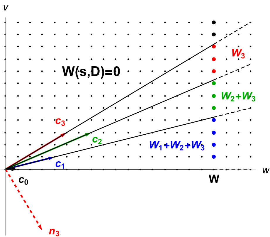
Figure 1: The arrows show the vectors ${\bf c}_{i}$ for the knapsack problem: ${\bf c}_{0}=\{1,0\}$ (black), ${\bf c}_{1}=\{4,1\}$ (blue), ${\bf c}_{2}=\{7,3\}$ (green), ${\bf c}_{3}=\{5,3\}$ (red); the normal ${\bf n}_{3}$ is shown by red dashed arrow. The double partition $W({\bf s},{\bf D})$ vanishes at all points that lie above the ray extending the vector ${\bf c}_{3}$. To determine $M(W)$ one has to evaluate $W({\bf s},{\bf D})$ only at the integer points ${\bf s}=\{W,V\}$ with $0<V\leq\lfloor W\gamma_{3}\rfloor$. The nonzero contributions of $W_{j}({\bf s})$ into $W({\bf s},{\bf D})$ are shown in the corresponding chambers. The value of $W({\bf s},{\bf D})$ at the red points is determined by $W_{3}({\bf s})$ only, while for the green and blue points one has to use the sum $W_{2}({\bf s})+W_{3}({\bf s})$ and $W_{1}({\bf s})+W_{2}({\bf s})+W_{3}({\bf s})$, respectively.

Applying this analysis we observe that the term $W_{m}({\bf s})$ has all $d_{mi}$ positive while $l_{m}>0$ for $0<V\leq v_{m}$. This means that the contribution of this term to the double partition is positive.

The term $W_{m-1}({\bf s})$ has a single negative element $d_{m-1,m}<0$ and $l_{m-1}>0$ for $0<V\leq v_{m-1}$ while $l_{m-1}<0$ for $v_{m-1}<V\leq v_{m}$ and in this range the single term $W_{m}({\bf s})$ contributes to the double partition. We find that the term $W_{m-1}({\bf s})$ contributes negatively

$$W_{m-1}({\bf s})=-W(l_{m-1}+d_{m-1,m},|{\bf d}_{m-1}|).$$

Similarly we find that the term $W_{m-2}({\bf s})$ generates positive contribution

$$W_{m-2}({\bf s})=W(l_{m-2}+d_{m-1,m}+d_{m-2,m-1},|{\bf d}_{m-2}|).$$

and it is nonzero for $0<V\leq v_{m-2}$, so that in the range $v_{m-2}<V\leq v_{m-1}$ the two terms $W_{m}({\bf s})$ and $W_{m-1}({\bf s})$ contribute to the double partition with opposite signs.

Continuing this process we find that the last term $W_{0}({\bf s})$ of the expansion (11) has $l_{0}<0$ and all $d_{0i}<0$ so that it does not contribute into the double partition. Thus the number of nonzero terms $W_{j}({\bf s})$ equals the number $m$ of the terms in the original problem (5) and the contribution of these terms is sign alternating.

3.2 Search algorithm for $M(W)$

The analysis done in the preceding Sections allows to split the interval $I=[1,v_{m}]$ inside which the search should be performed into $m$ subintervals $I_{j}=[v_{j-1}+1,v_{j}]$. The expression for the double partition $W({\bf s},{\bf D})$ inside the subinterval $I_{j}$ is given by the partial sum

$$W_{j}({\bf s},{\bf D})=\sum_{k=j}^{m}W_{k}({\bf s})=\sum_{k=j}^{m}(-1)^{m-k}W(l_{j}+\sum_{n=j}^{m-1}d_{n,n+1},|{\bf d}_{j}|),$$ (15)

with the alternating signs of the consecutive contributions.

As we are searching the maximal value $V$ for which $W({\bf s},{\bf D})\neq 0$ we scan the subintervals in the descending order of $V$. Note that inside the subinterval all the parameters in (15) are fixed except the value of $l_{j}=Wv_{j}-Vw_{j}$ that increases with the decreasing value of $V$.

We start from the top subinterval $I_{m}$ where $W_{m}({\bf s},{\bf D})$ is given by a single positive scalar partition $W_{m}({\bf s})$ scanning it starting with $V=v_{m}$. The first nonzero value of $W_{m}({\bf s})$ gives $M(W)$. If the search inside $I_{m}$ fails we move onto $I_{m-1}$ where $W_{m-1}({\bf s},{\bf D})$ is provided by the sum of two opposite sign terms. Thus for each $V$ we evaluate $W_{m}({\bf s})$ and if it is zero we move to the next value, otherwise we have to find the value of $W_{m-1}({\bf s})$ to check whether it cancels or not the first term in $W_{m-1}({\bf s},{\bf D})$. In the subinterval $I_{m-2}$ we first find the sum $W_{m}({\bf s})+W_{m-1}({\bf s})$ and only when it is zero we move on to compute $W_{m-2}({\bf s})$. The procedure repeated until the value $M(w)$ is determined.

References

- [1] G.H. Bradley, Transformation of Integer Programs to Knapsack Problems, Discr. Math. 1 (1971), 29-45.
- [2] A. Cayley, On a Problem of Double Partitions, Philosophical Magazine XX (1860), 337-341; Coll. Math. Papers, Cambridge Univ. Press, IV (1891), 166-170.
- [3] B. Faaland, Technical Note – Solution of the Value-Independent Knapsack Problem by Partitioning, Operations Research 21(1) (1973), 332-337.
- [4] E. Horowitz, S. Sahni, Computing Partitions with Appplications to the Knapsack Problem, J. Assoc. Comp. Mashinery 21 (1974), 277-292.
- [5] S. Martello, P. Toth, Knapsack problems: Algorithms and Computer Implementations, John Wiley amd Sons (1990), p.91.
- [6] B.Y. Rubinstein, Expression for Restricted Partition Function through Bernoulli Polynomials, Ramanujan Journal 15 (2008), 177-185.
- [7] B.Y. Rubinstein, On Cayley algorithm for double partition, arxiv (2023), arXiv:2310.00538v1 [math.CO].
- [8] B.Y. Rubinstein, On the Sylvester program and Cayley algorithm for vector partition reduction, arxiv (2025), arXiv:203.18789v3 [math.NT].
- [9] J.J.Sylvester, Outlines of Seven Lectures on the Partitions of Numbers, Proc. London Math. Soc. XXVIII (1897), 33–96; Coll. Math. Papers, Cambridge Univ. Press, II (1908), 119-175.
-
[10]
J.J. Sylvester, On the Problem of the Virgins, and the
General Theory of Compound Partitions,
Philosophical Magazine XVI (1858), 371-376; Coll. Math. Papers, Cambridge Univ. Press, II (1908), 113-117. - [11] J.J. Sylvester, On Subinvariants, i.e. Semi-invariants to Binary Quantics of an Unlimited Order. With an Excursus on Rational Fractions and Partitions, American J. of Math. 5 (1882), 79-136; Coll. Math. Papers, Cambridge Univ. Press, III (1909), 568-622.