Neural Inference of Fluid–Structure Interactions from
Sparse Off-Body Measurements

Abstract

We report a novel physics-informed neural framework for reconstructing unsteady fluid–structure interactions (FSI) from sparse, single-phase observations of the flow. Our approach combines modal surface models with coordinate neural representations of the fluid and solid dynamics, constrained by the fluid’s governing equations and an interface condition. Using only off-body Lagrangian particle tracks and a moving-wall boundary condition, the method infers both flow fields and structural motion. It does not require a constitutive model for the solid nor measurements of the surface position, although including these can improve performance. Reconstructions are demonstrated using two canonical FSI benchmarks: vortex-induced oscillations of a 2D flapping plate and pulse-wave propagation in a 3D flexible pipe. In both cases, the framework achieves accurate reconstructions of flow states and structure deformations despite data sparsity near the moving interface. A key result is that the reconstructions remain robust even as additional deformation modes are included beyond those needed to resolve the structure, eliminating the need for truncation-based regularization. This represents a novel application of physics-informed neural networks for learning coupled multiphase dynamics from single-phase observations. The method enables quantitative FSI analysis in experiments where flow measurements are sparse and structure measurements are asynchronous or altogether unavailable.

Keywords: fluid–structure interactions, physics-informed neural networks, Lagrangian particle tracking, flow reconstruction, inverse problems

1 Introduction

Fluid–structure interactions (FSI) arise when a flexible structure is immersed in or contains a flowing fluid. They appear in a wide range of applications, including flapping-wing aerodynamics [1, 2], offshore structures and wind turbines [3, 4], cardiovascular systems [5], and flow-induced vibrations [6]. Accurately resolving these interactions is essential for understanding the underlying physics and improving the performance of engineering devices. Traditional computational methods for FSI, such as the arbitrary Lagrangian–Eulerian (ALE) [7, 8], level set [9, 10], fictitious domain [11, 12], and immersed boundary [13, 14] methods, have enabled high-fidelity simulations by capturing moving boundaries and coupling fluid and solid domains. Each approach offers trade-offs in numerical stability, geometric flexibility, and computational cost. These methods work well for systems with well-defined boundary conditions and known material models [15, 16], but their application to real-world FSI often faces serious limitations. In particular, inflow/outflow boundary conditions and material properties may be unknown, and resolving small-scale dynamics at a complex interface can be prohibitively expensive.

In such cases, experimental measurements are essential, but the data are often sparse, noisy, and limited to a single phase (typically the fluid). This creates a disconnect: simulations provide the rich spatio-temporally resolved fields necessary for analyzing FSI dynamics, yet they are highly sensitive to uncertain boundary conditions and constitutive models. On the other hand, experiments indicate the actual system behavior but provide incomplete information. To leverage the strengths of both, we propose a data assimilation (DA) method that uses sparse, off-body measurements of the fluid to reconstruct both the flow field and the structural response, i.e., without requiring a constitutive model for the solid or direct measurements thereof. Our approach combines the fluid’s governing equations with partial observations to produce physically consistent reconstructions, even when conventional simulations are infeasible due to unknown boundary conditions or uncertain material models. This capability is especially valuable in FSI involving complex interfaces or biological materials, where structural properties are poorly characterized and simultaneous two-phase measurements are impractical or impossible.

There are two major strategies for simultaneously measuring the fluid and solid phases in FSI [17, 18]. The first combines two separate modalities, each with distinct illumination and/or detection wavelengths. For example, synchronous particle image velocimetry (PIV) and digital image correlation (DIC) have been used to study hydrodynamic loading and structural response [19], jet interactions with compliant surfaces [20], and supersonic panel flutter [21]. While these setups offer high-resolution, low-interference measurements of both phases, they are costly and require complex calibration. To reduce experimental overhead, a second strategy uses a single measurement modality, typically optimized for the fluid phase, and segments the fluid and solid in post-processing. For instance, PIV [22] and Lagrangian particle tracking (LPT) [23] have been used to capture both flow and surface motion by embedding particles on the structure. These surface particles can be distinguished from fluid tracers based on spatial location (e.g., lying on the outermost surface) or velocity (e.g., moving more slowly than the advected particles). However, such single-modality approaches face challenges, including optical interference, complex data processing, and inherently lower resolution, as fewer particles are available per phase due to tracking limits. The present work develops an inversion algorithm tailored to this second class of experiments (but applicable to both), using single-phase measurements to infer the flow and structure dynamics, a strategy that is extensible to other non-invasive modalities such as magnetic resonance velocimetry (MRV) [24].

Several algorithms have recently been developed to reconstruct FSI from single-phase data. For instance, Kontogiannis et al. [25] reported a Bayesian method for joint flow reconstruction and boundary segmentation from noisy MRV data. They modeled the 2D domain boundary using a signed distance function and employed an adjoint-based solver to optimize the inflow condition and boundary shape, subject to a hard constraint on the governing equations. Their approach yielded accurate reconstructions for steady 2D flows with fixed boundaries. Karnakov et al. [26] used optimizing a discrete loss (ODIL), a grid-based inverse solver that minimizes a composite loss function with soft constraints on the measurements and governing equations. ODIL minimizes the loss with a Newton solver and can recover flow and structure states from sparse velocity data, inheriting the convergence and stability properties of traditional solvers in some cases. For FSI problems, the ODIL loss penalizes residuals from the discretized Navier–Stokes equations and a no-slip boundary condition, with additional regularization applied to the level set representation of the surface. However, the method struggles with non-convex or geometrically complex shapes, tending to approximate them as simpler convex forms, and its computational cost grows rapidly with domain size and time in large-scale 3D or unsteady problems. More recently, Buhendwa et al. [27] extended ODIL by integrating it into the JAX-Fluids solver to infer 3D obstacle shapes and flow fields in steady supersonic flows. By using explicit shock-capturing schemes and level set representations of the boundary, they achieved accurate shape reconstructions even in shock-dominated regimes. While these methods provide a strong foundation for FSI reconstruction, dynamic problems involving complex geometries remain challenging due to limitations in computational efficiency, numerical stability, and the observability (or lack thereof) of unsteady boundary dynamics.

Physics-informed neural networks (PINNs) [28] are a machine learning technique with the potential to overcome key limitations of shape inference in DA for FSI. PINNs use one or more neural networks, often termed coordinate neural networks, to map space–time input coordinates to the corresponding flow or structure fields at those locations. Physical consistency is weakly enforced by incorporating residuals of the governing equations into the networks’ loss function. Numerous studies have demonstrated the effectiveness of PINNs for inverse problems in FSI. Raissi et al. [29] were among the first to establish the foundation for PINNs in this context, applying them to vortex-induced vibrations of a rigid cylinder elastically mounted in a uniform 2D flow. Using scattered data, including the concentration of an advected scalar and structural displacements, they simultaneously reconstructed the flow field and inferred the drag and lift forces acting on the cylinder. Building on this work, Kharazmi et al. [30] extended PINNs to more complex scenarios involving flexible cylinders, showing that PINNs can accommodate deforming structures in unsteady flows. Tang et al. [31] advanced the method further by introducing transfer learning. Their “TL-PINN” framework leveraged a pre-trained model from a related problem, fine-tuned to a specific vortex-induced vibration case, thereby reducing computational cost.

Although reconstruction algorithms that use two-phase data have shown promise for joint flow reconstruction and shape inference problems, they face significant hurdles. Simultaneously measuring both the fluid and structure phases is often costly, complex, and, in some cases, infeasible, such as in blood flow through a cerebral aneurysm. In contrast, existing algorithms that rely solely on single-phase measurements are not well suited for dynamic shape inference, due to their limited ability to reconstruct the evolving fluid–structure interface. Consequently, there is a need for effective algorithms that can reconstruct FSI using sparse, noisy measurements from a single phase: specifically, from the fluid phase alone. Ideally, these algorithms should accurately determine quantities such as boundary shapes, material properties, or dense flow fields (e.g., velocity and pressure) without relying on simultaneous two-phase measurements.

We present a DA framework for FSI experiments that reconstructs both the fluid velocity and pressure fields and the structure’s response from LPT data. While our approach can accommodate multi-modal measurements, its ability to operate using only single-phase data can reduce the cost and complexity of experimentation. The flow field and structure are represented using coordinate neural networks, with the structure’s shape parameterized by physics-based or data-driven modes. A dynamic sampling strategy, implemented via adaptive Monte Carlo integration, ensures efficient and accurate evaluation of the loss terms for the unsteady flow and structure domains. LPT data are embedded as a hard constraint through kinematics-constrained particle tracks, enabling physics-enhanced refinement of the tracks. Meanwhile, the governing equations for the fluid are weakly enforced through an explicit physics loss. Motion of the structure is inferred by imposing a moving-wall condition at the fluid–solid interface and solving for the structure’s mode coefficients. The remainder of the paper is organized as follows: Sec. 2 describes the algorithm and Sec. 3 outlines our sampling scheme; Sec. 4 defines the test cases, Sec. 5 presents our results, and Sec. 6 concludes with a discussion of our method and directions for future research.

2 Neural Inversion for Fluid–Structure Interactions

The objective of our DA algorithm is to reconstruct the fluid velocity field, pressure field, and structure response in an FSI from LPT data (i.e., “particle tracks”). The reconstruction must be consistent with the fluid’s governing equations and the fluid–solid interface conditions. Our solver is based on parallel PINNs, with dedicated networks for both phases, and a set of particle models which embed the advection kinematics as a hard constraint. This section introduces the framework in Sec. 2.1, with detailed descriptions of the models used for the flow field, solid surface, and particle motion in Secs. 2.2–2.4.

2.1 Data Assimilation Framework

Our FSI DA framework consists of three main components: a neural flow model, a neural–modal surface model, and kinematics-constrained models of the particle tracks. These components are jointly trained by minimizing a composite physics-based loss. Figure 1 illustrates the relationships among the models and their associated losses. The next two subsections describe the models and the corresponding loss terms.

2.1.1 Taxonomy of Models

The fluid model, $\mathsf{F}$, is a “fluid PINN” constructed from one or more coordinate neural networks that map space–time inputs to flow field quantities. For an incompressible flow, this PINN is represented as

$$\mathsf{F}:\Omega\rightarrow\mathbb{R}^{d+1},\quad(\boldsymbol{x},t)\mapsto\left(\boldsymbol{u},p\right),$$ (1)

where $\boldsymbol{x}\in\mathcal{V}_{t}$ denotes spatial coordinates in the time-dependent flow domain $\mathcal{V}_{t}$, $t\in\mathcal{T}$ is a time within the measurement interval $\mathcal{T}$, $\boldsymbol{u}$ and $p$ are the fluid velocity and pressure, respectively, and $d=2$ or 3 is the number of spatial dimensions. Additional quantities, such as density or total energy, can be added to the outputs of $\mathsf{F}$ as needed. The space–time domain $\Omega$ is the union of unsteady spatial domains over the measurement time horizon,

$$\Omega=\bigcup_{t\in\mathcal{T}}\mathcal{V}_{t}\times\{t\}\subset\mathbb{R}^{d}\times\mathbb{R}.$$ (2)

Details of the fluid model architecture are provided in Sec. 2.2.

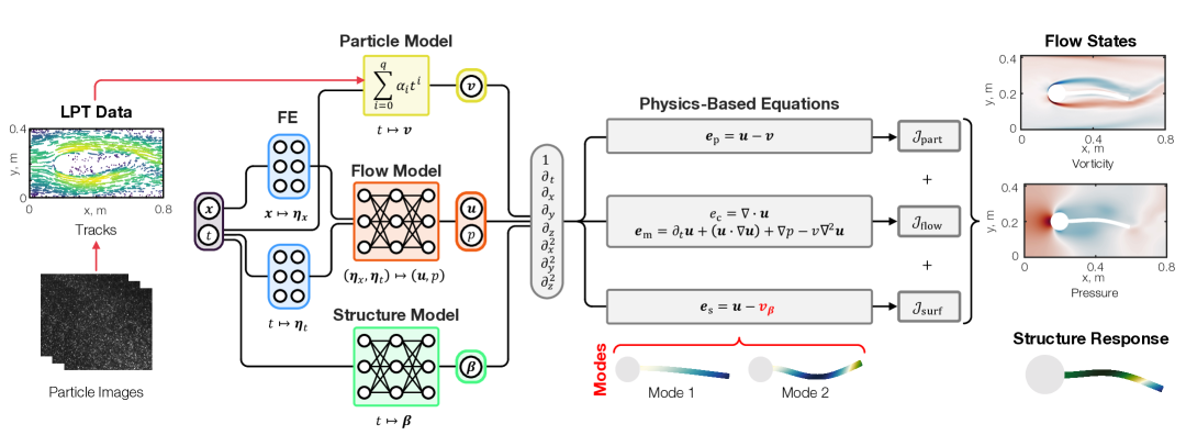
Figure 1: Architecture for FSI reconstruction: PINNs are used to model the flow and structure. Particle trajectories are imposed as hard constraints on the particle models, while soft constraints enforce the fluid’s governing equations and the moving-wall boundary condition.

The surface model, $\mathsf{S}$, represents a continuous 2D surface embedded in 3D space (or a 1D curve in 2D space) using a set of discrete mesh points, whose coordinates at time $t$ are collected in the vector $\boldsymbol{p}\in\partial\mathcal{V}_{t}$, which consists of points $\boldsymbol{x}\in\mathbb{R}^{d}$ that correspond to material points on the fluid–structure interface. The instantaneous surface position is approximated as the sum of a base surface, $\overline{\boldsymbol{p}}$, and a linear combination of $n_{\mathrm{m}}$ deflection/bending modes, $\boldsymbol{\Phi}=(\boldsymbol{\phi}_{1},\dots,\boldsymbol{\phi}_{n_{\mathrm{m}}})$, introduced formally in Sec. 2.3. The time-dependent modal coefficients are stored in the vector $\boldsymbol{\beta}\in\mathbb{R}^{n_{\mathrm{m}}}$, yielding a linear surface state of the form

$$\boldsymbol{p}\approx\overline{\boldsymbol{p}}+\boldsymbol{\Phi}\boldsymbol{\beta}.$$ (3)

The surface response is parameterized by a “solid PINN,” which maps time to the modal coefficients,

$$\mathsf{S}:\mathcal{T}\rightarrow\mathbb{R}^{n_{\mathrm{m}}},\quad t\mapsto\boldsymbol{\beta}.$$ (4)

Differentiating $\boldsymbol{\beta}$ with respect to time yields the surface velocity.

Lastly, measurements of particle positions are grouped into discrete “tracks,” each containing a sequence of positions for a single particle. The motion of the $k$th particle is described by a dedicated model, $\sdx{\mathsf{P}}[k]$, which maps time to that particle’s velocity,

$$\sdx{\mathsf{P}}[k]:\sdx{\mathcal{T}}[k]\rightarrow\mathbb{R}^{d},\quad t\mapsto\sdx{\boldsymbol{v}}[k]\quad\text{for}\quad k\in\{1,2,\dots,n_{\mathrm{p}}\},$$ (5)

where $\sdx{\boldsymbol{v}}[k]$ is the predicted velocity of the $k$th particle at time $t$, $\sdx{\mathcal{T}}[k]\subseteq\mathcal{T}$ is the time interval covered by the track, and $n_{\mathrm{p}}$ is the total number of particle tracks. For the model to be physically admissible, its output must satisfy the kinematic advection constraint, i.e., when integrated in time, the predicted velocity must reproduce the tracked particle positions. Section 2.4 describes how we embed this constraint directly into the structure of $\sdx{\mathsf{P}}[k]$.

2.1.2 Loss Terms

The flow, structure, and particle states, represented by $\mathsf{F}$, $\mathsf{S}$, and $\sdx{\mathsf{P}}[k]$, must satisfy the fluid’s governing equations, adhere to the moving-wall condition, and remain consistent with the measurements. As noted above, the agreement of $\sdx{\mathsf{P}}[k]$ with the LPT data is strictly enforced by its formulation. Flow equations and interface constraints, by contrast, are weakly enforced by minimizing a composite physics-based loss function that includes residuals from the governing equations and boundary conditions,

$$\mathscr{J}_{\mathrm{total}}=\gamma_{1}\,\mathscr{J}_{\mathrm{flow}}+\gamma_{2}\,\mathscr{J}_{\mathrm{surf}}+\gamma_{3}\,\mathscr{J}_{\mathrm{part}},$$ (6)

where $\gamma_{i}$ are weighting coefficients tuned to balance the contributions of the loss terms. The individual components, $\mathscr{J}_{\mathrm{flow}}$, $\mathscr{J}_{\mathrm{surf}}$, and $\mathscr{J}_{\mathrm{part}}$, encode the fluid’s governing equations, interface condition, and particle transport physics, respectively.

The flow physics loss is defined as

$$\mathscr{J}_{\mathrm{flow}}=\frac{\mathrm{dim}(\boldsymbol{e}_{\mathrm{f}})^{-1}}{\left|\Omega\right|}\iint_{\Omega}\left\lVert\boldsymbol{e}_{\mathrm{f}}\right\rVert_{2}^{2}\mathrm{d}\boldsymbol{x}\,\mathrm{d}t,$$ (7)

where $\boldsymbol{e}_{\mathrm{f}}\in\mathbb{R}^{d+1}$ contains the residuals of the incompressible continuity and Navier–Stokes equations,

$$e_{\mathrm{c}} =\nabla\cdot\boldsymbol{u},$$ (8a)

$$\boldsymbol{e}_{\mathrm{m}} =\frac{\partial\boldsymbol{u}}{\partial t}+\left(\boldsymbol{u}\cdot\nabla\right)\mathopen{}\boldsymbol{u}+\nabla p-\nu\nabla^{2}\boldsymbol{u},$$ (8b)

where $\nu$ is the kinematic viscosity and $\boldsymbol{e}_{\mathrm{f}}=(e_{\mathrm{c}},\boldsymbol{e}_{\mathrm{m}})$. Integration over $\Omega$ is interpreted in the Lebesgue sense, with $\mathrm{d}\boldsymbol{x}$ and $\mathrm{d}t$ indicating the standard Lebesgue measures $\mathrm{d}\mu(\boldsymbol{x})$ and $\mathrm{d}\mu(t)$. That is, $\mu(\mathcal{V}_{t})$ gives the spatial volume of the flow domain at time $t$ and $\mu(\mathcal{T})$ gives the total duration of the reconstruction interval. This convention is used throughout the paper.

The boundary loss is defined as

$$\mathscr{J}_{\mathrm{surf}}=\frac{\mathrm{dim}(\boldsymbol{e}_{\mathrm{s}})^{-1}}{|\partial\Omega|}\iint_{\partial\Omega}\left\lVert\boldsymbol{e}_{\mathrm{s}}\right\rVert_{2}^{2}\mathrm{d}\boldsymbol{x}\,\mathrm{d}t,$$ (9)

where $\partial\Omega$ is the space–time surface formed by the union of fluid–structure interfaces over $\mathcal{T}$,

$$\partial\Omega=\bigcup_{t\in\mathcal{T}}\partial\mathcal{V}_{t}\times\{t\}\subset\mathbb{R}^{d}\times\mathbb{R},$$ (10)

with $\partial\mathcal{V}_{t}$ being the portion of the flow domain boundary corresponding to the interface at time $t$. The residual vector $\boldsymbol{e}_{\mathrm{s}}$ quantifies the mismatch between the fluid velocity predicted by $\mathsf{F}$ and the surface velocity predicted by $\mathsf{S}$, evaluated at points $(\boldsymbol{x},t)\in\partial\Omega$. This term weakly enforces a no-slip condition along the moving solid surface.

A particle physics loss is introduced to couple the particle model, which encodes the LPT measurements, to the flow and structure models,

$$\mathscr{J}_{\mathrm{part}}=\frac{\mathrm{dim}\mathopen{}\left(\sdx{\boldsymbol{e}}[k][\mathrm{p}]\right)^{-1}}{n_{\mathrm{p}}}\sum_{k=1}^{n_{\mathrm{p}}}\left(\frac{1}{\left|\sdx{\mathcal{T}}[k]\right|}\int_{\sdx{\mathcal{T}}[k]}\left\lVert\sdx{\boldsymbol{e}}[k][\mathrm{p}]\right\rVert_{2}^{2}\mathrm{d}t\right),$$ (11)

where $\sdx{\boldsymbol{e}}[k][\mathrm{p}]$ is the residual vector associated with the governing equation for the $k$th particle. For tracer particles that passively follow the flow, the velocity of the particle is assumed to match the fluid velocity, i.e., $\boldsymbol{v}=\boldsymbol{u}$, yielding the residual

$$\sdx{\boldsymbol{e}}[k]=\boldsymbol{u}\mathopen{}\left[\sdx{\boldsymbol{x}}[k](t),t\right]-\sdx{\boldsymbol{v}}[k]\mathopen{}\left(t\right).$$ (12)

Here, $\sdx{\boldsymbol{v}}[k]$ is the particle velocity predicted by model $\sdx{\mathsf{P}}[k]$ and $\boldsymbol{u}$ is the fluid velocity from $\mathsf{F}$, evaluated at the corresponding particle position determined from $\sdx{\mathsf{P}}[k]$. This loss therefore couples the particle and fluid states. The framework can also accommodate large positional uncertainties and non-ideal tracer particles subject to inertial transport effects, as demonstrated in Refs. [32, 33].

The integrals in Eqs. (7), (9), and (11) cannot be evaluated in closed form, but they may be efficiently approximated using Monte Carlo sampling. Accurate integration requires a dynamic sampling scheme that accounts for the evolving spatial domains $\mathcal{V}_{t}$ and $\partial\mathcal{V}_{t}$, which are estimated using the transient surface shape from $\mathsf{S}$. Our sampling strategy and associated numerical considerations are described in Sec. 3. A data loss may also be included to account for measurement noise in the particle positions, which is particularly relevant for single-camera LPT modalities such as plenoptic imaging or digital in-line holography [33]. Joint minimization of $\mathscr{J}_{\mathrm{flow}}$, $\mathscr{J}_{\mathrm{surf}}$, and $\mathscr{J}_{\mathrm{part}}$ produces particle velocities that strictly match the experimental data, while yielding flow and structure states that approximately satisfy the governing equations and enforce the no-slip condition at the moving interface.

2.2 Flow Model

Flow states are represented by one or more coordinate neural networks in our framework. The generic architecture of these deep, feed-forward networks, $\mathsf{N}:\sdx{\boldsymbol{z}}[0]\mapsto\sdx{\boldsymbol{z}}[n_{\mathrm{L}}+1]$, includes an input layer, an output layer, and a sequence of $n_{\mathrm{L}}$ hidden layers,

$$\sdx{\boldsymbol{z}}[n_{\mathrm{L}}+1]=\mathsf{N}\mathopen{}\left(\sdx{\boldsymbol{z}}[0]\right)=\sdx{\boldsymbol{W}}[n_{\mathrm{L}}+1]\left[\sdx{\mathsf{L}}[n_{\mathrm{L}}]\circ\sdx{\mathsf{L}}[n_{\mathrm{L}}-1]\circ\dots\circ\sdx{\mathsf{L}}[2]\circ\mathsf{G}\mathopen{}\left(\sdx{\boldsymbol{z}}[0]\right)\right]+\sdx{\boldsymbol{b}}[n_{\mathrm{L}}+1],$$ (13a)

with hidden layers $$\sdx{\mathsf{L}}[l]:\sdx{\boldsymbol{z}}[l-1]\mapsto\sdx{\boldsymbol{z}}[l]$$ given by

$$\sdx{\boldsymbol{z}}[l]=\sdx{\mathsf{L}}[l]\mathopen{}\left(\sdx{\boldsymbol{z}}[l-1]\right)=\mathrm{swish}\mathopen{}\left(\sdx{\boldsymbol{W}}[l]\sdx{\boldsymbol{z}}[l-1]+\sdx{\boldsymbol{b}}[l]\right)\quad\text{for}\quad l\in\{2,3,\dots,n_{\mathrm{L}}\}.$$ (13b)

Here, $\sdx{\boldsymbol{z}}[l]$ contains the values of neurons in the $l$th layer, $\sdx{\boldsymbol{W}}[l]$ and $\sdx{\boldsymbol{b}}[l]$ are the corresponding weight matrix and bias vector, and the symbol $\circ$ indicates a function composition. Swish activations are used in all hidden layers, defined element-wise as

$$\mathrm{swish}(z)=\frac{z\,\exp(z)}{1+\exp(z)}.$$ (14)

These activations are known to improve gradient flow in coordinate neural networks compared to alternatives such as the hyperbolic tangent [34]. To mitigate the spectral bias of training by gradient descent [35], the first hidden layer, $\sdx{\mathsf{L}}[1]$, is replaced with a Fourier encoding [36],

$$\sdx{\boldsymbol{z}}[1]=\mathsf{G}\mathopen{}\left(\sdx{\boldsymbol{z}}[0]\right)=\left[\sin\mathopen{}\left(2\pi\boldsymbol{f}_{1}\cdot\sdx{\boldsymbol{z}}[0]\right),\,\cos\mathopen{}\left(2\pi\boldsymbol{f}_{1}\cdot\sdx{\boldsymbol{z}}[0]\right),\dots,\,\sin\mathopen{}\left(2\pi\boldsymbol{f}_{n_{\mathrm{F}}}\cdot\sdx{\boldsymbol{z}}[0]\right),\,\cos\mathopen{}\left(2\pi\boldsymbol{f}_{n_{\mathrm{F}}}\cdot\sdx{\boldsymbol{z}}[0]\right)\right],$$ (15)

where $\boldsymbol{f}_{j}$ is a vector of random frequencies assigned to each input dimension and $n_{\mathrm{F}}$ is the number of Fourier features. The frequencies are drawn from a zero-mean Gaussian distribution before training and fixed thereafter. The standard deviation of the frequency distribution controls the spectral bandwidth of functions that the network can easily represent [36].

While a single network can effectively learn vector-valued functions with components of similar spectral content, it becomes less efficient when those components exhibit distinct spectral characteristics. In turbulent flows, for instance, velocity and pressure fields often have different energy spectra. Using separate networks for $\boldsymbol{u}$ and $p$ can therefore improve reconstruction accuracy while minimizing the number of trainable parameters. We thus use dedicated velocity and pressure networks, $\mathsf{F}_{\boldsymbol{u}}:(\boldsymbol{x},t)\mapsto\boldsymbol{u}$ and $\mathsf{F}_{p}:(\boldsymbol{x},t)\mapsto p$, each following the architecture in Eq. (13). Automatic differentiation of these networks is used to evaluate the residuals in Eq. (8).

2.3 Structure Model

Representing time-varying geometries is a fundamental challenge in flow reconstruction and inverse design problems involving FSI. The fluid–solid interface $\partial\mathcal{V}_{t}$ may undergo large and complex deformations, and our goal is to infer its shape over time from sparse measurements, such as particle tracks or MRV data. Since both the surface and surrounding flow field are, in principle, infinite-dimensional, recovering them from limited observations is a high-dimensional, ill-posed inverse problem. To regularize reconstructions, we adopt a low-dimensional modal representation of the surface geometry. In this approach, the instantaneous surface is approximated as a linear combination of deformation modes. These modes are obtained from either a (i) physics-based eigenmode analysis or (ii) data-driven analysis of surface measurements. In both cases, the modal expansion yields a compact, physically interpretable basis for representing shape dynamics.

We treat the evolving interface $\partial\mathcal{V}_{t}$ as a smooth $(d-1)$-dimensional manifold that is embedded in $\mathbb{R}^{d}$ [37, 38]. Due to possible curvature and a complex topology, a global chart from $\mathcal{V}_{t}$ to this surface is generally unavailable. Instead, we define an atlas of local charts,

$$\mathcal{A}=\left\{\left(\sdx{\Theta}[i],\sdx{\mathsf{M}}[i]\right)\mid i\in\mathcal{I}\right\},$$ (16)

where $\sdx{\Theta}[i]\subset\mathbb{R}^{d-1}$ is a domain of local coordinates on the surface and $\sdx{\mathsf{M}}[i]:\sdx{\Theta}[i]\times\mathcal{T}\rightarrow\partial\mathcal{V}_{t}$ defines a smooth, time-dependent embedding of a surface patch. The full surface is given by the union

$$\partial\mathcal{V}_{t}=\bigcup_{i\in\mathcal{I}}\left\{\sdx{\mathsf{M}}[i](\boldsymbol{\theta},t)\mid\boldsymbol{\theta}\in\sdx{\Theta}[i]\right\}.$$ (17)

Each chart is assumed to be regular and locally injective, ensuring that the surface is non-degenerate and free of self-intersections within each patch. We also assume the existence of a local inverse, $\sdx{\mathsf{M}}[i]{{}^{-1}}:\Omega\rightarrow\mathbb{R}^{d-1}$, which maps spatial points back to material coordinates, $(\boldsymbol{x},t)\mapsto\boldsymbol{\theta}$. This framework provides a stable coordinate system anchored to material points on the solid surface, though it does not accommodate geometric singularities or topological changes such as merging or tearing.

To construct a modal basis using a proper orthogonal decomposition (POD), we define a global parameter space by the disjoint union

$$\Theta=\bigsqcup_{i\in\mathcal{I}}\sdx{\Theta}[i],$$ (18)

and we assume smooth blending through a partition of unity [39]. The mapping $\mathsf{M}:\Theta\times\mathcal{T}\rightarrow\mathbb{R}^{d}$ provides global surface coordinates, enabling us to define mean and fluctuating positions on the surface as

$$\overline{\boldsymbol{x}}(\boldsymbol{\theta}) =\frac{1}{|\mathcal{T}|}\int_{\mathcal{T}}\mathsf{M}(\boldsymbol{\theta},t)\,\mathrm{d}t,$$ (19a)

$$\delta\boldsymbol{x}(\boldsymbol{\theta},t) =\mathsf{M}(\boldsymbol{\theta},t)-\overline{\boldsymbol{x}}(\boldsymbol{\theta}).$$ (19b)

To obtain a modal representation of coherent deformation patterns for the surface, we define the surface displacement covariance kernel [40, 41],

$$\mathsf{K}(\boldsymbol{\theta},\boldsymbol{\theta}^{\prime})=\frac{1}{\left|\mathcal{T}\right|}\int_{\mathcal{T}}\delta\boldsymbol{x}(\boldsymbol{\theta},t)\cdot\delta\boldsymbol{x}(\boldsymbol{\theta}^{\prime},t)\,\mathrm{d}t,$$ (20)

and solve the associated eigenproblem,

$$\int_{\Theta}\mathsf{K}(\boldsymbol{\theta},\boldsymbol{\theta}^{\prime})\,\boldsymbol{\varphi}_{j}(\boldsymbol{\theta}^{\prime})\,\mathrm{d}\boldsymbol{\theta}^{\prime}=\lambda_{j}\,\boldsymbol{\varphi}_{j}(\boldsymbol{\theta}).$$ (21)

The resulting orthonormal modes, $\boldsymbol{\varphi}_{k}:\Theta\rightarrow\mathbb{R}^{d}$, satisfy

$$\int_{\Theta}\boldsymbol{\varphi}_{j}(\boldsymbol{\theta})\cdot\boldsymbol{\varphi}_{k}(\boldsymbol{\theta})\,\mathrm{d}\boldsymbol{\theta}=\delta_{jk}.$$ (22)

We define a truncated modal expansion,

$$\delta\mathbf{x}(\boldsymbol{\theta},t)\approx\sum_{j=1}^{n_{\mathrm{m}}}\beta_{j}(t)\,\boldsymbol{\varphi}_{j}(\boldsymbol{\theta}),$$ (23)

with $n_{\mathrm{m}}$ modes that are paired with time-dependent coefficients,

$$\beta_{j}(t)=\int_{\Theta}\delta\mathbf{x}(\boldsymbol{\theta},t)\cdot\boldsymbol{\varphi}_{j}(\boldsymbol{\theta})\,\mathrm{d}\boldsymbol{\theta}.$$ (24)

Given an appropriate choice of $n_{\mathrm{m}}$, this continuous representation yields a mathematically well-posed framework for analyzing surface dynamics and underpins our discrete implementation.

In practice, both the base surface and deformation modes are evaluated at a discrete set of nodal positions $\{\sdx{\boldsymbol{\theta}}[1],\dots,\sdx{\boldsymbol{\theta}}[n_{\mathrm{s}}]\}$, which define a material mesh over the deforming boundary $\partial\mathcal{V}_{t}$. The corresponding physical positions $\sdx{\boldsymbol{x}}[i]\in\mathbb{R}^{d}$ are stacked into a global vector $\boldsymbol{p}\in\mathbb{R}^{dn_{\mathrm{s}}}$. The (time-averaged) base surface is given by $\overline{p}_{(i-1)d+j}=\overline{x}_{j}(\sdx{\boldsymbol{\theta}}[i])$ and the mode matrix is defined by $\Phi_{ij}=[\boldsymbol{\varphi}_{j}(\sdx{\boldsymbol{\theta}}[k])]_{\ell}$, where the row index is $i=(k-1)\,d+\ell$. Surface motion is governed by the solid PINN $\mathsf{S}$, configured according to Eq. (13), which outputs time-dependent modal coefficients $\boldsymbol{\beta}$. The resulting surface at time $t$ is approximated as

$$\boldsymbol{p}(t)=\overline{\boldsymbol{p}}+\boldsymbol{\Phi}\boldsymbol{\beta}(t),$$

with the corresponding surface velocity obtained by automatic differentiation of $\mathsf{S}$ with respect to $t$,

$$\frac{\mathrm{d}\boldsymbol{p}}{\mathrm{d}t}=\boldsymbol{\Phi}\frac{\mathrm{d}\boldsymbol{\beta}}{\mathrm{d}t}.$$ (25)

This velocity provides the kinematic boundary condition needed to evaluate the surface loss term in Eq. (9). The modal basis $\boldsymbol{\Phi}$ may be constructed a priori through a finite element analysis using estimated material properties or extracted a posteriori by applying a modal decomposition to time-resolved surface tracking data (i.e., in multi-modal FSI experiments or using asynchrynous surface data). Both strategies are demonstrated using synthetic benchmarks in Sec. 5.

2.4 Particle Track Model

We define a kinematics-constrained model $\sdx{\mathsf{P}}[k]$ for each particle track, which maps time to the particle’s velocity while satisfying an advection constraint,

$$\frac{\mathrm{d}\sdx{\boldsymbol{x}}[k]}{\mathrm{d}t}=\sdx{\boldsymbol{v}}[k]\;\Longrightarrow\;\sdx{\boldsymbol{x}}[k][j+1]-\sdx{\boldsymbol{x}}[k][j]=\int_{t_{j}}^{t_{j+1}}\sdx{\boldsymbol{v}}[k]\mathopen{}\left(t\right)\mathrm{d}t,$$ (26)

where $\sdx{\boldsymbol{x}}[k]$ and $\sdx{\boldsymbol{v}}[k]$ are the $k$th particle’s position and velocity and $j$ indexes the time steps. Each track comprises a sequence of $n_{k}$ positions, $\sdx{\boldsymbol{x}}[k][j]$, recorded at discrete times ${t_{j}}$. To enable efficient gradient-based optimization, we embed this constraint into the model using the theory of functional connections [42], which reformulates the constrained problem in terms of unconstrained parameters. We adopt a projection–switch form for the velocity model,

$$\mathsf{P}\mathopen{}\left(t\right)\equiv v\mathopen{}\left(t\right)=g\mathopen{}\left(t\right)+\sum_{j=1}^{n_{\mathrm{c}}}\eta_{j}\,\xi_{j}\mathopen{}\left(t\right).$$ (27)

where $v$ is one component of the particle’s velocity vector, $g$ is a freely chosen function with tunable parameters, and $\eta_{j}$ and $\xi_{j}$ are projection coefficients and switch functions, respectively, which enforce the integral constraints over each time interval $[t_{j-1},t_{j}]$. The number of constraints is $n_{\mathrm{c}}=n_{k}-1$, where $n_{k}$ is the number of position measurements in the $k$th track. A separate copy of this model is used for each spatial dimension, and the track index $k$ is omitted here for brevity.

The free function is chosen as a $q$th-order polynomial,

$$g\mathopen{}\left(t\right)=\sum_{i=0}^{q}\alpha_{i}\,t^{i},$$ (28)

with trainable coefficients $\alpha_{i}$. To enforce the advection constraint, we define the projection coefficients as

$$\eta_{j}=\left(x_{j}-x_{j-1}\right)-\int_{t_{j-1}}^{t_{j}}g\mathopen{}\left(t\right)\mathrm{d}t.$$ (29)

which encodes the shifts needed for $g$ to match the observed displacements over each interval. These corrections are applied using a set of switch functions,

$$\xi_{j}\mathopen{}\left(t\right)=\sum_{i=1}^{n_{\mathrm{c}}}h_{i}\mathopen{}\left(t\right)L_{ij},$$ (30)

where $h_{i}(t)=t^{i-1}$ are monomial support functions and and $L_{ij}$ are entries of a weight matrix $\boldsymbol{L}$. This matrix is chosen so that the switch functions $\xi_{j}$ integrate to unity over the corresponding time intervals and vanish elsewhere, which is enforced by requiring that

$$\boldsymbol{HL}=\boldsymbol{I},$$ (31)

where $\boldsymbol{H}$ is defined by

$$H_{ij}=\int_{t_{i-1}}^{t_{i}}h_{j}\mathopen{}\left(t\right)\mathrm{d}t,$$ (32)

The use of monomial basis functions ensures that $\boldsymbol{H}$ is invertible, guaranteeing a unique solution for $\boldsymbol{L}$.

Given the free function $g$ and a particle track, a closed-form expression for the velocity polynomial can be derived in two steps: (1) compute the projection coefficients $\boldsymbol{\eta}$ via Eq. (29), then (2) determine $\boldsymbol{L}$ by solving Eq. (31) to specify the switch functions $\boldsymbol{\xi}$. A compact matrix expression for the velocity follows from the preceding expressions,

$$v\mathopen{}\left(t\right)=\left[\boldsymbol{\alpha}^{\top}\left(\boldsymbol{I}-\boldsymbol{C}\widehat{\boldsymbol{L}}\right)+\boldsymbol{\delta}^{\top}\widehat{\boldsymbol{L}}\right]\boldsymbol{\tau}\mathopen{}\left(t\right),$$ (33)

where $\boldsymbol{\tau}(t)=\{t^{j}\mid j=0,\dots,p\}$ is a time vector, $\boldsymbol{\updelta}=\{x_{j}-x_{j-1}\mid j=1,\dots,n_{\mathrm{c}}\}$ is a displacement vector, and $\boldsymbol{C}$ is a support matrix with elements

$$C_{ij}=i^{-1}\left(t_{j}^{i}-t_{j-1}^{i}\right).$$ (34)

In these expressions, $t_{j}^{i}$ is the time $t_{j}$ raised to the $i$th power and $\widehat{\boldsymbol{L}}=[\boldsymbol{L};\mathbf{0}]^{\top}$ is an $n_{\mathrm{c}}\times(p+1)$ augmented weight matrix. This velocity model is differentiable and satisfies the advection constraint for any set of coefficients $\boldsymbol{\alpha}\in\mathbf{R}^{q}$, making it well suited for gradient-based optimization.

Integrating $v$ yields a continuous particle trajectory,

$$x\mathopen{}\left(t\right)=\left[\boldsymbol{\alpha}^{\top}\left(\boldsymbol{I}-\boldsymbol{C}\widehat{\boldsymbol{L}}\right)+\boldsymbol{\delta}^{\top}\widehat{\boldsymbol{L}}\right]\widetilde{\boldsymbol{\tau}}\mathopen{}\left(t\right)+x_{0},$$ (35)

where $x_{0}$ is the initial particle position and the position time vector is $\widetilde{\boldsymbol{\tau}}(t)=\{t^{j+1}/(j+1)\mid j=0,\dots,p\}$. This formulation enables efficient, differentiable evaluation of particle positions and velocities at arbitrary times $t\in\sdx{\mathcal{T}}[k]$, and it is used to compute the particle loss $\mathscr{J}_{\mathrm{part}}$ in Eq. (11).

3 Approximating Loss Terms for Dynamic Domains

To train the fluid, structure, and particle models, we minimize a composite loss functional $\mathscr{J}_{\mathrm{total}}$ defined in terms of residuals over continuous space–time volumes and surfaces. These residuals arise from the fluid’s governing equations, inter-phase boundary conditions, and particle transport equations, and they are integrated over the transient fluid domain $\Omega$, fluid–structure interface $\partial\Omega$, and time intervals of the particle tracks $\sdx{\mathcal{T}}[k]$. Explicit expressions for the loss terms are given in Eqs. (7), (9), and (11). Since the integrals cannot be evaluated in closed form, we approximate them via Monte Carlo sampling,

$$\mathscr{J}=\frac{1}{|\Omega|}\iint_{\Omega}\mathscr{L}\mathopen{}\left(\boldsymbol{x},t\right)\mathrm{d}\boldsymbol{x}\,\mathrm{d}t\approx\frac{1}{N}\sum_{i=1}^{N}\mathscr{L}\mathopen{}\left(\sdx{\boldsymbol{x}}[i],\sdx{t}[i]\right)$$ (36)

which holds for large $N$, where $\mathscr{L}$ is a squared residual term and $(\sdx{\boldsymbol{x}}[i],\sdx{t}[i])$ are random samples drawn from the relevant domain. The integrals are defined with respect to Lebesgue measures on $\Omega$, $\partial\Omega$, and $\sdx{\mathcal{T}}[k]$, so our sampling scheme is constructed to approximate uniform coverage with respect to those measures. Time samples are drawn uniformly from the reconstruction interval $\mathcal{T}$ or track segment $\sdx{\mathcal{T}}[k]$, and spatial samples are allocated in proportion to the length (1D), area (2D) or volume (3D) of subregions of $\mathcal{V}_{t}$ or $\partial\mathcal{V}_{t}$. This treatment ensures consistency between the sampling distribution and the continuous measure in each loss term. Fluid, structure, and particle residuals ($\boldsymbol{e}_{\mathrm{f}}$, $\boldsymbol{e}_{\mathrm{s}}$, and $\sdx{\boldsymbol{e}}[k][\mathrm{p}]$) come from the corresponding governing equations or boundary conditions, which are evaluated using the fluid, structure, and particle models. The gradient of the total loss is then computed by automatic differentiation and used in backpropagation to update all the model parameters.

The effectiveness of this approach depends on the accuracy of the sampling scheme [43, 44, 45, 46]. A poor sampling strategy introduces variance in the integral approximations, leading to noisy gradients and degraded convergence behavior [47]. We therefore implement a dynamic sampling strategy that tracks the evolving geometry of the fluid and structure domains. This ensures that each loss term is a faithful approximation of its ideal, continuous counterpart and that the learned model outputs approach a weak-form solution to the governing equations and boundary conditions. We briefly outline the sampling strategy for each loss term below, with reference to the 2D and 3D FSI geometries tested in this work, though we defer the complete definitions of these cases to Sec. 4.

3.1 Fluid Domain Sampling

The fluid domain is partitioned into subregions based on their proximity to solid boundaries and their geometric complexity. As illustrated in Fig. 2 for the 2D flapping-plate case (see Sec. 4.1.1), we define three types of subdomains: (1) fixed far-field rectangles (blue), (2) rectangular regions containing a circular cutout around the rigid cylinder (green), and (3) a deforming near-field region adjacent to the flapping plate, discretized by a triangular mesh (red). The far-field regions do not interact with the structure, whereas the near-field regions interface with either rigid or compliant boundaries. Sampling is performed at randomly selected time instants $t\in\mathcal{T}$, drawn uniformly over the time horizon. At each instant, spatial locations $\boldsymbol{x}\in\mathcal{V}_{t}$ are sampled from each subregion in proportion to its area (2D) or volume (3D), yielding uniform coverage of the time-dependent fluid domain. In axis-aligned rectangular regions, we use independent uniform distributions over each coordinate axis. For circular cutouts, samples are drawn from the bounding rectangle and points falling within the cutout are rejected.

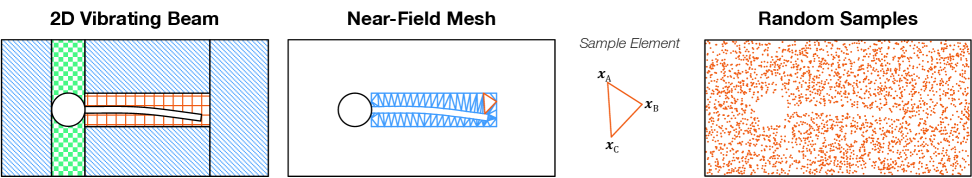
Figure 2: Sampling strategy for the fluid loss: (left) the fluid domain is partitioned into far-field regions (blue), near-field regions adjacent to rigid structures (green), and near-field regions about the compliant structure (red). (middle) The near-field region around the compliant surface is discretized into elements anchored to surface nodes $\boldsymbol{p}$. (right) Samples are drawn from each subregion in proportion to its area, producing uniform spatial coverage of $\mathcal{V}_{t}$.

The deforming near-field region is handled via mesh-based sampling. At each sampled time, the surface mesh is updated based on predicted mode coefficients $\boldsymbol{\beta}$ from $\mathsf{S}$, deforming the base shape accordingly. In 2D, triangular elements are sampled with probability proportional to their area; in 3D, the elements are tetrahedra and weighted by instantaneous volume. Within each element, random points are generated using barycentric coordinates [48]. For a triangle with vertices $\boldsymbol{x}_{\mathrm{A}}$, $\boldsymbol{x}_{\mathrm{B}}$, and $\boldsymbol{x}_{\mathrm{C}}$, per Fig. 2, we set

$$\boldsymbol{x}=(1-\sqrt{r_{1}})\,\boldsymbol{x}_{\mathrm{A}}+r_{1}\,(1-r_{2})\,\boldsymbol{x}_{\mathrm{B}}+\sqrt{r_{1}}r_{2}\,\boldsymbol{x}_{\mathrm{C}},$$

where $$r_{1},r_{2}\sim\mathcal{U}(0,1) \boldsymbol{x}_{\mathrm{D}}$$. The 3D equivalent, with an added vertex , uses

$$\boldsymbol{x}=(1-\sqrt[3]{r_{1}})\,\boldsymbol{x}_{\mathrm{A}}+\sqrt[3]{r_{1}}(1-\sqrt{r_{2}})\,\boldsymbol{x}_{\mathrm{B}}+\sqrt[3]{r_{1}}\sqrt{r_{2}}(1-r_{3})\,\boldsymbol{x}_{\mathrm{C}}+\sqrt[3]{r_{1}}\sqrt{r_{2}}r_{3}\,\boldsymbol{x}_{\mathrm{D}},$$

The mesh is not used for numerical discretization but serves as a flexible partition to efficiently support closed-form spatial sampling.

In the 3D flexible pipe flow case (see Sec. 4.1.2), the flow domain is entirely enclosed by the structure. Here, we sample directly from a tetrahedral mesh that evolves over time with nodal motion given by $\boldsymbol{\beta}$. As in 2D, element volumes determine sampling probabilities, and barycentric sampling is used to generate spatial points consistent with the instantaneous geometry.

3.2 Structure Surface Sampling

To evaluate the boundary loss, we sample points from the deforming structure surface $\partial\mathcal{V}_{t}$, discretized into line segments or triangles, depending on $d$. Segment endpoints and triangle vertices are updated at each frame from the structure prediction $\boldsymbol{p}$. Sampling along line segments is done via uniform interpolation,

$$\boldsymbol{x}=(1-r)\,\boldsymbol{x}_{\mathrm{A}}+r\boldsymbol{x}_{\mathrm{B}},$$

with $r_{i}\sim\mathcal{U}(0,1)$; the associated velocity is also linearly interpolated,

$$\boldsymbol{v}_{\boldsymbol{\beta}}(\boldsymbol{x})=(1-r)\,\boldsymbol{v}_{\boldsymbol{\beta}}\mathopen{}\left(\boldsymbol{x}_{\mathrm{A}}\right)+r\boldsymbol{v}_{\boldsymbol{\beta}}\mathopen{}\left(\boldsymbol{x}_{\mathrm{B}}\right).$$

For 2D surfaces abutting 3D flows, we apply barycentric sampling using the same weights as in the 2D fluid domain elements, and we interpolate the surface velocity accordingly. In addition, for the 2D test case with a fixed circular solid boundary, we uniformly sample points along the circle to enforce the no-slip condition. These fixed-boundary samples remain constant in time and ensure that the velocity satisfies the zero-wall condition throughout training.

3.3 Particle Track Sampling

The particle physics loss is evaluated along a batch of randomly selected tracks. Each track is defined over a measurement interval $\sdx{\mathcal{T}}[k]$. For a random selection of particles, we draw random times $t\in\sdx{\mathcal{T}}[k]$. Positions and velocities at these time are computed from the trajectory models $\sdx{\mathsf{P}}[k]$, and the corresponding fluid velocities are determined via $\mathsf{F}$. The loss is evaluated based on local discrepancies between particle and fluid velocities from $\sdx{\mathsf{P}}[k]$ and $\mathsf{F}$.

4 Flow Cases and Implementation Details

We evaluate our reconstruction framework on two benchmark FSI problems: (1) a 2D vortex-induced flow over a flexible beam (a.k.a. “flapping-plate flow”) and (2) a 3D pulsatile flow through a flexible pipe (a.k.a. “flexi-pipe flow”). Ground truth data are generated from FSI simulations and synthetic particle tracks are obtained by advecting Lagrangian tracers according to the resulting velocity fields.

4.1 FSI Simulations

4.1.1 2D Flapping-Plate Flow

The first test case is a classical benchmark for 2D FSI, featuring vortex-induced vibrations of a flexible plate (or beam) affixed to the rear of a cylindrical bluff body within a confined channel [49]. This configuration is widely used to validate FSI solvers due to the presence of strong two-way coupling and large structural deformations. The fluid domain is a channel measuring 2.5 m in length and 0.41 m in height. A rigid cylinder of radius 0.05 m is fixed at the vertical midpoint $(0.2~\text{m},0.2~\text{m})$, and a linearly elastic beam of length 0.35 m and thickness 0.02 m is attached downstream. The beam is modeled with a Young’s modulus of $E_{\mathrm{s}}=5.6$ MPa, Poisson’s ratio of 0.4, and density of $\rho_{\mathrm{s}}=1000$ kg/m³. Fluid enters the channel from the left with a fully developed laminar velocity profile and a mean speed of 2 m/s, resulting in a Reynolds number of approximately 200 based on the cylinder diameter. The inlet velocity is ramped up using a step function, and a Gaussian perturbation is introduced at $t=1.5$ s to trigger vortex shedding. A stress-free condition is imposed at the outlet.

The simulation is conducted in COMSOL Multiphysics 5.6 using an ALE formulation. Fluid tractions along the beam induce structural motion, which feeds back to the fluid through a moving-wall boundary condition. The computational mesh consists of 5856 elements, with unstructured triangles around the cylinder and plate to resolve boundary layers and wake dynamics; structured quadrilateral elements are used downstream of the plate. We use second-order Lagrange elements for both velocity and pressure. Time integration is performed using a second-order backward differentiation formula, with a fixed time step of $\Delta t=0.05$ s. Stabilization is provided by the streamline upwind Petrov–Galerkin method, and the system is solved using a fully coupled Newton method with Anderson acceleration (damping factor 0.9, Jacobian updated once per step). The simulation runs for 5 s, with outputs recorded at 0.05 s intervals. Following flow destabilization, the beam undergoes sustained oscillations. Vertical tip displacements reach 34 mm at approximately 5.3 Hz, while horizontal oscillations are smaller at 2.7 mm near 11 Hz. Mean drag and lift forces are about 457 N and 2 N, respectively, with amplitudes of roughly 23 N and 150 N, which are in line with values reported in prior studies [49].

4.1.2 3D Flexi-Pipe Flow

In the second test case we simulate internal pulsatile flow through a compliant, straight-walled cylindrical vessel to mimic large-vessel hemodynamics [50]. The setup features two-way coupling between pressure-driven flow and structural wall deformation, resulting in pulse-wave propagation. The computational domain is a 10 cm long pipe with an inner radius of 1 cm (the fluid lumen) and an outer radius of 1.2 cm (the solid vessel wall). The lumen is discretized with 204,705 tetrahedral elements and the wall with 85,220 elements. The vessel wall is modeled as a homogeneous, isotropic, nearly incompressible neo-Hookean solid with density $\rho_{\mathrm{s}}=1$ g/cm³, Young’s modulus $E_{\mathrm{s}}=10^{7}$ dyn/cm², and Poisson’s ratio of 0.3. The fluid is assumed to be incompressible and Newtonian, with a constant density of $\rho=1$ g/cm³ and dynamic viscosity of $\mu=0.004$ Pa s. A no-slip condition is enforced across the fluid–structure interface. The initial condition is quiescent. A step increase in pressure of 5 kPa is applied at the inlet at $t=0$ s to initiate flow, while stress-free boundary conditions are applied at the outlet and on the exterior wall. Axial displacements of the wall are constrained to zero.

Simulations are carried out using SimVascular [51], which also uses an ALE-based solver to handle two-way coupled FSI. The fluid and solid subproblems are solved sequentially at each time step. Structural dynamics are integrated using the generalized-$\alpha$ method, and the fluid equations use a second-order time discretization. The coupled nonlinear system is solved using the generalized minimal residual method with an incomplete LU preconditioner and threshold-based filtering. Mesh motion in the fluid domain is computed via harmonic extension of the wall displacement. The simulation is run for 0.02 s, and synthetic measurements are generated over the first 0.012 s, during which the pressure wave propagates almost completely through the domain.

4.2 Synthetic Particle Track Generation

To simulate LPT measurements, we generate synthetic tracks that replicate key features of real-world experimental data, including those produced by advanced reconstruction algorithms such as Shake-The-Box [52]. Massless tracer particles of negligible size are uniformly seeded within the fluid domain and advected according to the simulated velocity field. Particle trajectories are computed using second-order Runge–Kutta integration, matching the time-stepping used in the flow solver. A periodic boundary condition is applied at the outlet, and particles that encounter solid boundaries are terminated and replaced by newly seeded tracers at the inlet. Tracks with fewer than five time steps are discarded to reflect practical detection and tracking limits commonly encountered in experiments.

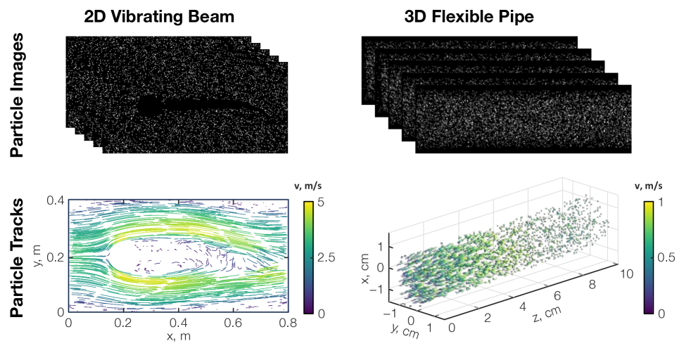
Figure 3: Synthetic particle tracks and images: (left) 2D flapping-plate case and (right) 3D flexible-pipe case. Particles are colored by instantaneous velocity magnitude. Note the sparse track density near the moving surfaces, which challenges direct inference of near-wall motion.

Figure 3 presents representative synthetic images and reconstructed particle tracks for both the 2D and 3D test cases. In the 2D flapping-plate flow, particles are seeded at the inlet. We initialize 4000 tracers uniformly throughout $\mathcal{V}_{0}$ and advect them over 700 time steps using a sampling interval of $\Delta t=0.05$ s. This setup corresponds to an effective particle density of approximately 0.004 particles-per-pixel (ppp), assuming imaging with a 1 MP camera operating at 20 Hz. These values fall well within achievable experimental parameters for planar LPT. To maintain a consistent particle density, terminated tracks (e.g., due to wall contact) are immediately replaced. The same methodology is used for the 3D flexi-pipe flow. A total of 10,000 tracers are initialized uniformly throughout the lumen and advected for 120 frames. This configuration yields a particle density of approximately 0.01 ppp, assuming a multi-camera setup with 1 MP sensors operating at 10 kHz for 0.012 s. As in the 2D case, tracers that contact the vessel wall are removed and re-injected at the inlet to maintain sampling density throughout the simulation.

4.3 Network Architecture and Training Protocol

The governing flow field satisfies the incompressible Navier–Stokes equations, forming the physics residuals $\boldsymbol{e}_{\mathrm{f}}$ in the fluid domain $\mathcal{V}_{t}$, per Eq. (7). At the fluid–structure interface $\partial\mathcal{V}_{t}$, we impose a moving-wall boundary condition in weak form, yielding residuals $\boldsymbol{e}_{\mathrm{s}}$ in Eq. (9). For particle tracking, we assume purely advective motion, so the Lagrangian residuals for each particle track are given by $\sdx{\boldsymbol{e}}[k][\mathrm{p}]=\boldsymbol{u}-\sdx{\boldsymbol{v}}[k]$, as defined in Eq. (11). The model includes four sets of trainable parameters, those of the velocity network $\mathsf{F}_{\boldsymbol{u}}$, pressure network $\mathsf{F}_{p}$, structure network $\mathsf{S}$, and particle kinematics models $\sdx{\mathsf{P}}[k]$. The velocity and pressure networks share a common architecture, with six hidden layers of 100 neurons each. The structure network uses four hidden layers with 150 neurons per layer. To improve expressivity, we use Fourier encodings with 256 features. For the 2D case, spatial input frequencies are sampled from a zero-mean Gaussian distribution with a standard deviation of 0.2, and we use a standard deviation of 0.8 for time. In the 3D case, a standard deviation of 0.2 is used for all frequencies. Network weights are initialized from a standard normal distribution, with biases set to zero at the start. Loss component weightings are chosen via a coarse grid search and remain fixed during training.

For each training iteration in the 2D case, 2000 samples are drawn from the fluid domain $\Omega$: 1800 from the fixed subregions and 200 from the dynamic near-field mesh, all sampled across 25 randomly chosen time frames. For the surface loss, 400 boundary points are sampled from $\partial\mathcal{V}_{t}$ per time step over 25 frames, yielding 5000 points per iteration. For the particle loss, we first select 5000 tracks, sampled with probabilities proportional to track length. From each selected track, 10 random times $t\in\sdx{\mathcal{T}}[k]$ are drawn, and the corresponding positions are computed using $\sdx{\mathsf{P}}[k]$ via Eq. (35). In the 3D flexi-pipe case, we use 5000 points from the fluid volume, 5000 from the structure boundary, and 5000 samples drawn from tracks, each sampled at 10 time frames. A detailed discussion of these sampling parameter choices is presented in Sec. 5.4. All model parameters are updated using the Adam optimizer with a fixed learning rate of $10^{-3}$. Training is conducted until convergence, requiring approximately $2\times 10^{5}$ iterations for the 2D case and $10^{5}$ iterations for the 3D case. The framework is implemented in TensorFlow 2.10 and executed on an NVIDIA GeForce RTX 3090 GPU. The total training time is about 5.5 hours for the 2D case and 1.5 hours for the 3D flexi-pipe reconstruction.

5 Results

Fluid–structure interactions are reported for two synthetic LPT tests designed to mimic real experiments. In both cases, our solver is only given the LPT data and surface modes. Reconstructions are compared to the CFD outputs to assess the accuracy of our method.

5.1 Modal Representations

Our framework employs a modal representation of the deforming surface $\partial\mathcal{V}_{t}$. A surface mesh is represented by a vector of nodal positions $\boldsymbol{p}$, which is decomposed into a base structure $\overline{\boldsymbol{p}}$ and time-dependent deformation field $\boldsymbol{p}^{\prime}(t)=\boldsymbol{p}(t)-\overline{\boldsymbol{p}}$, as described in Sec. 2.3. Surface deformations are approximated in a low-dimensional subspace, $\boldsymbol{p}^{\prime}(t)\approx\boldsymbol{\Phi}\boldsymbol{\beta}(t)$, where the columns of $\boldsymbol{\Phi}$ are spatial deformation modes and $\boldsymbol{\beta}$ is a vector of modal coefficients outputted by $\mathsf{S}$. We consider two strategies for constructing the modal basis, using a physics-based eigenmode analysis to compute modes in the 2D case and a data-driven method based for the 3D scenario. Both modal bases provide a compact yet expressive representation of the surface kinematics, reducing the structure model to a small number of degrees of freedom and facilitating accurate reconstructions of FSI. Leading modes for the 2D and 3D structures are shown in Fig. 4.

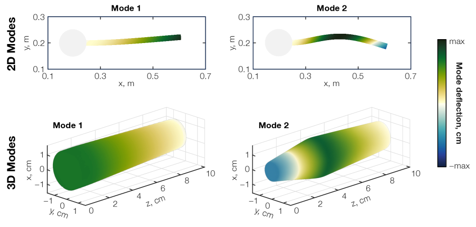
Figure 4: Modal representations of the structure deformation surface: leading modes for the (top) 2D flapping plate and (bottom) 3D flexible pipe.

For the flapping-plate flow, deformation modes are computed via an eigenfrequency analysis of the cylinder–beam assembly using COMSOL. The structure is modeled as a linear, isotropic, elastic solid, with the beam clamped to the rear of a rigid cylinder. The free-vibration problem,

$$\boldsymbol{M}\frac{\partial^{2}\boldsymbol{p}^{\prime}}{\partial t^{2}}+\boldsymbol{K}\boldsymbol{p}^{\prime}=\boldsymbol{0},$$

is recast as a generalized eigenvalue problem,

$$\left(\boldsymbol{K}-\omega_{j}^{2}\boldsymbol{M}\right)\boldsymbol{\varphi}_{j}=\boldsymbol{0},$$

where $\boldsymbol{M}$ and $\boldsymbol{K}$ are the global mass and stiffness matrices, $\omega_{j}$ is the natural circular frequency of the $j$th mode, and $\boldsymbol{\varphi}_{j}$ is the associated spatial eigenvector. Although these modes are not guaranteed to align with the most energetic structural deformations in the FSI response (as POD modes would), they provide a physically meaningful and computationally efficient basis. In our experiments, we retain the first eight modes. The leading two capture approximately 99.85% of the total deformation energy (corresponding to the variance of $\boldsymbol{p}^{\prime}$, while all eight capture 99.98%. The top row of Fig. 4 shows the first two bending modes.

In the 3D flexi-pipe case, we model the surface response using a data-driven POD basis, which directly aligns with the continuous formulation in Sec. 2.3. Deformation snapshots from the simulation are assembled into a matrix of surface displacements, $\boldsymbol{P}^{\prime}=[\boldsymbol{p}^{\prime}(t_{0}),\boldsymbol{p}^{\prime}(t_{1}),\dots]$, and we apply a singular value decomposition,

$$\boldsymbol{P}^{\prime}=\boldsymbol{\Phi}\boldsymbol{\Sigma}\boldsymbol{\Psi}^{\top}.$$

In this expression, $\boldsymbol{\Phi}$ contains spatial deformation modes ordered by energy. POD bases are particularly well suited to empirical workflows, e.g., those involving DIC, since they can be constructed from sparse or asynchronous measurements of the structure. In our experiments, we retain between 1 and 14 modes, accounting for 44.5% and 99% of the total deformation energy, respectively. The first two of these modes are shown in the bottom row of Fig. 4. As in the 2D case, this representation enables us to systematically assess the effect of basis truncation on the accuracy and stability of reconstructions.

5.2 2D Flapping-Plate Flow Reconstructions

We begin by evaluating our framework on the 2D flapping-plate benchmark. Structure deformations are represented using up to eight bending modes for the cylinder–beam assembly, as described above. Sparse particle tracks are generated as outlined in Sec. 4.2. Per Fig. 3, the particle seeding density is especially low near the surface of the plate; moreover, steep velocity gradients and boundary-layer effects in this region reduce the accuracy of particle advection. This produces spatially varying “noise” that is most pronounced near the structure and cannot be corrected using naïve interpolation or smoothing. Consequently, the surface motion must be inferred from off-body data through joint enforcement of the flow physics and the moving-wall boundary condition.

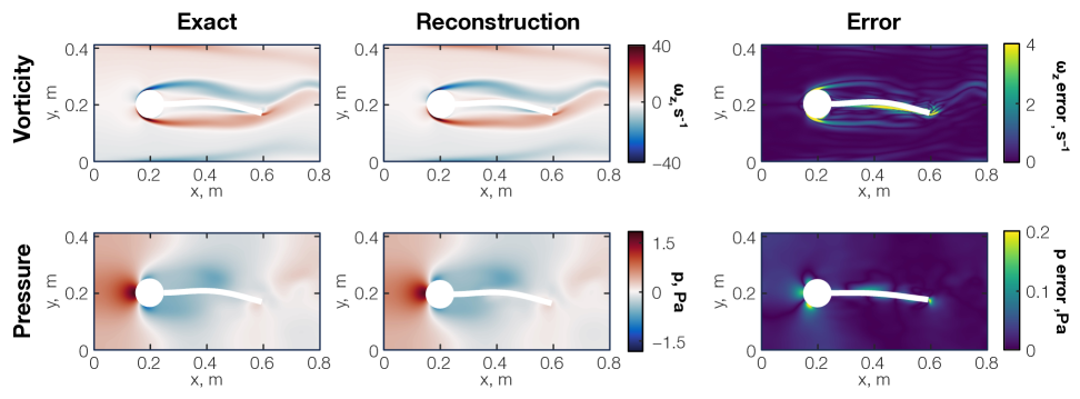
Figure 5: Snapshot of exact (left), reconstructed (middle), and error (right) fields for vorticity (top) and pressure (bottom) in the flapping-plate case. Reconstructions capture key wake dynamics despite sparse, off-body data.

Despite these challenges, our method reconstructs both the fluid and structural states with high fidelity. Figure 5 shows a representative snapshot of the ground truth and reconstructed vorticity and pressure fields. For consistency, both fields are projected onto a structured mesh using a high-accuracy reference PINN trained directly on the ground truth data. The CFD solver produces results on a moving unstructured mesh that conforms to the plate; the shape of the reconstructed plate, by contrast, may differ slightly from the truth shape. As a result, the native CFD solution points do not align with the reconstruction grid. The reference PINN provides smooth interpolation onto a common fixed mesh. The reconstruction captures all salient features of the unsteady wake, including vortex shedding and low-pressure regions in the cylinder’s lee. Normalized root-mean-square errors (NRMSEs) for vorticity and pressure are approximately 15% and 8%, respectively. Errors are elevated along the shear layer and near the surface, consistent with regions of sparse data and steeper gradients. Importantly, reconstruction accuracy remains stable across all modal configurations, confirming that flow inference is unaffected by the inclusion of additional modes that permit high-frequency structural oscillations in regions with sparse particle tracks (or none at all).

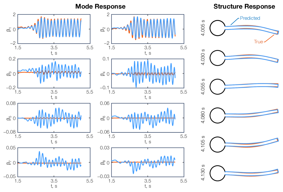
Figure 6: (left) Exact (red) and inferred (blue) mode coefficients for the flapping plate; (right) reconstructed surface shapes at six time instants. Deformations are accurately recovered using the learned coefficients.

Figure 6 shows the time-varying mode coefficients determined by the structure network for the eight-mode case. The leading two modes, which together account for more than 99.85% of the deformation energy, are reconstructed with high accuracy in both amplitude and phase. Higher-order modes exhibit larger deviations, as expected due to their limited energetic contribution and weak observability from off-body data. Still, reconstructed surface shapes closely match the ground truth across the full motion cycle. These results demonstrate the framework’s ability to reconstruct structural motion accurately despite limited and noisy measurements near the fluid–solid interface.

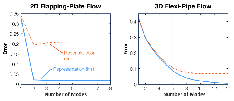
Figure 7: Representation and reconstruction errors vs. modal truncation for the 2D (left) and 3D (right) cases. Errors plateau after capturing the dominant deformation energy (approximately marked by the vertical dashed line), confirming robustness to over-parameterization.

The sensitivity of reconstruction accuracy to modal truncation is analyzed in the left panel of Fig. 7. Each data point corresponds to an independent reconstruction in which the structure model is configured with exactly the modes indicated on the $x$-axis. We compare the representation error,

$$\frac{1}{n_{\mathrm{t}}}\sum_{j=1}^{n_{\mathrm{t}}}\frac{\left\lVert\left(\boldsymbol{I}-\boldsymbol{\Phi}\boldsymbol{\Phi}^{\top}\right)\boldsymbol{p}^{\prime}(t_{j})\right\rVert_{2}^{2}}{\left\lVert\boldsymbol{p}^{\prime}(t_{j})\right\rVert_{2}^{2}},$$

which indicates how well the true deformation is captured by a truncated modal basis, against the actual reconstruction error of the inferred displacements. For the 2D flapping-plate flow case, the representation error drops below 2% after two modes, confirming that the flapping dynamics are effectively low-dimensional. Correspondingly, reconstruction error falls sharply when the second mode is added, from approximately 30% to 20%, and remains relatively flat thereafter. In other words, including more modes beyond this point does not harm performance. This robustness to over-parameterization is a key strength of our approach, particularly for experimental use cases, where the required number of modes may not be known a priori and conservative over-specification may be necessary.

5.3 3D Flexi-Pipe Flow Reconstructions

We next test the framework on a more challenging 3D scenario: pulsatile flow through a compliant straight-walled vessel. As described in Sec. 5.1, structural deformations are modeled using a POD basis extracted from the ground truth simulation. This data-driven basis captures the principal deformation patterns, including wave propagation part-way along the vessel wall, using a compact set of modes. As in the 2D case, particle tracks are sparsely distributed throughout the domain and particularly scarce near the deforming surface, where steep gradients and time-step limitations introduce sampling errors.

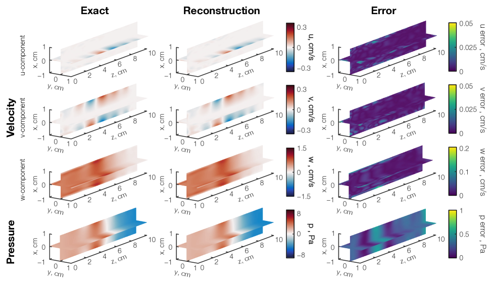
Figure 8: Representative slice of exact (left), reconstructed (middle), and error (right) fields for velocity (top three rows) and pressure (bottom) in the flexi-pipe case. Reconstructions recover axial wave propagation and near-wall vortices.

Figure 8 presents reconstructed flow fields at a representative snapshot. The results accurately capture key features of the ground truth, including transverse vortical structures near the vessel wall and the axial propagation of a pressure-driven wave along the lumen. Time-averaged NRMSEs are approximately 14% for the transverse velocity components, 5% for axial velocity, and 6% for pressure. The largest discrepancies occur near the wall, where sparse particle coverage and steep velocity gradients introduce noise into the synthetic LPT data. Importantly, flow reconstruction accuracy remains consistent across all modal truncations beyond six modes, at which point the reconstruction error saturates around 9%, confirming robustness to over-parameterization.

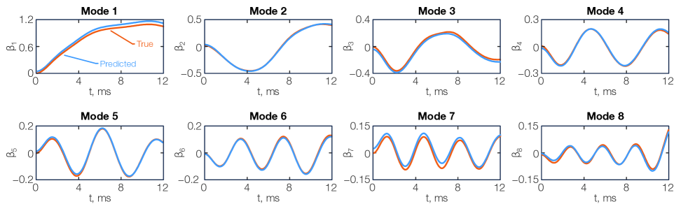
Figure 9: Time series of inferred (blue) and exact (red) POD mode coefficients for the flexible pipe. High accuracy is maintained across all retained modes.

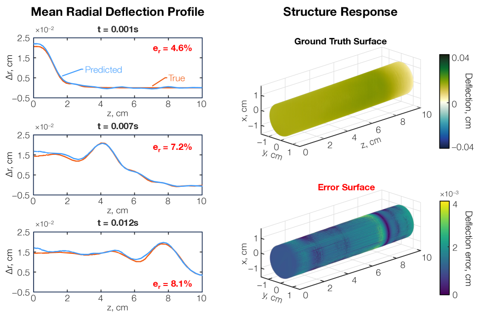
Figure 10: 3D surface shape reconstruction: (left) radial deflection profiles at three time instants and (right) ground truth deformation and corresponding error field at the final frame. The reconstructed bulge tracks the pressure-driven wave observed in the flow.

Figure 9 shows the time series of the inferred POD mode coefficients compared to the ground truth. The predicted modal dynamics closely match the true coefficients across all the retained modes, demonstrating accurate recovery of the dominant structural deformation patterns and the temporal evolution of the propagating wave. Figure 10 illustrates the 3D surface reconstruction results in detail. The left panel shows radial deflection profiles at three representative time instants. Here, the mean radial deflection profile at each $z$ position is computed as the circumferential average of the radial displacement around the pipe cross-section, highlighting the axial propagation of the pressure-driven wave. The predicted profiles match the ground truth well at all times, with relative errors of approximately 4.6%, 7.2%, and 8.1% at the three instants shown. Errors tend to increase slightly over time as the wave propagates and develops sharper gradients, which underscores the difficulties of capturing localized deformations using sparse LPT data. Overall, the reconstruction is reasonably accurate, with relative errors remaining below 9% throughout the entire time interval. The right panel displays the 3D surface deformation at the final time frame, colored by radial deflection magnitude, positioned atop the corresponding error field. The predicted deflection field reproduces the characteristic bulge traveling along the pipe, consistent with the pressure wave propagation revealed in the reconstructed flow fields in Fig. 8.

The right panel of Fig. 7 further illustrates this behavior. Structural reconstruction errors decrease rapidly with the number of retained POD modes, plateauing beyond the eighth mode, which collectively capture over 95% of the deformation energy. As in the 2D case, no instabilities or artifacts are introduced with additional modes, underscoring the framework’s resilience to excess representational capacity. Notably, reconstruction accuracy follows the representation limit of the basis up to six modes, after which performance stabilizes. This insensitivity to basis size is particularly valuable in experimental applications, where the optimal number of modes is unknown. The energy-ordered nature of POD ensures both efficiency and reliability, making this approach attractive for FSI problems where multi-phase empirical measurements can be recorded, such as in vitro hemodynamics simulations or aeroelastic panel flutter.

5.4 Analysis of the Sampling Scheme

All volume and surface loss terms are approximated using Monte Carlo integration. The accuracy of these estimates, and, by extension, the stability of training, depends on the sampling strategy. Variance in the total loss introduced by random sampling propagates to the gradient estimates used during backpropagation. High variance can induce limit-cycle behavior near optima, degrading reconstruction accuracy, or it can prevent convergence altogether. Stable training thus requires low-variance loss approximators that can be computed at reasonable cost. To assess sampling-induced variance, we evaluate different strategies using a randomly initialized network with fixed weights and biases. This provides a conservative baseline that typically bounds the variance encountered during training. For a grid of spatial and temporal sample sizes, we compute 100 independent evaluations of the flow physics loss, surface boundary loss, and particle physics loss for the 2D flapping-plate flow. The standard deviation of each loss term is normalized by its maximum across all configurations, yielding relative variance fields. These results, shown in Fig. 11, inform our batch size selection and allow us to balance the cost and stability of training.

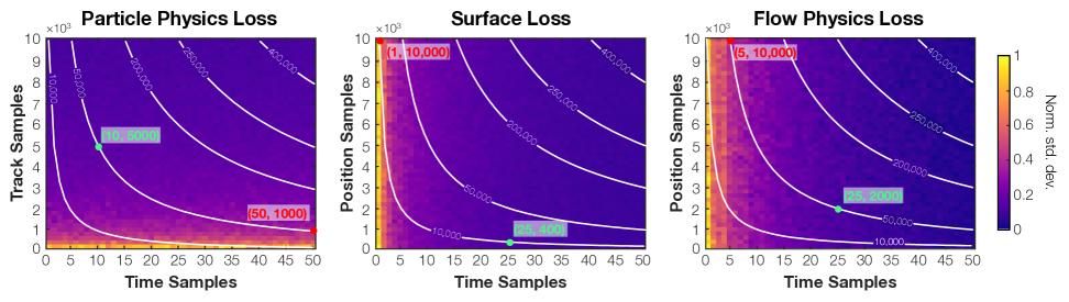
Figure 11: Normalized standard deviation maps for (left to right) particle, boundary, and flow physics loss terms in the the 2D flapping-plate flow case. Axes denote the number of tracks, spatial samples, or temporal samples per iteration. Colors show variance normalized by the maximum for each term. White curves indicate fixed total sample budgets. Green and red dots mark representative favorable and unfavorable sampling strategies.

Trends in Fig. 11 reveal that increasing the number of temporal samples per iteration reduces the variance of the boundary and flow physics loss terms, whereas the number of spatial samples has a weaker effect, likely due to the relatively low spatial complexity of the flow fields and structures in our test cases, e.g., compared to FSI with turbulence, complex shapes, nonlinear structure deformations, etc. The particle physics loss, by contrast, requires sampling tracks, with spatial positions determined by the selected times. In this case, variance is primarily governed by the number of distinct tracks sampled, with a weaker dependence on the number of points sampled per track. In practice, non-ideal seeding or inertial transport effects could further influence the impact of the sampling strategy on variance. Adequate coverage of time and space is essential to ensure representative query points. Figure 11 includes isocontours of the total sample count, which is a proxy for computational cost. When the variance is too high for effective training all the way along the isocontour corresponding to the memory limit of the processing unit(s), gradient averaging across multiple mini-batches can be employed to stabilize optimization (although this was not required in the present study).

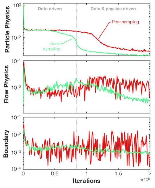
Figure 12: Evolution component-wise loss terms during training for the favorable (green) and poor (red) strategies: (top) particle physics loss, (middle) flow physics loss, (bottom) boundary loss.

To better understand how sampling variance impacts training performance, we reconstructed the 2D flapping-plate flow using two representative sampling strategies: one with low variance (“good sampling”) and one with high variance (“poor sampling”), while keeping the total number of sample points constant. The corresponding configurations are marked by the green (low variance) and red (high variance) dots in Fig. 11. In the good case, we sampled 10 tracks and 5000 time instants for $\mathscr{J}_{\mathrm{part}}$, 400 spatial positions and 25 times for $\mathscr{J}_{\mathrm{surf}}$, and 2000 positions and 25 times for $\mathscr{J}_{\mathrm{flow}}$. In the poor case, we sampled 50 tracks and 1000 times for $\mathscr{J}_{\mathrm{part}}$, 10,000 positions and 1 time for $\mathscr{J}_{\mathrm{surf}}$, and 10,000 positions and 5 times for $\mathscr{J}_{\mathrm{flow}}$.

Evolution of the loss terms over training reveals clear differences between the two sampling strategies. Under the favorable (low-variance) configuration, all loss components decrease smoothly with minimal fluctuations. Training proceeds in three distinct phases. The initial phase, not highlighted in the figure, features a rapid drop in all loss terms by several orders of magnitude. This is followed by a data-driven phase in which the particle loss continues to decrease while the physics losses remain flat or increase slightly, indicating that the network learns to reproduce plausible trajectories without yet satisfying the governing equations. After approximately $8.5\times 10^{4}$ iterations, marked by the vertical gray line in Fig. 12, the flow and boundary losses also begin to decline, signaling the transition to a coupled regime in which data and physics constraints jointly drive the learning. This phase results in more accurate and physically consistent reconstructions of both the flow and the structure. Similar staged behavior was previously reported by Molnar and Grauer [34].

By contrast, the poor (high-variance) sampling strategy, which comes at the same computational cost as the good strategy, results in unstable and inefficient training. All three loss components exhibit high variability, with the flow and boundary losses oscillating erratically throughout training and failing to converge. No clear transition to a coupled regime is observed, and persistently noisy gradient updates appear to impede progress. After roughly $1.2\times 10^{5}$ iterations, the model enters a limit-cycle regime in which short-term reductions in the losses are followed by unpredictable rebounds, preventing sustained improvement. This behavior is quantified using a variance ratio over the final 1000 iterations: under the poor configuration, the flow and boundary loss variances are 7.5-fold and 24-fold higher, respectively, than those under the favorable strategy. These distinct training dynamics translate directly into reconstruction quality. Poor sampling yields final errors of 5.4% in velocity, 17% in pressure, and 50% in the surface reconstruction. The favorable strategy improves all three, reducing the respective errors to 3.5%, 10%, and 20%, underscoring the need to optimize the sampling scheme.

6 Conclusions and Outlook

We present a novel physics-informed framework for reconstructing coupled flow and structural dynamics from sparse single-phase particle tracking data. By integrating fluid and structure PINNs with a moving-wall interface condition, our method infers full-field, time-resolved FSI states from only Lagrangian particle tracks. Notably, it requires no direct structural measurements, no explicit force information, and no constitutive model of the solid; only a precomputed deformation basis and scattered fluid-phase data are needed. This represents a departure from prior FSI reconstruction methods for unsteady flows, which typically require either high-density volumetric data, synchronized multi-phase measurements, or direct structural modeling.

Our method is validated on two canonical benchmark problems. First, we consider vortex-induced vibration of a 2D flexible plate; second, we assess pressure-driven motion in a 3D compliant pipe. In both scenarios, the structural response is accurately inferred entirely from off-body particle tracks, even for sparse data with biased errors in the boundary layers. Reconstruction errors are consistently low across velocity (and velocity gradient), pressure, and deformation fields. Notably, the method is robust to over-parameterization of the structure model: once the dominant deformation modes are included, additional modes do not degrade accuracy, which would indicate ill-posedness. Moreover, accuracy approximately tracks representation error. This removes the need for manual regularization and enhances experimental usability, where the number of active structural modes may be unknown a priori. The approach remains stable and accurate even when structural measurements are unavailable or incomplete, offering a practical pathway to experimental deployment.

From a methodological standpoint, this work introduces a general-purpose, scalable, and physically grounded technique for data assimilation in FSI problems. Its novelty lies in fusing sparse data with differentiable physics solvers to infer both fluid and solid dynamics in a unified inverse framework. This has immediate implications for expanding the use of diagnostic techniques like LPT or MRV (a.k.a. 4D flow MRI), especially in in vitro hemodynamics, aeroelastic testing, and biological flow–structure systems, where structural measurements are often infeasible.

Looking ahead, our priorities are to:

1. systematically characterize reconstruction accuracy under varying measurement densities, noise levels, and temporal resolutions;

2. expand the structure model to accommodate nonlinear materials, large-amplitude deformations, and topological transitions such as contact or buckling; and

3. demonstrate applicability to experimental data, assessing robustness to real-world uncertainties and imperfections.

These developments will further position our framework as a general-purpose, data-efficient tool for inverse reconstruction problems in FSI systems.

References

- [1] T. Nakata and H. Liu, “A fluid–structure interaction model of insect flight with flexible wings,” J. Comput. Phys. 231, 1822–1847 (2012).
- [2] H. Zhu, Q. Sun, X. Liu, J. Liu, H. Sun, W. Wu, P. Tan, and Z. Chen, “Fluid–structure interaction-based aerodynamic modeling for flight dynamics simulation of parafoil system,” Nonlinear Dyn. 104, 3445–3466 (2021).
- [3] A. Calderer, X. Guo, L. Shen, and F. Sotiropoulos, “Fluid–structure interaction simulation of floating structures interacting with complex, large-scale ocean waves and atmospheric turbulence with application to floating offshore wind turbines,” J. Comput. Phys. 355, 144–175 (2018).
- [4] A. Korobenko, M.-C. Hsu, I. Akkerman, J. Tippmann, and Y. Bazilevs, “Structural mechanics modeling and FSI simulation of wind turbines,” Math. Models Methods Appl. Sci. 23, 249–272 (2013).
- [5] H. Suito, K. Takizawa, V. Q. Huynh, D. Sze, and T. Ueda, “FSI analysis of the blood flow and geometrical characteristics in the thoracic aorta,” Comput. Mech. 54, 1035–1045 (2014).
- [6] A. H. Lee, R. L. Campbell, B. A. Craven, and S. A. Hambric, “Fluid–structure interaction simulation of vortex-induced vibration of a flexible hydrofoil,” J. Vib. Acoust. 139, 041001 (2017).
- [7] J. Donea, S. Giuliani, and J.-P. Halleux, “An arbitrary Lagrangian-Eulerian finite element method for transient dynamic fluid-structure interactions,” Comput. Methods Appl. Mech. Eng. 33, 689–723 (1982).
- [8] T. J. Hughes, W. K. Liu, and T. K. Zimmermann, “Lagrangian-Eulerian finite element formulation for incompressible viscous flows,” Comput. Methods Appl. Mech. Eng. 29, 329–349 (1981).
- [9] A. Legay, J. Chessa, and T. Belytschko, “An Eulerian–Lagrangian method for fluid–structure interaction based on level sets,” Comput. Methods Appl. Mech. Eng. 195, 2070–2087 (2006).
- [10] N. Jenkins and K. Maute, “Level set topology optimization of stationary fluid-structure interaction problems,” Struct. Multidiscip. Optim. 52, 179–195 (2015).
- [11] Y. Yu, H. Baek, and G. E. Karniadakis, “Generalized fictitious methods for fluid–structure interactions: analysis and simulations,” J. Comput. Phys. 245, 317–346 (2013).
- [12] A. Pathak and M. Raessi, “A 3D, fully Eulerian, VOF-based solver to study the interaction between two fluids and moving rigid bodies using the fictitious domain method,” J. Comput. Phys. 311, 87–113 (2016).
- [13] C. S. Peskin, “The immersed boundary method,” Acta Numer. 11, 479–517 (2002).
- [14] F. Sotiropoulos and X. Yang, “Immersed boundary methods for simulating fluid–structure interaction,” Prog. Aerosp. Sci. 65, 1–21 (2014).
- [15] G. Hou, J. Wang, and A. Layton, “Numerical methods for fluid-structure interaction—a review,” Commun. Comput. Phys. 12, 337–377 (2012).
- [16] S. Haeri and J. Shrimpton, “On the application of immersed boundary, fictitious domain and body-conformal mesh methods to many particle multiphase flows,” Int. J. Multiphase Flow 40, 38–55 (2012).
- [17] L. Chatellier, S. Jarny, F. Gibouin, and L. David, “A parametric PIV/DIC method for the measurement of free surface flows,” Exp. Fluids 54, 1–15 (2013).
- [18] R. Bleischwitz, R. De Kat, and B. Ganapathisubramani, “On the fluid-structure interaction of flexible membrane wings for MAVs in and out of ground-effect,” J. Fluids Struct. 70, 214–234 (2017).
- [19] P. Zhang, S. D. Peterson, and M. Porfiri, “Combined particle image velocimetry/digital image correlation for load estimation,” Experimental Thermal and Fluid Science 100, 207–221 (2019).
- [20] R. Hortensius, J. C. Dutton, and G. S. Elliott, “Simultaneous planar PIV and sDIC measurements of an axisymmetric jet flowing across a compliant surface,” in “55th AIAA Aerospace Sciences Meeting,” (2017), p. 1886.
- [21] A. D’Aguanno, P. Quesada Allerhand, F. F. J. Schrijer, and B. W. van Oudheusden, “Characterization of shock-induced panel flutter with simultaneous use of DIC and PIV,” Exp. Fluids 64, 15 (2023).
- [22] W. I. Kösters and S. Hoerner, “Simultaneous flow measurement and deformation tracking for passive flow control experiments involving fluid–structure interactions,” J. Fluids Struct. 121, 103956 (2023).
- [23] F. M. Mitrotta, J. Sodja, and A. Sciacchitano, “On the combined flow and structural measurements via robotic volumetric PTV,” Meas. Sci. Technol. 33, 045201 (2022).
- [24] C. J. Elkins and M. T. Alley, “Magnetic resonance velocimetry: applications of magnetic resonance imaging in the measurement of fluid motion,” Exp. Fluids 43, 823–858 (2007).
- [25] A. Kontogiannis, S. V. Elgersma, A. J. Sederman, and M. P. Juniper, “Joint reconstruction and segmentation of noisy velocity images as an inverse Navier–Stokes problem,” J. Fluid Mech. 944, A40 (2022).
- [26] P. Karnakov, S. Litvinov, and P. Koumoutsakos, “Solving inverse problems in physics by optimizing a discrete loss: Fast and accurate learning without neural networks,” PNAS nexus 3, pgae005 (2024).
- [27] A. B. Buhendwa, D. A. Bezgin, P. Karnakov, N. A. Adams, and P. Koumoutsakos, “Shape inference in three-dimensional steady state supersonic flows using ODIL and JAX-Fluids,” arXiv preprint arXiv:2408.10094 (2024).
- [28] M. Raissi, P. Perdikaris, and G. E. Karniadakis, “Physics-informed neural networks: A deep learning framework for solving forward and inverse problems involving nonlinear partial differential equations,” J. Comput. Phys. 378, 686–707 (2019).
- [29] M. Raissi, Z. Wang, M. S. Triantafyllou, and G. E. Karniadakis, “Deep learning of vortex-induced vibrations,” J. Fluid Mech. 861, 119–137 (2019).
- [30] E. Kharazmi, D. Fan, Z. Wang, and M. S. Triantafyllou, “Inferring vortex induced vibrations of flexible cylinders using physics-informed neural networks,” J. Fluids Struct. 107, 103367 (2021).
- [31] H. Tang, Y. Liao, H. Yang, and L. Xie, “A transfer learning-physics informed neural network (TL-PINN) for vortex-induced vibration,” Ocean Eng. 266, 113101 (2022).
- [32] K. Zhou and S. J. Grauer, “Flow reconstruction and particle characterization from inertial Lagrangian tracks,” arXiv preprint arXiv:2311.09076 (2023).
- [33] K. Zhou, R. Tang, G. Ke, and S. J. Grauer, “Neural-implicit particle advection for flow reconstruction from Lagrangian tracks,” in “16th International Symposium on Particle Image Velocimetry (ISPIV 2025),” (2025), p. 24.
- [34] J. P. Molnar and S. J. Grauer, “Flow field tomography with uncertainty quantification using a Bayesian physics-informed neural network,” Meas. Sci. Technol. 33, 065305 (2022).
- [35] S. Wang, Y. Teng, and P. Perdikaris, “Understanding and mitigating gradient flow pathologies in physics-informed neural networks,” SIAM J. Sci. Comput. 43, A3055–A3081 (2021).
- [36] M. Tancik, P. Srinivasan, B. Mildenhall, S. Fridovich-Keil, N. Raghavan, U. Singhal, R. Ramamoorthi, J. Barron, and R. Ng, “Fourier features let networks learn high frequency functions in low dimensional domains,” Adv. Neural Inf. Process. Syst. 33, 7537–7547 (2020).
- [37] J. M. Lee, Smooth Manifolds (Springer, 2003).
- [38] Y. Ma and Y. Fu, Manifold Learning Theory and Applications (CRC Press, 2012).
- [39] J. M. Melenk and I. Babuška, “The partition of unity finite element method: basic theory and applications,” Comput. Methods Appl. Mech. Eng. 139, 289–314 (1996).
- [40] G. Berkooz, P. Holmes, and J. L. Lumley, “The proper orthogonal decomposition in the analysis of turbulent flows,” Annu. Rev. Fluid Mech. 25, 539–575 (1993).
- [41] K. Taira, S. L. Brunton, S. T. Dawson, C. W. Rowley, T. Colonius, B. J. McKeon, O. T. Schmidt, S. Gordeyev, V. Theofilis, and L. S. Ukeiley, “Modal analysis of fluid flows: An overview,” AIAA J. 55, 4013–4041 (2017).
- [42] C. Leake, H. Johnson, and D. Mortari, The Theory of Functional Connections: A Functional Interpolation Framework with Applications (Lulu.com, 2022).
- [43] S. Berrone, C. Canuto, and M. Pintore, “Variational physics informed neural networks: the role of quadratures and test functions,” J. Sci. Comput. 92, 100 (2022).
- [44] Z. Mao and X. Meng, “Physics-informed neural networks with residual/gradient-based adaptive sampling methods for solving partial differential equations with sharp solutions,” Appl. Math. Mech. 44, 1069–1084 (2023).
- [45] X. Wan, T. Zhou, and Y. Zhou, “Adaptive importance sampling for Deep Ritz,” Commun. Appl Math. Comput. pp. 1–25 (2024).
- [46] J. M. Taylor and D. Pardo, “Stochastic Quadrature Rules for Solving PDEs using Neural Networks,” arXiv preprint arXiv:2504.11976 (2025).
- [47] J. P. Molnar and S. J. Grauer, “Algorithm for Time-Resolved Background-Oriented Schlieren Tomography Applied to High-Speed Flows,” in “AIAA SciTech 2025 Forum,” (2025), p. 1060.
- [48] K. Hormann and N. Sukumar, Generalized Barycentric Coordinates in Computer Graphics and Computational Mechanics (CRC Press, 2017).
- [49] S. Turek, J. Hron, M. Madlik, M. Razzaq, H. Wobker, and J. F. Acker, “Numerical simulation and benchmarking of a monolithic multigrid solver for fluid-structure interaction problems with application to hemodynamics,” in “Fluid Structure Interaction II: Modelling, Simulation, Optimization,” , H.-J. Bungartz, M. Mehl, and M. Schäfer, eds. (Springer, 2010), pp. 193–220.
- [50] J. Liu and A. L. Marsden, “A unified continuum and variational multiscale formulation for fluids, solids, and fluid–structure interaction,” Comput. Methods Appl. Mech. Eng. 337, 549–597 (2018).
- [51] A. Updegrove, N. M. Wilson, J. Merkow, H. Lan, A. L. Marsden, and S. C. Shadden, “SimVascular: an open source pipeline for cardiovascular simulation,” Abbreviation Title Ann. Biomed. Eng. 45, 525–541 (2017).
- [52] D. Schanz, S. Gesemann, and A. Schröder, “Shake-The-Box: Lagrangian particle tracking at high particle image densities,” Exp. Fluids 57, 1–27 (2016).